NCIDiff: Non-covalent Interaction-generative Diffusion Model for
Improving Reliability of 3D Molecule Generation Inside Protein Pocket

Abstract

Advancements in deep generative modeling have changed the paradigm of drug discovery. Among such approaches, target-aware methods that exploit 3D structures of protein pockets were spotlighted for generating ligand molecules with their plausible binding modes. While docking scores superficially assess the quality of generated ligands, closer inspection of the binding structures reveals the inconsistency in local interactions between a pocket and generated ligands. Here, we address the issue by explicitly generating non-covalent interactions (NCIs), which are universal patterns throughout protein-ligand complexes. Our proposed model, NCIDiff, simultaneously denoises NCI types of protein-ligand edges along with a 3D graph of a ligand molecule during the sampling. With the NCI-generating strategy, our model generates ligands with more reliable NCIs, especially outperforming the baseline diffusion-based models. We further adopted inpainting techniques on NCIs to further improve the quality of the generated molecules. Finally, we showcase the applicability of NCIDiff on drug design tasks for real-world settings with specialized objectives by guiding the generation process with desired NCI patterns.

1 Introduction

Deep learning models have made impressive progress in various domains, including vision (Ramesh et al., 2021), language (Achiam et al., 2023), and biological science (Jumper et al., 2021; Abramson et al., 2024), particularly with the rise of powerful generative modeling techniques. These generative models enable the sampling of data points based on the learned data distribution from the training set. However, in practice, creating large databases for training often poses challenges due to the time and resources required. In such cases, the real-world settings that these models encounter during inference are likely to be unseen during training, resulting in insecure model performance (van den Burg & Williams, 2021). Drug discovery is one such domain where data is limited, and the value of developing a drug for a novel target — known as a first-in-class drug — is paramount. Therefore, it is necessary to develop reliable and robust molecular generative models that can adapt to novel targets.

Recent advances in deep generative models have enabled the exploitation of structural information from target proteins to generate molecules potentially binding to these targets. This strategy, known as structure-based drug design (SBDD), is particularly advantageous for sampling molecules that can fit into the shape of binding pockets, thereby increasing the likelihood of binding. Various generative model architectures, such as Generative Adversarial Networks (GANs) (Ragoza et al., 2022), auto-regressive models (Luo et al., 2021; Peng et al., 2022; Liu et al., 2022), and diffusion models (Schneuing et al., 2022; Guan et al., 2023; Lin et al., 2022; Guan et al., 2024), have been adopted to carry out SBDD. These models have demonstrated the performance in terms of estimated binding affinity scores, measured by docking programs such as AutoDock Vina (Trott & Olson, 2010).

Despite the impressive ability of these models to generate protein pocket-aware compounds, a closer examination of the generated binding conformers often reveals that they are quite inconsistent with nature. PoseCheck (Harris et al., 2023) highlighted the potential issues that deep SBDD models may confront, especially implausible interactions between a binding pocket and the generated molecules that aggravate the binding stability. Addressing the concern is crucial not only for achieving strong binding but also for fostering dynamically stable binding (Zhung et al., 2024) and providing valuable insights for the hit-to-lead process.

In particular, non-covalent interactions (NCIs) are predominant features in protein-ligand binding (de Freitas & Schapira, 2017). Conventionally, SBDD had leveraged NCIs as additional information to design drug candidates that can gain specificity toward a target or modulate protein activity through precise interactions (Anderson, 2003; Verma et al., 2010; Zhou et al., 2012). These interactions, which include hydrogen bonds, salt bridges, hydrophobic interactions, $\pi$-$\pi$ stacking, and others, occur locally between protein residues and ligand motifs in any given protein-ligand pair. The universality of NCIs across protein-ligand interfaces suggests that they can serve as key features in generalizing deep learning models. Previous deep learning-based approaches (Moon et al., 2022, 2024; Méndez-Lucio et al., 2021; Shen et al., 2022; Seo & Kim, 2023) with objectives including protein-ligand binding affinity prediction, binding pose prediction, and virtual screening have shown that utilizing NCIs can improve the robustness of model performance over unseen data while highlighting model reliability by providing interpretation related to NCIs.

However, existing generative models often overlook NCIs despite their significance, while only a few have taken them into consideration. DeepICL (Zhung et al., 2024) and InterDiff (Wu et al., 2024) explicitly employ an NCI pattern as a condition of protein atoms to induce a molecule generation with desired NCIs. Nevertheless, while NCI patterns are closely aligned with the ligand generative process, one cannot validate the given NCI condition before the sampling process unless the presence of ligand binding information of a target pocket. Lingo3DMol (Feng et al., 2024) uses a separate model to predict NCI patterns to address this issue; however, the ligands sampled from the model may be biased toward the deterministic predictor, limiting the robustness for novel targets. Since NCI patterns are intimately correlated with how and which a ligand binds to a pocket, simultaneously learning suitable NCI patterns between a protein and a ligand, along with the ligand structure itself, is needed for a model to featurize generalizable patterns of protein-ligand binding. Such a strategy is essential to address the growing demand for a reliable generative model in SBDD, yet none of the previous works has attempted it.

In this light, we propose NCIDiff, an NCI-generative diffusion model that autonomously generates NCI patterns while generating a molecule inside a given protein pocket. Since a protein-ligand complex can serve as a large bipartite graph, we formulate the ligand design task into modeling the full graph from a given protein graph. More specifically, our model generates a 3D graph of a ligand that comprises covalent intra-edge types, node types, and positions, and at the same time, non-covalent inter-edge types between a protein and a ligand. We devise multiple techniques to deal with the sparse NCIs, effectively considering the local environment that can align with the objective of diffusion-based generation. Moreover, coupling with the inpainting method, we provide an NCI-guided generation scheme for generating molecules with the desired NCI patterns.

To substantiate the reliability of our model, we carefully assess the ligands generated by NCIDiff in various aspects. While previous diffusion-based models often fall short when considering the locality of the protein-ligand interface, the generated ligands from NCIDiff form a larger number of NCIs on top of higher docking scores. Additionally, we demonstrate the enhancement in the model performance by guiding the generation process with the retrieved NCI patterns from the pre-sampled ligands, rationalizing the designed NCI patterns from our model. Furthermore, we emphasize the applicability of an NCI-guided design scheme to target-specific tasks where previous diffusion-based SBDD models have not been challenged despite its importance in rational drug design.

Our contributions are summarized as follows:

• We propose NCIDiff, a diffusion-based generative model that concurrently generates a full 3D graph of a ligand with corresponding NCIs inside a target protein pocket.

• We devise multiple techniques to properly generate NCI patterns during the generative process, tackling the sparse nature of NCIs.

• We evaluate the generated ligands in terms of NCIs, demonstrating that exploiting NCIs can improve the reliability of the deep SBDD model.

• We highlight the applicability of NCIDiff in real-world settings by utilizing an NCI-guided ligand design scheme, gaining crucial properties in drug design, such as selectivity.

2 NCIDiff: NCI-generative Diffusion Model

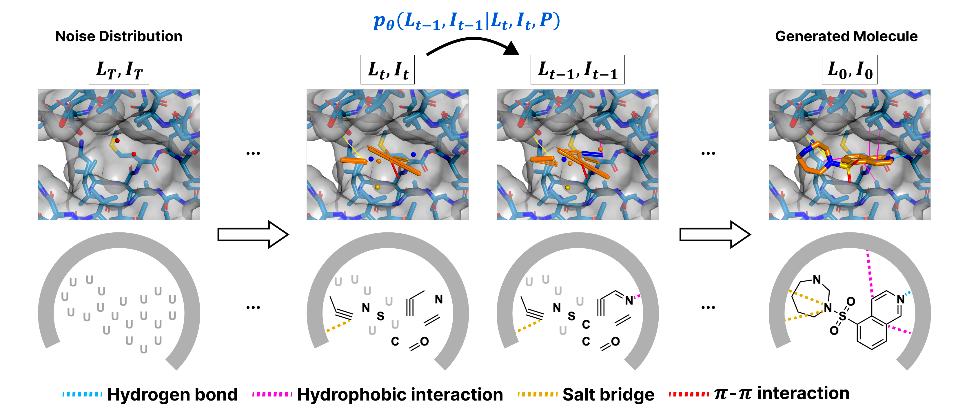
Figure 1: The illustration of a generation process of NCIDiff, where the 3D graph of a ligand and NCIs are denoised concurrently.

We propose the Non-Covalent Interaction-generative denoising Diffusion probabilistic model (NCIDiff) for generating molecules inside a protein pocket. Our model constructs 3D molecular graphs along with NCI types between ligand and protein atoms from a given protein structure. Specifically, a protein pocket is provided as $P=\{(h_{i}^{\textnormal{P}},x_{i}^{\textnormal{P}},e_{ij}^{\textnormal{P}})\}_{i,j\in\{1,2,...,N_{P}\}}$ where $N_{P}$ denotes the number of protein atoms. $h_{i}^{\textnormal{P}}$ and $e_{ij}^{\textnormal{P}}$ denotes a protein node and edge feature, respectively, and $x_{i}^{\textnormal{P}}\in\mathbb{R}^{3}$ denotes a position of a protein atom. The generated output, comprising molecule and NCIs, is provided as $L=\{(h_{i}^{\textnormal{L}},x_{i}^{\textnormal{L}},e_{ij}^{\textnormal{L}})\}_{i,j\in\{1,...,N_{L}\}}$ and $I=\{\mathbf{i}_{ij}\}_{i\in\{1,...,N_{P}\},j\in\{1,...,N_{L}\}}$ where $N_{L}$ denotes the number of ligand atoms. $h_{i}^{\textnormal{L}}$ and $e_{ij}^{\textnormal{L}}$ denotes a ligand node and edge feature, respectively, and $x_{i}^{\textnormal{L}}\in\mathbb{R}^{3}$ denotes a position of a ligand atom. $\mathbf{i}_{ij}$ is an NCI type between a protein and ligand atom. For simplicity, we abbreviate the notation of the generated ligand and its NCIs as $[h,x,e,\mathbf{i}]$.

2.1 Forward Diffusion Process for NCIs

Given the significance of the non-covalent interaction features in rational drug design, we incorporated a diffusion process for a full bipartite graph for a protein-ligand complex. We extract the NCI patterns of protein-ligand complexes via protein-ligand interaction profiler (PLIP) (Salentin et al., 2015). Six NCI types are considered: hydrogen bond donors and acceptors, salt bridge cations and anions, hydrophobic interactions, and $\pi$-$\pi$ interaction. Following the progress in diffusion models on continuous space (Ho et al., 2020) and discrete space (Austin et al., 2021), at each timestep $t$, an atom position distribution is shifted towards the standard Gaussian distribution by adding small Gaussian noise. An atom type, bond type, and NCI type distributions are shifted towards a specific distribution. The forward diffusion process for diffusion timestep $t$ is as follows:

$$q(L_{t},I_{t} \mid L_{t-1},I_{t-1},P)=$$ (1)

$$\ q(h_{t}|h_{t-1}) \cdot q(x_{t}|x_{t-1})\cdot\ q(e_{t}|e_{t-1})\cdot q(\mathbf{i}_{t}|\mathbf{i}_{t-1}),$$

while the forward diffusion process of continuous atom position $x_{t}$ and categorical $h_{t}$, $e_{t}$, $\mathbf{i}_{t}$ are denoted as follows:

$$q(x_{t}|x_{t-1})=\mathcal{N}(x_{t};\sqrt{1-\beta_{t}}x_{t-1},\beta_{t}\mathbf{{I}}),$$ (2)

$$q(\mathbf{i}_{t}|\mathbf{i}_{t-1})=\mathcal{C}(\mathbf{i}_{t};\mathbf{i}_{t-1}Q_{t}),$$ (3)

with the predefined noise schedule, $\beta_{1},\cdots,\beta_{T}$, while $h_{t}$ and $e_{t}$ follow the same Equation 3.

The probability transition matrix $Q_{t}$ introduces a small noise shifting towards a certain probability mass, known as the absorbing type, by slightly decreasing the probability of $h_{t-1}$. For bonds and NCIs, the non-bonding and non-NCI types are naturally set as the absorbing types, respectively. For atom types, an additional masking atom type, depicted as $U$ in Figure 1, is introduced as an absorbing type. With the $m$-th index as the absorbing type, the probability transition matrix is as follows:

$$[Q_{t}]_{ij}=\begin{cases}1&\text{if }i=j=m\\ 1-\beta_{t}&\text{if }i=j\neq m\\ \beta_{t}&\text{if }j=m,i\neq m\text{.}\end{cases}$$ (4)

The choice of the noise schedule for each of $[h,x,e,\mathbf{i}]$ varies in the implementation; for convenience, we unified the notation $\beta_{t}$ regardless of the entity type. The protein-ligand complex’s overall distribution is decomposed into node, position, edge, and NCI features, each treated as independent distributions. By the Markov property, $L_{t}$ and $I_{t}$ can be directly obtained as a closed form from the data $L_{0}$ and $I_{0}$ with $\alpha_{t}=1-\beta_{t}$, $\mkern 1.5mu\overline{\mkern-1.5mu\alpha\mkern-1.5mu}\mkern 1.5mu_{t}=\prod_{s=1}^{t}\alpha_{s}$, and $\mkern 1.5mu\overline{\mkern-1.5muQ\mkern-1.5mu}\mkern 1.5mu_{t}=Q_{1}Q_{2}\ldots Q_{t}$ as follows:

$$q(x_{t}|x_{0}) =\mathcal{N}(x_{t};\sqrt{\mkern 1.5mu\overline{\mkern-1.5mu\alpha\mkern-1.5mu}\mkern 1.5mu_{t}}x_{0},(1-\mkern 1.5mu\overline{\mkern-1.5mu\alpha\mkern-1.5mu}\mkern 1.5mu_{t})\mathbf{{I}}),$$ (5)

$$q(\mathbf{i}_{t}|\mathbf{i}_{0}) =\mathcal{C}(\mathbf{i}_{t};\mathbf{i}_{0}\mkern 1.5mu\overline{\mkern-1.5muQ\mkern-1.5mu}\mkern 1.5mu_{t}),$$ (6)

where $h_{t}$ and $e_{t}$ are the same as Equation 6. For large $t$, The distribution of atom, bond types, and NCI types will be a point mass distribution to the absorbing type, while the distribution of atomic positions will become standard Gaussian distribution.

2.2 Reverse Generative Process

During the reverse generative process, a molecule is generated from the initial noise distribution $\mathcal{N}(\mathbf{0},\mathbf{I})$, centered on the protein pocket centroid for atom positions and point mass categorical distribution on the absorbing type. A single step posterior for atom, bond, and NCI types and atom positions can be obtained by Bayes rule as follows:

$$q(x_{t-1}|x_{t},x_{0}) =\mathcal{N}(x_{t-1};\tilde{\mu}_{t}(x_{t},x_{0}),\tilde{\beta}_{t}\mathbf{I}),$$ (7)

$$q(\mathbf{i}_{t-1}|\mathbf{i}_{t},\mathbf{i}_{0}) =\mathcal{C}\biggl{(}\mathbf{i}_{t-1};\frac{\mathbf{i}_{t}Q_{t}^{\top}\odot\mathbf{i}_{0}\mkern 1.5mu\overline{\mkern-1.5muQ\mkern-1.5mu}\mkern 1.5mu_{t-1}}{\mathbf{i}_{0}\mkern 1.5mu\overline{\mkern-1.5muQ\mkern-1.5mu}\mkern 1.5mu_{t}\mathbf{i}_{t}^{\top}}\biggr{)},$$ (8)

where $\odot$ indicates an element-wise product, $\tilde{\mu}_{t}(x_{t},x_{0}):=\frac{\sqrt{\mkern 1.5mu\overline{\mkern-1.5mu\alpha\mkern-1.5mu}\mkern 1.5mu_{t-1}}\beta_{t}}{1-\mkern 1.5mu\overline{\mkern-1.5mu\alpha\mkern-1.5mu}\mkern 1.5mu_{t}}x_{0}+\frac{\sqrt{\alpha}_{t}(1-\mkern 1.5mu\overline{\mkern-1.5mu\alpha\mkern-1.5mu}\mkern 1.5mu_{t-1})}{1-\mkern 1.5mu\overline{\mkern-1.5mu\alpha\mkern-1.5mu}\mkern 1.5mu_{t}}x_{t}$, and $\tilde{\beta}_{t}:=\frac{1-\mkern 1.5mu\overline{\mkern-1.5mu\alpha\mkern-1.5mu}\mkern 1.5mu_{t-1}}{1-\mkern 1.5mu\overline{\mkern-1.5mu\alpha\mkern-1.5mu}\mkern 1.5mu_{t}}\beta_{t}$. We wrote the equation of posterior in categorical space only for atom types as Equation 8; atom and bond types also follow the same equation.

To match the true reverse generative posterior, we parameterize the reverse process, $p_{\theta}(L_{t-1},I_{t-1}|L_{t},I_{t},P)$. Starting from $L_{0}$ and $I_{0}$, we first sample $L_{t}$ and $I_{t}$ by Equation (5) and (6). The model $\mathcal{X}_{\theta}$ predicts $\hat{L}_{0}$ and $\hat{I}_{0}$, with the training objective defined as follows:

$$\hat{L}_{0},\hat{I}_{0}=\mathcal{X}_{\theta}(L_{t},I_{t},t,P),$$ (9)

Loss $$=D_{\text{KL}}\bigl{(}q(L_{t-1}|L_{t},L_{0})\|p_{\theta}(L_{t-1}|L_{t},\hat{L}_{0})\bigr{)}$$

$$+D_{\text{KL}}\bigl{(}q(I_{t-1}|I_{t},I_{0})\|p_{\theta}(I_{t-1}|I_{t},\hat{I}_{0})\bigr{)}.$$ (10)

Adopting the model architectures for $E(3)$-equivariant inputs, we parameterize the reverse process using $E(3)$-equivariant graph neural networks (GNNs). While (Satorras et al., 2021) was designed to update node features and positions for a homogeneous graph, a protein-ligand complex is a bipartite graph with heterogeneous NCI edges. Additionally, the number of edges for NCI predictions scales up to $N_{P}\times N_{L}$, while the number of actual NCIs is sparse. Therefore, designing an $E(3)$-equivariant GNN architecture that propagates messages through a bipartite graph and reduces its computational burden is necessary. For this purpose, we devise an $E(3)$-equivariant dynamic interaction network that includes sparse edge updates through a full graph of a protein-ligand complex, where detailed architecture is described in Appendix B. Here, while defining the neighboring atoms, we employ radial cutoff, $\gamma_{t}$, to prune the edges with far distances so that the local environment can be more focused. Note that the radial cutoff distance depends on the timestep $t$, where the cutoff value decreases during the generative process. Intuitively, in the early stage of generation, it is important to learn the global structure, while the local structure becomes important in the final steps. We select the simplest linear function for scheduling the radial cutoff as follows:

$$\gamma_{t}=\gamma_{\text{min}}+\frac{t}{T}(\gamma_{\text{max}}-\gamma_{\text{min}}),$$ (11)

where the choice for minimum and maximum cutoff values, $\gamma_{\text{min}}$ and $\gamma_{\text{max}}$, differs between intra (covalent) and inter (non-covalent) edges. Detailed values are provided in Appendix F.

After sparsifying the edges of a bipartite graph of a protein-ligand complex, messages are calculated and propagated through edges to update $h^{\text{P}},h^{\text{L}},e^{\text{P}},e^{\text{L}},x^{\text{L}},$ and $\mathbf{i}$ through Equation (16) to (21). Note that the position update is only applied to ligand atoms. After updating features and positions through $l$ layers of dynamic interaction networks, the final atom types, bond types, and NCI types are sampled from passing through multi-layer perceptions (MLPs) followed by softmax activation.

2.3 Diffusion Strategies for Modeling NCIs

Separate noise schedule The forward noising schedule $\beta_{1:T}$ of NCIDiff is defined independently for each entity. In the case of molecule generation, atom positions, bonds, and NCIs have a strong dependency. Previous studies (Peng et al., 2023; Vignac et al., 2023) have suggested that defining a bond-first noise schedule can enhance the quality of generated molecules by following a more realistic noising process. We extend this concept to the NCI noising schedule. Intuitively, while NCIs still strongly depend on the distance between atoms, their distribution is less peaked compared to bond lengths. Consequently, a noise schedule in the order of bond $\rightarrow$ NCI $\rightarrow$ atom is applied during the forward process. Specific hyperparameters for separate noise scheduling are provided in Appendix D.

Local geometry guidance Bond distances, bond angles, and NCI distances usually fall in certain ranges. Several studies (Peng et al., 2023; Guan et al., 2024; Qian et al., 2024) have shown that the incorporation of prior knowledge on bond distance during the sampling process greatly enhances the generated molecule samples. We extend this concept to the bond angles and NCIs. The bond distance, bond angle, and NCI distance guidance terms are computed at each timestep during the reverse generative process, adding drift terms to sample $x_{t-1}$ as follows:

$$\mu_{\theta}^{\prime}(x_{t},t) =\mu_{\theta}(x_{t},t)+\delta_{\text{BD}}+\delta_{\text{ID}}+\delta_{\text{BA}},$$ (12)

$$x_{t-1} \sim\mathcal{N}(x_{t-1};\mu_{\theta}^{\prime}(x_{t},t),\tilde{\beta}_{t}\mathbf{I}),$$

where $\mu_{\theta}(x_{t},t)$ is a model-predicted $\tilde{\mu}_{t}(x_{t},x_{0})$, while $\delta_{\text{BD}}$, $\delta_{\text{ID}}$, and $\delta_{\text{BA}}$ denotes the guidance terms for bond distance, bond angle, and NCI distance, respectively. Appendix F includes details for each local geometry guidance term.

Method	Vina Dock ($\downarrow$)		QED ($\uparrow$)		SA ($\uparrow$)		Diversity	# NCI edge ($\uparrow$)
	Avg.	Median	Avg.	Median	Avg.	Median		SB	HB	HI	PP
AR	-6.85	-6.66	0.51	0.51	0.64	0.63	0.84	2.56	3.21	3.24	4.82
GraphBP	-6.41	-6.12	0.45	0.48	0.49	0.49	0.79	0.44	1.31	5.75	0.06
Pocket2Mol	-7.03	-6.76	0.58	0.59	0.75	0.76	0.85	1.57	0.96	3.70	14.2
TargetDiff	-7.56	-7.50	0.48	0.49	0.61	0.59	0.78	2.44	4.17	4.40	5.61
InterDiff*	-7.08	-7.00	0.32	0.28	0.56	0.56	0.81	3.01	4.77	4.33	1.98
NCIDiff	-7.29	-7.31	0.47	0.48	0.64	0.65	0.81	5.57	3.93	4.16	6.57
NCIDiffref*	-7.52	-7.48	0.48	0.48	0.67	0.67	0.79	6.75	3.95	4.06	7.95
NCIDiffopt	-7.70	-7.75	0.42	0.43	0.65	0.66	0.80	7.78	4.76	5.66	11.33
Reference	-7.52	-7.48	0.48	0.47	0.73	0.74	-	4.81	4.01	3.51	9.32

Table 1: Evaluation of baseline models along with NCIDiff. SB: salt bridge, HB: hydrogen bond, HI: hydrophobic interaction, and PP: $\pi$-$\pi$ stacking. The asterisk indicates methods that require reference NCI patterns from the test set. We highlight the best results with bold text and the second best with underlined text, respectively.

2.4 NCI-guided Molecule Generation

In classical molecule design tasks, molecules are often designed by anchoring or avoiding certain NCIs (Bhujbal et al., 2022). Previous methods access these concepts by conditional generation (Zhung et al., 2024; Feng et al., 2024; Wu et al., 2024), with NCIDiff considering NCIs as a generative posterior, we use the inpainting method to fix the type of NCI edges during the generation. While (Schneuing et al., 2022) directly inpaints the atom positions for ligand elaboration purposes, our approach can generate molecules with diverse structures that share the desired NCI pattern. Leveraging recent advances in inpainting diffusion models that utilize resampling (Anciukevičius et al., 2023; Lugmayr et al., 2022), we propose an NCI-guided molecule generation approach.

Specifically, for desired NCI types within a protein pocket, $I^{\text{fix}}=\{{\color[rgb]{0,0,0}\mathbf{i}_{ij}}\}_{i\in\{1,...,N_{P}\},j\in\{1,...,N_{L}\}}$, a binary interaction mask, $m^{\text{fix}}=\{{\color[rgb]{0,0,0}m_{ij}}\}_{i\in\{1,...,N_{P}\},j\in\{1,...,N_{L}\}}$ can be defined. An entry of an interaction mask, ${\color[rgb]{0,0,0}m_{ij}}\in\{0,1\}$, denotes 1 if the NCI type between a protein and ligand atom is desired to be fixed. Utilizing this mask matrix, a single-step sampling with inpainting is performed as follows:

$$I^{\text{fix}}_{t-1} \sim q(I^{\text{fix}}_{t-1}|I_{t},I^{\text{fix}}_{0}),$$ (13)

$$I_{t-1}^{\text{gen}} \sim q(I_{t-1}^{\text{gen}}|I_{t},\hat{I}_{0}),$$ (14)

$$I_{t-1} =m^{\text{fix}}\odot I^{\text{fix}}_{t-1}+(1-m^{\text{fix}})\odot I_{t-1}^{\text{gen}}.$$ (15)

However, it is known that inpainting diffusion models can result in samples overlooking global information. Since the SBDD task involves both local (bond and NCIs) and global (QED and SA) objectives, we leverage the RePaint technique inspired by the previous work (Lugmayr et al., 2022). The RePaint process involves iterative resampling steps that allow the model to make more substantial changes than a single-step reverse sampling would permit, resulting in more harmonized samples. The specific algorithm of the RePaint mechanism is provided in Algorithm 1.

Inspired by classical methods exploiting 3D ligand information for identifying key residues and interactions (Bhujbal et al., 2022), we devise a generative pipeline that retrieves plausible NCIs identified from pre-sampled ligands. From ligands generated without any fixed NCIs, every generated NCI pattern is merged to obtain a probability of a specific pocket atom having a specific NCI type. An NCI pattern, $I^{\text{opt}}$, is then sampled from the NCI probability density, $p(I|P)$. A detailed algorithm of sampling $I^{\text{opt}}$ is described in Algorithm 2. We pre-sampled 100 ligands per test pocket for the first round. In the second round generation, $I^{\text{opt}}$ is sampled and fixed for inpainting while again generating 100 ligands for each test pocket. We named this method as NCIDiff^opt.

2.5 Sampling the Number of Ligand Atoms

In SBDD, the sizes of molecules significantly influence their affinities toward a target protein. However, this topic has not been thoroughly explored in deep learning-based SBDD. Auto-regressive models (Luo et al., 2021; Zhung et al., 2024) were able to learn the distribution of the number of atoms by training the model to predict a stop token. However, geometric diffusion models require a given prior distribution $p(N_{L}|{P})$ to generate a 3D molecule in the pocket. (Guan et al., 2023; Wu et al., 2024) utilized a distribution of the distance of the farthest atom pair in a target pocket to estimate the number of ligand molecules, but this approach heavily depends on a reference ligand. For more robust and ligand-free atom number sampling, we utilized POcket Volume MEasurer 2 (POVME2) (Durrant et al., 2014) to measure pocket volumes. Then, we construct a prior distribution of measured pocket volume and the number of ligand atoms in the training set, which is an estimation of $p(N_{L}|p)$. More details about POVME2 parameters and fitting methods are presented in Appendix C.

3 Experiments

3.1 Experimental Setup

Dataset We used CrossDocked2020 dataset (Francoeur et al., 2020) to train and test NCIDiff. Following the previous works, we curated the initial set of 22.5 million docked protein-ligand complexes by choosing only those with binding pose RMSD of less than 1 $\mathrm{\text{\AA}}$ (Luo et al., 2021; Guan et al., 2023). Then, the sequence split of the train and test set was done with sequence identity below 30 %. This process resulted in a final dataset of 100,000 complexes for training and 100 complexes for test.

Baselines We benchmark our model compared to other deep SBDD models, which generate a 3D ligand inside the protein pocket. AR (Luo et al., 2021) is a point cloud-based auto-regressive generative model that generates molecules by placing atoms sequentially in a protein pocket. GraphBP (Liu et al., 2022) and Pocket2Mol (Peng et al., 2022) are also auto-regressive methods but generate molecules as 3D graphs. TargetDiff (Guan et al., 2023) is a state-of-the-art point cloud-based diffusion model. InterDiff (Wu et al., 2024) is also a point cloud-based diffusion model but generates molecules with a given NCI prompt as a condition on protein atoms.

Evaluation We focused on assessing a generated molecule in target binding affinity, molecular properties, and the number of NCI edges for each type measured from the generated pose. For molecular properties, we evaluate the quantitative estimate of drug-likeness (QED) (Bickerton et al., 2012), synthetic accessibility (SA) (Ertl & Schuffenhauer, 2009), and diversity. NCIDiff, as an SBDD model with a full generation of inter and intra-edge features, excluding post-processing such as OpenBabel software (O’Boyle et al., 2011), focuses more on the reliability and interactions of the generated molecules. We used Vina (Trott & Olson, 2010) to evaluate the affinity of the generated molecules and PLIP (Salentin et al., 2015) to evaluate the number of NCI edges of the generated molecules.

3.2 Main Results of NCIDiff

First, we assessed the binding affinities of generated molecules in terms of the Vina docking score. We also evaluated the generated molecules’ binding mode in terms of NCIs, which play a major part in the stability of molecule binding to a target protein. Additionally, we compared NCIDiff^opt, which retrieves the generated interactions from the pre-sampling while still being a reference ligand-free method. As shown in Table 1, NCIDiff outperformed AR, GraphBP, and Pocket2Mol in most of the structure-related metrics.

Particularly in NCI metrics, where other baseline models struggled to create salt bridges (AR: 2.56), NCIDiff generated salt bridges exceeding those observed in the reference ligands in the test set. For other NCIs, TargetDiff showed competitive results with a higher number of hydrogen bonds and hydrophobic interactions but lower in salt bridges and $\pi$-$\pi$ stacking, while other models generated an insufficient number of interactions (AR) or showed barely any interactions in some categories (GraphBP: $\pi$-$\pi$ stacking, Pocket2Mol: hydrogen bonds). Notably, NCIDiff^opt showed significant improvement over NCIDiff by generating a substantial number of NCIs for all types while either outperformed or comparable among the baselines. Additionally, NCIDiff^opt achieved the lowest Vina docking score among the baseline methods.

Meanwhile, NCIDiff lagged behind the best-performing auto-regressive model, Pocket2Mol, in molecular property benchmarks, including QED and SA. However, our results achieved higher QED and SA scores compared to TargetDiff and InterDiff, accounting for its explicit consideration of a molecular graph during the diffusion generative process.

Lastly, we report the results for NCIDiff^ref, which inpaints reference NCI patterns extracted from the protein-ligand complexes of the test set. Compared to InterDiff, NCIDiff outperformed in most metrics, including structure- and property-related ones. Specifically, NCIDiff^ref generates molecules with a lower Vina docking score of -7.50 kcal/mol, which is lower than -7.08 kcal/mol of InterDiff that uses the same reference ligands for extracting NCI patterns. For interaction metrics, InterDiff slightly outperformed in generating hydrogen bonds and hydrophobic interactions, while NCIDiff^ref generated significantly more salt bridges and $\pi$-$\pi$ stackings. Notably, even in the NCI benchmarks where NCIDiff falls behind, NCIDiff^ref still generated NCIs similar numbers to the reference ligands.

3.3 Ablation Studies

Effect of considering NCIs The key features of NCIDiff are treating NCIs as a generative posterior and incorporating guidance during generation. We conducted ablation studies on these features to validate the efficacy of our strategies. First, we generated molecules using the same settings as NCIDiff but removed the interaction distance guidance term (w/o guidance). Second, we trained a separate model (w/o NCI), an SBDD model with the same settings as NCIDiff but without the NCI-related features, thus a mere 3D graph generative model in protein pocket. Table 2 shows the effect of using interaction distance guidance that all metrics were lower when removing the guidance term. Moreover, the comparison between the w/o guidance and the w/o NCI model provides a strict ablation of using NCIs as a generative posterior. Since the w/o guidance model outperformed most of the metrics (SB, HB, and HI) on the w/o NCI model, it suggests that considering NCIs during training and generation remains beneficial.

	# NCI edge ($\uparrow$)
	SB	HB	HI	PP
NCIDiff	5.57	3.93	4.16	6.57
w/o guidance	4.64	3.81	4.00	5.21
w/o NCI	3.45	3.71	3.57	7.21

Table 2: The effect of considering NCIs in terms of distance guidance or generative posterior.

Effect of RePaint To demonstrate the effectiveness of the resampling process described in 2.4, we assess NCIDiff^ref-generated ligands without using the RePaint technique (w/o RePaint). As shown in Table 3, the RePaint technique improved the performance in a structure-related metric (Vina scores) and topology-related metrics (QED and SA), implying an improvement in considering the global context.

	Vina Dock ($\downarrow$)		QED ($\uparrow$)		SA ($\uparrow$)
	Avg.	Median	Avg.	Median	Avg.	Median
NCIDiffref	-7.52	-7.48	0.48	0.48	0.67	0.67
w/o RePaint	-7.28	-7.29	0.47	0.47	0.65	0.65

Table 3: The effect of RePaint ablated on NCIDiff^ref.

3.4 Demonstrating the Reliability of NCIDiff

To further demonstrate the reliability of NCIDiff, we explored the impact of NCIs in anchoring the binding pose. The RMSD of a ligand after redocking is often used as a metric to evaluate the stability of its binding pose. Moreover, if the interactions from the binding pose are relevant, the stability would increase with a higher number of interactions. Thus, we analyzed the tendency of docking RMSDs with respect to the number of hydrogen bonds within the generated ligands.

Figure 2 shows the result of our inspection. Interestingly, we found out that the docking RMSDs of the generated ligands from NCIDiff constantly decrease as we leave the ligands that form more hydrogen bonds with the pockets. In contrast, the generated ligands from TargetDiff exhibit the opposite tendencies. Although the docking RMSD value of NCIDiff was larger when the ligands with fewer hydrogen bonds were included, it flipped when the generated ligands could form more than 6 hydrogen bonds. The docking RMSD value has been decreased by 3.56 $\mathrm{\text{\AA}}$ when the generated ligands include more than 10 hydrogen bonds, showing a significant gap with TargetDiff.

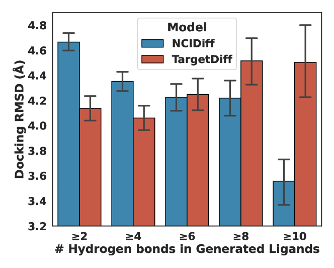
Figure 2: The bar plot shows docking RMSDs of generated ligands from NCIDiff and TargetDiff, with the number of hydrogen bonds over the threshold values. Error bars indicate 95% confidence intervals.

3.5 Applications of NCI-guided Ligand Design

Mutant-selective EGFR inhibitor design We aimed to design potent mutant-selective inhibitors for epidermal growth factor receptor (EGFR), a challenging task in medicinal chemistry to reduce the adverse effects by sparing the wild-type (WT) receptor. From (Sogabe et al., 2013), we retrieved two EGFR complex structures (PDB ID: 3w2s and 3w2r) that share the same ligand. Both pockets have very similar structures, except two residues — Met790 and Arg858 — are mutated in one pocket. To gain selectivity toward the mutant pocket, we hypothesized that forming NCIs with the mutated residues would be beneficial. Thus, we set the NCI pattern that interacts with the side chains of the two residues and utilized it for inpainting. After generating 200 valid ligands inside the mutant pocket, we docked them in both WT and mutant pockets to obtain Vina scores.

Figure 3 illustrates the result, where the points above the black diagonal line score lower on the mutant pocket. The black star corresponds to a reference ligand from the original complexes. As a baseline, we employed TargetDiff to follow the same experimental scheme. The generated ligands from TargetDiff show almost the same Vina score distribution regardless of the mutation, reporting mean values of -9.11 and -9.22 kcal/mol for mutant and WT EGFR, respectively. This indicates that a ligand design with a mere pocket structure cannot induce selectivity. In contrast, our strategy successfully motivates our model to gain asymmetric distribution where mean values are -11.23 and -10.12 kcal/mol, respectively. Notably, the scores on the mutant pocket are lower than those on the WT pocket, suggesting the potential selectivity toward the mutant EGFR.

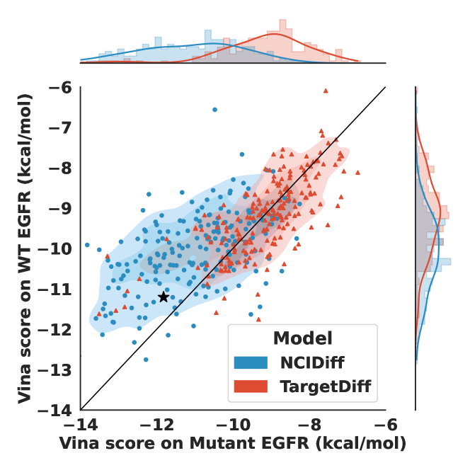
Figure 3: Scatter plot showing Vina scores of generated ligands from NCIDiff and TargetDiff, docked on either wild-type or mutant EGFR. The black star indicates the Vina scores of an original ligand from the retrieved complex.

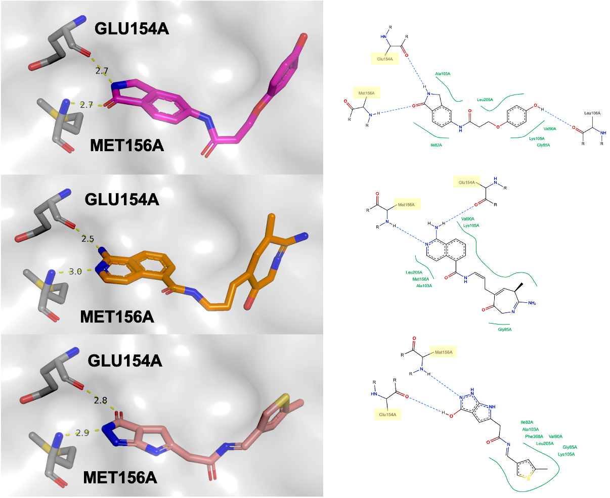
Figure 8: Examples of generated ligands that form two specific hydrogen bonds with the hinge region of ROCK1. Left: binding structures visualized by PyMOL (DeLano et al., 2002), Right: interaction profiles visualized by PoseEdit (Diedrich et al., 2023).

ROCK1 hinge binder design We aimed to design ligands that potentially bind to the hinge region of Rho-associated protein kinase 1 (ROCK1). As a kinase, the pocket of ROCK1 comprises an adenine-binding area at a hinge region that forms two hydrogen bonds with an adenine. From the ROCK1 pocket retrieved from (Li et al., 2012) (PDB ID: 3v8s), we inpaint two specific hydrogen bonds with specific atoms of two hinge residues — oxygen of Glu154 and nitrogen of Met156. We analyzed NCI patterns of 200 generated valid ligands by PLIP software; 59.5 % of generated ligands have accomplished forming two desired hydrogen bonds in the correct direction. In comparison, the ligands generated from TargetDiff achieved 41 %. Note that the baseline value is already over 40 %, implying that the hinge region is a well-exposed site that SBDD models can readily access. Nevertheless, focusing on the explicit hydrogen bonding pattern effectively increased the ratio of hinge binders. A few examples of NCIDiff-generated hinge binders are visualized in Figure 8.

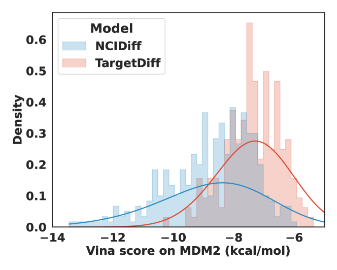
Figure 4: The evaluation of Vina scores obtained by docking generated ligands from NCIDiff and TargetDiff on MDM2.

p53/MDM2 inhibitor design We devised a task to mimic the protein-protein interface for ligand design. Our aim was to design ligands that can interfere with the p53 binding toward mouse double minute 2 homolog (MDM2), where MDM2 is a negative regulator of the p53 tumor suppressor (Chène, 2003). Using PLIP software, we used the complex structure reported in (Anil et al., 2013) (PDB ID: 4hfz) to extract the NCI pattern between the p53 and MDM2. The pattern is abundant in interactions, comprising 11 hydrophobic interactions, 4 hydrogen bonds, and 2 salt bridges. After generating 200 valid ligands by inpainting the extracted pattern, we profiled the interaction patterns of the generated ligands and analyzed the interaction similarities with the given pattern. We measured the Jaccard similarity coefficient between two interaction fingerprints by defining an interaction fingerprint as a flattened vector of a protein-side NCI pattern. As a result, ligands generated by our model achieved a mean value of 0.43 with a maximum value of 0.72. In contrast, generated ligands from TargetDiff exhibit a mean similarity of 0.00019 with a maximum value of 0.033, implying that generating a similar NCI pattern by chance is almost impossible. This substantiates the contribution of the NCI-guided strategy to mimicking the protein-protein interaction. Moreover, we analyzed Vina docking scores of generated ligands from each model. Figure 4 shows the resulting distribution, where NCIDiff and TargetDiff obtained mean docking scores of -8.77 and -7.38 kcal/mol, respectively. We note that the interaction pattern from protein-protein binding cannot serve as an answer for an optimal ligand design; still, the result implies that the given pattern is a good guess for generating ligands that can potentially form strong interactions with the target protein.

4 Limitations

This study emphasizes that NCIs should be considered by deep generative models for reliable structure-based drug design. However, predicting NCIs with high accuracy remains challenging due to their extremely sparse nature, resulting in room for improvement. For instance, the precision for $\pi$-$\pi$ stacking in NCIDiff-generated samples is 0.6, implying the extent of false positives in NCIs. Two possible approaches for advancements are of particular interest. First, recent studies on graph scalability, such as (Qin et al., 2023), have made it technically feasible for models to learn sparse and peaked distributions. Second, NCI types, such as salt bridges, are defined as a set of edges between every possible pair from a ligand motif’s atoms to a protein motif’s atoms in our method. This complexity makes it difficult for the model to generate such NCIs accurately. Considering NCIs as motif-to-motif interactions would reduce computational burden and complexity, thereby potentially improving NCIDiff’s performance.

5 Conclusion

In this work, we address the reliability of deep generative models for SBDD by focusing on NCIs that occur between a target protein and a ligand molecule. While non-covalent interactions are often overlooked despite their predominant role in ligand binding and universality across the diverse protein-ligand interactions, we propose NCIDiff, which adopts NCIs as an explicit generative objective in deep SBDD. Our strategy enables reference ligand-free generation, where previous methods relied on the ligand information of a given protein. Our experimental results reveal that generating non-covalent interactions not only induces the formation of more non-covalent interactions but also improves the reliability of generated ligand conformers. Lastly, by suggesting the NCI-guided generation scheme, we enjoy the effectiveness of ligand design tasks with specific objectives, implying the broad applicability of NCIDiff.

Impact Statement

This paper presents work whose goal is to advance the field of Machine Learning. There are many potential societal consequences of our work, none of which we feel must be specifically highlighted here.

Appendix A Node and Edge Features Used in NCIDiff

A.1 Node features

The input node features of ligand and protein atoms, ${h}^{\text{L}}_{i}$ and ${h}^{\text{P}}_{j}$, are used as described in the Supplementary Table 4. Each feature is represented as a one-hot vector of a corresponding category. Only an atom type is used for a ligand atom feature, while more informative features are used for a protein atom feature by concatenating every one-hot vector. The resulting dimensions of a ligand and a protein atom features are 10 and 40, respectively.

Ligand atom feature, ${h}^{\text{L}}_{i}$	Available list
Atom type	C, N, O, F, P, S, Cl, Br, I, $absorbing$ (one-hot)
Protein atom feature, ${h}^{\text{P}}_{j}$	Available list
Atom type	C, N, O, S, $else$ (one-hot)
Atom num H	0, 1, 2, 3, 4, 5, $else$ (one-hot)
Formal charge	-2, -1, 0, 1, 2 (one-hot)
Amino acid type	G, A, V, L, I, C, M, F, Y, W, P, S, T,
	Q, N, D, E, H, R, K, $else$ (one-hot)
Is $C_{\alpha}$?	0 or 1

Table 4:  The used node features of ligand and protein atoms with their available item lists to construct one-hot vectors. $absorbing$ indicates an absorbing type and $else$ is used when no items in the item list match the data type.

A.2 Edge features

The input intra and inter-edge features, ${e}^{\text{L}}_{ij}$, ${e}^{\text{P}}_{ij}$, and ${\mathbf{i}}_{ij}$, are used as described in the Supplementary Table 5. Each feature is represented as a one-hot vector of a corresponding category. For intra-edges of protein and ligand graphs, chemical bond types are used as features. For inter-edges between protein and ligands, NCI types are used as features. Note that the subject of directed NCI is set to protein; for instance, hydrogen bond donor type implies the donor is at the protein atom side. The resulting dimensions of intra and inter-edge features are 5 and 7, respectively.

Ligand and Protein intra-edge feature, ${e}^{\text{L}}_{ij}$ and ${e}^{\text{P}}_{ij}$	Available list
Bond type	Single, Double, Triple, Aromatic, absorbing (one-hot)
NCI inter-edge feature, ${\mathbf{i}}_{ij}$	Available list
NCI type	Salt bridge anion, Salt bridge cation,
	Hydrogen bond donor, Hydrogen bond acceptor,
	Hydrophobic interaction, $\pi$-$\pi$ stacking, absorbing (one-hot)

Table 5:  The used edge features of ligand and protein intra-edge and NCI inter-edge with their available item lists to construct one-hot vectors. $absorbing$ indicates an absorbing type and $else$ is used when no items in the item list match the data type.

Appendix B E(3)-equivariant dynamic interaction network

Our model receives a full bipartite graph of protein-ligand complex as an input, including a large number of edges. In order to reduce the computational cost and focus on the local atom environments, we devise an $E(3)$-equivariant dynamic interaction network act on protein-ligand heterograph. Thus, we design a neural network including dynamic sparse edge updates. Initially, messages are calculated as follows:

$$m_{ij}^{\text{P}} \leftarrow f_{\phi}^{\text{P}}(h_{i}^{\text{P}},h_{j}^{\text{P}},e_{ij}^{\text{P}},d_{ij}^{\text{P}}),$$ (16)

$$m_{ij}^{\text{L}} \leftarrow f_{\phi}^{\text{L}}(h_{i}^{\text{L}},h_{j}^{\text{L}},e_{ij}^{\text{L}},d_{ij}^{\text{L}}),$$

$$m_{ij}^{\text{I}} \leftarrow f_{\phi}^{\text{I}}(h_{i}^{\text{P}},h_{j}^{\text{L}},\mathbf{i}_{ij},d_{ij}^{\text{I}}),$$

then aggregated across neighboring nodes as follows:

$$m_{i}^{\text{P}} \leftarrow\sum_{j\in n_{t}(i)}{m_{ij}^{\text{P}}},$$ (17)

$$m_{i}^{\text{L}} \leftarrow\sum_{j\in n_{t}(i)}{m_{ij}^{\text{L}}},$$

$$m_{i}^{\text{I}},m_{j}^{\text{I}} \leftarrow\sum_{j\in n_{t}(i)}{m_{ij}^{\text{I}}},\sum_{i\in n_{t}(j)}{m_{ij}^{\text{I}}},$$

where $n_{t}(i)$ is a set of atom indices $\{j\}$ where the distance $d_{ij}<\gamma_{t}$. Note that the aggregation of $m_{ij}^{\text{I}}$ is asymmetric since the NCI edge is heterogeneous. For clarity, we use $i$ as an index for a protein atom and $j$ as an index for a ligand atom. Then, node features are updated as follows:

$$h_{i}^{\text{P}}\leftarrow f_{\psi}^{\text{P}}(h_{i}^{\text{P}},m_{i}^{\text{P}},m_{i}^{\text{I}}),$$ (18)

$$h_{j}^{\text{L}}\leftarrow f_{\psi}^{\text{L}}(h_{j}^{\text{L}},m_{j}^{\text{L}},m_{j}^{\text{I}}),$$

and ligand node positions are updated as follows:

$$x_{j}^{\text{L}}\leftarrow x_{j}^{\text{L}} +\sum_{i\in n_{t}(j)}f_{\tau}^{\text{I}}(m_{ij}^{\text{I}})\cdot(x_{i}^{\text{P}}-x_{j}^{\text{L}})+\sum_{k\in n_{t}(j)}f_{\tau}^{\text{L}}(m_{jk}^{\text{L}})\cdot(x_{k}^{\text{L}}-x_{j}^{\text{L}}),$$ (19)

and intra-edge features of protein and ligand bonds are updated as follows:

$$e_{ij}^{\text{P}} \leftarrow f_{\eta}^{\text{P}}(e_{ij}^{\text{P}}),$$ (20)

$$e_{ij}^{\text{L}} \leftarrow f_{\eta}^{\text{L}}(e_{ij}^{\text{L}}),$$

and inter-edge features of NCIs are updated as follows:

$$\mathbf{i}_{ij} \leftarrow f_{\eta}^{\text{I}}(\mathbf{i}_{ij}),$$ (21)

where $\phi$, $\tau$, and $\eta$ indicate learnable parameters.

We compute the radius edges for protein, ligand, and interaction edges in all layers to focus on closely placed atoms and reduce computational costs. Inspired by the dynamic radius graph from (Lu et al., 2024), we focus more on local structures in the final steps of the generative process while understanding the global structure in the early stages of generation. As described in Equation 11, we set the pair $(\gamma_{min},\gamma_{max})$ as (4, 8) for intra-edges and (6, 10) for inter-edges, conceiving that the distances of typical chemical bonds are under 2.0 $\mathrm{\text{\AA}}$ and NCIs are under 6.0 $\mathrm{\text{\AA}}$. Finally, the types of atoms, bonds, and NCIs are predicted as follows:

$$h_{i,\text{one-hot}}^{\text{L}} \sim\mathcal{C}\left(\text{softmax}(\text{MLP}({h}_{i}^{\text{L}}))\right),$$ (22)

$$e_{ij,\text{one-hot}}^{\text{L}} \sim\mathcal{C}\left(\text{softmax}(\text{MLP}(e_{ij}^{\text{L}}+e_{ji}^{\text{L}}))\right),$$

$$\mathbf{i}_{ij,\text{one-hot}} \sim\mathcal{C}\left(\text{softmax}(\text{MLP}(\mathbf{i}_{ij}))\right).$$

Appendix C Prior Distribution of the Number of Ligand Atoms for Given Pocket

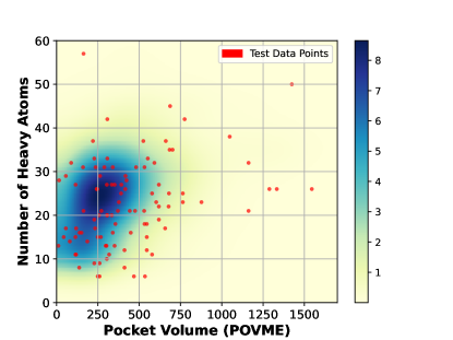
Figure 5: Distribution of the number of ligand heavy atoms and corresponding pocket volume measured by POVME. The red dots indicate the test data points.

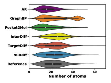
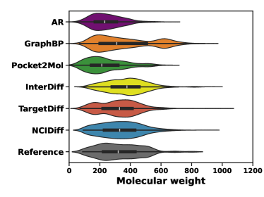
Figure 6: The plots show distributions of the numbers of atoms (Left) and molecular weights (Right) of generated ligands from various SBDD models and the test set ligands as a reference.

While previous diffusion generative models (Guan et al., 2023, 2024) utilized the farthest distance of protein atoms to estimate pocket size, these methods rely on pre-processed protein pockets based on a reference ligand. To achieve a reference ligand-free estimation of pocket volume, we used POcket Volume MEasurer 2 (POVME2) (Durrant et al., 2014). POVME2 analyzes the volume of a protein pocket by fitting a voxelized grid into the pocket. We ran POVME2 on the full training dataset with the default settings to obtain pocket volume estimates. Subsequently, we estimated the distribution of POVME to the number of atoms by applying a Gaussian to each data point. The Gaussian smearing standard deviation was set to 100, 3 for pocket volume and number of heavy atoms, respectively. During generation, we first measure the pocket volume and then obtain the given volume’s marginal distribution. Within the distribution, we randomly sample the number of atoms. Figure 5 depicts the distribution of the pocket volume and number of heavy atoms along with the test set marked.

The size of the molecule can highly affect the Vina score since larger molecules are likely to have half the low Vina score due to interference. As depicted in 6, it is clearly seen that NCIDiff prior atom sampling is done with a similar distribution with the reference molecule.

Appendix D Training and Sampling Details

Separate Nose schedule We use the same form of noise schedule from (Peng et al., 2023) which is in form of:

$$s =\frac{(s_{T}-s_{1})}{\text{sigmoid}(-w)-\text{sigmoid}(w)},$$ (23)

$$b =0.5\times(s_{1}+s_{T}-s),$$

$$\mkern 1.5mu\overline{\mkern-1.5mu\alpha\mkern-1.5mu}\mkern 1.5mu_{t} =s\times\text{sigmoid}\left(-w\left(\frac{2t}{T}-1\right)\right)+b,$$

where $s_{1}$, $s_{T}$, and $w$ are hyperparameters. To set the noise schedule in order of bond $\rightarrow$ NCI $\rightarrow$ atom, we choose the parameters as depicted on Table 6.

NCIDiff consists of 6 layers of $E(3)$-equivariant dynamic interaction networks with node and edge updates. For each layer of message passing, node processing, and edge processing layers, we use 2 layers of MLP with layer normalization. For stable training, we used a hyperbolic tangent activation function. A single neural network at each layer embeds the distance between each node and concatenates onto the message. The final prediction was done by a 2 layer MLP with layer normalization.

While training, we scale the loss for atom type, bond type, and NCI type to 100, 100, and 1,000 to match the scale of each loss. The model is trained using the Adam optimizer (Kingma & Ba, 2014), with an initial learning rate of $1e^{-3}$ and betas as $[0.95,0.99]$. Following (Guan et al., 2023), a small Gaussian noise of standard deviation $0.1$ was added to the atom coordinates of the protein atoms. The model was evaluated every 5 epochs with the validation set, and the learning rate was decreased to a factor of 0.8 if there was no improvement over 10 validation. We trained the model on a single NVIDIA A100 GPU, which took approximately 60 hours for convergence.

	Description	Value
Diffusion	Number of diffusion timestep	1000
	Atom type and position noise schedule	$(w,s_{1},s_{T})=(3,0.9999,0.0001)$ for $t\in[0,1000]$
	Bond type noise schedule	$(w,s_{1},s_{T})=(3,0.9999,0.001)$ for $t\in[0,600]$
	NCI type noise schedule	$(w,s_{1},s_{T})=(3,0.9999,0.001)$ for $t\in[0,800]$
Model	Embedding dimension of node features	96
	Embedding dimension of edge features	96
	Message dimension	96
	Timestep embedding dimension	32
	Number of layers	6
	$\gamma_{\text{min}}$ and $\gamma_{\text{max}}$ for intra edge	[4, 8]
	$\gamma_{\text{min}}$ and $\gamma_{\text{max}}$ for inter edge	[6, 10]
Train	Initial learning rate	0.001
	Weight decay	1e-16
	Batch size	64
Sampling	Number of RePaint iteration	4
	Bond distance guidance	0.03
	Interaction distance guidance	0.03
	Bond angle guidance	0.01

Table 6: Hyperparameter settings used in NCIDiff.

Appendix E NCI Inpainting Details

Here, we describe the algorithms for resampling with NCI inpainting using the RePaint method and for sampling the NCI pattern from pre-sampled ligands. These are used to generate ligands for NCIDiff^opt and NCIDiff^ref, as well as case studies.

Algorithm 1 Resampling with NCI inpainting using RePaint

  $I_{T}\leftarrow$ absorbing state

  for $t\in\{T,...,1\}$ do

     for $u\in\{1,...,U\}$ where U is the number of resampling steps do

        $I_{t-1}^{\textnormal{fix}}=I_{0}\mkern 1.5mu\overline{\mkern-1.5muQ\mkern-1.5mu}\mkern 1.5mu_{t-1}$

        $I_{t-1}^{\textnormal{gen}}=\frac{I_{t}Q_{t}^{\top}\odot\hat{I}_{0}\mkern 1.5mu\overline{\mkern-1.5muQ\mkern-1.5mu}\mkern 1.5mu_{t-1}}{\hat{I}_{0}\mkern 1.5mu\overline{\mkern-1.5muQ\mkern-1.5mu}\mkern 1.5mu_{t}I_{t}^{\top}}$

        $I_{t-1}=m^{\textnormal{fix}}\odot I^{\textnormal{fix}}_{t-1}+(1-m^{\textnormal{fix}})\odot I_{t-1}^{\textnormal{gen}}$

        if $u<U$ and $t>1$ then

           $I_{t}\sim\mathcal{C}(I_{t};I_{t-1}Q_{t})$

        end if

     end for

  end for

  return $I_{0}$

Algorithm 2 Sampling NCI pattern from pre-sampled ligands

  Input: $M$ pre-sampled ligands $\{L^{1},...,L^{M}\}$ and corresponding NCI patterns $\{I^{1},...,I^{M}\}$ for target protein $P$

  Output: sampled NCI pattern $I^{\text{opt}}$ from pre-sampled ligands

  Initialize $[S]_{jk}=0$ for protein atom index $j\in\{1,...,N_{P}\}$ and NCI type $k$

  for $m\in\{1,...,M\}$ do

     for $i\in\{1,...,N_{L}^{m}\}$ where $N_{L}^{m}$ is the number of atoms of $m$-th ligand $L^{m}$ do

        if $e_{I}^{(ij)}=k$ then

           $[S]_{jk}\leftarrow[S]_{jk}+1$

        end if

     end for

  end for

  $I^{\text{opt}}\leftarrow\textnormal{multinomial}_{k}(S)$

  return $I^{\text{opt}}$

Appendix F Bond and NCI Guidance Terms

We design guidance for bonds and NCIs to further improve our generations. The bond distance, bond angle, and interaction distance guidance for the $i$-th node are as follows:

$$\delta_{\text{BD},i} =-a_{\text{BD}}\nabla_{x_{t}}\sum_{j\in n_{\hat{L}_{0}}(i)}\biggl{[}\max(0,d_{ij}^{\text{L}}-d_{\text{BD}}^{\text{max}})+\max(0,d_{\text{BD}}^{\text{min}}-d_{ij}^{\text{L}})\biggr{]},$$ (24)

$$\delta_{\text{ID},i} =-a_{\text{ID}}\nabla_{x_{t}}\sum_{j\in n_{\hat{L}_{0}}(i)}\sum_{\kappa\in\text{NCI}}\biggl{[}\max(0,d_{ij}^{\text{I}}-d_{\text{ID},\kappa}^{\text{max}})+\max(0,d_{\text{ID},\kappa}^{\text{min}}-d_{ij}^{\text{I}})\biggr{]},$$

$$\delta_{\text{BA},i} =-a_{\text{BA}}\nabla_{x_{t}}\sum_{\begin{subarray}{c}i\in n_{\hat{L}_{0}}(j),\\ k\in n_{\hat{L}_{0}}(j),\\ i\neq k\end{subarray}}\biggl{[}\max(0,\rho^{\text{min}}-d_{ik}^{\text{L}})\biggr{]},$$

where $a_{\text{BD}}$, $a_{\text{ID}}$, and $a_{\text{BA}}$ are scaling coefficients for each guidance term, which the values provided in Table 6. The minimum distance for bond angle guidance, $\rho^{\text{min}}$ is calculated from the law of cosines as follows:

$$\rho^{\text{min}} =d_{\text{BD}}^{\text{min}}\sqrt{2\cdot(1-\text{cos}\angle{}^{\text{min}})},$$ (25)

where $\angle^{\text{min}}$ was set to 90$\mathrm{\SIUnitSymbolDegree}$ to prevent high angle strains.

Here, $n_{\hat{L}_{0}}(i)$ denotes the indices of bond-connected nodes to $i$-th node in $\hat{L}_{0}$. In practice, $d_{\text{BD}}^{\text{min}}$, $d_{\text{BD}}^{\text{max}}$ are set to 1.2 and 1.9, respectively, since most covalent bonds in typical small molecules fall into this range. For NCI distance guidance, we set different $d_{\text{ID},\kappa}^{\text{min}}$ and $d_{\text{ID},\kappa}^{\text{max}}$ for each NCI type, $\kappa$, as depicted in Table 7.

NCI type, $\kappa$	$d_{\text{ID},\kappa}^{\text{min}}$	$d_{\text{ID}_{\kappa}}^{\text{max}}$
salt bridge	2.0 $\mathrm{\text{\AA}}$	5.5 $\mathrm{\text{\AA}}$
hydrogen bond	2.0 $\mathrm{\text{\AA}}$	4.1 $\mathrm{\text{\AA}}$
hydrophobic interaction	2.0 $\mathrm{\text{\AA}}$	4.0 $\mathrm{\text{\AA}}$
$\pi$-$\pi$ interaction	2.0 $\mathrm{\text{\AA}}$	5.5 $\mathrm{\text{\AA}}$

Table 7: Parameters for interaction distance guidance terms.

Appendix G Examples of NCIDiff-generated ligands

Figure 7: Examples of NCIDiff-generated molecules with lower Vina docking scores on pocket $\text{3HY9}\_\text{B}(\textbf{Up})$ and $\text{4QLK}\_\text{A}$ (Down) visualized by PyMOL (DeLano et al., 2002).

Appendix H Examples of ROCK1 hinge binders and their interaction profiles

References

- Abramson et al. (2024) Abramson, J., Adler, J., Dunger, J., Evans, R., Green, T., Pritzel, A., Ronneberger, O., Willmore, L., Ballard, A. J., Bambrick, J., et al. Accurate structure prediction of biomolecular interactions with alphafold 3. Nature, pp. 1–3, 2024.
- Achiam et al. (2023) Achiam, J., Adler, S., Agarwal, S., Ahmad, L., Akkaya, I., Aleman, F. L., Almeida, D., Altenschmidt, J., Altman, S., Anadkat, S., et al. Gpt-4 technical report. arXiv preprint arXiv:2303.08774, 2023.
- Anciukevičius et al. (2023) Anciukevičius, T., Xu, Z., Fisher, M., Henderson, P., Bilen, H., Mitra, N. J., and Guerrero, P. Renderdiffusion: Image diffusion for 3d reconstruction, inpainting and generation. In Proceedings of the IEEE/CVF Conference on Computer Vision and Pattern Recognition, pp. 12608–12618, 2023.
- Anderson (2003) Anderson, A. C. The process of structure-based drug design. Chemistry & biology, 10(9):787–797, 2003.
- Anil et al. (2013) Anil, B., Riedinger, C., Endicott, J. A., and Noble, M. E. The structure of an mdm2–nutlin-3a complex solved by the use of a validated mdm2 surface-entropy reduction mutant. Acta Crystallographica Section D: Biological Crystallography, 69(8):1358–1366, 2013.
- Austin et al. (2021) Austin, J., Johnson, D. D., Ho, J., Tarlow, D., and Van Den Berg, R. Structured denoising diffusion models in discrete state-spaces. Advances in Neural Information Processing Systems, 34:17981–17993, 2021.
- Bhujbal et al. (2022) Bhujbal, S. P., Kim, H., Bae, H., and Hah, J.-M. Design and synthesis of aminopyrimidinyl pyrazole analogs as plk1 inhibitors using hybrid 3d-qsar and molecular docking. Pharmaceuticals, 15(10):1170, 2022.
- Bickerton et al. (2012) Bickerton, G. R., Paolini, G. V., Besnard, J., Muresan, S., and Hopkins, A. L. Quantifying the chemical beauty of drugs. Nature chemistry, 4(2):90–98, 2012.
- Chène (2003) Chène, P. Inhibiting the p53–mdm2 interaction: an important target for cancer therapy. Nature reviews cancer, 3(2):102–109, 2003.
- de Freitas & Schapira (2017) de Freitas, R. F. and Schapira, M. A systematic analysis of atomic protein–ligand interactions in the pdb. Medchemcomm, 8(10):1970–1981, 2017.
- DeLano et al. (2002) DeLano, W. L. et al. Pymol: An open-source molecular graphics tool. CCP4 Newsl. Protein Crystallogr, 40(1):82–92, 2002.
- Diedrich et al. (2023) Diedrich, K., Krause, B., Berg, O., and Rarey, M. Poseedit: Enhanced ligand binding mode communication by interactive 2d diagrams. Journal of Computer-Aided Molecular Design, 37(10):491–503, 2023.
- Durrant et al. (2014) Durrant, J. D., Votapka, L., Sørensen, J., and Amaro, R. E. Povme 2.0: an enhanced tool for determining pocket shape and volume characteristics. Journal of chemical theory and computation, 10(11):5047–5056, 2014.
- Ertl & Schuffenhauer (2009) Ertl, P. and Schuffenhauer, A. Estimation of synthetic accessibility score of drug-like molecules based on molecular complexity and fragment contributions. Journal of cheminformatics, 1:1–11, 2009.
- Feng et al. (2024) Feng, W., Wang, L., Lin, Z., Zhu, Y., Wang, H., Dong, J., Bai, R., Wang, H., Zhou, J., Peng, W., et al. Generation of 3d molecules in pockets via a language model. Nature Machine Intelligence, pp. 1–12, 2024.
- Francoeur et al. (2020) Francoeur, P. G., Masuda, T., Sunseri, J., Jia, A., Iovanisci, R. B., Snyder, I., and Koes, D. R. Three-dimensional convolutional neural networks and a cross-docked data set for structure-based drug design. Journal of chemical information and modeling, 60(9):4200–4215, 2020.
- Guan et al. (2023) Guan, J., Qian, W. W., Peng, X., Su, Y., Peng, J., and Ma, J. 3d equivariant diffusion for target-aware molecule generation and affinity prediction. arXiv preprint arXiv:2303.03543, 2023.
- Guan et al. (2024) Guan, J., Zhou, X., Yang, Y., Bao, Y., Peng, J., Ma, J., Liu, Q., Wang, L., and Gu, Q. Decompdiff: diffusion models with decomposed priors for structure-based drug design. arXiv preprint arXiv:2403.07902, 2024.
- Harris et al. (2023) Harris, C., Didi, K., Jamasb, A., Joshi, C., Mathis, S., Lio, P., and Blundell, T. Posecheck: Generative models for 3d structure-based drug design produce unrealistic poses. In NeurIPS 2023 Generative AI and Biology (GenBio) Workshop, 2023.
- Ho et al. (2020) Ho, J., Jain, A., and Abbeel, P. Denoising diffusion probabilistic models. Advances in neural information processing systems, 33:6840–6851, 2020.
- Jumper et al. (2021) Jumper, J., Evans, R., Pritzel, A., Green, T., Figurnov, M., Ronneberger, O., Tunyasuvunakool, K., Bates, R., Žídek, A., Potapenko, A., et al. Highly accurate protein structure prediction with alphafold. Nature, 596(7873):583–589, 2021.
- Kingma & Ba (2014) Kingma, D. P. and Ba, J. Adam: A method for stochastic optimization. arXiv preprint arXiv:1412.6980, 2014.
- Li et al. (2012) Li, R., Martin, M. P., Liu, Y., Wang, B., Patel, R. A., Zhu, J.-Y., Sun, N., Pireddu, R., Lawrence, N. J., Li, J., et al. Fragment-based and structure-guided discovery and optimization of rho kinase inhibitors. Journal of medicinal chemistry, 55(5):2474–2478, 2012.
- Lin et al. (2022) Lin, H., Huang, Y., Liu, M., Li, X., Ji, S., and Li, S. Z. Diffbp: Generative diffusion of 3d molecules for target protein binding. arXiv preprint arXiv:2211.11214, 2022.
- Liu et al. (2022) Liu, M., Luo, Y., Uchino, K., Maruhashi, K., and Ji, S. Generating 3d molecules for target protein binding. arXiv preprint arXiv:2204.09410, 2022.
- Lu et al. (2024) Lu, W., Zhang, J., Huang, W., Zhang, Z., Jia, X., Wang, Z., Shi, L., Li, C., Wolynes, P. G., and Zheng, S. Dynamicbind: predicting ligand-specific protein-ligand complex structure with a deep equivariant generative model. Nature Communications, 15(1):1071, 2024.
- Lugmayr et al. (2022) Lugmayr, A., Danelljan, M., Romero, A., Yu, F., Timofte, R., and Van Gool, L. Repaint: Inpainting using denoising diffusion probabilistic models. In Proceedings of the IEEE/CVF conference on computer vision and pattern recognition, pp. 11461–11471, 2022.
- Luo et al. (2021) Luo, S., Guan, J., Ma, J., and Peng, J. A 3d generative model for structure-based drug design. Advances in Neural Information Processing Systems, 34:6229–6239, 2021.
- Méndez-Lucio et al. (2021) Méndez-Lucio, O., Ahmad, M., del Rio-Chanona, E. A., and Wegner, J. K. A geometric deep learning approach to predict binding conformations of bioactive molecules. Nature Machine Intelligence, 3(12):1033–1039, 2021.
- Moon et al. (2022) Moon, S., Zhung, W., Yang, S., Lim, J., and Kim, W. Y. Pignet: a physics-informed deep learning model toward generalized drug–target interaction predictions. Chemical Science, 13(13):3661–3673, 2022.
- Moon et al. (2024) Moon, S., Hwang, S.-Y., Lim, J., and Kim, W. Y. Pignet2: a versatile deep learning-based protein–ligand interaction prediction model for binding affinity scoring and virtual screening. Digital Discovery, 2024.
- O’Boyle et al. (2011) O’Boyle, N. M., Banck, M., James, C. A., Morley, C., Vandermeersch, T., and Hutchison, G. R. Open babel: An open chemical toolbox. Journal of cheminformatics, 3:1–14, 2011.
- Peng et al. (2022) Peng, X., Luo, S., Guan, J., Xie, Q., Peng, J., and Ma, J. Pocket2mol: Efficient molecular sampling based on 3d protein pockets. In International Conference on Machine Learning, pp. 17644–17655. PMLR, 2022.
- Peng et al. (2023) Peng, X., Guan, J., Liu, Q., and Ma, J. Moldiff: addressing the atom-bond inconsistency problem in 3d molecule diffusion generation. arXiv preprint arXiv:2305.07508, 2023.
- Qian et al. (2024) Qian, H., Huang, W., Tu, S., and Xu, L. Kgdiff: towards explainable target-aware molecule generation with knowledge guidance. Briefings in Bioinformatics, 25(1):bbad435, 2024.
- Qin et al. (2023) Qin, Y., Vignac, C., and Frossard, P. Sparse training of discrete diffusion models for graph generation. arXiv preprint arXiv:2311.02142, 2023.
- Ragoza et al. (2022) Ragoza, M., Masuda, T., and Koes, D. R. Generating 3d molecules conditional on receptor binding sites with deep generative models. Chemical science, 13(9):2701–2713, 2022.
- Ramesh et al. (2021) Ramesh, A., Pavlov, M., Goh, G., Gray, S., Voss, C., Radford, A., Chen, M., and Sutskever, I. Zero-shot text-to-image generation. In International conference on machine learning, pp. 8821–8831. Pmlr, 2021.
- Salentin et al. (2015) Salentin, S., Schreiber, S., Haupt, V. J., Adasme, M. F., and Schroeder, M. Plip: fully automated protein–ligand interaction profiler. Nucleic acids research, 43(W1):W443–W447, 2015.
- Satorras et al. (2021) Satorras, V. G., Hoogeboom, E., and Welling, M. E (n) equivariant graph neural networks. In International conference on machine learning, pp. 9323–9332. PMLR, 2021.
- Schneuing et al. (2022) Schneuing, A., Du, Y., Harris, C., Jamasb, A., Igashov, I., Du, W., Blundell, T., Lió, P., Gomes, C., Welling, M., et al. Structure-based drug design with equivariant diffusion models. arXiv preprint arXiv:2210.13695, 2022.
- Seo & Kim (2023) Seo, S. and Kim, W. Y. Pharmaconet: Accelerating large-scale virtual screening by deep pharmacophore modeling. In NeurIPS 2023 Workshop on New Frontiers of AI for Drug Discovery and Development, 2023.
- Shen et al. (2022) Shen, C., Zhang, X., Deng, Y., Gao, J., Wang, D., Xu, L., Pan, P., Hou, T., and Kang, Y. Boosting protein–ligand binding pose prediction and virtual screening based on residue–atom distance likelihood potential and graph transformer. Journal of Medicinal Chemistry, 65(15):10691–10706, 2022.
- Sogabe et al. (2013) Sogabe, S., Kawakita, Y., Igaki, S., Iwata, H., Miki, H., Cary, D. R., Takagi, T., Takagi, S., Ohta, Y., and Ishikawa, T. Structure-based approach for the discovery of pyrrolo [3, 2-d] pyrimidine-based egfr t790m/l858r mutant inhibitors. ACS medicinal chemistry letters, 4(2):201–205, 2013.
- Trott & Olson (2010) Trott, O. and Olson, A. J. Autodock vina: improving the speed and accuracy of docking with a new scoring function, efficient optimization, and multithreading. Journal of computational chemistry, 31(2):455–461, 2010.
- van den Burg & Williams (2021) van den Burg, G. and Williams, C. On memorization in probabilistic deep generative models. Advances in Neural Information Processing Systems, 34:27916–27928, 2021.
- Verma et al. (2010) Verma, J., Khedkar, V. M., and Coutinho, E. C. 3d-qsar in drug design-a review. Current topics in medicinal chemistry, 10(1):95–115, 2010.
- Vignac et al. (2023) Vignac, C., Osman, N., Toni, L., and Frossard, P. Midi: Mixed graph and 3d denoising diffusion for molecule generation. In Joint European Conference on Machine Learning and Knowledge Discovery in Databases, pp. 560–576. Springer, 2023.
- Wu et al. (2024) Wu, P., Du, H., Yan, Y., Lee, T.-Y., Bai, C., and Wu, S. Guided diffusion for molecular generation with interaction prompt. Briefings in Bioinformatics, 25(3):bbae174, 2024.
- Zhou et al. (2012) Zhou, P., Huang, J., and Tian, F. Specific noncovalent interactions at protein-ligand interface: implications for rational drug design. Current medicinal chemistry, 19(2):226–238, 2012.
- Zhung et al. (2024) Zhung, W., Kim, H., and Kim, W. Y. 3d molecular generative framework for interaction-guided drug design. Nature Communications, 15(1):2688, 2024.