Gaussian Mixture Model with Rare Events

Abstract

We study here a Gaussian Mixture Model (GMM) with rare events data. In this case, the commonly used Expectation-Maximization (EM) algorithm exhibits extremely slow numerical convergence rate. To theoretically understand this phenomenon, we formulate the numerical convergence problem of the EM algorithm with rare events data as a problem about a contraction operator. Theoretical analysis reveals that the spectral radius of the contraction operator in this case could be arbitrarily close to 1 asymptotically. This theoretical finding explains the empirical slow numerical convergence of the EM algorithm with rare events data. To overcome this challenge, a Mixed EM (MEM) algorithm is developed, which utilizes the information provided by partially labeled data. As compared with the standard EM algorithm, the key feature of the MEM algorithm is that it requires additionally labeled data. We find that MEM algorithm significantly improves the numerical convergence rate as compared with the standard EM algorithm. The finite sample performance of the proposed method is illustrated by both simulation studies and a real-world dataset of Swedish traffic signs.

Keywords: Rare Events Data, Gaussian Mixture Model, Expectation-Maximum Algorithm, Partial Labeled Data, Unsupervised Learning

1 Introduction

In this study, we investigate a problem related to the analysis of rare events data. Rare events data are defined as a type of data with a binary response ($Y\in\mathbb{R}^{1}$) and feature vector ($X\in\mathbb{R}^{p}$). Furthermore, we require that the probability of the response belonging to one particular class (e.g., $Y=1$) is extremely small. For convenience, we refer to this class (i.e., the class with $Y=1$) as the minor class, representing rare events, and the other class (i.e., the class with $Y=0$) as the major class, representing non-rare events. To theoretically model the phenomenon of rare events, we adopt the idea proposed by Wang (2020) and assume that the response probability for the minor class shrinks towards 0 as the sample size diverges to infinity. Note that the rare event studied here is not an extreme value event. In this work, a rare event refers to a random event generated by a binary distribution, where the response probability for one particular class is extremely small. Note that the binary distribution is a discrete distribution. In contrast, an extreme value event is typically referred to a random event generated by one particular type of extreme value distribution (e.g., Pareto distribution), which is often a continuous distribution (Kotz and Nadarajah, 2000).

Rare events data are commonly encountered in practical scenarios. For example, consider an online banking system that generates large volumes of daily transaction records. Each transaction record can be treated as a sample and classified into two classes based on whether it is related to fraud or not. Naturally, the probability of a transaction record being a fraud is extremely low, making fraud records rare events (Krivko, 2010; Sanz et al., 2015). Another example involves computed tomography (CT) scans in medical imaging studies (Gu et al., 2019; Polat, 2022). The objective here is to identify specific disease regions within high-resolution CT images. A common approach is to treat each pixel as a sample (Heimann et al., 2009; Mansoor et al., 2015). Subsequently, positive samples represent pixels associated with disease, while negative samples represent pixels unrelated to disease. Often, the proportion of disease-related pixels (i.e., positive samples) is extremely small, thus classifying them as rare events. Other examples of rare events related data include drug discovery (Amaro et al., 2018; Korkmaz, 2020), data leakage prevention (Sigholm and Raciti, 2012), and intrusion detection in the cybersecurity scenario (Qian et al., 2008; Gulati et al., 2013; Bagui and Li, 2021). For a comprehensive summary, we refer to Chandola et al. (2009) and Pimentel et al. (2014).

The statistical analysis of rare events data differs significantly from that of regular data. First, rare events are rare and thus contain more valuable information than non-rare events. For example, in a standard logistic regression model, Wang (2020) discovered that the statistical efficiency of the maximum likelihood estimator (MLE) is predominantly influenced by the sample size of rare events. In contrast, the sample size of non-rare events plays a considerably less significant role. Consequently, direct implementation of the standard maximum likelihood estimation results in unnecessarily high computational costs and additional storage requirements, particularly for datasets with massive sizes. In this regard, various undersampling methods have been developed to reduce unnecessary computation (Nguyen et al., 2012; Wang, 2020; Wang et al., 2021). These methods are not limited to logistic regression and have been applied to decision trees (Liu et al., 2009; Pozo et al., 2021), support vector machine (Tang et al., 2009; Bao et al., 2016) and many others (Spelmen and Porkodi, 2018; Mohammed et al., 2020). Distributed computation methods with similar objectives have also been developed by Triguero et al. (2015, 2016) and Duan et al. (2020).

Despite significant progress in the literature on rare events data analysis, existing methods often share a common limitation: the requirement for fully labeled datasets. This implies that the binary response $Y$ for each sample must be accurately observed and cannot be latent or missing. Consequently, a statistical learning model can be constructed to relate the binary response $Y$ to the feature vector $X$. However, this is not always feasible in practical applications. In fact, for many real-world applications, the collection of the feature vector $X$ is automated using well-designed hardware and software, resulting in relatively low data collection costs. On the other hand, obtaining the response $Y$ often relies on human effort and is considerably more expensive. For instance, in the case of obtaining a nodule mask for a lung CT image, it usually involves hiring two or more experienced radiologists to manually annotate the nodule location in a two-stage process (Setio et al., 2017). This makes the problem of unsupervised and semi-supervised learning a problem of great importance.

As our first attempt, we investigate one of the most commonly used unsupervised learning methods, the Gaussian Mixture Model (GMM). The GMM is a model of fundamental importance that has been extensively studied in the literature (Boldea and Magnus, 2009; McLachlan et al., 2019). The Expectation-Maximization (EM) algorithm is commonly employed for GMM estimation (Wu, 1983; Xu and Jordan, 1996), and its theoretical properties have been extensively examined. Specifically, Dempster et al. (1977) first introduced the general form of the EM algorithm and demonstrated that the likelihood value does not decrease with each iteration. Wu (1983) rigorously proved that the estimator obtained by the EM algorithm numerically converges to the MLE under appropriate regularity conditions. Xu and Jordan (1996) investigated the numerical convergence rate of the EM algorithm for GMM and established an interesting relationship between the EM algorithm and gradient ascent methods. They showed that the conditional number of the EM algorithm is always smaller than that of the gradient ascent algorithm, suggesting that the numerical convergence speed of the EM algorithm is not worse. Xu et al. (2016) and Daskalakis et al. (2017) conducted a global analysis of the EM algorithm for the mixture of two Gaussians from random initialization. However, all these theoretical results were obtained under the assumption of non-rare events data. In contrast, it has been widely observed that the standard EM algorithm exhibits painfully slow convergence rates for GMM with rare events. This intriguing phenomenon remains unexplained by existing theories. Naim and Gildea (2012) have provided simulation-based arguments, but no rigorously asymptotic theory has been developed in this regard. The aim of this study is to fill this important theoretical gap.

To address this problem, we formulate the EM algorithm for the GMM with rare events as an iterative algorithm governed by a contraction operator. The convergence rate of this algorithm is predominantly determined by the spectral radius of the contraction operator. Our theoretical studies reveal that, as the percentage of the rare events approaches 0, the spectral radius of the contraction operator could be arbitrarily close to 1 asymptotically, causing the numerical convergence of the EM algorithm extremely slow. Our simulation studies also confirm that the spectral radius of the contraction operator approaches 1 as the response probability tends to 0. This indicates that the numerical convergence rate of the standard EM algorithm can be extremely slow for a GMM with rare events. To overcome this challenge, it becomes necessary to obtain a subsample of data with accurately observed labels. By doing so, we aim to significantly enhance the numerical convergence properties of the EM algorithm. Consequently, we propose a Mixed EM (MEM) algorithm and meticulously examine its numerical convergence properties. Our findings demonstrate that the numerical convergence properties of the EM algorithm can be improved when the percentage of labeled data is carefully selected. Extensive simulation studies are presented in this paper to demonstrate the numerical convergence properties of these two algorithms.

In summary, we aim to make the following contributions to the existing literature. First, we theoretically prove that the numerical convergence rate of the standard EM algorithm can be extremely slow for a GMM with rare events. Second, to fix the problem, an MEM algorithm is developed by using a partially labeled dataset. We theoretically prove that the numerical convergence rate of this algorithm can be much faster than that of the standard EM algorithm. These theoretical findings are further verified by extensive numerical studies. The technical details are given in our Appendix A.1–A.2, which is heavily involved but fairly standard. The remainder of this paper is organized as follows. Section 2 introduces the model setting for unsupervised learning and the numerical convergence analysis of the standard EM algorithm. Section 3 presents the model settings of semi-supervised learning and a numerical convergence analysis of the MEM algorithm. Numerical studies are given in Section 4. Moreover, the application of the proposed methods is then illustrated using the Swedish Traffic Signs dataset. Finally, the article concludes with a brief discussion in Section 5. All technical details are provided in the Appendices.

2 Unsupervised Learning

2.1 Problem Setup

Assume a total of $N$ observations are indexed by $1\leq i\leq N$. The $i$th observation is denoted as $X_{i}\in\mathbb{R}^{p}$, which is a $p$-dimensional random vector. To model the random behavior of $X_{i}$, a GMM is considered (McLachlan and Basford, 1988; Boldea and Magnus, 2009; McNicholas, 2016). Specifically, we assume a latent binary random variable $Y_{i}\in\{0,1\}$ with $P(Y_{i}=1)=\alpha$ for some response probability $0<\alpha<1$. Next, we assume that $X_{i}$ follows a normal distribution with mean $\mu_{0}=(\mu_{0,j})\in\mathbb{R}^{p}$ and covariance $\Sigma_{0}=(\sigma_{0,j_{1}j_{2}})\in\mathbb{R}^{p\times p}$ if $Y_{i}=0$. Otherwise, we assume another normal distribution for $X_{i}$ with mean $\mu_{1}=(\mu_{1,j})\in\mathbb{R}^{p}$ and covariance $\Sigma_{1}=(\sigma_{1,j_{1}j_{2}})\in\mathbb{R}^{p\times p}$. Suppose $A=(A_{ij})\in\mathbb{R}^{p\times p}$ be an arbitrary square matrix of $p\times p$ dimensions. Then, we define $\mathrm{vec}(A)=(A_{ij}:1\leq i,j\leq p)\in\mathbb{R}^{p^{2}}$. Moreover, if $A$ is a symmetric matrix in the sense that $A_{ij}=A_{ji}$ for $1\leq i\leq j\leq p$, we define the half-vec operator $\mathrm{vech}(A)=(A_{ij}:1\leq i\leq j\leq p)\in\mathbb{R}^{p(p+1)/2}$ (Boldea and Magnus, 2009). In this case, there should exist a unique matrix $D\in\mathbb{R}^{p^{2}\times p(p+1)/2}$ such that $D\mathrm{vech}(A)=\mathrm{vec}(A)$. We then refer to $D$ as a duplication matrix. See Magnus (1988), Boldea and Magnus (2009), and Magnus and Neudecker (2019) for further details. We write $\theta=(\alpha,\mu_{0}^{\top},\mathrm{vech}(\Sigma_{0})^{\top},\mu_{1}^{\top},\mathrm{vech}(\Sigma_{1})^{\top})^{\top}\in\mathbb{R}^{q}$ as our interested parameter vector with $q=p^{2}+3p+1$. Then, the probability density function of the GMM can be written as $f_{\theta}(x)=\alpha\phi_{\mu_{1},\Sigma_{1}}(x)+(1-\alpha)\phi_{\mu_{0},\Sigma_{0}}(x)$, where $\phi_{\mu,\Sigma}(x)=(|2\pi\Sigma|)^{-1/2}\exp\{-(x-\mu)^{\top}\Sigma^{-1}(x-\mu)/2\}$ is the probability density function of a multivariate normal distribution with mean $\mu\in\mathbb{R}^{p}$ and covariance $\Sigma\in\mathbb{R}^{p\times p}$ (McLachlan and Basford, 1988).

For a classical GMM, we should have $\alpha\in(0,1)$ as a fixed parameter in the sense that it does not vanish as the sample size increases. Under this setup, we should have the expected sample size ratio $\color[rgb]{0,0,0}E(N_{1})/N=\alpha\nrightarrow 0$ as $N\to\infty$, where $N_{1}=\sum_{i=1}^{N}Y_{i}$. Unfortunately, this classical setup is inappropriate for applications involving rare events. In this case, one of the two latent classes (e.g., the class with $Y_{i}=1$) is considered as the minor class with a mixing probability $\alpha\to 0$ as $N\to\infty$, and the other latent class (e.g., the class with $Y_{i}=0$) is considered as the major class with a mixing probability $1-\alpha\to 1$ as $N\to\infty$. Consequently, the sample size associated with the minor class (e.g., $N_{1}$) is significantly smaller than that of the major class (e.g., $N_{0}=N-N_{1}$) in the sense that $N_{1}/N\to_{p}0$ as $N\to\infty$. It is worthwhile mentioning that $\alpha$ cannot be excessively small either. Otherwise, the sample size of the minor latent class (i.e., $N_{1}$) might shrink towards 0. Consequently, the parameters associated with the minor class (i.e., $\mu_{1}$ and $\Sigma_{1}$) cannot be consistently estimated even if class label $Y_{i}$s are given. In this case, no meaningful asymptotic theory can be established. For the sake of asymptotic theory development, we do need to assume that $E(N_{1})\to\infty$ as $N\to\infty$. This further requires that $N\alpha\to\infty$ as $N\to\infty$. Therefore, throughout the remainder of this article, we always assume that (1) $\alpha\to 0$ and (2) $N\alpha\to\infty$ as $N\to\infty$; see Wang (2020), Wang et al. (2021) and Li et al. (2023) for further discussion. These two assumptions are called the rare events assumptions.

2.2 The EM Algorithm

Next, we consider how to compute the MLE for the GMM. The log-likelihood function is given as follows

$$\mathcal{L}(\theta)=\sum_{i=1}^{N}\log f_{\theta}(X_{i}).$$ (1)

Subsequently, we can obtain the MLE as $\widehat{\theta}=(\widehat{\alpha},\widehat{\mu}_{0}^{\top},\mathrm{vech}(\widehat{\Sigma}_{0})^{\top},\widehat{\mu}_{1}^{\top},\mathrm{vech}(\widehat{\Sigma}_{1})^{\top})^{\top}=\mbox{argmax}_{\theta}$ $\mathcal{L}(\theta)$. To compute the MLE, a classical EM algorithm can be used (Dempster et al., 1977; Biernacki et al., 2003). In the past literature, a standard EM algorithm was often motivated by the method of complete log-likelihood, where the latent class label $Y_{i}$s are pretended to be known. In this study, we present another interesting perspective, where the EM algorithm is inspired by the gradient condition of the log-likelihood function without knowing the latent class labels.

Specifically, define $\dot{\mathcal{L}}(\theta)=(\dot{\mathcal{L}}_{\alpha}(\theta),\dot{\mathcal{L}}_{\mu_{0}}(\theta)^{\top},\dot{\mathcal{L}}_{\Sigma_{0}}(\theta)^{\top},\dot{\mathcal{L}}_{\mu_{1}}(\theta)^{\top},\dot{\mathcal{L}}_{\Sigma_{1}}(\theta)^{\top})^{\top}\in\mathbb{R}^{q}$, where $\dot{\mathcal{L}}_{\alpha}(\theta)=\partial\mathcal{L}(\theta)/\partial\alpha\in\mathbb{R}$, $\dot{\mathcal{L}}_{\mu_{k}}(\theta)=\partial\mathcal{L}(\theta)/\partial\mu_{k}\in\mathbb{R}^{p}$ and $\dot{\mathcal{L}}_{\Sigma_{k}}(\theta)=\partial\mathcal{L}(\theta)/\partial\mathrm{vech}(\Sigma_{k})\in\mathbb{R}^{p(p+1)/2}$ with $k\in\{0,1\}$. Recall that $\widehat{\theta}$ denotes the MLE. Consequently, we should have a gradient condition as $\dot{\mathcal{L}}(\widehat{\theta})=0$. This suggests a set of estimation equations as $\widehat{\alpha}=\mathcal{F}_{\alpha}(\widehat{\theta})$, $\widehat{\mu}_{k}=\mathcal{F}_{\mu_{k}}(\widehat{\theta})$ and $\mathrm{vech}(\widehat{\Sigma}_{k})=\mathcal{F}_{\Sigma_{k}}(\widehat{\theta})$ with $k\in\{0,1\}$. Here $\mathcal{F}(\theta)=$ $(\mathcal{F}_{\alpha}(\theta),\mathcal{F}_{\mu_{0}}(\theta)^{\top},\mathcal{F}_{\Sigma_{0}}(\theta)^{\top}$, $\mathcal{F}_{\mu_{1}}(\theta)^{\top},\mathcal{F}_{\Sigma_{1}}(\theta)^{\top})^{\top}\in\mathbb{R}^{q}$ is a mapping function, where

$$\mathcal{F}_{\alpha}(\theta)=N^{-1}\sum_{i=1}^{N}\pi_{i}\in\mathbb{R},\ \mathcal{F}_{\mu_{0}}(\theta)=\Big{\{}\sum_{i=1}^{N}(1-\pi_{i})\Big{\}}^{-1}\sum_{i=1}^{N}(1-\pi_{i})X_{i}\in\mathbb{R}^{p},$$

$$\mathcal{F}_{\Sigma_{0}}(\theta)=\Big{\{}\sum_{i=1}^{N}(1-\pi_{i})\Big{\}}^{-1}\sum_{i=1}^{N}\Big{(}1-\pi_{i}\Big{)}\mathrm{vech}\Big{\{}\Big{(}X_{i}-\mu_{0}\Big{)}\Big{(}X_{i}-\mu_{0}\Big{)}^{\top}\Big{\}}\in\mathbb{R}^{\frac{(p+1)p}{2}},$$

$$\mathcal{F}_{\mu_{1}}(\theta)=\Big{(}\sum_{i=1}^{N}\pi_{i}\Big{)}^{-1}\sum_{i=1}^{N}\pi_{i}X_{i}\in\mathbb{R}^{p},$$ (2)

$$\mathcal{F}_{\Sigma_{1}}(\theta)=\Big{(}\sum_{i=1}^{N}\pi_{i}\Big{)}^{-1}\sum_{i=1}^{N}\pi_{i}\mathrm{vech}\Big{\{}\Big{(}X_{i}-\mu_{1}\Big{)}\Big{(}X_{i}-\mu_{1}\Big{)}^{\top}\Big{\}}\in\mathbb{R}^{\frac{(p+1)p}{2}},$$

and $\pi_{i}=P(Y_{i}=1|X_{i})=f_{\theta}(X_{i})^{-1}\alpha\phi_{\mu_{1},\Sigma_{1}}(X_{i})$ is the posterior probability. An iterative algorithm can then be developed accordingly.

Let $\widehat{\theta}^{(0)}=(\widehat{\alpha}^{(0)},\widehat{\mu}_{0}^{(0)\top},\mathrm{vech}(\widehat{\Sigma}_{0}^{(0)})^{\top},\widehat{\mu}_{1}^{(0)\top}$, $\mathrm{vech}(\widehat{\Sigma}_{1}^{(0)})^{\top})^{\top}\in\mathbb{R}^{q}$ be the initial estimator. Let $\widehat{\theta}^{(t)}=(\widehat{\alpha}^{(t)},\widehat{\mu}_{0}^{(t)\top},\mathrm{vech}(\widehat{\Sigma}_{0}^{(t)})^{\top},\widehat{\mu}_{1}^{(t)\top}$, $\mathrm{vech}(\widehat{\Sigma}_{1}^{(t)})^{\top})^{\top}$ $\in\mathbb{R}^{q}$ be the estimator obtained in the $t$th step. Subsequently, we obtain the $(t+1)$th step estimator $\widehat{\theta}^{(t+1)}=(\widehat{\alpha}^{(t+1)},\widehat{\mu}_{0}^{(t+1)\top},\mathrm{vech}(\widehat{\Sigma}_{0}^{(t+1)})^{\top}$, $\widehat{\mu}_{1}^{(t+1)\top},\mathrm{vech}(\widehat{\Sigma}_{1}^{(t+1)})^{\top})^{\top}\in\mathbb{R}^{q}$ as $\widehat{\alpha}^{(t+1)}=\mathcal{F}_{\alpha}(\widehat{\theta}^{(t)})$, $\widehat{\mu}_{k}^{(t+1)}=\mathcal{F}_{\mu_{k}}(\widehat{\theta}^{(t)})$ and $\mathrm{vech}(\widehat{\Sigma}_{k}^{(t+1)})=\mathcal{F}_{\Sigma_{k}}(\widehat{\theta}^{(t)})$ with $k\in\{0,1\}$. The aforementioned steps should be iteratively executed until convergence. By the time of convergence, we obtain the MLE as $\widehat{\theta}=(\widehat{\alpha},\widehat{\mu}_{0}^{\top},\mathrm{vech}(\widehat{\Sigma}_{0})^{\top},\widehat{\mu}_{1}^{\top}$, $\mathrm{vech}(\widehat{\Sigma}_{1})^{\top})^{\top}\in\mathbb{R}^{q}$. As one can see, this is an algorithm fully implied by the gradient condition. Another possible way to develop an algorithm is the complete-data likelihood method, where the latent class labels $Y_{i}$s are assumed to be known(Dempster et al., 1977; Wu, 1983). This leads to a set of maximum likelihood estimators for the interested parameters with analytical formula. This constitutes the maximization step. Once a set of estimators are obtained for the interested parameters, the posterior probabilities of the latent class label can be analytically derived. This constitutes the expectation step. Both the maximization and expectation steps lead to a standard EM algorithm, as to be demonstrated in the first part of Appendix A.3. We find that this standard EM algorithm is exactly the same as the above algorithm inspired by the gradient condition (Dempster et al., 1977; Wu, 1983).

2.3 Numerical Convergence Analysis

To investigate the numerical convergence property, the key issue is to study the difference between $\widehat{\theta}$ and $\widehat{\theta}^{(t+1)}$. Subsequently, the EM algorithm can be simply written as $\widehat{\theta}^{(t+1)}=\mathcal{F}(\widehat{\theta}^{(t)})$ by (2). If $\widehat{\theta}^{(t)}$ converges numerically to $\widehat{\theta}$ as $t\to\infty$, we should have $\widehat{\theta}=\mathcal{F}(\widehat{\theta})$. Consequently, we have $\widehat{\theta}^{(t+1)}-\widehat{\theta}=\mathcal{F}(\widehat{\theta}^{(t)})-\mathcal{F}(\widehat{\theta})$. Define $\mathcal{F}_{j}(\theta)$ as the $j$th element of the mapping function $\mathcal{F}(\theta)$. We then have $\mathcal{F}_{j}(\widehat{\theta}^{(t)})-\mathcal{F}_{j}(\widehat{\theta})=\dot{\mathcal{F}}_{j}(\widetilde{\theta}^{(t)}_{j})(\widehat{\theta}^{(t)}-\widehat{\theta})$, where $\widetilde{\theta}^{(t)}_{j}=\eta^{(t)}_{j}\widehat{\theta}^{(t)}+(1-\eta^{(t)}_{j})\widehat{\theta}\in\mathbb{R}^{q}$ and $0<\eta^{(t)}_{j}<1$ (Feng et al., 2013). We define $\dot{\mathcal{F}}(\theta)=(\dot{\mathcal{F}}_{\alpha}(\theta),\dot{\mathcal{F}}_{\mu_{0}}(\theta)^{\top},\dot{\mathcal{F}}_{\Sigma_{0}}(\theta)^{\top},\dot{\mathcal{F}}_{\mu_{1}}(\theta)^{\top},\dot{\mathcal{F}}_{\Sigma_{1}}(\theta)^{\top})^{\top}\in\mathbb{R}^{q\times q}$ as the contraction operator, where $\dot{\mathcal{F}}_{\alpha}(\theta)=\partial\mathcal{F}_{\alpha}(\theta)/\partial\theta=(\dot{\mathcal{F}}_{\alpha\alpha}(\theta),\dot{\mathcal{F}}_{\alpha\mu_{0}}(\theta)^{\top},\dot{\mathcal{F}}_{\alpha\Sigma_{0}}(\theta)^{\top},$ $\dot{\mathcal{F}}_{\alpha\mu_{1}}(\theta)^{\top},\dot{\mathcal{F}}_{\alpha\Sigma_{1}}(\theta)^{\top})^{\top}\in\mathbb{R}^{q}$, $\dot{\mathcal{F}}_{\mu_{k}}(\theta)=\partial\mathcal{F}_{\mu_{k}}(\theta)/\partial\theta^{\top}=(\dot{\mathcal{F}}_{\mu_{k}\alpha}(\theta),\dot{\mathcal{F}}_{\mu_{k}\mu_{0}}(\theta),\dot{\mathcal{F}}_{\mu_{k}\Sigma_{0}}(\theta),\dot{\mathcal{F}}_{\mu_{k}\mu_{1}}(\theta)$, $\dot{\mathcal{F}}_{\mu_{k}\Sigma_{1}}(\theta))\in\mathbb{R}^{p\times q}$, and $\dot{\mathcal{F}}_{\Sigma_{k}}(\theta)=\partial\mathcal{F}_{\Sigma_{k}}(\theta)/\partial\theta^{\top}=(\dot{\mathcal{F}}_{\Sigma_{k}\alpha}(\theta),\dot{\mathcal{F}}_{\Sigma_{k}\mu_{0}}(\theta),\dot{\mathcal{F}}_{\Sigma_{k}\Sigma_{0}}(\theta),\dot{\mathcal{F}}_{\Sigma_{k}\mu_{1}}(\theta),$ $\dot{\mathcal{F}}_{\Sigma_{k}\Sigma_{1}}(\theta))\in\mathbb{R}^{p(p+1)/2\times q}$ with $k\in\{0,1\}$. Therefore, the asymptotic behavior of $\dot{\mathcal{F}}(\theta)$ is critical for the numerical convergence of the EM algorithm (Xu and Jordan, 1996; Ma et al., 2000). Next, we should study the asymptotic behavior of $\dot{\mathcal{F}}(\theta)$ under the rare events assumptions with great care. This leads to the following theorem. Its rigorous proof is provided in Appendix A.1.

Theorem 1.

Assume $\alpha\to 0$ and $N\alpha\to\infty$ as $N\to\infty$. We then have as $N\to\infty$

$$\dot{\mathcal{F}}(\theta)\to_{p}\mathcal{M}=\left(\begin{array}[]{ccccc}1&0&0&0&0\\ \mu_{0}-\mu_{1}&0&0&0&0\\ \Delta_{\Sigma_{0}\alpha}&0&0&0&0\\ \Delta_{\mu_{1}\alpha}&-\Sigma_{1}\Sigma_{0}^{-1}&\Delta_{\mu_{1}\Sigma_{0}}&I_{p}&\Delta_{\mu_{1}\Sigma_{1}}\\ \mathrm{vech}(\Delta_{\Sigma_{1}\alpha})&\Delta_{\Sigma_{1}\mu_{0}}&\Delta_{\Sigma_{1}\Sigma_{0}}&\Delta_{\Sigma_{1}\mu_{1}}&-\Delta_{\Sigma_{1}\Sigma_{1}}\\ \end{array}\right),$$

where $\Delta_{\Sigma_{0}\alpha}=-\mathrm{vech}\{\Sigma_{1}-\Sigma_{0}+(\mu_{1}-\mu_{0})(\mu_{1}-\mu_{0})^{\top}\}\in\mathbb{R}^{p(p+1)/2}$, $\Delta_{\mu_{1}\alpha}=(\Delta_{\mu_{1}\alpha,j})\in\mathbb{R}^{p}$, $\Delta_{\mu_{1}\alpha,j}=-\int\phi_{\mu_{1},\Sigma_{1}}^{2}(x)\phi_{\mu_{0},\Sigma_{0}}^{-1}(x)(x_{j}-\mu_{1,j})dx$, $\Delta_{\mu_{1}\Sigma_{k}}=(-1)^{k+1}E\{(X_{i}-\mu_{1})\mathrm{vec}(\gamma_{ik}\gamma_{ik}^{\top})^{\top}|Y_{i}=1\}D/2\in\mathbb{R}^{p\times p(p+1)/2}$ with $k\in\{0,1\}$, $\Delta_{\Sigma_{1}\alpha}=(\Delta_{\Sigma_{1}\alpha,j_{1}j_{2}})\in\mathbb{R}^{p\times p}$, $\Delta_{\Sigma_{1}\alpha,j_{1}j_{2}}=-\int\phi_{\mu_{1},\Sigma_{1}}^{2}(x)$ $\phi_{\mu_{0},\Sigma_{0}}^{-1}(x)\{(x_{j_{1}}-\mu_{1,j_{1}})(x_{j_{2}}-\mu_{1,j_{2}})-\sigma_{1,j_{1}j_{2}}\}dx$, $\Delta_{\Sigma_{1}\mu_{k}}=(-1)^{k+1}E[\mathrm{vech}\{(X_{i}-\mu_{1})(X_{i}-\mu_{1})^{\top}\}\gamma_{ik}^{\top}|Y_{i}=1]-(-1)^{k+1}\mathrm{vech}(\Sigma_{1})(\mu_{1}-\mu_{k})^{\top}\Sigma_{k}^{-1}\in\mathbb{R}^{p(p+1)/2\times p}$ with $k\in\{0,1\}$, $\Delta_{\Sigma_{1}\Sigma_{k}}=E[\mathrm{vech}\{(X_{i}-\mu_{1})(X_{i}-\mu_{1})^{\top}\}\mathrm{vec}(\gamma_{ik}\gamma_{ik}^{\top})^{\top}|Y_{i}=1]D/2-\mathrm{vech}(\Sigma_{1})\mathrm{vec}[\Sigma_{k}^{-1}\{\Sigma_{1}+(\mu_{1}-\mu_{k})(\mu_{1}-\mu_{k})^{\top}\}\Sigma_{k}^{-1}]^{\top}D/2\in\mathbb{R}^{\frac{p(p+1)}{2}\times\frac{p(p+1)}{2}}$ and $\gamma_{ik}=\Sigma_{k}^{-1}(X_{i}-\mu_{k})$ with $k\in\{0,1\}$.

By Theorem 1, we obtain a number of interesting findings. First, it can be confirmed that the determinant of $\mathcal{M}-I_{q}$ is 0. Therefore, $\mathcal{M}$ has at least one eigenvalue as 1. This further implies that the spectral radius of the contraction operator is no less than 1 as $\alpha\to 0$ asymptotically. This suggests that the numerical convergence rate of the EM algorithm for GMM with rare events could be extremely slow, thereby necessitating the large number of iterations. More specific, we know that $\widehat{\alpha}^{(t+1)}-\widehat{\alpha}\approx\widehat{\alpha}^{(t)}-\widehat{\alpha}$, since the first diagonal component of $\mathcal{M}$ is 1 whereas all other components in the first row are 0. This suggests that the numerical convergence rate of $\widehat{\alpha}^{(t)}$ should be extremely slow. Unfortunately, this side effects spill over into both $\widehat{\mu}_{0}^{(t)}$ and $\widehat{\Sigma}_{0}^{(t)}$. Specifically, by Theorem 1, we know that $\widehat{\mu}_{0}^{(t+1)}-\widehat{\mu}_{0}\approx(\mu_{0}-\mu_{1})(\widehat{\alpha}^{(t)}-\widehat{\alpha})$, since the $(2,1)$th component of $\mathcal{M}$ is $(\mu_{0}-\mu_{1})$. This suggests that the numerical convergence rate of $\widehat{\mu}_{0}^{(t)}$ is mainly controlled by $\widehat{\alpha}^{(t)}$, which unfortunately converges at an extremely slow speed as mentioned before. Therefore, we know that the numerical convergence rate of $\widehat{\mu}_{0}^{(t)}$ cannot be fast either. By similar arguments, we know that the numerical convergence property of $\widehat{\Sigma}_{0}^{(t)}$ is not optimistic either. The numerical convergence properties of $\widehat{\mu}_{1}^{(t)}$ and $\widehat{\Sigma}_{1}^{(t)}$ are considerably more complicated. To gain an intuitive understanding, we consider an ideal case, where $\widehat{\alpha}^{(t)}=\widehat{\alpha}$, $\widehat{\mu}_{0}^{(t)}=\widehat{\mu}_{0}$, and $\widehat{\Sigma}_{k}^{(t)}=\widehat{\Sigma}_{k}$ with $k\in\{0,1\}$. Then by the 4th row of $\mathcal{M}$, we know that $\widehat{\mu}_{1}^{(t+1)}-\widehat{\mu}_{1}\approx\widehat{\mu}_{1}^{(t)}-\widehat{\mu}_{1}$, which implies that $\widehat{\mu}_{1}^{(t)}$ cannot converge fast, even if the maximum likelihood estimators $\widehat{\alpha}$, $\widehat{\mu}_{0}$ and $\widehat{\Sigma}_{k}$ are already given. This side effect also spills over into the numerical convergence property of $\widehat{\Sigma}_{1}$, since the numerical convergence of $\widehat{\Sigma}_{1}^{(t)}$ is also affected by that of $\widehat{\mu}_{1}^{(t)}$. The consequence is that $\widehat{\theta}^{(t+1)}$ ceases approaching $\widehat{\theta}$. Then how to fix the problem becomes an important problem.

3 Semi-Supervised Learning

3.1 Partially Labeled Sample

By the careful analysis of the previous section, we know that the MLE of a GMM with rare events can hardly be computed by a standard EM algorithm, if only unlabeled data are available. To fix the problem, it seems very necessary to obtain an additional subsample of data with accurately observed labels. By doing so, we wish the numerical convergence properties of the EM algorithm can be improved substantially. Note that the sole purpose for comparing the MEM and EM algorithms is not to establish any type of superiority about the MEM algorithm over the EM algorithm. This comparison is obviously unfair since the MEM algorithm enjoys the information provided by partially labeled instances while the EM algorithm does not. The sole purpose here is to demonstrate the value of those partially labeled instances. We are able to do so since the only difference between the MEM and EM algorithms is the partially labeled data. Therefore, any performance improvements as demonstrated by the MEM algorithm over the EM algorithm can be fully attributed to those partially labeled instances.

Specifically, we assume that the size of this labeled dataset is $m$ with $m/N\to\kappa$ as $N\to\infty$ for some $\kappa>0$. Next, for each labeled sample $i$, we use $Y_{i}^{*}\in\{0,1\}$ to represent the observed response with $P(Y_{i}^{*}=1)=\alpha$. Here we assume that the distribution of the labeled data is the same as that of the unlabeled data. Lastly, we use $X_{i}^{*}$ to represent the associated feature vector. Here the conditional distribution of $X_{i}^{*}$ given $Y_{i}^{*}$ should remain the same as that of the unlabeled data. Subsequently, a joint log-likelihood function can be analytically spelled out as

$$\mathcal{L}_{\rm semi}(\theta)=\sum_{i=1}^{N}\log f_{\theta}\big{(}X_{i}\big{)}+\sum_{i=1}^{m}\bigg{\{}Y_{i}^{*}\log\phi_{\mu_{1},\Sigma_{1}}\big{(}X_{i}^{*}\big{)}+\Big{(}1-Y_{i}^{*}\Big{)}\log\phi_{\mu_{0},\Sigma_{0}}\big{(}X_{i}^{*}\big{)}\bigg{\}}$$

$$+\sum_{i=1}^{m}\bigg{\{}Y_{i}^{*}\log\alpha+\Big{(}1-Y_{i}^{*}\Big{)}\log\big{(}1-\alpha\big{)}\bigg{\}}.$$ (4)

Comparing this log-likelihood function with (1), the key difference is that the labeled samples are partially involved in (4) but not in (1). Accordingly, a new estimator can be defined as $\widehat{\theta}_{\rm semi}=(\widehat{\alpha}^{\rm semi},\widehat{\mu}_{0}^{\rm semi\top},\mathrm{vech}(\widehat{\Sigma}_{0}^{\rm semi})^{\top},\widehat{\mu}_{1}^{\rm semi\top},\mathrm{vech}(\widehat{\Sigma}_{1}^{\rm semi})^{\top})^{\top}=\mbox{argmax}_{\theta}\mathcal{L}_{\rm semi}(\theta)$.

3.2 The MEM Algorithm

Next, we consider how to compute the MLE for the new log-likelihood function (4). Specifically, define $\dot{\mathcal{L}}_{\rm semi}(\theta)=(\dot{\mathcal{L}}_{{\rm semi},\alpha}(\theta),\dot{\mathcal{L}}_{{\rm semi},\mu_{0}}(\theta)^{\top}$, $\dot{\mathcal{L}}_{{\rm semi},\Sigma_{0}}(\theta)^{\top}$, $\dot{\mathcal{L}}_{{\rm semi},\mu_{1}}(\theta)^{\top}$, $\dot{\mathcal{L}}_{{\rm semi},\Sigma_{1}}(\theta)^{\top})^{\top}$ $\in\mathbb{R}^{q}$, where $\dot{\mathcal{L}}_{{\rm semi},\alpha}(\theta)=\partial\mathcal{L}_{\rm semi}(\theta)/\partial\alpha\in\mathbb{R}$, $\dot{\mathcal{L}}_{{\rm semi},\mu_{k}}(\theta)=\partial\mathcal{L}_{\rm semi}(\theta)/\partial\mu_{k}\in\mathbb{R}^{p}$ and $\dot{\mathcal{L}}_{{\rm semi},\Sigma_{k}}(\theta)$ $=\partial\mathcal{L}_{\rm semi}(\theta)/\partial\mathrm{vech}(\Sigma_{k})\in\mathbb{R}^{p(p+1)/2}$ with $k\in\{0,1\}$. Recall that $\widehat{\theta}_{\rm semi}$ is the MLE. We should have a gradient condition as $\dot{\mathcal{L}}_{\rm semi}(\widehat{\theta}_{\rm semi})=0$. This suggests a set of estimation equations as $\widehat{\alpha}^{\rm semi}=\mathcal{F}^{*}_{\alpha}(\widehat{\theta}_{\rm semi})$, $\widehat{\mu}_{k}^{\rm semi}=\mathcal{F}^{*}_{\mu_{k}}(\widehat{\theta}_{\rm semi})$ and $\mathrm{vech}(\widehat{\Sigma}_{k}^{\rm semi})=\mathcal{F}^{*}_{\Sigma_{k}}(\widehat{\theta}_{\rm semi})$ with $k\in\{0,1\}$. Here $\mathcal{F}^{*}(\theta)=(\mathcal{F}^{*}_{\alpha}(\theta),\mathcal{F}^{*}_{\mu_{0}}(\theta)^{\top}$, $\mathcal{F}^{*}_{\Sigma_{0}}(\theta)^{\top},\mathcal{F}^{*}_{\mu_{1}}(\theta)^{\top},\mathcal{F}^{*}_{\Sigma_{1}}(\theta)^{\top})^{\top}$ $\in\mathbb{R}^{q}$ is defined as a mapping function, where

$$\mathcal{F}^{*}_{\alpha}(\theta)=\Big{(}N+m\Big{)}^{-1}\Big{(}\sum_{i=1}^{N}\pi_{i}+\sum_{i=1}^{m}Y_{i}^{*}\Big{)}\in\mathbb{R},$$

$$\mathcal{F}^{*}_{\mu_{0}}(\theta)=\Big{\{}\sum_{i=1}^{N}\Big{(}1-\pi_{i}\Big{)}+\sum_{i=1}^{m}\Big{(}1-Y_{i}^{*}\Big{)}\Big{\}}^{-1}\Big{\{}\sum_{i=1}^{N}\Big{(}1-\pi_{i}\Big{)}X_{i}+\sum_{i=1}^{m}\Big{(}1-Y_{i}^{*}\Big{)}X_{i}^{*}\Big{\}}\in\mathbb{R}^{p},$$

$$\mathcal{F}^{*}_{\Sigma_{0}}(\theta)=\Big{\{}\sum_{i=1}^{N}\Big{(}1-\pi_{i}\Big{)}+\sum_{i=1}^{m}\Big{(}1-Y_{i}^{*}\Big{)}\Big{\}}^{-1}\Big{[}\sum_{i=1}^{N}\Big{(}1-\pi_{i}\Big{)}\mathrm{vech}\Big{\{}\Big{(}X_{i}-\mu_{0}\Big{)}\Big{(}X_{i}-\mu_{0}\Big{)}^{\top}\Big{\}}$$

$$+\sum_{i=1}^{m}\Big{(}1-Y_{i}^{*}\Big{)}\mathrm{vech}\Big{\{}\Big{(}X_{i}^{*}-\mu_{0}\Big{)}\Big{(}X_{i}^{*}-\mu_{0}\Big{)}^{\top}\Big{\}}\Big{]}\in\mathbb{R}^{\frac{p(p+1)}{2}},$$ (5)

$$\mathcal{F}^{*}_{\mu_{1}}(\theta)=\Big{(}\sum_{i=1}^{N}\pi_{i}+\sum_{i=1}^{m}Y_{i}^{*}\Big{)}^{-1}\Big{(}\sum_{i=1}^{N}\pi_{i}X_{i}+\sum_{i=1}^{m}Y_{i}^{*}X_{i}^{*}\Big{)}\in\mathbb{R}^{p},$$

$$\mathcal{F}^{*}_{\Sigma_{1}}(\theta)=\Big{(}\sum_{i=1}^{N}\pi_{i}+\sum_{i=1}^{m}Y_{i}^{*}\Big{)}^{-1}\Big{[}\sum_{i=1}^{N}\pi_{i}\mathrm{vech}\Big{\{}\Big{(}X_{i}-\mu_{1}\Big{)}\Big{(}X_{i}-\mu_{1}\Big{)}^{\top}\Big{\}}$$

$$+\sum_{i=1}^{m}Y_{i}^{*}\mathrm{vech}\Big{\{}\Big{(}X_{i}^{*}-\mu_{1}\Big{)}\Big{(}X_{i}^{*}-\mu_{1}\Big{)}^{\top}\Big{\}}\Big{]}\in\mathbb{R}^{\frac{p(p+1)}{2}},$$

and $\pi_{i}=P(Y_{i}=1|X_{i})=f_{\theta}(X_{i})^{-1}\alpha\phi_{\mu_{1},\Sigma_{1}}(X_{i})$ is the posterior probability. This leads to an iterative algorithm as follows.

Let $\widehat{\theta}_{\rm semi}^{(0)}=(\widehat{\alpha}^{{\rm semi}(0)},\widehat{\mu}_{0}^{{\rm semi}(0)\top},\mathrm{vech}(\widehat{\Sigma}_{0}^{{\rm semi}(0)})^{\top},\widehat{\mu}_{1}^{{\rm semi}(0)\top}$, $\mathrm{vech}(\widehat{\Sigma}_{1}^{{\rm semi}(0)})^{\top})^{\top}\in\mathbb{R}^{q}$ be the initial estimator. Let $\widehat{\theta}_{\rm semi}^{(t)}=(\widehat{\alpha}^{{\rm semi}(t)},\widehat{\mu}_{0}^{{\rm semi}(t)\top},\mathrm{vech}(\widehat{\Sigma}_{0}^{{\rm semi}(t)})^{\top}$, $\widehat{\mu}_{1}^{{\rm semi}(t)\top},\mathrm{vech}(\widehat{\Sigma}_{1}^{{\rm semi}(t)})^{\top})^{\top}$ $\in\mathbb{R}^{q}$ be the estimator obtained in the $t$th step. Consequently, the next step estimator $\widehat{\theta}_{\rm semi}^{(t+1)}=(\widehat{\alpha}^{{\rm semi}(t+1)},\widehat{\mu}_{0}^{{\rm semi}(t+1)\top}$, $\mathrm{vech}(\widehat{\Sigma}_{0}^{{\rm semi}(t+1)})^{\top},\widehat{\mu}_{1}^{{\rm semi}(t+1)\top}$, $\mathrm{vech}$ $(\widehat{\Sigma}_{1}^{{\rm semi}(t+1)})^{\top})^{\top}\in\mathbb{R}^{q}$ can be obtained as $\widehat{\alpha}^{{\rm semi}(t+1)}=\mathcal{F}^{*}_{\alpha}(\widehat{\theta}_{\rm semi}^{(t)})$, $\widehat{\mu}_{k}^{{\rm semi}(t+1)}=\mathcal{F}^{*}_{\mu_{k}}(\widehat{\theta}_{\rm semi}^{(t)})$, $\mathrm{vech}(\widehat{\Sigma}_{k}^{{\rm semi}(t+1)})=\mathcal{F}^{*}_{\Sigma_{k}}(\widehat{\theta}_{\rm semi}^{(t)})$ and $\widehat{\pi}_{i}^{{\rm semi}(t+1)}=f_{\widehat{\theta}_{\rm semi}^{(t)}}(X_{i})^{-1}\widehat{\alpha}^{{\rm semi}(t)}$ $\phi_{\widehat{\mu}_{1}^{{\rm semi}(t)},\widehat{\Sigma}_{1}^{{\rm semi}(t)}}(X_{i})$ with $k\in\{0,1\}$. The aforementioned steps should be iteratively executed until convergence. By the time of convergence, we obtain the MLE as $\widehat{\theta}_{\rm semi}=(\widehat{\alpha}^{\rm semi},\widehat{\mu}_{0}^{\rm semi\top},\mathrm{vech}(\widehat{\Sigma}_{0}^{\rm semi})^{\top}$, $\widehat{\mu}_{1}^{\rm semi\top}$, $\mathrm{vech}(\widehat{\Sigma}_{1}^{\rm semi})^{\top})^{\top}$ $\in\mathbb{R}^{q}$. Note that this is also an EM-type algorithm but with mixed samples, in the sense that some samples are labeled while the others are not. For convenience, we refer to this interesting algorithm as an MEM algorithm. As one can see, this MEM algorithm presented above is inspired by the gradient condition $\dot{\mathcal{L}}_{\rm semi}(\widehat{\theta}_{\rm semi})=0$. In fact, it can also be motivated by the complete-data likelihood method, which assumes that the latent $Y_{i}$s are actually observed. This leads to a standard EM algorithm; see the second part of Appendix A.3 for a brief description, which is the same as the MEM algorithm. Therefore, the MEM algorithm is indeed a standard EM algorithm (Dempster et al., 1977; Wu, 1983).

3.3 Numerical Convergence Analysis

To investigate the numerical convergence property, the key issue is to study the difference between $\widehat{\theta}_{\rm semi}$ and $\widehat{\theta}_{\rm semi}^{(t+1)}$. By (5), the MEM algorithm can be written as $\widehat{\theta}_{\rm semi}^{(t+1)}=\mathcal{F}^{*}(\widehat{\theta}_{\rm semi}^{(t)})$. If $\widehat{\theta}_{\rm semi}^{(t)}$ converges numerically to $\widehat{\theta}_{\rm semi}$ as $t\to\infty$, we then should have $\widehat{\theta}_{\rm semi}=\mathcal{F}^{*}(\widehat{\theta}_{\rm semi})$. Consequently, we have $\widehat{\theta}_{\rm semi}^{(t+1)}-\widehat{\theta}_{\rm semi}=\mathcal{F}^{*}(\widehat{\theta}_{\rm semi}^{(t)})-\mathcal{F}^{*}(\widehat{\theta}_{\rm semi})$. Define $\mathcal{F}_{j}^{*}(\theta)$ as the $j$th element of the mapping function $\mathcal{F}^{*}(\theta)$. We then have $\mathcal{F}^{*}_{j}(\widehat{\theta}_{\rm semi}^{(t)})-\mathcal{F}^{*}_{j}(\widehat{\theta}_{\rm semi})$ $=\dot{\mathcal{F}}^{*}_{j}(\widetilde{\theta}_{j}^{*(t)})(\widehat{\theta}_{\rm semi}^{(t)}-\widehat{\theta}_{\rm semi})$, where $\widetilde{\theta}_{j}^{*(t)}=\eta^{*(t)}_{j}\widehat{\theta}_{\rm semi}^{(t)}+(1-\eta^{*(t)}_{j})\widehat{\theta}_{\rm semi}\in\mathbb{R}^{q}$ and $0<\eta^{*(t)}_{j}<1$ (Feng et al., 2013). Here define $\dot{\mathcal{F}}^{*}(\theta)$ $=(\dot{\mathcal{F}}^{*}_{\alpha}(\theta),\dot{\mathcal{F}}^{*}_{\mu_{0}}(\theta)^{\top},\dot{\mathcal{F}}^{*}_{\Sigma_{0}}(\theta)^{\top},\dot{\mathcal{F}}^{*}_{\mu_{1}}(\theta)^{\top},\dot{\mathcal{F}}^{*}_{\Sigma_{1}}(\theta)^{\top})^{\top}\in\mathbb{R}^{q\times q}$ as the contraction operator, where $\dot{\mathcal{F}}^{*}_{\alpha}(\theta)=\partial\mathcal{F}^{*}_{\alpha}(\theta)/\partial\theta=(\dot{\mathcal{F}^{*}}_{\alpha\alpha}(\theta),\dot{\mathcal{F}^{*}}_{\alpha\mu_{0}}(\theta)^{\top},\dot{\mathcal{F}^{*}}_{\alpha\Sigma_{0}}(\theta)^{\top}$, $\dot{\mathcal{F}^{*}}_{\alpha\mu_{1}}(\theta)^{\top},\dot{\mathcal{F}^{*}}_{\alpha\Sigma_{1}}(\theta)^{\top})^{\top}$ $\in\mathbb{R}^{q}$, $\dot{\mathcal{F}}^{*}_{\mu_{0}}(\theta)=\partial\mathcal{F}^{*}_{\mu_{0}}(\theta)/\partial\theta^{\top}=(\dot{\mathcal{F}^{*}}_{\mu_{0}\alpha}(\theta),\dot{\mathcal{F}^{*}}_{\mu_{0}\mu_{0}}(\theta),\dot{\mathcal{F}^{*}}_{\mu_{0}\Sigma_{0}}(\theta)$, $\dot{\mathcal{F}^{*}}_{\mu_{0}\mu_{1}}(\theta),\dot{\mathcal{F}^{*}}_{\mu_{0}\Sigma_{1}}(\theta))$ $\in\mathbb{R}^{p\times q}$ and $\dot{\mathcal{F}}^{*}_{\Sigma_{0}}(\theta)=\partial\mathcal{F}^{*}_{\Sigma_{0}}(\theta)/\partial\theta^{\top}=(\dot{\mathcal{F}^{*}}_{\Sigma_{0}\alpha}(\theta),\dot{\mathcal{F}^{*}}_{\Sigma_{0}\mu_{0}}(\theta)$, $\dot{\mathcal{F}^{*}}_{\Sigma_{0}\Sigma_{0}}(\theta)$, $\dot{\mathcal{F}^{*}}_{\Sigma_{0}\mu_{1}}(\theta)$, $\dot{\mathcal{F}^{*}}_{\Sigma_{0}\Sigma_{1}}$ $(\theta))\in\mathbb{R}^{\frac{p(p+1)}{2}\times q}$, $\dot{\mathcal{F}}^{*}_{\mu_{1}}(\theta)=(\alpha\dot{\mathcal{F}^{*}}_{\mu_{1}\alpha}(\theta),\dot{\mathcal{F}^{*}}_{\mu_{1}\mu_{0}}(\theta),\dot{\mathcal{F}^{*}}_{\mu_{1}\Sigma_{0}}(\theta)$, $\dot{\mathcal{F}^{*}}_{\mu_{1}\mu_{1}}(\theta)$, $\dot{\mathcal{F}^{*}}_{\mu_{1}\Sigma_{1}}(\theta))\in\mathbb{R}^{p\times q}$ and $\dot{\mathcal{F}}^{*}_{\Sigma_{1}}(\theta)$ $=(\alpha\dot{\mathcal{F}^{*}}_{\Sigma_{1}\alpha}(\theta)$, $\dot{\mathcal{F}^{*}}_{\Sigma_{1}\mu_{0}}(\theta)$, $\dot{\mathcal{F}^{*}}_{\Sigma_{1}\Sigma_{0}}(\theta)$, $\dot{\mathcal{F}^{*}}_{\Sigma_{1}\mu_{1}}(\theta)$, $\dot{\mathcal{F}^{*}}_{\Sigma_{1}\Sigma_{1}}(\theta))$ $\in\mathbb{R}^{\frac{p(p+1)}{2}\times q}$. Hence, the asymptotic behavior of $\dot{\mathcal{F}}^{*}(\theta)$ is important for the numerical convergence of the EM algorithm (Xu and Jordan, 1996; Ma et al., 2000). Subsequently, we should study the asymptotic behavior of $\dot{\mathcal{F}}^{*}(\theta)$ under the rare events assumption with great care. This leads to the following theorem. Its rigorous proof is provided in Appendix A.2.

Theorem 2.

Assume $\alpha\to 0$ and $N\alpha\to\infty$ as $N\to\infty$. Assume $\lim_{N\to\infty}m/N=\kappa$. We then have $\dot{\mathcal{F}}^{*}(\theta)\to_{p}\mathcal{M}^{*}$ as $N\to\infty$, where

$$\mathcal{M}^{*}=\left(\begin{array}[]{ccccc}(1+\kappa)^{-1}&0&0&0&0\\ \frac{\mu_{0}-\mu_{1}}{1+\kappa}&0&0&0&0\\ \frac{\Delta_{\Sigma_{0}\alpha}}{1+\kappa}&0&0&0&0\\ 0&\frac{-\Sigma_{1}\Sigma_{0}^{-1}}{1+\kappa}&\frac{\Delta_{\mu_{1}\Sigma_{0}}}{1+\kappa}&\frac{I_{p}}{1+\kappa}&\frac{\Delta_{\mu_{1}\Sigma_{1}}}{1+\kappa}\\ 0&\frac{\Delta_{\Sigma_{1}\mu_{0}}}{1+\kappa}&\frac{\Delta_{\Sigma_{1}\Sigma_{0}}}{1+\kappa}&\frac{\Delta_{\Sigma_{1}\mu_{1}}}{1+\kappa}&-\frac{\Delta_{\Sigma_{1}\Sigma_{1}}}{1+\kappa}\\ \end{array}\right).$$ (11)

By Theorem 2, several interesting findings can be obtained. First, we know that $\widehat{\alpha}^{{\rm semi}(t+1)}-\widehat{\alpha}^{\rm semi}\approx(1+\kappa)^{-1}(\widehat{\alpha}^{{\rm semi}(t)}-\widehat{\alpha}^{\rm semi})$, since the first diagonal component of $\mathcal{M}^{*}$ is $(1+\kappa)^{-1}$ whereas all other components in the first row are 0. This suggests that $\widehat{\alpha}^{{\rm semi}(t)}$ converges linearly as long as $\kappa>0$. Consequently, the slow convergence rate problem as described in Theorem 1 is nicely rectified. Meanwhile, we know that $\widehat{\mu}_{0}^{{\rm semi}(t+1)}-\widehat{\mu}_{0}^{\rm semi}\approx(1+\kappa)^{-1}(\mu_{0}-\mu_{1})(\widehat{\alpha}^{{\rm semi}(t)}-\widehat{\alpha}^{\rm semi})$, since the $(2,1)$th component of $\mathcal{M}^{*}$ is $(1+\kappa)^{-1}(\mu_{0}-\mu_{1})$. This suggests that the numerical convergence rate of $\widehat{\mu}_{0}^{{\rm semi}(t)}$ is mainly determined by that of $\widehat{\alpha}^{{\rm semi}(t)}$. Since $\widehat{\alpha}^{{\rm semi}(t)}$ converges to $\widehat{\alpha}^{\rm semi}$ linearly, we should have $\widehat{\mu}_{0}^{{\rm semi}(t)}$ also converges to $\widehat{\mu}_{0}^{\rm semi}$ linearly. By similar arguments, we know that $\widehat{\Sigma}_{0}^{{\rm semi}(t)}$ also converges to $\widehat{\Sigma}_{0}^{\rm semi}$ linearly.

Unfortunately, the numerical convergence properties of $\widehat{\mu}_{1}^{{\rm semi}(t)}$ and $\widehat{\Sigma}_{1}^{{\rm semi}(t)}$ are slightly more complicated. By Theorem 2, we know that $\widehat{\mu}_{1}^{{\rm semi}(t+1)}-\widehat{\mu}_{1}^{\rm semi}\approx-(1+\kappa)^{-1}\Sigma_{1}\Sigma_{0}^{-1}(\widehat{\mu}_{0}^{{\rm semi}(t)}$ $-\widehat{\mu}_{0}^{\rm semi})+(1+\kappa)^{-1}\Delta_{\mu_{1}\Sigma_{0}}\mathrm{vech}(\widehat{\Sigma}_{0}^{{\rm semi}(t)}-\widehat{\Sigma}_{0}^{\rm semi})+(\widehat{\mu}_{1}^{{\rm semi}(t)}-\widehat{\mu}_{1}^{\rm semi})+(1+\kappa)^{-1}\Delta_{\mu_{1}\Sigma_{1}}\mathrm{vech}(\widehat{\Sigma}_{1}^{{\rm semi}(t)}$ $-\widehat{\Sigma}_{1})$ and $\mathrm{vech}(\widehat{\Sigma}_{1}^{(t+1)}-\widehat{\Sigma}_{1})\approx\Delta_{\Sigma_{1}\mu_{0}}(\widehat{\mu}_{0}^{{\rm semi}(t)}-\widehat{\mu}_{0}^{\rm semi})/(1+\kappa)+\Delta_{\Sigma_{1}\Sigma_{0}}\mathrm{vech}(\widehat{\Sigma}_{0}^{{}^{\rm semi}(t)}-\widehat{\Sigma}_{0}^{\rm semi})/(1+\kappa)+\Delta_{\Sigma_{1}\mu_{1}}(\widehat{\mu}_{1}^{{\rm semi}(t)}-\widehat{\mu}_{1}^{\rm semi})/(1+\kappa)-\Delta_{\Sigma_{1}\Sigma_{1}}\mathrm{vech}(\widehat{\Sigma}_{1}^{{\rm semi}(t)}-\widehat{\Sigma}_{1}^{\rm semi})/(1+\kappa)$. Moreover, the previous discussion suggests that $\widehat{\mu}_{0}^{{\rm semi}(t)}-\widehat{\mu}_{0}^{\rm semi}\to 0$ and $\widehat{\Sigma}_{0}^{{\rm semi}(t)}-\widehat{\Sigma}_{0}^{\rm semi}\to 0$ as $t\to\infty$. Thus, for a sufficiently large $t$, we should have

$$\left(\begin{array}[]{c}\widehat{\mu}_{1}^{{\rm semi}(t+1)}-\widehat{\mu}_{1}^{\rm semi}\\ \mathrm{vech}(\widehat{\Sigma}_{1}^{{\rm semi}(t+1)}-\widehat{\Sigma}_{1}^{\rm semi})\\ \end{array}\right)\approx(1+\kappa)^{-1}\left(\begin{array}[]{cc}I_{p}&\Delta_{\mu_{1}\Sigma_{1}}\\ \Delta_{\Sigma_{1}\mu_{1}}&-\Delta_{\Sigma_{1}\Sigma_{1}}\\ \end{array}\right)\left(\begin{array}[]{c}\widehat{\mu}_{1}^{{\rm semi}(t)}-\widehat{\mu}_{1}^{\rm semi}\\ \mathrm{vech}(\widehat{\Sigma}_{1}^{{\rm semi}(t)}-\widehat{\Sigma}_{1}^{\rm semi})\\ \end{array}\right).$$ (18)

Therefore, whether $\widehat{\mu}_{1}^{{\rm semi}(t)}\to\widehat{\mu}_{1}^{\rm semi}$ and $\widehat{\Sigma}_{1}^{{\rm semi}(t)}\to\widehat{\Sigma}_{1}^{\rm semi}$ as $t\to\infty$ is mainly determined by the spectral radius of $(I_{p},\Delta_{\mu_{1}\Sigma_{1}};\Delta_{\Sigma_{1}\mu_{1}},-\Delta_{\Sigma_{1}\Sigma_{1}})/(1+\kappa)$. According to our numerical analysis, we find that its spectral radius is not always less than 1 unless the fraction number $\kappa$ is sufficiently large.

4 Numerical Studies

4.1 A Simulation Study

To numerically confirm our theoretical findings, a number of simulation studies are presented. We independently generate the unlabeled data with sample size $N$ and the labeled data with sample size $m$. The total sample size is set as $N+m=10^{5}$. The data generation process begins with the unlabeled data. Specifically, for a given sample $i$ in the unlabeled data, we generate $Y_{i}$ independently according to a binomial distribution with $P(Y_{i}=1)=\alpha$ ($1\leq i\leq N$). To evaluate the rare events effect, a total of five different response probabilities are considered. They are 50%, 20%, 10%, 1%, 0.1%, respectively. We next generate $X_{i}$ from a normal distribution $N(-1.5,1)$ if $Y_{i}=1$. Otherwise, $X_{i}$ should be generated from a normal distribution $N(1.5,1)$. After the unlabeled data are prepared, we independently generate the labeled data $\{(X_{i}^{*},Y_{i}^{*}):1\leq\ i\leq m\}$ using a similar procedure and their response variables $Y_{i}^{*}$s are observed. To demonstrate the value of partially labeled data, six different percentages of labeled data (i.e., $m/(N+m)\times 100$%) are evaluated. They are 0%, 1%, 5%, 10%, 25%, 50%, respectively. Once the data are generated, the EM and MEM algorithms can be applied to compute the MLE. The experiment is randomly replicated for $D=500$ times.

To evaluate the performance of the EM and MEM algorithms, we focus on the numerical convergence performance and the large sample convergence performance. Numerical convergence relates to the computation cost needed for the initial estimator to numerically converge to the MLE. This computation cost is reflected by the number of iterations needed to achieve the pre-specified convergence criterion, and is fundamentally determined by the spectral radius of the contraction operator evaluated at the true value. Therefore, both $N_{\rm iter}$ and $\rho\{\dot{\mathcal{F}}(\theta)\}$ serve as useful measures of numerical convergence. Specifically, the number of iterations is denoted as $N_{\rm iter}^{(d)}$ in the $d$th replication. We next define $N_{\rm iter}=D^{-1}\sum_{d=1}^{D}N_{\rm iter}^{(d)}$ as an overall measure. Denote the spectral radius of the contraction operator $\dot{\mathcal{F}}(\theta)$ as $\rho\{\dot{\mathcal{F}}(\theta)\}^{(d)}$ in the $d$th replication. We next define $\rho\{\dot{\mathcal{F}}(\theta)\}=D^{-1}\sum_{d=1}^{D}\rho\{\dot{\mathcal{F}}(\theta)\}^{(d)}$ as an overall measure. In contrast, large sample convergence refers to the discrepancy between the MLE and the true parameter. To evaluate the estimation accuracy, we calculate the Root Mean Square Error (RMSE) as $\mbox{RMSE}=q^{-1}\sum_{j=1}^{q}\big{\{}D^{-1}\sum_{d=1}^{D}(\widehat{\theta}_{j}^{(d)}-\theta_{j})^{2}\big{\}}^{1/2}$, where $\widehat{\theta}^{(d)}$ is the MLE computed in the $d$-th random replication. The detailed results are summarized in Table 1.

Table 1: Detailed simulation results with different response probabilities and labeling percentages. The estimated RMSE, the averaged number of iterations $N_{\rm iter}$ and the averaged spectral radius of the contraction operator $\rho\{\dot{\mathcal{F}}(\theta)\}$ are reported.

$m/(m+N)\times 100\%$		0%	1%	5%	10%	25%	50%
$\alpha=50\%$	RMSE	0.0092	0.0087	0.0074	0.0067	0.0057	0.0052
	$\rho\{\dot{\mathcal{F}}(\theta)\}$	0.9323	0.9229	0.8856	0.8389	0.6990	0.4661
	$N_{\rm iter}$	119.64	106.42	74.14	53.68	28.91	15.00
$\alpha=20\%$	RMSE	0.0120	0.0113	0.0095	0.0078	0.0068	0.0061
	$\rho\{\dot{\mathcal{F}}(\theta)\}$	0.9419	0.9324	0.8949	0.8479	0.7065	0.4710
	$N_{\rm iter}$	146.69	127.52	84.37	59.34	30.86	16.00
$\alpha=10\%$	RMSE	0.0165	0.0151	0.0126	0.0102	0.0084	0.0074
	$\rho\{\dot{\mathcal{F}}(\theta)\}$	0.9533	0.9437	0.9057	0.8579	0.7150	0.4768
	$N_{\rm iter}$	176.60	148.69	92.02	62.54	31.37	16.00
$\alpha=1\%$	RMSE	0.0663	0.0529	0.0393	0.0306	0.0245	0.0199
	$\rho\{\dot{\mathcal{F}}(\theta)\}$	0.9839	0.9735	0.9344	0.8852	0.7382	0.4919
	$N_{\rm iter}$	436.16	274.70	122.57	75.00	33.92	16.29
$\alpha=0.1\%$	RMSE	0.2668	0.1932	0.1363	0.1055	0.0725	0.0593
	$\rho\{\dot{\mathcal{F}}(\theta)\}$	0.9992	0.9889	0.9488	0.8989	0.7493	0.5019
	$N_{\rm iter}$	733.78	456.11	147.65	82.34	34.55	16.39

From Table 1, we can draw the following conclusions. First, we find that for a fixed percentage of the labeled data, the RMSE value increases as the response probability $\alpha$ decreases. This indicates that the statistical efficiency of the MLE deteriorates as rare events become rarer (i.e., $\alpha\to 0$). For example, when $m/(m+N)=0\%$, the RMSE value of $\widehat{\theta}$ is 0.0663 with $\alpha=1\%$, which is much larger than 0.0092 of the case with $\alpha=50\%$. Second, we observe that for a fixed percentage of the labeled data, the spectral radius $\rho\{\dot{\mathcal{F}}(\theta)\}$ increases as the response probability $\alpha$ decreases. Consider for example the case with $\alpha=1\%$ and $m/(m+N)=0\%$. In this case, we find $\rho\{\dot{\mathcal{F}}(\theta)\}=0.9839$, which is very close to 1. This explains why the numerical convergence of a standard EM algorithm could be extremely slow. The resulting $N_{\rm iter}$ value could be as large as $N_{\rm iter}=436.16$. Third, for a fixed response probability, we find that the RMSE value decreases as the percentage of labeled data increases. This demonstrates that a higher percentage of the labeled data would significantly improve the statistical efficiency. For example, when $\alpha=1\%$, the RMSE value of $\widehat{\theta}$ is 0.0663 with $m/(m+N)=0\%$, which is much larger than the 0.0306 of the case with $m/(m+N)=10\%$. Lastly, we observe that for a fixed response probability, both the $\rho\{\dot{\mathcal{F}}(\theta)\}$ and $N_{\rm iter}$ values decrease as the percentage of the labeled data increases. Consider for example the case with $\alpha=10\%$. When $m/(m+N)=1\%$, we have $\rho\{\dot{\mathcal{F}}(\theta)\}=0.9437$ and $N_{\rm iter}=148.69$. As $m/(m+N)=10\%$, we have $\rho\{\dot{\mathcal{F}}(\theta)\}=0.8579$ and $N_{\rm iter}=62.54$. This suggests that a slightly enhanced label percentage could lead to much improved numerical convergence performance for the proposed MEM algorithm. All these observations are in line with the theoretical findings of Theorems 1 and 2.

4.2 A Real Data Example

To demonstrate the practicality of our proposed algorithm, we present an interesting real data example for traffic sign recognition. The dataset used here is the Swedish Traffic Signs (STS) dataset (Larsson and Felsberg, 2011; Larsson et al., 2011), which can be publicly obtained from https://www.cvl.isy.liu.se/research/datasets/traffic-signs-dataset/. The dataset contains a total of 1,970 high–resolution (960 $\times$ 1,280) color images with annotation. A graphical illustration of the labeled data can be found in Figure 1. The objective here is to automatically detect the traffic signs in Figure 1. To this end, we randomly partition all labeled data into two parts. The first part contains about 80% of the whole data for training. The remaining 20% part is used for testing. Subsequently, we demonstrate how this task can be converted into a problem, which can be efficiently solved by our proposed method.

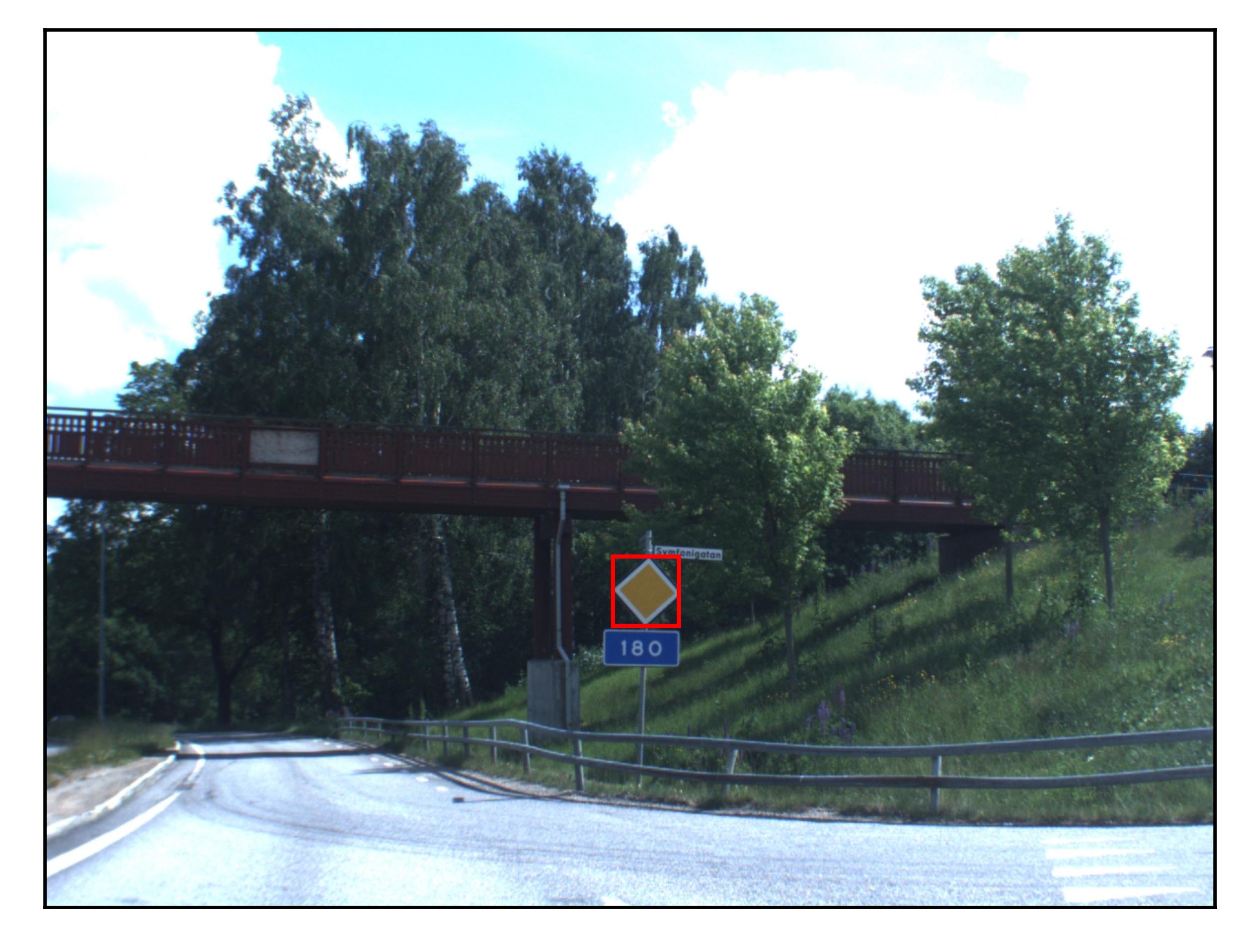
Figure 1: An example from the STS dataset for traffic sign detection. The original image is of size $960\times 1,280\times 3$. The red bounding box of a small object treated as a positive instance only covers less than 1% of the original image.

We start with the construction of the feature vector. Specifically, for each original high–resolution image of $960\times 1,280$, a pretrained VGG16 model is applied (Simonyan and Zisserman, 2014). This results in a feature map of size $30\times 40\times 512$. This feature map can be viewed as a new “image” with resolution $30\times 40$ and a total of 512 channels. In this regard, each pixel in this feature map can be treated as one sample with a feature vector of $p=512$ dimensions. This leads to the feature vectors as $\{\mathbb{X}_{i,k_{1},k_{2}}\in\mathbb{R}^{p}:1\leq k_{1}\leq 30,1\leq k_{2}\leq 40\}$. Therefore, a total of $30\times 40=1,200$ samples can be obtained for each image. Because a total of 1,970 images are involved in the whole dataset, the total sample size in this study is then $N=1,970\times 1,200=2,364,000$. Next, for each $\mathbb{X}_{i,k_{1}k_{2}}$, we generate a binary response $\mathbb{Y}_{i,k_{1},k_{2}}$ based on whether a traffic sign is involved in the pixel location. This leads to labels as $\{\mathbb{Y}_{i,k_{1},k_{2}}\in\mathbb{R}:1\leq k_{1}\leq 30,1\leq k_{2}\leq 40\}$. The number of positive instances accounts for only 0.225% of the total sample, which is expected because the region containing traffic signs in a high–resolution image is extremely small. Once the data are well prepared, the training data are randomly split into two parts. In the first part, the labels of the samples are treated as if they were missing. The second part is treated as if the labels of the samples were observed. Thereafter, the MEM algorithm can be applied to the training data. For a comprehensive evaluation, six different labeled percentages (i.e., $m/(N+m)\times 100$%) are evaluated. They are, respectively, 0%, 5%, 25%, 50%, 75% and 100%. For a reliable evaluation, the experiment is randomly replicated for $D=20$ times.

To gauge the finite sample performance of the proposed method, three different measures are used. The first measure is area under the curve (AUC) (Ling et al., 2003). Consider the $i^{*}$th image ($1\leq i^{*}\leq N^{*}$) in the test data, where $N^{*}=394$ denotes the number of images for testing. For a given pixel $(k_{1},k_{2})$ and one particular estimator $\widehat{\theta}$ obtained from the train data, we then estimate the response probability of $\widehat{\pi}_{i^{*},k_{1},k_{2}}=f_{\widehat{\theta}}(\mathbb{X}_{i^{*},k_{1},k_{2}})^{-1}\alpha\phi_{\widehat{\mu}_{1},\widehat{\Sigma}_{1}}(\mathbb{X}_{i^{*},k_{1},k_{2}})$. Accordingly, the AUC measure can be computed at the image level and denoted by ${\rm AUC}_{i^{*}}$. The image-level AUC is then averaged across different images, and denoted by AUC${}^{*}=N^{*-1}\sum_{i^{*}}{\rm AUC}_{i^{*}}$. The replicated AUC^∗ values are averaged across the random replications and are denoted as $\overline{\rm AUC}$. The second measure is the number of false positives. For a given random replication and the $i^{*}$th image, we can predict $\widehat{\mathbb{Y}}_{i^{*},k_{1},k_{2}}=I\big{(}\widehat{\pi}_{i^{*},k_{1},k_{2}}>c_{i^{*}}\big{)}$, where $c_{i}^{*}$ is the largest threshold value so that all positive instances can be correctly captured. However, the price is inevitably paid by mistakenly predicting some negative samples as positives. We define the number of false positives for the $i^{*}$th image in the test data as ${\rm FP}_{i^{*}}=\sum_{k_{1},k_{2}}I\big{(}\widehat{\mathbb{Y}}_{i^{*},k_{1},k_{2}}=1\big{)}I\big{(}\mathbb{Y}_{i^{*},k_{1},k_{2}}=0\big{)}$. Its median value is then computed as ${\rm FP^{*}}$. Then its overall mean across different random replications is denoted by $\overline{\rm FP}$. The third measure is the number of iterations used for the numerical convergence and denoted as $N_{\rm iter}^{*}$. The averaged $N_{\rm iter}^{*}$ values across the random replications are computed and denoted as $\overline{N_{\rm iter}}$ as an overall measure. The prediction results are presented in Figure 2.

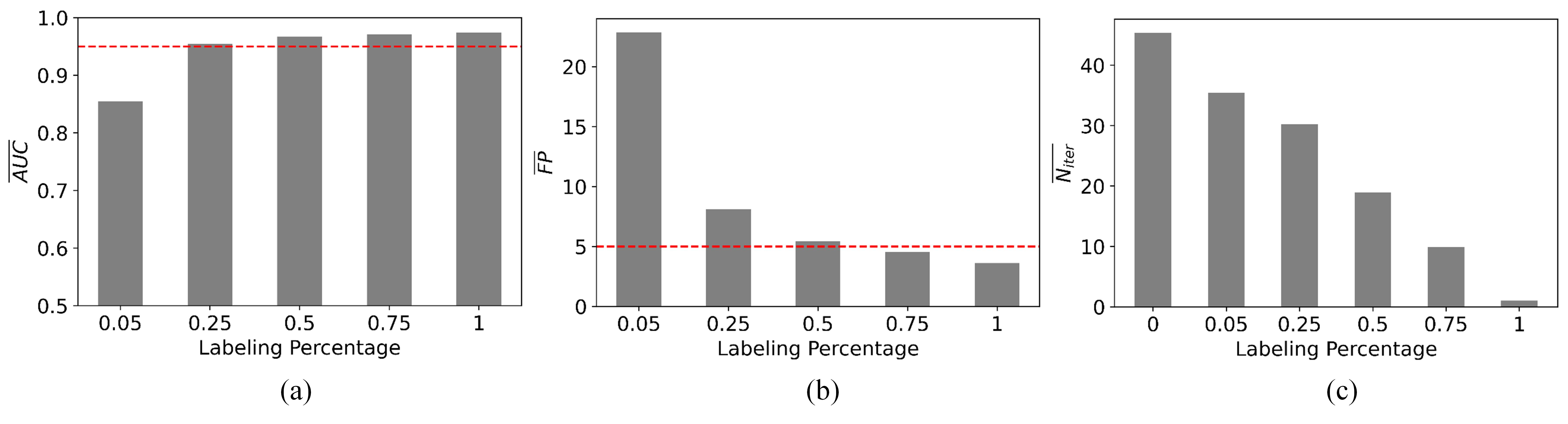
Figure 2: Detailed prediction results obtained from the test data. The left panel demonstrates the $\overline{\rm AUC}$ results. The red dashed line corresponds to $\overline{\rm AUC}=0.95$. The middle panel presents the $\overline{\rm FP}$ results. The red dashed line corresponds to $\overline{\rm FP}=5$. The right panel shows the $\overline{N_{\rm iter}}$ results.

We find that the $\overline{\rm AUC}$ value is 0.5235 and $\overline{\rm FP}$ value is 1,098.85 when the labeling percentage is 0%. These are totally not comparable with the other cases and thus not presented in Figure 2. This suggests that the prediction performance of the standard EM algorithm for a GMM with rare events could be extremely poor. However, the performance can be significantly improved if the data are partially labeled. A quick glance at Figure 2 suggests that cases with labeling percentages larger than 25% perform well in terms of $\overline{\rm AUC}$ values. For example, consider the case with a labeling percentage being 25%. The $\overline{\rm AUC}$ value becomes 0.9547, which is slightly worse than the 0.9711 for the fully labeled case. Similar observations are also observed for other performance measures (i.e., $\overline{\rm FP}$ and $\overline{N_{\rm iter}}$). Specifically, when the labeling percentage is 50%, the $\overline{\rm FP}$ value becomes 5.45, which is slightly worse than the 3.63 value obtained in the fully labeled case. Meanwhile, the $\overline{N_{\rm iter}}$ value becomes 18.95, which performs much better than the 45.35 value obtained in the fully unlabeled case.

5 Concluding Remarks

In this study, we focus on a problem related to the analysis of rare events data. Statistical analysis of rare events data differs significantly from that of regular data, and considerable progress has been made in the field concerning rare events data analysis (Nguyen et al., 2012; Wang, 2020; Wang et al., 2021; Triguero et al., 2015, 2016; Duan et al., 2020). However, the existing methods often suffer from one common limitation. That is the dataset must be fully labeled. Thus, the problem of unsupervised or semi-supervised learning remains open for discussion. In our first attempt, we investigate here a GMM with rare events. The EM algorithm has been commonly used to estimate GMM (Wu, 1983; Xu and Jordan, 1996). Consequently, we study the theoretical properties of the standard EM algorithm for a GMM with rare events. To this end, we formulate an EM algorithm for a GMM with rare events as an iterated algorithm governed by a contraction operator. Our results suggest that the numerical convergence rate of the standard EM algorithm is extremely slow. To address this, we develop an MEM algorithm. We theoretically demonstrate that the numerical convergence rate of this algorithm is significantly higher than that of a standard EM algorithm if the labeled percentage is carefully designed.

To conclude this work, we would like to discuss some intriguing avenues for future research. Firstly, in this study, our focus was solely on the GMM as a parametric model. However, given the widespread use of various learning methods, such as deep neural networks, it would be of great interest to explore more complex and general models for rare events data in future research projects. Secondly, although we examined a GMM with only two underlying classes, our theoretical results can be extended to scenarios involving multiple classes with minimal modifications. Nevertheless, contemporary classification problems often involve a growing number of classes. Exploring how to extend our theoretical findings to address such challenging cases would be an intriguing direction for future exploration. Lastly, most existing literature on semi-supervised learning, including this study, has assumed that both positive and negative instances in previously labeled samples are accurately annotated. However, in situations where positive instances are rare, we often encounter cases where only the labels for positive instances are practically available, whereas the labels for negative instances are too numerous to be analytically provided. This presents an interesting scenario where only positive instances are practically labeled. Exploring solutions for this problem is another fascinating topic worthy of investigation.

Acknowledgments

Jing Zhou’s research is supported in part by the National Natural Science Foundation of China (No.72171226, 11971504) and the National Statistical Science Research Project (No.2023LD008). Hansheng Wang’s research is partially supported by the National Natural Science Foundation of China (No.12271012)

References

- Amaro et al. (2018) Rommie E Amaro, Jerome Baudry, John Chodera, Özlem Demir, J Andrew McCammon, Yinglong Miao, and Jeremy C Smith. Ensemble docking in drug discovery. Biophysical Journal, 114(10):2271–2278, 2018.
- Bagui and Li (2021) Sikha Bagui and Kunqi Li. Resampling imbalanced data for network intrusion detection datasets. Journal of Big Data, 8(1):1–41, 2021.
- Bao et al. (2016) Lei Bao, Cao Juan, Jintao Li, and Yongdong Zhang. Boosted near-miss under-sampling on svm ensembles for concept detection in large-scale imbalanced datasets. Neurocomputing, 172:198–206, 2016.
- Biernacki et al. (2003) Christophe Biernacki, Gilles Celeux, and Gérard Govaert. Choosing starting values for the em algorithm for getting the highest likelihood in multivariate gaussian mixture models. Computational Statistics & Data Analysis, 41(3-4):561–575, 2003.
- Boldea and Magnus (2009) Otilia Boldea and Jan R Magnus. Maximum likelihood estimation of the multivariate normal mixture model. Journal of the American Statistical Association, 104(488):1539–1549, 2009.
- Chandola et al. (2009) Varun Chandola, Arindam Banerjee, and Vipin Kumar. Anomaly detection: A survey. ACM Computing Surveys (CSUR), 41(3):1–58, 2009.
- Daskalakis et al. (2017) Constantinos Daskalakis, Christos Tzamos, and Manolis Zampetakis. Ten steps of em suffice for mixtures of two gaussians. In Conference on Learning Theory, pages 704–710. PMLR, 2017.
- Dempster et al. (1977) Arthur P Dempster, Nan M Laird, and Donald B Rubin. Maximum likelihood from incomplete data via the em algorithm. Journal of the Royal Statistical Society: Series B (Methodological), 39(1):1–22, 1977.
- Duan et al. (2020) Moming Duan, Duo Liu, Xianzhang Chen, Renping Liu, Yujuan Tan, and Liang Liang. Self-balancing federated learning with global imbalanced data in mobile systems. IEEE Transactions on Parallel and Distributed Systems, 32(1):59–71, 2020.
- Feng et al. (2013) Changyong Feng, Hongyue Wang, Yu Han, Yinglin Xia, and Xin M Tu. The mean value theorem and taylor’s expansion in statistics. The American Statistician, 67(4):245–248, 2013.
- Gu et al. (2019) Yu Gu, Xiaoqi Lu, Baohua Zhang, Ying Zhao, Dahua Yu, Lixin Gao, Guimei Cui, Liang Wu, and Tao Zhou. Automatic lung nodule detection using multi-scale dot nodule-enhancement filter and weighted support vector machines in chest computed tomography. PLoS One, 14(1):e0210551, 2019.
- Gulati et al. (2013) Nikhil Gulati, Rachel Greenstadt, Kapil R Dandekar, and John M Walsh. Gmm based semi-supervised learning for channel-based authentication scheme. In 2013 IEEE 78th Vehicular Technology Conference (VTC Fall), pages 1–6. IEEE, 2013.
- Heimann et al. (2009) Tobias Heimann, Bram Van Ginneken, Martin A Styner, Yulia Arzhaeva, Volker Aurich, Christian Bauer, Andreas Beck, Christoph Becker, Reinhard Beichel, György Bekes, et al. Comparison and evaluation of methods for liver segmentation from ct datasets. IEEE transactions on medical imaging, 28(8):1251–1265, 2009.
- Korkmaz (2020) Selcuk Korkmaz. Deep learning-based imbalanced data classification for drug discovery. Journal of chemical information and modeling, 60(9):4180–4190, 2020.
- Kotz and Nadarajah (2000) Samuel Kotz and Saralees Nadarajah. Extreme value distributions: theory and applications. world scientific, 2000.
- Krivko (2010) M. Krivko. A hybrid model for plastic card fraud detection systems. Expert Systems with Applications, 37(8):6070–6076, 2010. ISSN 0957-4174. doi: https://doi.org/10.1016/j.eswa.2010.02.119. URL https://www.sciencedirect.com/science/article/pii/S0957417410001582.
- Larsson and Felsberg (2011) Fredrik Larsson and Michael Felsberg. Using fourier descriptors and spatial models for traffic sign recognition. In Anders Heyden and Fredrik Kahl, editors, Image Analysis, pages 238–249, Berlin, Heidelberg, 2011. Springer Berlin Heidelberg. ISBN 978-3-642-21227-7.
- Larsson et al. (2011) Fredrik Larsson, Michael Felsberg, and P-E Forssen. Correlating fourier descriptors of local patches for road sign recognition. IET Computer Vision, 5(4):244–254, 2011.
- Li et al. (2023) Xuetong Li, Xuening Zhu, and Hansheng Wang. Distributed logistic regression for massive data with rare events. arXiv preprint arXiv:2304.02269, 2023.
- Ling et al. (2003) Charles X Ling, Jin Huang, Harry Zhang, et al. Auc: a statistically consistent and more discriminating measure than accuracy. In Ijcai, volume 3, pages 519–524, 2003.
- Liu et al. (2009) Ya-Qin Liu, Cheng Wang, and Lu Zhang. Decision tree based predictive models for breast cancer survivability on imbalanced data. In 2009 3rd international conference on bioinformatics and biomedical engineering, pages 1–4. IEEE, 2009.
- Ma et al. (2000) Jinwen Ma, Lei Xu, and Michael I. Jordan. Asymptotic convergence rate of the em algorithm for gaussian mixtures. Neural Computation, 12(12):2881–2907, 2000. doi: 10.1162/089976600300014764.
- Magnus and Neudecker (2019) Jan R Magnus and Heinz Neudecker. Matrix differential calculus with applications in statistics and econometrics. John Wiley & Sons, 2019.
- Magnus (1988) JR Magnus. Linear structures. Griffin’s statistical monographs and courses, (42), 1988.
- Mansoor et al. (2015) Awais Mansoor, Ulas Bagci, Brent Foster, Ziyue Xu, Georgios Z Papadakis, Les R Folio, Jayaram K Udupa, and Daniel J Mollura. Segmentation and image analysis of abnormal lungs at ct: current approaches, challenges, and future trends. Radiographics, 35(4):1056–1076, 2015.
- McLachlan and Basford (1988) Geoffrey J McLachlan and Kaye E Basford. Mixture models: Inference and applications to clustering, volume 38. M. Dekker New York, 1988.
- McLachlan et al. (2019) Geoffrey J McLachlan, Sharon X Lee, and Suren I Rathnayake. Finite mixture models. Annual review of statistics and its application, 6:355–378, 2019.
- McNicholas (2016) Paul D McNicholas. Mixture model-based classification. Chapman and Hall/CRC, 2016.
- Mohammed et al. (2020) Roweida Mohammed, Jumanah Rawashdeh, and Malak Abdullah. Machine learning with oversampling and undersampling techniques: overview study and experimental results. In 2020 11th international conference on information and communication systems (ICICS), pages 243–248. IEEE, 2020.
- Naim and Gildea (2012) Iftekhar Naim and Daniel Gildea. Convergence of the em algorithm for gaussian mixtures with unbalanced mixing coefficients. In International Conference on Machine Learning, 2012.
- Nguyen et al. (2012) Hien M Nguyen, Eric W Cooper, and Katsuari Kamei. A comparative study on sampling techniques for handling class imbalance in streaming data. In The 6th International Conference on Soft Computing and Intelligent Systems, and The 13th International Symposium on Advanced Intelligence Systems, pages 1762–1767. IEEE, 2012.
- Pimentel et al. (2014) Marco AF Pimentel, David A Clifton, Lei Clifton, and Lionel Tarassenko. A review of novelty detection. Signal Processing, 99:215–249, 2014.
- Polat (2022) Hasan Polat. A modified deeplabv3+ based semantic segmentation of chest computed tomography images for covid-19 lung infections. International Journal of Imaging Systems and Technology, 32(5):1481–1495, 2022.
- Pozo et al. (2021) Rubén Fernández Pozo, Ana Belén Rodríguez González, Mark Richard Wilby, Juan José Vinagre Díaz, and Miguel Viana Matesanz. Prediction of on-street parking level of service based on random undersampling decision trees. IEEE Transactions on Intelligent Transportation Systems, 23(7):8327–8336, 2021.
- Qian et al. (2008) Feng Qian, Guang-min Hu, and Xing-miao Yao. Semi-supervised internet network traffic classification using a gaussian mixture model. AEU-International Journal of Electronics and Communications, 62(7):557–564, 2008.
- Royden and Fitzpatrick (1988) Halsey Lawrence Royden and Patrick Fitzpatrick. Real analysis, volume 32. Macmillan New York, 1988.
- Sanz et al. (2015) José Antonio Sanz, Dario Bernardo, Francisco Herrera, Humberto Bustince, and Hani Hagras. A compact evolutionary interval-valued fuzzy rule-based classification system for the modeling and prediction of real-world financial applications with imbalanced data. IEEE Transactions on Fuzzy Systems, 23(4):973–990, 2015. doi: 10.1109/TFUZZ.2014.2336263.
- Setio et al. (2017) Arnaud Arindra Adiyoso Setio, Alberto Traverso, Thomas De Bel, Moira SN Berens, Cas Van Den Bogaard, Piergiorgio Cerello, Hao Chen, Qi Dou, Maria Evelina Fantacci, Bram Geurts, et al. Validation, comparison, and combination of algorithms for automatic detection of pulmonary nodules in computed tomography images: the luna16 challenge. Medical Image Analysis, 42:1–13, 2017.
- Sigholm and Raciti (2012) Johan Sigholm and Massimiliano Raciti. Best-effort data leakage prevention in inter-organizational tactical manets. In MILCOM 2012-2012 IEEE Military Communications Conference, pages 1–7. IEEE, 2012.
- Simonyan and Zisserman (2014) Karen Simonyan and Andrew Zisserman. Very deep convolutional networks for large-scale image recognition. arXiv preprint arXiv:1409.1556, 2014.
- Spelmen and Porkodi (2018) Vimalraj S Spelmen and R Porkodi. A review on handling imbalanced data. In 2018 international conference on current trends towards converging technologies (ICCTCT), pages 1–11. IEEE, 2018.
- Tang et al. (2009) Yuchun Tang, Yan-Qing Zhang, Nitesh V. Chawla, and Sven Krasser. Svms modeling for highly imbalanced classification. IEEE Transactions on Systems, Man, and Cybernetics, Part B (Cybernetics), 39(1):281–288, 2009. doi: 10.1109/TSMCB.2008.2002909.
- Triguero et al. (2015) Isaac Triguero, Mikel Galar, Sarah Vluymans, Chris Cornelis, Humberto Bustince, Francisco Herrera, and Yvan Saeys. Evolutionary undersampling for imbalanced big data classification. In 2015 IEEE Congress on Evolutionary Computation (CEC), pages 715–722. IEEE, 2015.
- Triguero et al. (2016) Isaac Triguero, Mikel Galar, D Merino, Jesus Maillo, Humberto Bustince, and Francisco Herrera. Evolutionary undersampling for extremely imbalanced big data classification under apache spark. In 2016 IEEE congress on evolutionary computation (CEC), pages 640–647. IEEE, 2016.
- Wang (2020) HaiYing Wang. Logistic regression for massive data with rare events. In International Conference on Machine Learning, pages 9829–9836. PMLR, 2020.
- Wang et al. (2021) HaiYing Wang, Aonan Zhang, and Chong Wang. Nonuniform negative sampling and log odds correction with rare events data. Advances in Neural Information Processing Systems, 34:19847–19859, 2021.
- Wu (1983) CF Jeff Wu. On the convergence properties of the em algorithm. The Annals of Statistics, pages 95–103, 1983.
- Xu et al. (2016) Ji Xu, Daniel J Hsu, and Arian Maleki. Global analysis of expectation maximization for mixtures of two gaussians. Advances in Neural Information Processing Systems, 29, 2016.
- Xu and Jordan (1996) Lei Xu and Michael I Jordan. On convergence properties of the em algorithm for gaussian mixtures. Neural Computation, 8(1):129–151, 1996.