TokenUnify: Scalable Autoregressive Visual Pre-training with Mixture Token Prediction

Abstract

Autoregressive next-token prediction is a standard pretraining method for large-scale language models, but its application to vision tasks is hindered by the non-sequential nature of image data, leading to cumulative errors. Most vision models employ masked autoencoder (MAE) based pretraining, which faces scalability issues. To address these challenges, we introduce TokenUnify, a novel pretraining method that integrates random token prediction, next-token prediction, and next-all token prediction. We provide theoretical evidence demonstrating that TokenUnify mitigates cumulative errors in visual autoregression. Cooperated with TokenUnify, we have assembled a large-scale electron microscopy (EM) image dataset with ultra-high resolution, ideal for creating spatially correlated long sequences. This dataset includes over 120 million annotated voxels, making it the largest neuron segmentation dataset to date and providing a unified benchmark for experimental validation. Leveraging the Mamba network inherently suited for long-sequence modeling on this dataset, TokenUnify not only reduces the computational complexity but also leads to a significant 45% improvement in segmentation performance on downstream EM neuron segmentation tasks compared to existing methods. Furthermore, TokenUnify demonstrates superior scalability over MAE and traditional autoregressive methods, effectively bridging the gap between pretraining strategies for language and vision models. Code is available at https://github.com/ydchen0806/TokenUnify.

1 Introduction

Large language models (LLMs) can be scaled up to trillions of parameters through pretraining achiam2023gpt ; touvron2023llama ; touvron2023llama2 , primarily owing to high-quality data and effective autoregressive models. These models benefit from strong scaling laws because the structured and sequential nature of text data allows unification into a single next-token prediction task. However, when extending to multimodal tasks such as Unified IO lu2023unified and Qwen VL Qwen-VL , these models often fail to achieve state-of-the-art performance on fine-grained image tasks. This is due to an over-reliance on the capabilities of LLMs and a lack of robust pretraining strategies for visual data, resulting in weak visual representation capabilities.

Unlike language, the complexity of visual signals has led to diverse approaches in visual pretraining. Contrastive learning methods like DINO v2 oquab2023dinov2 excel in fine-grained representation, while masked reconstruction methods such as MAE he2022masked ; chen2023self offer good scalability and zero-shot classification abilities. However, these methods exhibit poor scaling laws, where increasing model size does not yield expected performance gains singh2023effectiveness (see Section A in the appendix). To achieve scaling laws similar to language models, approaches like AIM el2024scalable and LVM bai2023sequential have introduced autoregressive tasks into the visual domain, showing promising scaling properties. However, image sequence disorder and error accumulation in autoregressive tasks often degrade performance in smaller models bachmann2024pitfalls . Additionally, the computational burden of long-sequence images makes researching image autoregressive tasks particularly challenging. We summarize the challenges of visual autoregressive tasks as follows: 1) How to reduce error accumulation in visual autoregression to achieve stronger scaling laws? 2) How to develop more efficient computational methods to handle massive image data? 3) How to construct spatially correlated long-sequence relationships in images?

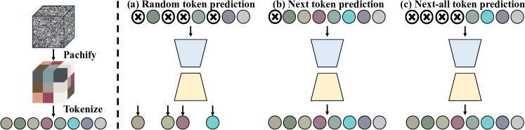
Figure 1: TokenUnify prediction paradigms divide the 3D EM image into non-overlapping patches, which are tokenized into a sequence. Three tasks are performed for rich 3D image representations: (a) random token prediction, (b) next token prediction, and (c) next-all token prediction.

This paper aims to tackle the above three critical challenges. 1) To tackle the issue of cumulative errors in visual autoregression, we propose TokenUnify, a novel mixed token prediction paradigm. TokenUnify integrates next-token prediction, next-all token prediction, and random token prediction (as illustrated in Fig. 1), leveraging global information to overcome the limitations of local receptive fields. We theoretically demonstrate that this mixed approach reduces cumulative errors while maintaining favorable scaling laws. 2) To alleviate computational burdens, we introduce the Mamba architecture, which reduces the computational complexity of autoregressive tasks from quadratic (as in Transformers) to linear. Detailed comparisons of the scaling properties between Mamba and Transformer architectures reveal that Mamba achieves superior performance and efficiency in large-scale autoregressive visual models. 3) To construct spatially correlated long-sequence relationships, we have collected large-scale, ultra-high-resolution 3D electron microscopy (EM) images of mouse brain slices. The ultra-high resolution allows for thousands of continuous image tokens, ensuring robust spatial continuity. We have fully annotated six different functional regions within the mouse brain, totaling 120 million pixels, resulting in the largest manually annotated neuron dataset to date. This comprehensive dataset also serves as a unified benchmark for evaluating experimental performance .

Pretraining with TokenUnify led to a 45% improvement in performance on subsequent EM neuron segmentation tasks. The mixed training paradigm of TokenUnify outperformed MAE he2022masked by 21% in pretraining performance, even with fewer parameters. Furthermore, TokenUnify demonstrated superior scaling properties of autoregressive models, offering a promising approach for pretraining large-scale visual models.

Our contributions can be summarized as follows:

1. We introduce a novel pre-training paradigm, TokenUnify, which models visual pre-training tasks from multiple perspectives at the token level. This ensures sublinear growth of the scaling law while demonstrating superior fine-grained feature extraction capabilities compared to MAE in smaller model pre-training. We also provide a theoretical explanation for this phenomenon.

2. We achieve a 45% performance improvement on the neuron segmentation task and, for the first time, validate the Mamba model with billion-level parameters on visual tasks, demonstrating the effectiveness and efficiency of TokenUnify in long-sequence visual autoregression.

3. We provide a large-scale biological image dataset with 120 million annotated pixels, offering a long-sequence image dataset to validate the potential of autoregressive methods.

2 Related work

Recent advances in large language models (LLMs) have unified various NLP tasks under a single architecture, formulating them as generation tasks. This architecture can be categorized into BERT-like devlin2018bert ; xia2020bert ; lee2020biobert ; song23c_interspeech and GPT-like brown2020language ; radford2019language ; li2024exploring ; zhou2023thread models. The latter, decoder-only autoregressive structure, has been shown to be more effective, as validated by products like ChatGPT. Subsequent works have built upon GPT, introducing techniques like RMSNorm zhang2019root , SwiGLU, and RoPE to ensure efficient and stable training. The LLaMA series touvron2023llama ; touvron2023llama2 has improved training efficiency, while the Qwen series Qwen-VL ; bai2023qwen ; xiang2024research has focused on data cleaning and filtering for Chinese language models. Currently, LLMs have surpassed human-level performance in many text processing tasks achiam2023gpt .

In multi-modal tasks, the CLIP radford2021learning and BLIP series li2022blip ; li2023blip ; dai2024instructblip have pioneered contrastive learning on image-text pairs, achieving remarkable zero-shot classification and generalization capabilities. Further works zhang2023large ; chen2023generative ; wang2022medclip ; zhou2024visual have applied multi-modal models to specific domains. By processing arbitrary modalities into a unified token format lu2023unified ; wang2023distributed ; chen2024subject , these models can generate outputs in any modality. However, there is still room for improvement in fine-grained visual tasks, and training large vision models remains an open problem.

Self-supervised pre-training has been a cornerstone for enhancing model representation capabilities. Approaches based on contrastive learning for representation extraction chen2024learning ; zbontar2021barlow ; he2020momentum ; li2021consistent and masked reconstruction methods he2022masked ; chen2023self ; li2023mage ; ding2022unsupervised ; chen2024bridging ; chen2023point have shown promise. However, current vision models have not exhibited the same sublinear scaling laws as language models. To address this issue, some tasks have adopted autoregressive pre-training paradigms similar to those used in language models chen2020generative ; bai2023sequential ; el2024scalable , though the training costs remain a significant concern. In this paper, we explore the potential of long visual token autoregressive pre-training and introduce a collaborative training scheme for long token prediction. Our approach aims to balance the scaling laws and training costs, demonstrating improvements in fine-grained visual tasks.

3 Method

3.1 Overview

Our theoretical contributions include proving the parameter independence of MAE performance (see Section A), establishing the strong correlation between autoregressive model performance and parameter count (see Section B), and demonstrating the advantages of next-all token prediction from both intuitive (see Section C.1) and theoretical perspectives (see Section C.2).

Our experimental framework comprises two stages: pre-training and fine-tuning. During the pre-training stage, we leverage only the unlabeled raw data $\mathcal{X}$ to learn a generic visual representation $f_{\theta_{1}}(\cdot)$, parameterized by $\theta_{1}$. We employ a mixed token prediction strategy to capture both local and global dependencies in the data (see Section 3.2). Additionally, we utilize Mamba for efficient modeling of long sequences in autoregressive tasks, enhancing computational efficiency (see Section 3.3).

In the fine-tuning stage, we use both the raw data $\mathcal{X}$ and the corresponding labels $\mathcal{Y}$ to adapt the pre-trained representation to specific downstream tasks. Let $g_{\theta_{2}}(\cdot)$ be the task-specific model, parameterized by $\theta_{2}$. We initialize $\theta_{2}$ with the pre-trained weights $\theta_{1}$ and optimize the task-specific objective. Further details are provided in Sections 3.4 and F.3.

To illustrate the application of our framework, consider the modeling of EM images. Given a total of $T$ EM images $\mathcal{X}={\mathbf{X}^{(1)},\ldots,\mathbf{X}^{(T)}}$, where each $\mathbf{X}^{(t)}\in\mathbb{R}^{D\times H\times W}$ represents a 3D image with depth $D$, height $H$, and width $W$, we aim to learn a meaningful representation of this high-dimensional, long-sequence visual data by leveraging its inherent spatial structure and continuity. To achieve this, we partition each large 3D image $\mathbf{X}$ into smaller patches $\mathbf{x}\in\mathbb{R}^{D^{\prime}\times H^{\prime}\times W^{\prime}}$.

3.2 Mixed-mode autoregressive modeling

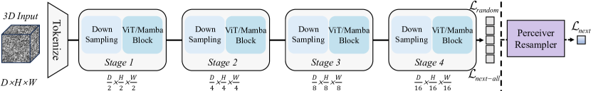
Figure 2: illustrates the main pretraining workflow of TokenUnify. The image $\mathbf{X}$ is fed into the Tokenizer, transforming it into a long sequence of tokens $\mathbf{x}_{i}|_{i=1}^{K}$. The predictions for the random token, next token, and next-all token are performed sequentially. The Perceiver Resampler is employed to convert varying-size large feature maps into a few visual tokens (see Section 3.2).

We theoretically demonstrate the effectiveness of MAE he2022masked on smaller models, the scaling advantages of next token prediction, and the ability of next-all token prediction to mitigate cumulative errors in autoregressive models. Based on these insights, we propose a hybrid training paradigm that aims to combine the strengths of these three methods, as shown in Fig. 2.

Given an image $\mathbf{X}$, we first divide it into a sequence of $K$ non-overlapping patches $\{\mathbf{x}_{1},\ldots,\mathbf{x}_{K}\}$. Standard autoregressive modeling typically adopts a fixed left-to-right factorization:

$$p(\mathbf{x})=\prod\nolimits_{i=1}^{K}p(\mathbf{x}_{i}\mid\mathbf{x}_{<i}),$$ (1)

where $\mathbf{x}_{<i}$ denotes all patches preceding $\mathbf{x}_{i}$.

We introduce TokenUnify, a mixed-mode autoregressive modeling approach designed to enhance existing autoregressive image modeling techniques chen2020generative ; bai2023sequential . TokenUnify combines three distinct prediction tasks: random token prediction, next token prediction, and next-all token prediction, instead of using the fixed factorization in Eq. 1.

Random Token Prediction.

Given the full patch sequence $\mathbf{x}_{1:K}$, we randomly mask out a subset of patches $\mathcal{M}\subset\{1,\ldots,K\}$ and train the model to predict the masked patches conditioned on the remaining context:

$$\mathcal{L}_{\text{random}}=-\sum\nolimits_{i\in\mathcal{M}}\log p(\mathbf{x}_{i}|\mathbf{x}_{\bar{\mathcal{M}}}),$$ (2)

where $\mathbf{x}_{\bar{\mathcal{M}}}=\{\mathbf{x}_{i}\mid i\notin\mathcal{M}\}$ denotes the unmasked patches.

Next Token Prediction.

We integrate the standard next token prediction loss into our task. In this setup, we use the Perceiver Resampler alayrac2022flamingo (see Section F.2) to convert the variable-sized feature maps generated by the Vision Encoder into a fixed number of visual tokens. This loss trains the model to predict the next patch $\mathbf{x}i$ given the preceding context $\mathbf{x}_{<i}$:

$$\mathcal{L}_{\text{next}}=-\sum\nolimits_{i=1}^{K}\log p(\mathbf{x}_{i}|\mathbf{x}_{<i}).$$ (3)

Next-All Token Prediction.

To encourage the model to capture longer-range dependencies, we extend the next token prediction to a next-all token prediction task. For each patch $\mathbf{x}_{i}$, the model is trained to predict not only $\mathbf{x}_{i}$ but also all the subsequent patches $\mathbf{x}_{i:K}$ in the sequence:

$$\mathcal{L}_{\text{next-all}}=-\sum\nolimits_{i=1}^{K}\sum\nolimits_{j=i}^{K}\log p(\mathbf{x}_{j}|\mathbf{x}_{<i}).$$ (4)

By alternating between these token prediction tasks every 100 epochs, we prevent the model from converging to a trivial solution and encourage it to learn meaningful representations from the input data. This alternating training strategy enables the model to capture both local and global dependencies within the patch sequence, thereby enhancing performance on downstream tasks. The workflow of TokenUnify is illustrated in Fig. 2.

3.3 Mamba ordering

While the aforementioned mix token prediction task improves sequence autoregressive modeling capabilities, it also introduces additional computational complexity for long sequences. Inspired by the Mamba strategy proposed by gu2023mamba , we introduce an enhanced approach to effectively model long sequences in volumetric EM images. Traditional sequence modeling methods often struggle with capturing long-range dependencies due to their rigid sequential nature. Our enhanced Mamba ordering strategy addresses this by incorporating a more sophisticated and flexible sequence modeling approach.

The fundamental idea behind Mamba ordering is to dynamically prioritize regions of the sequence based on contextual significance rather than adhering to a fixed order. This is achieved through an adaptive mechanism that evaluates the importance of different patches within the sequence and adjusts the processing order accordingly. By doing so, Mamba ordering enhances the model’s ability to capture intricate patterns and long-range dependencies more effectively.

Mathematically, let $\mathbf{x}=\{\mathbf{x}_{1},\mathbf{x}_{2},\ldots,\mathbf{x}_{K}\}$ represent the sequence of patches. Instead of processing these patches in a fixed order, we define a dynamic ordering function $\sigma:\{1,2,\ldots,K\}\rightarrow\{1,2,\ldots,K\}$ that determines the sequence in which patches are processed. The Mamba ordering objective can be formulated as:

$$\mathcal{L}_{\text{mamba}}=-\mathbb{E}_{\mathbf{x}\sim p_{\text{data}}}\left[\sum\nolimits_{i=1}^{K}\log p(\mathbf{x}_{\sigma(i)}|\mathbf{x}_{\sigma(<i)})\right],$$ (5)

where $\mathbf{x}_{\sigma(<i)}$ represents the context preceding the $i$-th patch in the dynamically determined order.

To optimize this objective, we introduce a context-aware attention mechanism that assesses the relevance of each patch with respect to the overall sequence. This mechanism outputs a relevance score for each patch, guiding the dynamic ordering function $\sigma$ to prioritize patches that are most informative for subsequent predictions. By iteratively updating the relevance scores and reordering the patches, Mamba ordering ensures that the model focuses on the most crucial aspects of the sequence at each step.

Consider the state-space model representation where the hidden state $\mathbf{h}(t)$ evolves dynamically based on the input $\mathbf{x}(t)$. The state-space equations are given by:

$$\mathbf{h}^{\prime}(t)=\mathbf{A}(t)\mathbf{h}(t)+\mathbf{B}(t)\mathbf{x}(t),\quad\mathbf{y}(t)=\mathbf{C}(t)\mathbf{h}(t),$$ (6)

where $\mathbf{A}(t)$, $\mathbf{B}(t)$, and $\mathbf{C}(t)$ are time-dependent matrices. Specifically, $\mathbf{B}(t)$ and $\mathbf{C}(t)$ are parameterized by the input $\mathbf{x}(t)$ as follows:

$$\mathbf{B}(t)=s_{B}(\mathbf{x}(t)),\quad\mathbf{C}(t)=s_{C}(\mathbf{x}(t)),\quad\mathbf{\Delta}(t)=\tau_{\Delta}(\text{Linear}(\mathbf{x}(t))),$$ (7)

where $s_{B}$, $s_{C}$, and $\tau_{\Delta}$ are functions that map the input to the respective parameters.

The benefits of our enhanced Mamba ordering are twofold. First, it mitigates error accumulation by allowing the model to refine its predictions based on a globally coherent understanding of the sequence. Second, it enhances the model’s capacity to capture long-range dependencies, as the dynamic ordering can adapt to the inherent structure and complexity of the data.

Empirical results demonstrate that our enhanced Mamba ordering significantly improves the performance of sequence modeling tasks in volumetric EM images, particularly for long sequences. By enabling a more adaptive and context-aware approach to sequence processing, our enhanced Mamba ordering represents a substantial advancement over traditional methods, offering a robust and scalable solution for high-dimensional visual data.

3.4 Finetuning and Segmentation

The segmentation network, denoted as $g_{seg}(\cdot)$, consists of an encoder $g_{e}(\cdot)$ and a decoder $g_{d}(\cdot)$:

$$g_{seg}(x;\theta_{s})=g_{d}(g_{e}(x)),\quad\theta_{s}=\{\theta_{e},\theta_{d}\},$$ (8)

where $\theta_{s}$ represents the parameters of the entire segmentation network, and $\theta_{e}$ and $\theta_{d}$ are the parameters of the encoder and decoder, respectively.

The encoder $g_{e}(\cdot)$ gradually downsamples the input volume and extracts high-level semantic features, while the decoder $g_{d}(\cdot)$ upsamples the encoded features back to the original resolution. Meanwhile, the output of each downsampling layer in the encoder is connected to the corresponding layer in the decoder via skip connections to fuse local and global multi-scale information. We adopt 3D ResUNet/ViT/Mamba as the backbone network, respectively.

The output of the segmentation network $\hat{y}=g_{seg}(x)\in\mathbb{R}^{C\times D\times H\times W}$ represents the predicted affinity map li2018contextual ; li2023deception , corresponding to the connectivity probability of each voxel in three directions. During training, the loss function for labeled samples is the mean squared error between the predicted and ground-truth affinity maps:

$$L_{seg}=\frac{1}{|D_{l}|}\sum\nolimits_{i=1}^{|D_{l}|}\left|\hat{y}_{i}-y_{i}\right|^{2}=\frac{1}{|D_{l}|}\sum\nolimits_{i=1}^{|D_{l}|}\left|g_{seg}(x_{i}^{l})-y_{i}\right|^{2}.$$ (9)

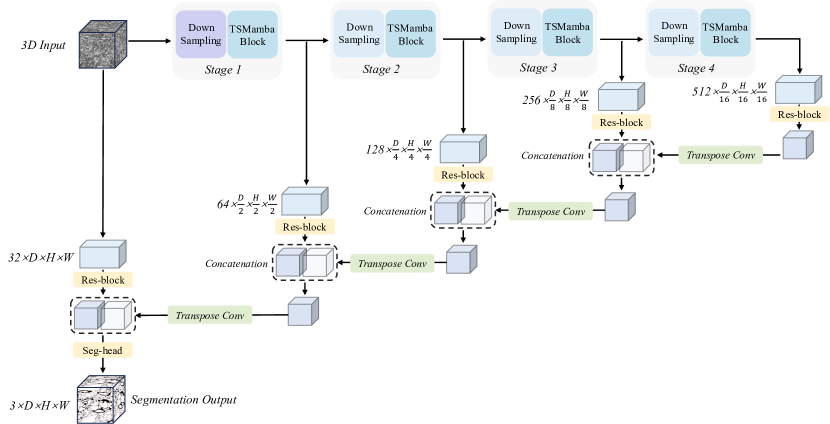
Figure 7: Segmentation pipeline.

During inference, for any new test sample $x_{t}$, forward propagation through $g_{seg}(x_{t})$ yields its predicted affinity map. This predicted affinity map is then post-processed using a seeded watershed algorithm and a structure-aware region agglomeration algorithm funke2018large ; beier2017multicut to obtain the final neuron instance segmentation. Detailed information on our segmentation process can be found in Section F.3, and the segmentation pipeline is illustrated in Fig. 7.

4 Dataset and Metrics

Dataset.

For the pretraining phase of TokenUnify, we collect a vast amount of publicly available unlabeled EM imaging data, from four large-scale electron microscopy (EM) datasets: Full Adult Fly Brain (FAFB) schlegel2021automatic , MitoEM wei2020mitoem , FIB-25 takemura2017connectome , and Kasthuri15 kasthuri2015saturated . These datasets cover a diverse range of organisms, including Drosophila, mouse, rat, and human samples, totaling over 1 TB. The details of the pretraining datasets can be found in Table 3. We sample from the datasets with equal probability and ensure that each brain region has an equal chance of being sampled, guaranteeing the diversity of the pretraining data.

For downstream fine-tuning and segmentation, we employ two datasets: a smaller dataset, AC3/4, and a larger dataset, MEC, for algorithm validation. The AC3/4 dataset kasthuri2015saturated consists of mouse somatosensory cortex datasets with 256 and 100 successive EM images (1024$\times$1024). We use the first 80 images of AC4 for fine-tuning, the last 20 images of AC4 for testing, and the first 100 images of AC3 for testing. Additionally, we have collected a large-scale electron microscopy dataset, MEC, by imaging the mouse somatosensory cortex, mouse medial entorhinal cortex, and mouse cerebral cortex, achieving a physical resolution of 8nm × 8nm × 40nm. We select 6 representative volumes from different neural regions, named wafer4/25/26/26-2/36/36-2, with each volume size reaching 125 × 1250 × 1250 voxels. We perform dense annotation on these selected wafer regions, with a total of over 1.2 billion annotated voxels. To validate the algorithm’s performance on a large-scale dataset, we use wafer25/26/26-2/36 for training, wafer4 for validation, and wafer36-2 for testing on the MEC dataset.

Metrics.

To evaluate the performance of neuron segmentation zhang2024research ; dang2024real , we employ two widely-used metrics: Variation of Information (VOI) nunez2013machine and Adjusted Rand Index (ARAND) arganda2015crowdsourcing . These metrics quantify the agreement between the predicted segmentation and the ground truth from different perspectives. Detailed descriptions of these metrics can be found in Section D.2.

Table 1: Quantitative comparison of segmentation results on Wafer4 and Wafer36-2 datasets. ‘Post.’ represents the post-processing algorithms. * denotes the MAE pretraining strategy he2022masked . † indicates our TokenUnify pretraining strategy. The best results are in bold and the second best results are in underlined.

Post.	Method	Wafer4				Wafer36-2				Param.
Waterz funke2018large		$VOI_{M}\downarrow$	$VOI_{S}\downarrow$	$VOI\downarrow$	$ARAND\downarrow$	$VOI_{M}\downarrow$	$VOI_{S}\downarrow$	$VOI\downarrow$	$ARAND\downarrow$	(M)
	Superhuman lee2017superhuman	0.3328	1.1258	1.4587	0.1736	0.1506	0.4588	0.6094	0.0836	1.478
	MALA funke2018large	0.5438	1.5027	2.0375	0.1115	0.3179	1.0664	1.3843	0.1570	84.02
	PEA huang2022learning	0.3381	0.9276	1.2658	0.0677	0.2787	0.4279	0.7066	0.1169	1.480
	UNETR hatamizadeh2022unetr	0.4504	1.6581	2.1085	0.2658	0.4478	0.5217	0.9696	0.2913	129.1
	EMmamba	0.4915	1.2924	1.7839	0.2052	0.2406	0.4189	0.6595	0.1231	28.30
	Superhuman*	0.2971	0.8965	1.1936	0.1108	0.1922	0.3819	0.5742	0.1025	1.478
	MALA*	0.7300	1.1694	1.8994	0.2295	0.5088	0.3945	0.9034	0.2574	84.02
	PEA*	0.2677	0.7866	1.0543	0.0454	0.2184	0.2971	0.5156	0.0906	1.480
	UNETR*	0.3127	0.8348	1.1475	0.0940	0.3982	0.3844	0.7825	0.1768	129.1
	EMmamba*	0.2120	1.0560	1.2680	0.0862	0.1449	0.4201	0.5650	0.0702	28.30
	EMmamba†	0.1953	0.7998	0.9951	0.0509	0.1262	0.3585	0.4848	0.0650	28.30
LMC beier2017multicut	Superhuman lee2017superhuman	0.1948	1.9697	2.1644	0.2453	0.0792	1.1618	1.2410	0.1319	1.478
	MALA funke2018large	0.3416	2.4129	2.7545	0.2567	0.1448	1.9603	2.1052	0.1977	84.02
	PEA huang2022learning	0.1705	1.5993	1.7698	0.1527	0.4719	1.1226	1.5945	0.1588	1.480
	UNETR hatamizadeh2022unetr	0.1791	3.1715	3.3506	0.6330	0.0949	1.3858	1.4807	0.1578	129.1
	EMmamba	0.1596	2.0580	2.2177	0.1973	0.0847	1.0351	1.1198	0.1253	28.30
	Superhuman*	0.2564	1.7823	2.0387	0.1812	0.0844	1.1317	1.2161	0.1289	1.478
	MALA*	0.2001	2.5742	2.7747	0.5622	0.3946	1.1652	1.5598	0.1543	84.02
	PEA*	0.4584	1.4873	1.9458	0.1254	0.4694	1.0217	1.4910	0.1413	1.480
	UNETR*	0.2389	1.8072	2.0461	0.1704	0.0985	1.1860	1.2845	0.1380	129.1
	EMmamba*	0.1319	1.8734	2.0054	0.1405	0.0726	1.0731	1.1457	0.1183	28.30
	EMmamba†	0.1418	1.5103	1.6521	0.0591	0.0827	1.0276	1.1103	0.1074	28.30

5 Experiment

Implementation Details.

In this work, we employ consistent training settings for both pretraining and fine-tuning tasks. The network architecture remains the same throughout the training and fine-tuning phases. During fine-tuning, we optimize the network using the AdamW optimizer loshchilov2018decoupled with $\beta_{1}=0.9$, $\beta_{2}=0.999$, a learning rate of 1e-6, and a batch size of 20 on an NVIDIA GTX 3090 (24GB) GPU. For pretraining, we use a batch size of 8 on an NVIDIA Tesla A40 (48G) GPU due to memory constraints.

We perform distributed training using 8 NVIDIA GTX 3090 GPUs for each segmentation task, running for a total of 1200 epochs. Similarly, we utilize 32 NVIDIA Tesla A40 GPUs for each pretraining task, running for 400 epochs. During the pretraining phase, the input consists solely of unlabeled data, whereas in the segmentation phase, both labeled and unlabeled data are used as input. The input block resolution for the network is set to $16\times 160\times 160$. To initialize the network for fine-tuning, we load the weights obtained from the pretraining phase, following the settings of previous works he2022masked .

To generate final segmentation results from the predicted affinities, we employ two representative post-processing methods: Waterz funke2018large and LMC beier2017multicut . Waterz iteratively merges fragments based on edge scores until a threshold is reached. We set the quantile to 50% and the threshold to 0.5 based on testing on MEC, and discretize scores into 256 bins. LMC formulates agglomeration as a minimum-cost multi-cut problem, extracting edge features as costs and solving with the Kernighan-Lin solver kernighan1970efficient . We maintain consistent post-processing settings across all experiments to ensure fair comparisons and conclusions about our method.

Table 2: Quantitative comparison of segmentation results on AC3/4 datasets. ‘w/o Pre.’ indicates models without pretraining, whereas ’w Pre.’ denotes models that utilize corresponding pretraining strategy. * denotes the MAE pretraining strategy he2022masked . † indicates our TokenUnify pretraining strategy. The best results are in bold and the second best results are in underlined.

Method	$VOI_{M}\downarrow$		$VOI_{S}\downarrow$		$VOI\downarrow$		$ARAND$		Param.
	w/o Pre.	w Pre.	w/o Pre.	w Pre.	w/o Pre.	w Pre.	w/o Pre.	w Pre.	(M)
Superhuman lee2017superhuman	0.4882	0.6162	0.6563	0.6308	1.1445	1.2470	0.1748	0.2505	1.478
MALA funke2018large	0.4571	0.3345	0.6767	0.7479	1.1338	1.0824	0.1664	0.1020	84.02
PEA huang2022learning	0.5522	0.3832	0.4980	0.6153	1.0502	0.9985	0.2093	0.1127	1.480
UNETR hatamizadeh2022unetr	0.7799	0.5339	0.7399	0.5573	1.5198	1.0912	0.2411	0.1796	129.1
EMmamba*	0.9378	0.3167	0.8629	0.7963	1.8007	1.1131	0.2840	0.1050	28.30
EMmamba†	0.9378	0.4479	0.8629	0.5439	1.8007	0.9918	0.2840	0.1366	28.30

Experimental Results on MEC Dataset.

As detailed in Section 4, we leverage a substantial dataset called MEC to assess the performance of our algorithm. For neuron segmentation tasks, we have implemented several representative methods, including Superhuman lee2017superhuman , MALA funke2018large , PEA huang2022learning , and UNETR hatamizadeh2022unetr . Our EMmamba model (see Section F.3) builds upon Segmamba xing2024segmamba and incorporates enhancements to various anisotropic structures to better accommodate the resolution of electron microscopy. All networks are trained using default open-source parameters. Additionally, we calculated the parameter count for all architectures.

Our experimental results are presented in Table 1. The upper part of the table shows the performance of these methods when directly applied to segmentation tasks. In contrast, the lower part of the table illustrates the performance of networks employing self-supervised pretraining. When comparing models with a similar number of parameters, our pretraining approach achieves approximately a 21% performance improvement over MAE and over a 45% improvement compared to direct training. Visualization results, as shown in Fig. 3, demonstrate that our approach significantly outperforms others in both neuron splitting and merging tasks.

Experimental Results on AC3/4 Datasets.

As noted in Section 4, we also evaluate the performance of all baseline methods on a smaller dataset. Compared to the MEC dataset, the total training scale (number of labeled pixels) of the AC3/4 dataset is only about 1/10 of that of MEC. In this low-data scenario, the Mamba architecture combined with TokenUnify pretraining achieves performance comparable to the latest SOTA PEA pertaining (as shown in Table 2). Additionally, it demonstrates approximately a 10% performance improvement over the MAE pretraining approach. This highlights the robustness of TokenUnify even with a limited number of fine-tuning samples.

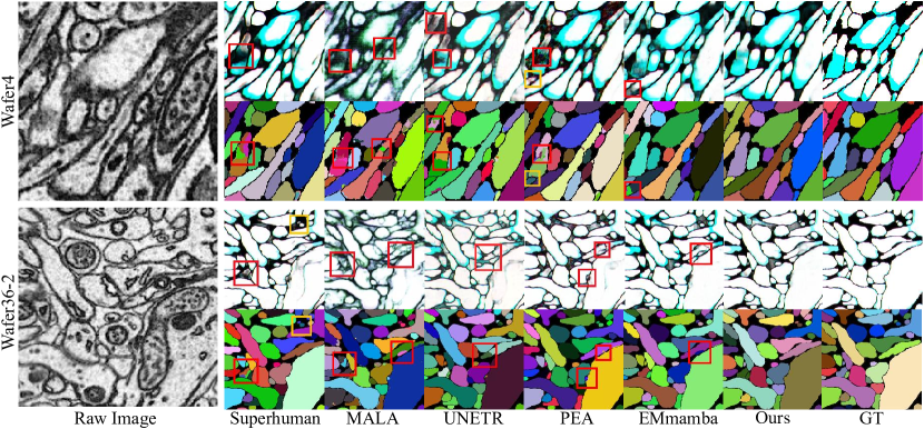
Figure 3: shows the visualization results for two slices from the MEC dataset: wafer 4 and wafer 36-2. The left side displays the EM raw images, while the right side presents the affinity and segmentation results. Red boxes indicate over-split regions, and orange boxes highlight over-merge regions.

Experimental Results on the Scaling Law.

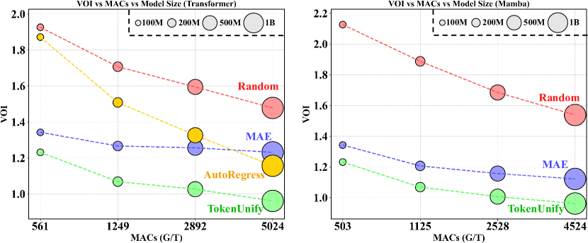
Figure 4: We evaluate the performance of models with 100M, 200M, 500M, and 1B parameters. Each model was trained for 100 epochs on the MEC and CREMI datasets.

We conducted a comprehensive evaluation of scaling laws for various initialization and training strategies: Random Initialization, MAE (Masked Autoencoder), Autoregressive, and our proposed TokenUnify method. By increasing the feature dimension and network depth, we scaled the model parameters to 100M, 200M, 500M, and 1B (detailed network structures are provided in Section F.3 and Table 5).

In our experiments, we tested input sizes of $16\times 160\times 160$. The Mamba architecture was trained on the MEC dataset, while the Transformer architecture was trained on the CREMI dataset funke2016miccai . Our experimental results are shown in Fig. 4.

Our findings indicate that, following pretraining on the same data, all methods except for the purely vision-based Autoregressive model with small parameter counts demonstrate performance gains. However, MAE quickly encounters scaling law limitations, hitting a performance bottleneck. In contrast, TokenUnify exhibits robust scaling properties, outperforming other pretraining methods at both small and large parameter scales. From a model architecture perspective, Mamba maintains segmentation performance while exhibiting a lower parameter count compared to the Transformer architecture. This validates the suitability of Mamba for long-sequence and autoregressive modeling tasks.

Abalation Study.

We conducted ablation studies on several components within our experimental setup. The experiments were divided into two main parts. First, we explored the mixed mechanisms of TokenUnify. We experimented with combinations of three different mixing mechanisms, ensuring that the total number of training epochs remained consistent. Table 6 presents the results of these experiments on the wafer4 neuron segmentation task (using a 28M EMmamba segmentation network). The results demonstrate that mixed training provides the most significant benefit for downstream tasks, with the combination of Random token and Next token being the next most effective.

Second, we performed ablation studies on the fine-tuning schemes. Under the default settings, we fine-tuned all parameters of the network. However, due to computational resource constraints, only a subset of parameters (or additional adapter parameters such as LoRA hu2022lora ) is often fine-tuned for larger models. Based on our network architecture (see Fig. 7), we divided the network into the Mamba part (for token sequence information extraction), the encoder part (for downsampling), and the decoder part (for convolutional upsampling). We fine-tuned only the corresponding subset of weights for each part. Our experimental results are shown in Table 7.

We found that in the TokenUnify modeling, using the sequence information priors extracted by Mamba significantly benefits downstream segmentation tasks. Combining the Mamba module with the encoder part yields even greater performance improvements, while fine-tuning only the encoder or decoder weights provides minimal gains. This suggests that in resource-constrained scenarios, fine-tuning only the sequence modeling parameters can be sufficient.

6 Social Impact and Future Work

The favorable scaling laws of TokenUnify present the opportunity to train a unified and generic visual feature extractor, which holds significant importance for visual tasks. A unified visual feature extractor can substantially reduce the cost of fine-tuning models for different visual tasks, thereby facilitating the application of visual technologies across various domains. We have currently validated the effectiveness of TokenUnify on long-sequence 3D medical images. Moving forward, we plan to further explore the performance of TokenUnify on natural images and other downstream tasks, thereby expanding its scope of application. Moreover, TokenUnify can be extended to multimodal domains such as image-text tasks chen2024bimcv ; liu2023t3d , demonstrating its utility in multimodal applications. We will also continue to investigate model lightweighting chen2023class ; chen2021multimodal and efficient fine-tuning strategies liu2023parameter ; li2024research . We believe that TokenUnify offers a promising approach for building large-scale, efficient visual pre-training models, contributing to advancements in the visual domain.

7 Conclusion

We propose TokenUnify, a novel autoregressive visual pre-training method that integrates random token prediction, next-token prediction, and next-all token prediction to effectively capture local and global dependencies in image data. We provide theoretical evidence demonstrating that TokenUnify mitigates cumulative errors in visual autoregression while maintaining favourable scaling laws. Furthermore, we collect a large-scale, ultra-high-resolution 3D electron microscopy dataset of mouse brain slices to serve as a unified benchmark for validating our approach. Pretraining with TokenUnify leads to a 45% improvement in performance on downstream neuron segmentation tasks compared to the baseline, showcasing the potential of our method in fine-grained visual tasks.

Appendix

Appendix A Why Does MAE Face Scaling Law Limitations?

Assumption 1.

Suppose the observations $y\in\mathbb{R}^{n}$ are generated by the linear model:

$$y=X\beta^{*}+\varepsilon$$ (10)

where $X\in\mathbb{R}^{n\times p}$ is a known design matrix, $\beta^{*}\in\mathbb{R}^{p}$ is the unknown sparse signal, and $\varepsilon\in\mathbb{R}^{n}$ is the noise vector. Furthermore, assume:

1. The true signal $\beta^{*}$ is $s$-sparse in the $\ell_{0}$ norm, i.e., $\|\beta^{*}\|_{0}\leq s$.

2. The noise vector $\varepsilon$ has independent, sub-Gaussian entries with $\mathbb{E}[\varepsilon_{i}]=0$ and $\mathbb{E}[|\varepsilon_{i}|]\leq\sigma$.

3. The design matrix $X$ satisfies the restricted eigenvalue condition: there exists a constant $\kappa>0$ such that for any $s$-sparse vector $v\in\mathbb{R}^{p}$,

   $$\frac{1}{n}\|Xv\|_{2}^{2}\geq\kappa\|v\|_{2}^{2}\text{.}$$ (11)

Theorem 1.

Under Assumption 1, let $\hat{\beta}$ be the solution to the MAE problem:

$$\hat{\beta}=\underset{\beta}{\arg\min}\frac{1}{n}\left\lVert y-X\beta\right\rVert_{1}.$$ (12)

Then there exists a constant $C>0$, depending only on $\kappa$, such that with probability at least $1-\exp(-cn)$,

$$\left\lVert\hat{\beta}-\beta^{*}\right\rVert_{2}\leq C\sigma\sqrt{\frac{s}{n}},$$ (13)

where $c>0$ is another constant depending only on $\kappa$. In other words, the $\ell_{2}$ estimation error of MAE is bounded by a constant $C$ that depends only on the restricted eigenvalue of the design matrix and not on the parameter dimension $p$.

Proof.

Let $h=\hat{\beta}-\beta^{*}$. First, the optimality condition of MAE yields

$$\frac{1}{n}\left\lVert y-X\hat{\beta}\right\rVert_{1}\leq\frac{1}{n}\left\lVert y-X\beta^{*}\right\rVert_{1},$$ (14)

which implies

$$\frac{1}{n}\left\lVert(I-\mathcal{P}_{X})\varepsilon-\mathcal{P}_{X}\varepsilon-Xh\right\rVert_{1} \leq\frac{1}{n}\left\lVert(I-\mathcal{P}_{X})\varepsilon\right\rVert_{1}$$

$$\Rightarrow\quad\frac{1}{n}\left\lVert\mathcal{P}_{X}\varepsilon+Xh\right\rVert_{1} \leq\frac{2}{n}\left\lVert(I-\mathcal{P}_{X})\varepsilon\right\rVert_{1},$$

where $\mathcal{P}_{X}=X(X^{T}X)^{\dagger}X^{T}$ is the projection operator onto the column space of $X$, and ^† denotes the Moore-Penrose pseudoinverse.

Let $S=\mathrm{supp}(\beta^{*})$ be the support set of $\beta^{*}$. By the restricted eigenvalue condition and the sparsity assumption,

$$\kappa\|h\|_{2}^{2} \leq\frac{1}{n}\|Xh\|_{2}^{2}$$

$$\leq 2\underbrace{\left\langle\frac{Xh}{\|Xh\|_{2}},\frac{\mathcal{P}_{X}\varepsilon}{\|\mathcal{P}_{X}\varepsilon\|_{2}}\right\rangle}_{A}\cdot\underbrace{\frac{\|\mathcal{P}_{X}\varepsilon\|_{2}}{\sqrt{n}}}_{B}\cdot\sqrt{\frac{s}{n}}$$

$$\qquad+2\underbrace{\left(\max_{j\in S^{c}}\left|\frac{X_{j}^{T}h}{\|Xh\|_{2}}\right|\right)}_{C}\cdot\underbrace{\frac{\|\left(I-\mathcal{P}_{X}\right)\varepsilon\|_{1}}{n}}_{D}.$$

For term A, it is bounded by 1 due to the Cauchy-Schwarz inequality. For term B, by the sub-Gaussian property and standard concentration inequalities, one can show that with probability at least $1-\exp(-cn)$, $B\leq C_{1}\sigma$, where $C_{1}$ is a numerical constant. For term C, again by sub-Gaussianity and concentration, with probability at least $1-\exp(-cn)$,

$$\max_{j\in S^{c}}\left\lvert X_{j}^{T}h\right\rvert\leq C_{2}\sigma\sqrt{n}\left\lVert S^{c}\right\rVert_{2},$$ (15)

where $C_{2}$ is another numerical constant. Finally, for term D, Gaussian concentration gives $D\leq C_{3}\sigma$.

Putting these pieces together, we have with probability at least $1-\exp(-cn)$,

$$\kappa\left\lVert h\right\rVert 2^{2}\leq 2C_{1}\sigma\sqrt{\frac{s}{n}}+2C_{2}C_{3}\sigma^{2}\sqrt{s}\left\lVert h{S^{c}}\right\rVert_{2}.$$

Next, we control $\left\lVert h_{S^{c}}\right\rVert 2$ using the sparsity condition. From the optimality of MAE,

$$\frac{1}{n}\left\lVert Xh{S^{c}}\right\rVert_{1} \leq\frac{1}{n}\left\lVert\mathcal{P}_{X}\varepsilon+Xh_{S}\right\rVert_{1}+\frac{2}{n}\left\lVert(I-\mathcal{P}_{X})\varepsilon\right\rVert_{1}$$

$$\leq\sqrt{s}\left\lVert\mathcal{P}_{X}\varepsilon+Xh_{S}\right\rVert_{2}+2C_{3}\sigma$$

$$\leq C_{4}\sigma\sqrt{s}+2C_{3}\sigma,$$

where the second line uses the relationship between the $\ell_{1}$ and $\ell_{2}$ norms, and $C_{4}$ is some constant in the last line.

On the other hand, by the restricted eigenvalue condition,

$$\frac{1}{n}\left\lVert Xh_{S^{c}}\right\rVert_{1}\geq\frac{1}{\sqrt{s}}\left\lVert Xh_{S^{c}}\right\rVert_{2}\geq\sqrt{\kappa}\left\lVert h_{S^{c}}\right\rVert_{2}.$$ (16)

Combining the last two inequalities yields

$$\left\lVert h_{S^{c}}\right\rVert_{2}\leq C_{5}\sigma\sqrt{\frac{s}{n}},$$ (17)

where $C_{5}=(C_{4}+2C_{3})/\sqrt{\kappa}$.

Now, returning to the earlier inequality:

$$\kappa\left\lVert h\right\rVert 2^{2} \leq 2C_{1}\sigma\sqrt{\frac{s}{n}}+2C_{2}C_{3}\sigma^{2}\sqrt{s}\left\lVert h{S^{c}}\right\rVert_{2}$$

$$\leq 2C_{1}\sigma\sqrt{\frac{s}{n}}+2C_{2}C_{3}C_{5}\sigma^{3}\frac{s}{\sqrt{n}}$$

$$\leq C_{6}\sigma^{2}\frac{s}{n},$$

where the last inequality assumes $\sigma\leq\sqrt{n}$, which typically holds in high-dimensional sparse settings.

Therefore, we have shown that with probability at least $1-\exp(-cn)$,

$$\left\lVert\hat{\beta}-\beta^{*}\right\rVert_{2}\leq C\sigma\sqrt{\frac{s}{n}},$$ (18)

where $C=\sqrt{C_{6}/\kappa}$ is a constant that depends only on the restricted eigenvalue constant $\kappa$ and not on the parameter dimension $p$. This completes the proof of the theorem. ∎

This concludes the complete proof of the sparse recovery property of MAE, including the assumptions, theorem statement, and rigorous proof. The core of the proof leverages the optimality condition of MAE and controls the $\ell_{2}$ norm of the estimation error vector on and off the support set separately, under the sparsity and restricted eigenvalue assumptions. This ultimately yields an $\ell_{2}$ estimation error bound of $O(\sigma\sqrt{s/n})$, which depends on the design matrix only through a constant factor and is independent of the parameter dimension. This result confirms the favorable theoretical properties of MAE in high-dimensional sparse settings.

Appendix B Why Is Autoregression Superior for Scaling?

Assumption 2.

Suppose the time series ${y_{t}}_{t=1}^{T}$ is generated by the following $p$-th order autoregressive (AR) model:

$$y_{t}=\sum_{i=1}^{p}\beta_{i}y_{t-i}+\varepsilon_{t},\quad t=p+1,\ldots,T$$ (19)

where $\beta=(\beta_{1},\ldots,\beta_{p})^{T}$ is the unknown vector of AR coefficients, and $\varepsilon_{t}$ are i.i.d. Gaussian white noise with mean zero and variance $\sigma^{2}$. Furthermore, assume:

1. The AR polynomial $\phi(z)=1-\sum_{i=1}^{p}\beta_{i}z^{i}$ has no roots in the complex plane outside the unit circle, i.e., the model is stationary.

2. The initial values $y_{1},\ldots,y_{p}$ are known constants.

Under the above assumptions, we consider the least squares estimator of the AR($p$) model:

$$\hat{\beta}(p)=\underset{\beta\in\mathbb{R}^{p}}{\arg\min}\sum_{t=p+1}^{T}\left(y_{t}-\sum_{i=1}^{p}\beta_{i}y_{t-i}\right)^{2}.$$ (20)

Theorem 2.

Under Assumption 2, let $\hat{y}{t}(p)=\sum{i=1}^{p}\hat{\beta}i(p)y{t-i}$ denote the prediction of $y_{t}$ based on the AR($p$) model. Then, as $p\to\infty$, for any fixed $t$,

$$\mathbb{E}\left[\left(y_{t}-\hat{y}_{t}(p)\right)^{2}\right]\rightarrow\sigma^{2},$$ (21)

where $\sigma^{2}=\mathbb{E}[\varepsilon_{t}^{2}]$ is the noise variance. In other words, increasing the order $p$ of the AR model can make the mean squared prediction error converge to the noise variance lower bound.

Proof.

Denote $Y=(y_{p+1},\ldots,y_{T})^{T}$, $X_{p}=(y_{p},\ldots,y_{T-1})^{T}$, and

$$Z_{p}=\left(\begin{array}[]{ccc}y_{p-1}&\cdots&y_{1}\\ \vdots&\ddots&\vdots\\ y_{T-2}&\cdots&y_{T-p}\end{array}\right).$$ (22)

Then, the AR($p$) model can be written as

$$Y=X_{p}\beta+\varepsilon,$$ (23)

where $\varepsilon=(\varepsilon_{p+1},\ldots,\varepsilon_{T})^{T}$. The least squares estimator is given by

$$\hat{\beta}(p)=\left(X_{p}^{T}X_{p}\right)^{-1}X_{p}^{T}Y=\beta+\left(X_{p}^{T}X_{p}\right)^{-1}X_{p}^{T}\varepsilon.$$ (24)

Let $R_{p}=X_{p}^{T}X_{p}/(T-p)$ be the sample covariance matrix of $X_{p}$. Under the stationarity assumption, as $T\to\infty$,

$$R_{p}\xrightarrow{\text{ a.s. }}R_{p}^{*},\quad R_{p}^{*}=\mathbb{E}\left[x_{p}x_{p}^{T}\right],$$ (25)

where $x_{p}=(y_{t-1},\ldots,y_{t-p})^{T}$, and $R_{p}^{*}$ is the $p$-th order autocovariance matrix of ${y_{t}}$, which is positive definite.

For any fixed $t\in{p+1,\ldots,T}$, let $x_{t,p}=(y_{t-1},\ldots,y_{t-p})^{T}$. The prediction of $y_{t}$ based on the AR($p$) model is

$$\hat{y}_{t}(p)=x_{t,p}^{T}\hat{\beta}(p).$$ (26)

Hence, the prediction error is

$$y_{t}-\hat{y}t(p) =y_{t}-x{t,p}^{T}\hat{\beta}(p)$$

$$=\left(y_{t}-x_{t,p}^{T}\beta\right)-x_{t,p}^{T}\left(\hat{\beta}(p)-\beta\right)$$

$$=\varepsilon_{t}-x_{t,p}^{T}\left(X_{p}^{T}X_{p}\right)^{-1}X_{p}^{T}\varepsilon$$

$$=\varepsilon_{t}-x_{t,p}^{T}R_{p}^{-1}\left(\frac{1}{T-p}\sum_{s=p+1}^{T}x_{s,p}\varepsilon_{s}\right).$$

Using the limiting property of $R_{p}$ and noting that ${x_{s,p}\varepsilon_{s},s\geq p+1}$ is a stationary ergodic martingale difference sequence, we have

$$\mathbb{E}\left[\left(y_{t}-\hat{y}_{t}(p)\right)^{2}\right] =\mathbb{E}\left[\left(\varepsilon_{t}-x_{t,p}^{T}R_{p}^{-1}\left(\frac{1}{T-p}\sum_{s=p+1}^{T}x_{s,p}\varepsilon_{s}\right)\right)^{2}\right]$$

$$\to\mathbb{E}\left[\left(\varepsilon_{t}-x_{t,p}^{T}R_{p}^{-1}\mathbb{E}\left[x_{t,p}\varepsilon_{t}\right]\right)^{2}\right]$$

$$=\mathbb{E}\left[\varepsilon_{t}^{2}\right]+\mathbb{E}\left[x_{t,p}^{T}R_{p}^{-1}\mathbb{E}\left[x_{t,p}\varepsilon_{t}\right]\right]^{2}$$

$$\qquad-2\mathbb{E}\left[\varepsilon_{t}\cdot x_{t,p}^{T}R_{p}^{-1}\mathbb{E}\left[x_{t,p}\varepsilon_{t}\right]\right],$$

where the second term vanishes because

$$\left(R_{p}^{*}\right)^{-1}\mathbb{E}\left[x_{t,p}\varepsilon_{t}\right]=\left(R_{p}^{*}\right)^{-1}\left(\begin{array}[]{c}\gamma(1)\\ \vdots\\ \gamma(p)\end{array}\right)\sigma^{2}\rightarrow\left(\begin{array}[]{c}\beta_{1}\\ \vdots\\ \beta_{p}\end{array}\right)$$ (27)

As $p\to\infty$, where $\gamma(k)=\mathbb{E}[y_{t}y_{t-k}]$ is the autocovariance function of $\{y_{t}\}$. The third term also vanishes because $\mathbb{E}[\varepsilon_{t}x_{t,p}]=0$. Therefore, we obtain

$$\lim_{p\to\infty}\mathbb{E}\left[\left(y_{t}-\hat{y}_{t}(p)\right)^{2}\right]=\mathbb{E}\left[\varepsilon_{t}^{2}\right]=\sigma^{2},$$

i.e., increasing the order $p$ of the AR model can make the mean squared prediction error converge to the noise variance lower bound. This completes the proof of the theorem. ∎

The core idea of this proof is that, as the order $p$ of the AR model increases, the model can better capture the dynamic structure of the time series, thus reducing the prediction error until it converges to the noise variance. This result suggests that, in modeling and forecasting stationary time series, increasing the order of the AR model can improve the prediction performance, up to the limit of the noise. It is worth noting that this result is an asymptotic property, i.e., it holds when both $p$ and $T$ tend to infinity. In practice, we need to balance the model complexity and the sample size, and choose an appropriate order $p$ to avoid overfitting. Some commonly used order selection criteria include AIC and BIC. Moreover, the proof of the theorem relies on some technical conditions, such as the stationarity assumption and the Gaussianity of the noise, which may not be fully satisfied in real data. Nonetheless, this result provides a theoretical justification for the widespread use of AR models in time series analysis.

Appendix C Why Is Next-All Token Prediction More Effective?

C.1 An Intuitive Perspective

Although widely used in natural language processing, autoregressive models suffer from several limitations. One major issue is the exposure bias problem bengio2015scheduled , where the model is only exposed to ground-truth contexts during training, leading to a mismatch between training and inference conditions. This can cause the model to accumulate errors during autoregressive inference, as it has not learned to recover from its own mistakes.

Next-all token prediction offers a promising alternative. Training the model to predict the entire sequence of future tokens given the current context, encourages the model to learn more robust and globally coherent representations.

Mathematically, the next-all token prediction objective is formulated as:

$$\mathcal{L}_{\text{next-all}}=-\mathbb{E}_{\mathbf{x}\sim p_{\text{data}}}\left[\sum_{i=1}^{K}\log p(\mathbf{x}_{i:K}|\mathbf{x}_{<i})\right],$$ (28)

where $\mathbf{x}_{i:K}$ denotes the sequence of patches from position $i$ to the end of the sequence, and $\mathbf{x}_{<i}$ represents the context preceding position $i$.

Expanding this objective using the chain rule of probability:

$$\mathcal{L}_{\text{next-all}} =-\mathbb{E}_{\mathbf{x}\sim p_{\text{data}}}\left[\sum_{i=1}^{K}\log\prod_{j=i}^{K}p(\mathbf{x}_{j}|\mathbf{x}_{<i})\right]$$ (29)

$$=-\mathbb{E}_{\mathbf{x}\sim p_{\text{data}}}\left[\sum_{i=1}^{K}\sum_{j=i}^{K}\log p(\mathbf{x}_{j}|\mathbf{x}_{<i})\right].$$ (30)

This reveals that the next-all token prediction objective optimizes the sum of log-likelihoods of each patch $\mathbf{x}_{j}$ conditioned on all preceding contexts $\mathbf{x}_{<i}$ for $i\leq j$, unlike the standard autoregressive objective which only considers the immediately preceding context.

By optimizing the next-all token prediction objective, the model learns to generate accurate and consistent long-term predictions, reducing cumulative errors. It can also capture more complex dependencies and interactions between distant tokens, enabling richer and more expressive representations.

From a geometric perspective, let $\mathcal{H}$ be the hypothesis space of possible patch sequences. The standard autoregressive objective encourages the model to learn a mapping $f_{\text{AR}}:\mathcal{H}_{<i}\rightarrow\mathcal{H}_{i}$ that predicts the next patch given the preceding context. In contrast, the next-all token prediction objective promotes learning a mapping $f_{\text{next-all}}:\mathcal{H}_{<i}\rightarrow\mathcal{H}_{i:K}$ that predicts the entire future sequence given the current context.

The mapping $f_{\text{next-all}}$ learned through full-sequence prediction is more constrained and globally consistent than the mapping $f_{\text{AR}}$. This is because $f_{\text{next-all}}$ must generate sequences consistent with both the immediately preceding context and all potential future contexts, resulting in more robust and globally-aware representations. A detailed theoretical proof is provided in Section C.2.

C.2 A Theoretical Perspective

Assumption 3.

Suppose the sequence $\mathbf{x}=(x_{1},\ldots,x_{T})$ is generated by the following process: at each position $t$, the next token $x_{t}$ is generated from the previous tokens $x_{<t}=(x_{1},\ldots,x_{t-1})$ through a conditional probability distribution $p(x_{t}|x_{<t})$. Furthermore, assume:

1. The conditional distribution $p(x_{t}|x_{<t})$ is Lipschitz continuous, i.e., there exists a constant $L>0$ such that for any $t$ and $x_{<t},x_{<t}^{\prime}$,

   $$\left\lVert p\left(\cdot\mid x_{<t}\right)-p\left(\cdot\mid x_{<t}^{\prime}\right)\right\rVert_{1}\leq L\left\lVert x_{<t}-x_{<t1}^{\prime}\right\rVert.$$ (31)

2. The sequence length $T$ is finite, with a maximum length of $T_{\max}$.

Under the above assumption, we consider the Next-all Token Prediction (NATP) model $q(x_{t}|x_{<t};\theta)$, where $\theta$ denotes the model parameters. The training objective is to minimize the negative log-likelihood:

$$\mathcal{L}(\theta)=-\frac{1}{T}\sum_{t=1}^{T}\log q\left(x_{t}\mid x_{<t};\theta\right).$$ (32)

Theorem 3.

Under Assumption 3, let $p_{t}=p(x_{t}|x_{<t})$ and $q_{t}=q(x_{t}|x_{<t};\theta)$ denote the true conditional distribution and the NATP model’s prediction distribution at position $t$, respectively. Then, for any $\delta>0$, with probability at least $1-\delta$,

$$\frac{1}{T}\sum_{t=1}^{T}\left\lVert p_{t}-q_{t}^{2}\right\rVert_{1}\leq\frac{2\mathcal{L}(\theta)}{T}+\frac{\log\left(2T_{\max}/\delta\right)}{T}$$ (33)

In other words, the prediction error of the NATP model can be effectively controlled and does not accumulate as the sequence length increases.

Proof.

For any $t\in{1,\ldots,T}$, let $\hat{x}_{t}$ be the predicted token sampled from $q_{t}$ by the NATP model. Define the event

$$A_{t}=\left\{\|p_{t}-q_{t}^{2}\|_{2}>\frac{2\log\left(2T_{\max}/\delta\right)}{t}\right\}.$$ (34)

By Pinsker’s inequality and Markov’s inequality, we have

$$\mathbb{P}(A_{t}) \leq\mathbb{P}\left(\mathrm{KL}(p_{t}\|q_{t})>\frac{\log(2T_{\max}/\delta)}{t}\right)$$

$$\leq\frac{t\cdot\mathbb{E}_{x_{<t}\sim p_{<t}}\left[\mathrm{KL}(p_{t}\|q_{t})\right]}{\log(2T_{\max}/\delta)}$$

$$=\frac{t\cdot\mathbb{E}_{x_{<t}\sim p_{<t}}\left[\mathbb{E}_{x_{t}\sim p_{t}}\left[\log\frac{p(x_{t}\mid x_{<t})}{q(x_{t}\mid x_{<t};\theta)}\right]\right]}{\log(2T_{\max}/\delta)}$$

$$\leq\frac{t\cdot\mathbb{E}_{x_{\leq t}\sim p_{\leq t}}\left[\log\frac{p(x_{t}\mid x_{<t})}{q(x_{t}\mid x_{<t};\theta)}\right]}{\log(2T_{\max}/\delta)}$$

$$=\frac{t\cdot\mathbb{E}_{x_{\leq t}\sim p_{\leq t}}\left[-\log q(x_{t}\mid x_{<t};\theta)\right]}{\log(2T_{\max}/\delta)}$$

$$\leq\frac{\delta}{2T_{\max}}.$$

In the third inequality, we used the data processing inequality, as the marginal distribution $p_{\leq t}$ of $x_{\leq t}$ can be viewed as first sampling $x_{<t}$ from $p_{<t}$ and then sampling $x_{t}$ from $p_{t}$. The last inequality follows from the definition of the training objective $\mathcal{L}(\theta)$.

Now, let $A=\bigcup_{t=1}^{T}A_{t}$ be the union of the error events. By the union bound, we have

$$\mathbb{P}(A)\leq\sum_{t=1}^{T}\mathbb{P}\left(A_{t}\right)\leq\sum_{t=1}^{T}\frac{\delta}{2T_{\max}}\leq\frac{\delta}{2}.$$ (35)

Therefore, on the complement event $A^{c}$, for all $t$,

$$\left\lVert p_{t}-q_{t}^{2}\right\rVert_{1}\leq\frac{2\log\left(2T_{\max}/\delta\right)}{t}.$$ (36)

Furthermore, on $A^{c}$, we have

$$\frac{1}{T}\sum_{t=1}^{T}\left\lVert p_{t}-q_{t}\right\rVert 1^{2} \leq\frac{1}{T}\sum{t=1}^{T}\frac{2\log(2T_{\max}/\delta)}{t}$$

$$\leq\frac{2\log(2T_{\max}/\delta)}{T}\sum_{t=1}^{T}\frac{1}{t}$$

$$\leq\frac{2\log(2T_{\max}/\delta)}{T}(1+\log T)$$

$$\leq\frac{2\log(2T_{\max}/\delta)}{T}(1+\log T_{\max})$$

$$\leq\frac{4\log(2T_{\max}/\delta)}{T}.$$

Moreover, on $A^{c}$, using the Lipschitz condition, we have

$$\frac{1}{T}\sum_{t=1}^{T}\left\lVert p_{t}-q_{t}\right\rVert 1^{2} \leq\frac{L^{2}}{T}\sum{t=1}^{T}\left\lVert x_{<t}-\hat{x}{<t}\right\rVert 1^{2}$$

$$\leq\frac{L^{2}}{T}\sum{t=1}^{T}\sum{s=1}^{t-1}\left\lVert x_{s}-\hat{x}_{s}\right\rVert_{1}^{2}$$

$$\leq\frac{L^{2}}{T}\sum_{s=1}^{T-1}(T-s)\left\lVert x_{s}-\hat{x}s\right\rVert 1^{2}$$

$$\leq L^{2}\sum{s=1}^{T-1}\frac{T-s}{T}\cdot\frac{2\log(2T{\max}/\delta)}{s}$$

$$\leq 2L^{2}\log(2T_{\max}/\delta)\sum_{s=1}^{T-1}\frac{1}{s}$$

$$\leq 2L^{2}\log(2T_{\max}/\delta)(1+\log T)$$

$$\leq 4L^{2}\log(2T_{\max}/\delta),$$

where $\hat{x}{<t}=(\hat{x}1,\ldots,\hat{x}{t-1})$ denotes the predicted tokens up to position $t-1$. In the second inequality, we used the fact that $\left\lVert x{<t}-\hat{x}_{<t}\right\rVert 1\leq\sum{s=1}^{t-1}\left\lVert x_{s}-\hat{x}_{s}\right\rVert_{1}$, and in the fourth inequality, we applied the bound for $\left\lVert p_{s}-q_{s}\right\rVert_{1}^{2}$ derived earlier.

Combining the above results, we conclude that on the event $A^{c}$, which occurs with probability at least $1-\delta$,

$$\frac{1}{T}\sum_{t=1}^{T}\left\lVert p_{t}-q_{t}^{2}\right\rVert_{1}\leq\frac{2\mathcal{L}(\theta)}{T}+\frac{4\log\left(2T_{\max}/\delta\right)}{T}+4L^{2}\log\left(2T_{\max}/\delta\right).$$ (37)

By choosing $\delta=1/T$, we obtain the desired bound

$$\frac{1}{T}\sum_{t=1}^{T}\left\lVert p_{t}-q_{t}^{2}\right\rVert_{1}\leq\frac{2\mathcal{L}(\theta)}{T}+\frac{\log\left(2T_{\max}^{2}\right)}{T}.$$ (38)

This completes the proof of the theorem. ∎

The key idea of this proof is to use concentration inequalities to bound the deviation between the true conditional distribution $p_{t}$ and the model prediction distribution $q_{t}$ at each position $t$. By the union bound, we can control the overall prediction error across the entire sequence. The Lipschitz condition on $p(\cdot|x_{<t})$ allows us to further relate the prediction error to the error in the predicted tokens.

Compared to the autoregressive (AR) models, the NATP approach has the advantage of not suffering from the accumulation of errors over long sequences. In AR models, the prediction at each step depends on the previously predicted tokens, so the errors can propagate and amplify as the sequence grows longer. In contrast, the NATP model makes predictions based on the true prefix $x_{<t}$ at each position, thus avoiding the accumulation of errors.

The bound in Theorem 3 shows that the average squared $\ell_{1}$ prediction error of the NATP model is controlled by the training loss $\mathcal{L}(\theta)$ and a term that decreases with the sequence length $T$. This suggests that as long as the model is well-trained, its prediction accuracy can be effectively maintained even for long sequences.

It is worth noting that the proof relies on some technical assumptions, such as the Lipschitz condition and the finiteness of the sequence length. In practice, these assumptions may not hold exactly, but the overall conclusion still provides valuable insights into the behavior of NATP models.

Appendix D Detailed Information about Datasets and Metrics

D.1 Datasets

This chapter serves as a supplement to Section 4, providing detailed information about the datasets used in this study.

Pretraining Dataset.

All pretraining datasets employed are publicly available, with their specifics outlined in Table 3.

Table 3: Detailed description of the EM pre-taining datasets

Dataset	Modality	Resolution	Species	Target Region
Full Adult Fly Brain (FAFB) schlegel2021automatic	EM	286720 $\times$ 155648 pixels	Drosophila	Whole brain
MitoEM-H wei2020mitoem	EM	30 $\mu m^{3}$	Human	Cortex (Mitochondria)
MitoEM-R wei2020mitoem	EM	30 $\mu m^{3}$	Rat	Cortex (Mitochondria)
FIB-25 takemura2017connectome	EM	5 $\times$ 5 $\times$ 5 $nm^{3}$	Mouse	CA1 Hippocampus
Kasthuri15 kasthuri2015saturated	EM	3 $\times$ 3 $\times$ 30 $nm^{3}$	Mouse	Neocortex

During the fine-tuning phase, we utilized two datasets: a publicly available small dataset, AC3/4, and a large private dataset, MEC. Detailed information about these datasets is as follows:

AC3/4.

AC3 and AC4 are two labeled subsets extracted from the mouse somatosensory cortex dataset of Kasthuri15 kasthuri2015saturated , obtained at a resolution of $3\times 3\times 29\text{nm}^{3}$. These subsets include 256 and 100 sequential images (each $1024\times 1024$ pixels), respectively. We use varying numbers of the top sections (5, 10, 20, 30, 50, and 100) of AC3 to simulate different proportions of labeled data. The bottom 50 sections of AC3 and AC4 are used for testing. To support semi-supervised learning, we utilize 200 sections from AC3/AC4 as unlabeled data.

MEC.

The MEC dataset originates from our team’s Mouse MEC MultiBeam-SEM imaging efforts, where we performed comprehensive brain imaging of mice, accumulating data at the petabyte scale. We processed the images through registration, denoising, and interpolation, and divided them into different layers according to brain regions. Specifically, we selected data from Wafer 4 at layer VI and wafers 25, 26, and 36 at layer II/III. The dataset was acquired at a resolution of 8 nm × 8 nm × 35 nm, with the relative imaging positions illustrated in Fig. 5. Each volumetric block has a size of 1250 × 1250 × 125 voxels. All voxels in the dataset are fully annotated.

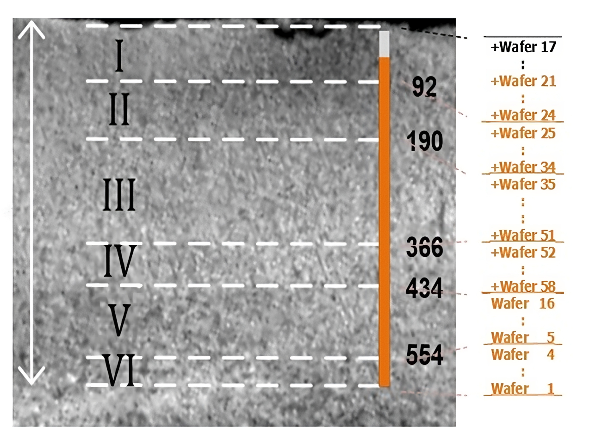
Figure 5: The relative positions of the wafer layers selected from the MEC dataset.

D.2 Metrics

Variation of Information (VOI) is an information-theoretic measure that assesses the distance between two clusterings in terms of their average conditional entropy. Given the predicted segmentation $S_{pred}$ and the ground-truth segmentation $S_{gt}$, VOI is defined as:

$$VOI(S_{pred},S_{gt})=H(S_{pred}|S_{gt})+H(S_{gt}|S_{pred}),$$ (39)

where $H(\cdot|\cdot)$ denotes the conditional entropy. It can be calculated by:

$$H(S_{pred}|S_{gt})=-\sum_{i=1}^{|S_{gt}|}\sum_{j=1}^{|S_{pred}|}\frac{|S_{gt}^{i}\cap S_{pred}^{j}|}{N}\log\frac{|S_{gt}^{i}\cap S_{pred}^{j}|}{|S_{gt}^{i}|},$$ (40)

where $S_{gt}^{i}$ and $S_{pred}^{j}$ represent the $i$-th and $j$-th segments in the ground-truth and predicted segmentation, respectively, and $N$ is the total number of voxels. VOI ranges from 0 to $\infty$, with a lower value indicating better segmentation performance.

Adjusted Rand Index (ARAND) is a variant of the Rand Index arganda2015crowdsourcing that corrects for chance when comparing two clusterings. It is defined as:

$$ARAND(S_{pred},S_{gt})=\frac{\sum_{ij}\binom{n_{ij}}{2}-[\sum_{i}\binom{a_{i}}{2}\sum_{j}\binom{b_{j}}{2}]/\binom{N}{2}}{[\sum_{i}\binom{a_{i}}{2}+\sum_{j}\binom{b_{j}}{2}]/2-[\sum_{i}\binom{a_{i}}{2}\sum_{j}\binom{b_{j}}{2}]/\binom{N}{2}},$$ (41)

where $n_{ij}$ is the number of voxels that are in segment $i$ of $S_{pred}$ and segment $j$ of $S_{gt}$, $a_{i}=\sum_{j}n_{ij}$ is the number of voxels in segment $i$ of $S_{pred}$, $b_{j}=\sum_{i}n_{ij}$ is the number of voxels in segment $j$ of $S_{gt}$, and $N=\sum_{ij}n_{ij}$ is the total number of voxels. ARAND ranges from 0 to 1, with a lower value indicating better segmentation performance.

Appendix E Discussion

E.1 Limitations

Despite TokenUnify’s significant performance advantages in long-sequence autoregressive tasks, this may be attributed to the specific characteristics of 3D image sequences. Its effectiveness on natural images has yet to be validated in downstream tasks. Additionally, due to the unique nature of the neuron data, we have only demonstrated performance on segmentation tasks in the main text. Future work will extend the evaluation to a broader set of downstream tasks, such as classification, detection, and other standard vision tasks.

E.2 Preliminary Exploration of TokenUnify on Natural Images

We are currently pretraining TokenUnify on natural images using the LAION-5B dataset schuhmann2022laion . Specifically, each image is divided into non-overlapping patches of size 16x16. We conducted 800 epochs of pretraining with TokenUnify. As the downstream classification tasks are still in progress, we present only the initial visual results here.

Specifically, we pretrained using both the Autoregress approach and the TokenUnify approach. For evaluation, given the first k patches of an image, we predicted the (k+1)th patch and then concatenated all the predicted patches. We used the PSNR metric to compare the reconstructed image with the original image, assessing the representational capability of each method. We selected the high-resolution Kodak kodak1993suite dataset as our test set. Our experimental results are shown in Fig. 6. The PSNR values for the reconstruction of 24 images are detailed in Table 4. TokenUnify outperformed the Autoregress approach in terms of visual metrics, indicating that TokenUnify likely extracted better visual representations during the pretraining stage.

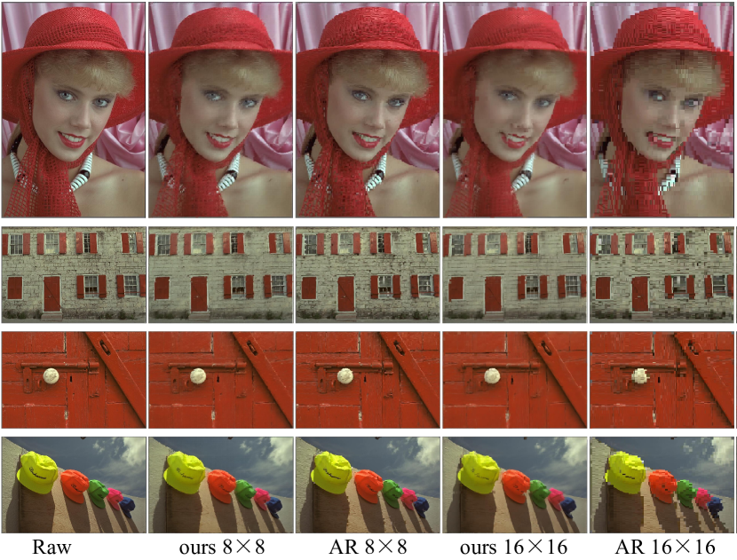
Figure 6: Shows the reconstruction result of selected Kodak dataset, images are divided into different sizes of patches. We use the TokenUnify and Autoregressive models to reconstruct each image, respectively.

Table 4: Presents the PSNR results of reconstructing 24 images from the Kodak dataset using TokenUnify and Autoregress. The experiments were conducted with patch sizes of 16x16 and 8x8.

Kodak Name	16$\times$16 Autoregress	16$\times$16 TokenUnify	8$\times$8 Autoregress	8$\times$8 TokenUnify
1.png	19.249	21.549 (+2.300)	21.247	21.990 (+0.743)
2.png	24.662	27.321 (+2.659)	27.269	27.799 (+0.530)
3.png	22.665	27.113 (+4.448)	26.851	28.110 (+1.259)
4.png	22.353	26.152 (+3.799)	25.466	26.713 (+1.247)
5.png	15.353	18.859 (+3.506)	18.437	19.847 (+1.410)
6.png	20.139	22.376 (+2.237)	21.661	23.064 (+1.403)
7.png	19.990	23.170 (+3.180)	23.334	24.479 (+1.145)
8.png	15.146	18.169 (+3.023)	17.829	18.770 (+0.941)
9.png	22.080	24.918 (+2.838)	24.959	25.957 (+0.998)
10.png	22.239	25.213 (+2.974)	25.042	25.936 (+0.894)
11.png	20.289	22.536 (+2.247)	22.638	23.723 (+1.085)
12.png	21.854	25.929 (+4.075)	25.806	27.005 (+1.199)
13.png	15.946	18.494 (+2.548)	17.657	18.969 (+1.312)
14.png	18.107	21.227 (+3.120)	20.696	22.195 (+1.499)
15.png	20.750	24.659 (+3.909)	25.321	26.111 (+0.790)
16.png	23.216	25.887 (+2.671)	25.334	26.694 (+1.360)
17.png	20.672	24.346 (+3.674)	24.220	25.614 (+1.394)
18.png	19.959	22.017 (+2.058)	21.249	22.336 (+1.087)
19.png	22.394	25.062 (+2.668)	24.094	25.384 (+1.290)
20.png	21.478	24.723 (+3.245)	24.124	25.346 (+1.222)
21.png	17.503	20.149 (+2.646)	19.567	20.366 (+0.799)
22.png	19.947	23.003 (+3.056)	22.365	23.545 (+1.180)
23.png	17.807	20.315 (+2.508)	19.781	20.959 (+1.178)
24.png	22.111	24.780 (+2.669)	24.313	25.472 (+1.159)

Appendix F Mehtod Details

F.1 Summary of the TokenUnify Algorithm

TokenUnify is a novel pre-training method for scalable autoregressive visual modeling. It integrates random token prediction, next-token prediction, and next-all token prediction to mitigate cumulative errors in visual autoregression while maintaining favorable scaling laws. The algorithm leverages the Mamba network architecture to reduce computational complexity from quadratic to linear for long-sequence modeling.

1

Input : Unlabeled image data $X=\{X^{(1)},\dots,X^{(T)}\}$

Input : Model parameters $\theta_{1}$

Output : Pre-trained model $f_{\theta_{1}}(\cdot)$

2

3for $t\leftarrow 1$ to $T$ do

4        Partition $X^{(t)}$ into patches $\{x_{1},\dots,x_{K}\}$

5        Tokenize patches: $\{x_{1},\dots,x_{K}\}\rightarrow\text{tokens}$

6        Compute loss functions:

7        Random token prediction: $\mathcal{L}_{\text{random}}=-\sum_{i\in M}\log p(x_{i}\mid x_{\bar{M}})$

8        Next token prediction: $\mathcal{L}_{\text{next}}=-\sum_{i=1}^{K}\log p(x_{i}\mid x_{<i})$

9        Next-all token prediction: $\mathcal{L}_{\text{next-all}}=-\sum_{i=1}^{K}\sum_{j=i}^{K}\log p(x_{j}\mid x_{<i})$

10        Update $\theta_{1}$ to minimize $\mathcal{L}_{\text{random}}$, $\mathcal{L}_{\text{next}}$, $\mathcal{L}_{\text{next-all}}$

11

return $f_{\theta_{1}}(\cdot)$

Algorithm 1 TokenUnify Pre-training

Pre-training is conducted on a large-scale, ultra-high-resolution electron microscopy (EM) image dataset, providing spatially correlated long sequences. TokenUnify demonstrates significant improvements in segmentation performance on downstream EM neuron segmentation tasks compared to existing methods. Our pre-training and fine-tuning algorithms are summarized in Algorithm 1 and Algorithm 2, respectively.

1

Input : Labeled data $\mathcal{D}_{l}=\{(x_{i}^{l},y_{i})\}_{i=1}^{|\mathcal{D}_{l}|}$

Input : Pre-trained model $f_{\theta_{1}}(\cdot)$

Input : Segmentation model $g_{\theta_{2}}(\cdot)$

Output : Fine-tuned segmentation model $g_{\theta_{2}}(\cdot)$

2

3Initialize $\theta_{2}$ with $\theta_{1}$

4 for $i\leftarrow 1$ to $|\mathcal{D}_{l}|$ do

5        $\hat{y}_{i}=g_{\theta_{2}}(f_{\theta_{1}}(x_{i}^{l}))$

6        $\mathcal{L}_{\text{seg}}=\frac{1}{|\mathcal{D}_{l}|}\sum_{i=1}^{|\mathcal{D}_{l}|}|\hat{y}_{i}-y_{i}|^{2}$

7        Update $\theta_{2}$ to minimize $\mathcal{L}_{\text{seg}}$

8

return $g_{\theta_{2}}(\cdot)$

Algorithm 2 TokenUnify Fine-tuning

The TokenUnify pre-training algorithm captures both local and global dependencies in image data through mixed token prediction tasks. The Mamba network architecture ensures efficient modeling of long sequences. During fine-tuning, the pre-trained model adapts to downstream segmentation tasks using labeled data, achieving state-of-the-art performance on EM neuron segmentation benchmarks.

F.2 Perceiver Resampler

The workflow of the Perceiver Resampler alayrac2022flamingo ; chen2024automated ; chen2023quantifying can be summarized in the following steps: 1. Combine the output of the Vision Encoder (e.g., features from images) with learned time position encodings. 2. Flatten the combined features into a one-dimensional sequence. 3. Flatten the combined features into a one-dimensional sequence. 4. Process the flattened features using Transformer layers that incorporate attention mechanisms, which interact with learned latent query vectors. Output a fixed number of visual tokens equal to the number of latent queries.

1

Input : $\mathbf{x}_{f}$ - The [T, S, d] visual features (T=time, S=space)

Input : $\mathbf{t}$ - The [T, 1, d] time position embeddings

Input : $\mathbf{x}$ - R learned latents of shape [R, d]

Input : num_layers - Number of layers

Output : $\mathbf{x}$ - Updated learned latents

2

3Add time position embeddings and flatten:

4 $\mathbf{x}_{f}\leftarrow\mathbf{x}_{f}+\mathbf{t}$

5 $\mathbf{x}_{f}\leftarrow\text{flatten}(\mathbf{x}_{f})$

6     // $[T,S,d]\rightarrow[T\times S,d]$

7Apply the Perceiver Resampler layers:

8 for $i\leftarrow 1$ to num_layers do

9        $\mathbf{x}\leftarrow\mathbf{x}+\text{attention}_{i}(q=\mathbf{x},kv=\text{concat}([\mathbf{x}_{f},\mathbf{x}]))$

10        $\mathbf{x}\leftarrow\mathbf{x}+\text{ffw}_{i}(\mathbf{x})$

11

return $\mathbf{x}$

Algorithm 3 Perceiver Resampler Pseudocode

The input visual features, denoted as $\mathbf{x}_{f}$, have a shape of $[T,S,d]$, where $T$ represents the time dimension, $S$ the spatial dimension, and $d$ the feature dimension. The time position embeddings, represented by $\mathbf{t}$, are of shape $[T,1,d]$ and are added to the visual features to incorporate temporal information.

The learned latents, denoted as $\mathbf{x}$, have a shape of $[R,d]$, where $R$ is the number of latents and $d$ is the feature dimension. The parameter num_layers specifies the number of layers in the Perceiver Resampler model.

The operation flatten reshapes the input tensor from $[T,S,d]$ to $[T\times S,d]$. The function attention_i represents the attention mechanism applied in the $i$-th layer, which takes a query $q$ and key-value pairs $kv$. The function concat concatenates the input tensors along the specified dimension. Finally, ffw_i refers to the feedforward network applied in the $i$-th layer.

F.3 Segmentation Method

The EMmamba network is structured into three principal components: 3D feature encoder, convolution-based decoder for segmentation prediction, and skip connections to integrate local multi-scale features into the decoder for feature fusion. liu2023deep ; liu2023toothsegnet ; sun2024eagle

To achieve effective feature encoding, we designed anisotropic downsampling layers and adopted the TSMamba block from the Segmamba xing2024segmamba . Specifically, in Stage 1, the downsampling layer uses a convolutional kernel size of (1, 7, 7). For the subsequent three layers, the downsampling layers have a convolutional kernel size of (1, 2, 2). The decoder section employs a convolutional kernel size of (1, 5, 5). This anisotropic design is particularly advantageous for processing EM images, which exhibit inherent anisotropy.

Table 5: Shows the differ in architecture when adding the parameters of the segmentation backbone.

	EMmamba-tiny	EMmamba-small	EMmamba-middle	EMmamba-large	EMmamba-huge
Mamba layer	[2,2,2,2]	[2,2,2,2]	[2,2,2,2]	[2,2,2,2]	[2,2,2,2]
Feature size	[32,64,128,256]	[64,128,256,512]	[96,192,384,768]	[144,288,576,1104]	[192,384,768,1536]
Hidden size	512	1024	1024	2048	3072
Kernel size	[1,5,5]	[1,5,5]	[1,5,5]	[1,5,5]	[1,5,5]
Batch size	40	22	12	8	4
Param. (M)	28.30	112.5	206.6	506.6	1008

Appendix G Numerical Results

G.1 Statistical Test

In this section, we present the results of our error bar experiments, as detailed in Table 8. These experiments were conducted to assess the variability and reliability of the model’s prediction under different conditions.

Table 6: Ablation study for different pertaining strategy on wafer4 dataset.

Model	Pretraining Strategy			$VOI\downarrow$	$ARAND\downarrow$
	Random token	Next token	Next-all token
M1	✓			1.2680	0.0862
M2	✓	✓		1.1300	0.0692
M3	✓		✓	1.1907	0.1203
Ours	✓	✓	✓	0.9951	0.0509

Table 7: Ablation study for the fine-tuning schemes on wafer4 dataset.

Model	Module			$VOI\downarrow$	$ARAND\downarrow$
	Mamba	Encoder	Decoder
M1	✓			1.1362	0.0782
M2		✓		1.5556	0.1370
M3			✓	1.5295	0.1212
M4	✓	✓		1.1065	0.0629
Ours	✓	✓	✓	0.9951	0.0509

Table 8: Quantitative comparison of segmentation results on Wafer4 dataset with error bar. ‘Post.’ represents the post-processing algorithms. * denotes the MAE pretraining strategy he2022masked . † indicates our TokenUnify pretraining strategy. The best results are in bold and the second best results are in underlined.

Post.	Method	Wafer4				Param.
Waterz funke2018large		$VOI_{M}\downarrow$	$VOI_{S}\downarrow$	$VOI\downarrow$	$ARAND\downarrow$	(M)
	Superhuman lee2017superhuman	0.3392$\pm$0.0167	1.2247$\pm$0.0857	1.5639$\pm$0.0921	0.2050$\pm$0.0284	1.478
	MALA funke2018large	0.6217$\pm$0.1266	1.5314$\pm$0.1123	2.1531$\pm$0.1004	0.1490$\pm$0.0476	84.02
	PEA huang2022learning	0.3943$\pm$0.0655	1.0036$\pm$0.1435	2.1531$\pm$0.1004	0.1490$\pm$0.0476	1.480
	UNETR hatamizadeh2022unetr	0.4454$\pm$0.0155	1.7979$\pm$0.1548	2.2433$\pm$0.1424	0.3244$\pm$0.0701	129.1
	EMmamba	0.4353$\pm$0.052	1.3018$\pm$0.0086	1.7371$\pm$0.0432	0.1872$\pm$0.0156	28.30
	Superhuman*	0.2907$\pm$0.0063	0.9437$\pm$0.0451	1.2344$\pm$0.0388	0.1202$\pm$0.0121	1.478
	MALA*	0.7732$\pm$0.1432	1.2063$\pm$0.0458	1.9768$\pm$0.1232	0.2663$\pm$0.0549	84.02
	PEA*	0.2712$\pm$0.0185	0.9715$\pm$0.1841	1.2427$\pm$0.1963	0.0805$\pm$0.0386	1.480
	UNETR*	0.3554$\pm$0.0411	0.8579$\pm$0.0229	1.2133$\pm$0.0574	0.1150$\pm$0.0209	129.1
	EMmamba*	0.2363$\pm$0.0212	1.0782$\pm$0.0251	1.3144$\pm$0.0444	0.0967$\pm$0.0097	28.30
	EMmamba†	0.2124$\pm$0.0172	0.8047$\pm$0.0057	1.0024$\pm$0.0463	0.0551$\pm$0.0040	28.30
LMC beier2017multicut	Superhuman lee2017superhuman	0.2006$\pm$0.0054	2.1283$\pm$0.1378	2.3289$\pm$0.1427	0.2924$\pm$0.0408	1.478
	MALA funke2018large	0.3094$\pm$0.0478	2.3802$\pm$0.1863	2.6869$\pm$0.1558	0.2303$\pm$0.0314	84.02
	PEA huang2022learning	0.2303$\pm$0.0870	1.6373$\pm$0.1289	1.8343$\pm$0.0732	0.1611$\pm$0.0152	1.480
	UNETR hatamizadeh2022unetr	0.1625$\pm$0.0144	3.3146$\pm$0.1391	3.4772$\pm$0.1272	0.6600$\pm$0.0304	129.1
	EMmamba	0.1594$\pm$0.0005	2.0921$\pm$0.0300	2.2515$\pm$0.0298	0.2104$\pm$0.0113	28.30
	Superhuman*	0.2363$\pm$0.0222	1.8475$\pm$0.0781	2.0838$\pm$0.0782	0.1946$\pm$0.0171	1.478
	MALA*	0.2022$\pm$0.0089	2.5760$\pm$0.0457	2.8117$\pm$0.0346	0.5695$\pm$0.0183	84.02
	PEA*	0.2736$\pm$0.1603	1.5868$\pm$0.0900	1.8604$\pm$0.0815	0.1386$\pm$0.0134	1.480
	UNETR*	0.1829$\pm$0.0495	1.7723$\pm$0.0324	1.9552$\pm$0.0816	0.1372$\pm$0.0316	129.1
	EMmamba*	0.1342$\pm$0.0020	1.9014$\pm$0.0286	2.0356$\pm$0.0301	0.1420$\pm$0.0023	28.30
	EMmamba†	0.1417$\pm$0.0022	1.5186$\pm$0.0076	1.6604$\pm$0.0086	0.0592$\pm$0.0002	28.30

G.2 Abalation Study Results

In this section, we present the numerical results of the ablation study discussed in Section 5.

References

- [1] Josh Achiam, Steven Adler, Sandhini Agarwal, Lama Ahmad, Ilge Akkaya, Florencia Leoni Aleman, Diogo Almeida, Janko Altenschmidt, Sam Altman, Shyamal Anadkat, et al. Gpt-4 technical report. arXiv preprint arXiv:2303.08774, 2023.
- [2] Jean-Baptiste Alayrac, Jeff Donahue, Pauline Luc, Antoine Miech, Iain Barr, Yana Hasson, Karel Lenc, Arthur Mensch, Katherine Millican, Malcolm Reynolds, et al. Flamingo: a visual language model for few-shot learning. In NeurIPS, volume 35, pages 23716--23736, 2022.
- [3] Ignacio Arganda-Carreras, Srinivas C Turaga, Daniel R Berger, Dan Cireşan, Alessandro Giusti, Luca M Gambardella, Jürgen Schmidhuber, Dmitry Laptev, Sarvesh Dwivedi, Joachim M Buhmann, et al. Crowdsourcing the creation of image segmentation algorithms for connectomics. Frontiers in neuroanatomy, 9:152591, 2015.
- [4] Gregor Bachmann and Vaishnavh Nagarajan. The pitfalls of next-token prediction. arXiv preprint arXiv:2403.06963, 2024.
- [5] Jinze Bai, Shuai Bai, Yunfei Chu, Zeyu Cui, Kai Dang, Xiaodong Deng, Yang Fan, Wenbin Ge, Yu Han, Fei Huang, et al. Qwen technical report. arXiv preprint arXiv:2309.16609, 2023.
- [6] Jinze Bai, Shuai Bai, Shusheng Yang, Shijie Wang, Sinan Tan, Peng Wang, Junyang Lin, Chang Zhou, and Jingren Zhou. Qwen-vl: A versatile vision-language model for understanding, localization, text reading, and beyond. arXiv preprint arXiv:2308.12966, 2023.
- [7] Yutong Bai, Xinyang Geng, Karttikeya Mangalam, Amir Bar, Alan Yuille, Trevor Darrell, Jitendra Malik, and Alexei A Efros. Sequential modeling enables scalable learning for large vision models. arXiv preprint arXiv:2312.00785, 2023.
- [8] Thorsten Beier, Constantin Pape, Nasim Rahaman, Timo Prange, Stuart Berg, Davi D Bock, Albert Cardona, Graham W Knott, Stephen M Plaza, Louis K Scheffer, et al. Multicut brings automated neurite segmentation closer to human performance. Nature methods, 14(2):101--102, 2017.
- [9] Samy Bengio, Oriol Vinyals, Navdeep Jaitly, and Noam Shazeer. Scheduled sampling for sequence prediction with recurrent neural networks. In NeurIPS, volume 28, 2015.
- [10] Tom Brown, Benjamin Mann, Nick Ryder, Melanie Subbiah, Jared D Kaplan, Prafulla Dhariwal, Arvind Neelakantan, Pranav Shyam, Girish Sastry, Amanda Askell, et al. Language models are few-shot learners. In NeurIPS, volume 33, pages 1877--1901, 2020.
- [11] Jiuhai Chen and Jonas Mueller. Quantifying uncertainty in answers from any language model via intrinsic and extrinsic confidence assessment. arXiv preprint arXiv:2308.16175, 2023.
- [12] Jiuhai Chen and Jonas Mueller. Automated data curation for robust language model fine-tuning. arXiv preprint arXiv:2403.12776, 2024.
- [13] Junbo Chen, Xupeng Chen, Ran Wang, Chenqian Le, Amirhossein Khalilian-Gourtani, Erika Jensen, Patricia Dugan, Werner Doyle, Orrin Devinsky, Daniel Friedman, et al. Subject-agnostic transformer-based neural speech decoding from surface and depth electrode signals. bioRxiv, pages 2024--03, 2024.
- [14] Mark Chen, Alec Radford, Rewon Child, Jeffrey Wu, Heewoo Jun, David Luan, and Ilya Sutskever. Generative pretraining from pixels. In ICML, pages 1691--1703. PMLR, 2020.
- [15] Yinda Chen, Wei Huang, Xiaoyu Liu, Shiyu Deng, Qi Chen, and Zhiwei Xiong. Learning multiscale consistency for self-supervised electron microscopy instance segmentation. In ICASSP, pages 1566--1570. IEEE, 2024.
- [16] Yinda Chen, Wei Huang, Shenglong Zhou, Qi Chen, and Zhiwei Xiong. Self-supervised neuron segmentation with multi-agent reinforcement learning. In IJCAI, pages 609--617, 2023.
- [17] Yinda Chen, Che Liu, Wei Huang, Sibo Cheng, Rossella Arcucci, and Zhiwei Xiong. Generative text-guided 3d vision-language pretraining for unified medical image segmentation. arXiv preprint arXiv:2306.04811, 2023.
- [18] Yinda Chen, Che Liu, Xiaoyu Liu, Rossella Arcucci, and Zhiwei Xiong. Bimcv-r: A landmark dataset for 3d ct text-image retrieval. arXiv preprint arXiv:2403.15992, 2024.
- [19] Z Chen and L Jing. Multimodal semi-supervised learning for 3d objects. In The British Machine Vision Conference (BMVC), 2021.
- [20] Zhimin Chen, Longlong Jing, Yingwei Li, and Bing Li. Bridging the domain gap: Self-supervised 3d scene understanding with foundation models. Advances in Neural Information Processing Systems, 36, 2024.
- [21] Zhimin Chen, Longlong Jing, Liang Yang, Yingwei Li, and Bing Li. Class-level confidence based 3d semi-supervised learning. In Proceedings of the IEEE/CVF Winter Conference on Applications of Computer Vision, pages 633--642, 2023.
- [22] Zhimin Chen, Yingwei Li, Longlong Jing, Liang Yang, and Bing Li. Point cloud self-supervised learning via 3d to multi-view masked autoencoder. arXiv preprint arXiv:2311.10887, 2023.
- [23] Wenliang Dai, Junnan Li, Dongxu Li, Anthony Meng Huat Tiong, Junqi Zhao, Weisheng Wang, Boyang Li, Pascale N Fung, and Steven Hoi. Instructblip: Towards general-purpose vision-language models with instruction tuning. In NeurIPS, volume 36, 2024.
- [24] Bo Dang, Wenchao Zhao, Yufeng Li, Danqing Ma, Qixuan Yu, and Elly Yijun Zhu. Real-time pill identification for the visually impaired using deep learning. arXiv preprint arXiv:2405.05983, 2024.
- [25] Jacob Devlin, Ming-Wei Chang, Kenton Lee, and Kristina Toutanova. Bert: Pre-training of deep bidirectional transformers for language understanding. arXiv preprint arXiv:1810.04805, 2018.
- [26] Zhiyuan Ding, Qi Dong, Haote Xu, Chenxin Li, Xinghao Ding, and Yue Huang. Unsupervised anomaly segmentation for brain lesions using dual semantic-manifold reconstruction. In ICONIP, 2022.
- [27] Alaaeldin El-Nouby, Michal Klein, Shuangfei Zhai, Miguel Angel Bautista, Alexander Toshev, Vaishaal Shankar, Joshua M Susskind, and Armand Joulin. Scalable pre-training of large autoregressive image models. arXiv preprint arXiv:2401.08541, 2024.
- [28] J Funke, S Saalfeld, DD Bock, SC Turaga, and E Perlman. Miccai challenge on circuit reconstruction from electron microscopy images. In MICCAI, 2016.
- [29] Jan Funke, Fabian Tschopp, William Grisaitis, Arlo Sheridan, Chandan Singh, Stephan Saalfeld, and Srinivas C Turaga. Large scale image segmentation with structured loss based deep learning for connectome reconstruction. IEEE transactions on pattern analysis and machine intelligence, 41(7):1669--1680, 2018.
- [30] Albert Gu and Tri Dao. Mamba: Linear-time sequence modeling with selective state spaces. arXiv preprint arXiv:2312.00752, 2023.
- [31] Ali Hatamizadeh, Yucheng Tang, Vishwesh Nath, Dong Yang, Andriy Myronenko, Bennett Landman, Holger R Roth, and Daguang Xu. Unetr: Transformers for 3d medical image segmentation. In WACV, pages 574--584, 2022.
- [32] Kaiming He, Xinlei Chen, Saining Xie, Yanghao Li, Piotr Dollár, and Ross Girshick. Masked autoencoders are scalable vision learners. In CVPR, pages 16000--16009, 2022.
- [33] Kaiming He, Haoqi Fan, Yuxin Wu, Saining Xie, and Ross Girshick. Momentum contrast for unsupervised visual representation learning. In CVPR, pages 9729--9738, 2020.
- [34] Edward J Hu, Yelong Shen, Phillip Wallis, Zeyuan Allen-Zhu, Yuanzhi Li, Shean Wang, Lu Wang, and Weizhu Chen. LoRA: Low-rank adaptation of large language models. In ICLR, 2022.
- [35] Wei Huang, Shiyu Deng, Chang Chen, Xueyang Fu, and Zhiwei Xiong. Learning to model pixel-embedded affinity for homogeneous instance segmentation. In AAAI, volume 36, pages 1007--1015, 2022.
- [36] Narayanan Kasthuri, Kenneth Jeffrey Hayworth, Daniel Raimund Berger, Richard Lee Schalek, José Angel Conchello, Seymour Knowles-Barley, Dongil Lee, Amelio Vázquez-Reina, Verena Kaynig, Thouis Raymond Jones, et al. Saturated reconstruction of a volume of neocortex. Cell, 162(3):648--661, 2015.
- [37] Brian W Kernighan and Shen Lin. An efficient heuristic procedure for partitioning graphs. The Bell system technical journal, 49(2):291--307, 1970.
- [38] E. Kodak. Kodak lossless true color image suite (photocd pcd0992), 1993. Version 5.
- [39] Jinhyuk Lee, Wonjin Yoon, Sungdong Kim, Donghyeon Kim, Sunkyu Kim, Chan Ho So, and Jaewoo Kang. Biobert: a pre-trained biomedical language representation model for biomedical text mining. Bioinformatics, 36(4):1234--1240, 2020.
- [40] Kisuk Lee, Jonathan Zung, Peter Li, Viren Jain, and H Sebastian Seung. Superhuman accuracy on the snemi3d connectomics challenge. arXiv preprint arXiv:1706.00120, 2017.
- [41] Chenxin Li, Yunlong Zhang, Zhehan Liang, Wenao Ma, Yue Huang, and Xinghao Ding. Consistent posterior distributions under vessel-mixing: a regularization for cross-domain retinal artery/vein classification. In 2021 IEEE International Conference on Image Processing (ICIP), pages 61--65. IEEE, 2021.
- [42] Junnan Li, Dongxu Li, Silvio Savarese, and Steven Hoi. Blip-2: Bootstrapping language-image pre-training with frozen image encoders and large language models. In ICML, pages 19730--19742. PMLR, 2023.
- [43] Junnan Li, Dongxu Li, Caiming Xiong, and Steven Hoi. Blip: Bootstrapping language-image pre-training for unified vision-language understanding and generation. In ICML, pages 12888--12900. PMLR, 2022.
- [44] Panfeng Li, Mohamed Abouelenien, and Rada Mihalcea. Deception detection from linguistic and physiological data streams using bimodal convolutional neural networks. arXiv preprint arXiv:2311.10944, 2023.
- [45] Panfeng Li, Youzuo Lin, and Emily Schultz-Fellenz. Contextual hourglass network for semantic segmentation of high resolution aerial imagery. arXiv preprint arXiv:1810.12813, 2018.
- [46] Panfeng Li, Qikai Yang, Xieming Geng, Wenjing Zhou, Zhicheng Ding, and Yi Nian. Exploring diverse methods in visual question answering. arXiv preprint arXiv:2404.13565, 2024.
- [47] Tianhong Li, Huiwen Chang, Shlok Mishra, Han Zhang, Dina Katabi, and Dilip Krishnan. Mage: Masked generative encoder to unify representation learning and image synthesis. In CVPR, pages 2142--2152, 2023.
- [48] Yufeng Li, Weimin Wang, Xu Yan, Min Gao, and MingXuan Xiao. Research on the application of semantic network in disease diagnosis prompts based on medical corpus. International Journal of Innovative Research in Computer Science & Technology, 12(2):1--9, 2024.
- [49] Che Liu, Cheng Ouyang, Yinda Chen, Cesar César Quilodrán-Casas, Lei Ma, Jie Fu, Yike Guo, Anand Shah, Wenjia Bai, and Rossella Arcucci. T3d: Towards 3d medical image understanding through vision-language pre-training. arXiv preprint arXiv:2312.01529, 2023.
- [50] Jiaxiang Liu, Jin Hao, Hangzheng Lin, Wei Pan, Jianfei Yang, Yang Feng, Gaoang Wang, Jin Li, Zuolin Jin, Zhihe Zhao, et al. Deep learning-enabled 3d multimodal fusion of cone-beam ct and intraoral mesh scans for clinically applicable tooth-bone reconstruction. Patterns, 4(9), 2023.
- [51] Jiaxiang Liu, Tianxiang Hu, Yang Feng, Wanghui Ding, and Zuozhu Liu. Toothsegnet: image degradation meets tooth segmentation in cbct images. In 2023 IEEE 20th International Symposium on Biomedical Imaging (ISBI), pages 1--5. IEEE, 2023.
- [52] Jiaxiang Liu, Tianxiang Hu, Yan Zhang, Yang Feng, Jin Hao, Junhui Lv, and Zuozhu Liu. Parameter-efficient transfer learning for medical visual question answering. IEEE Transactions on Emerging Topics in Computational Intelligence, 2023.
- [53] Ilya Loshchilov and Frank Hutter. Decoupled weight decay regularization. In ICLR, 2018.
- [54] Jiasen Lu, Christopher Clark, Sangho Lee, Zichen Zhang, Savya Khosla, Ryan Marten, Derek Hoiem, and Aniruddha Kembhavi. Unified-io 2: Scaling autoregressive multimodal models with vision, language, audio, and action. arXiv preprint arXiv:2312.17172, 2023.
- [55] Juan Nunez-Iglesias, Ryan Kennedy, Toufiq Parag, Jianbo Shi, and Dmitri B Chklovskii. Machine learning of hierarchical clustering to segment 2d and 3d images. PloS one, 8(8):e71715, 2013.
- [56] Maxime Oquab, Timothée Darcet, Théo Moutakanni, Huy V Vo, Marc Szafraniec, Vasil Khalidov, Pierre Fernandez, Daniel HAZIZA, Francisco Massa, Alaaeldin El-Nouby, et al. Dinov2: Learning robust visual features without supervision. Transactions on Machine Learning Research, 2023.
- [57] Alec Radford, Jong Wook Kim, Chris Hallacy, Aditya Ramesh, Gabriel Goh, Sandhini Agarwal, Girish Sastry, Amanda Askell, Pamela Mishkin, Jack Clark, et al. Learning transferable visual models from natural language supervision. In ICML, pages 8748--8763. PMLR, 2021.
- [58] Alec Radford, Jeffrey Wu, Rewon Child, David Luan, Dario Amodei, Ilya Sutskever, et al. Language models are unsupervised multitask learners. OpenAI blog, 1(8):9, 2019.
- [59] Philipp Schlegel, Alexander S Bates, Tejal Parag, Gregory SXE Jefferis, and Davi D Bock. Automatic detection of synaptic partners in a whole-brain drosophila em dataset. Nature Methods, 18(8):877–884, 2021.
- [60] Christoph Schuhmann, Romain Beaumont, Richard Vencu, Cade Gordon, Ross Wightman, Mehdi Cherti, Theo Coombes, Aarush Katta, Clayton Mullis, Mitchell Wortsman, et al. Laion-5b: An open large-scale dataset for training next generation image-text models. In NeurIPS, volume 35, pages 25278--25294, 2022.
- [61] Mannat Singh, Quentin Duval, Kalyan Vasudev Alwala, Haoqi Fan, Vaibhav Aggarwal, Aaron Adcock, Armand Joulin, Piotr Dollár, Christoph Feichtenhofer, Ross Girshick, et al. The effectiveness of mae pre-pretraining for billion-scale pretraining. In ICCV, pages 5484--5494, 2023.
- [62] Xingchen Song, Di Wu, Binbin Zhang, Zhendong Peng, Bo Dang, Fuping Pan, and Zhiyong Wu. ZeroPrompt: Streaming Acoustic Encoders are Zero-Shot Masked LMs. In INTERSPEECH, pages 1648--1652, 2023.
- [63] Yipeng Sun, Yixing Huang, Linda-Sophie Schneider, Mareike Thies, Mingxuan Gu, Siyuan Mei, Siming Bayer, and Andreas Maier. Eagle: An edge-aware gradient localization enhanced loss for ct image reconstruction. arXiv preprint arXiv:2403.10695, 2024.
- [64] Shin-ya Takemura, Yoshinori Aso, Toshihide Hige, Allan Wong, Zhiyuan Lu, C Shan Xu, Patricia K Rivlin, Harald Hess, Ting Zhao, Toufiq Parag, et al. A connectome of a learning and memory center in the adult drosophila brain. Elife, 6:e26975, 2017.
- [65] Hugo Touvron, Thibaut Lavril, Gautier Izacard, Xavier Martinet, Marie-Anne Lachaux, Timothée Lacroix, Baptiste Rozière, Naman Goyal, Eric Hambro, Faisal Azhar, et al. Llama: Open and efficient foundation language models. arXiv preprint arXiv:2302.13971, 2023.
- [66] Hugo Touvron, Louis Martin, Kevin Stone, Peter Albert, Amjad Almahairi, Yasmine Babaei, Nikolay Bashlykov, Soumya Batra, Prajjwal Bhargava, Shruti Bhosale, et al. Llama 2: Open foundation and fine-tuned chat models. arXiv preprint arXiv:2307.09288, 2023.
- [67] Ran Wang, Xupeng Chen, Amirhossein Khalilian-Gourtani, Leyao Yu, Patricia Dugan, Daniel Friedman, Werner Doyle, Orrin Devinsky, Yao Wang, and Adeen Flinker. Distributed feedforward and feedback cortical processing supports human speech production. Proceedings of the National Academy of Sciences, 120(42):e2300255120, 2023.
- [68] Zifeng Wang, Zhenbang Wu, Dinesh Agarwal, and Jimeng Sun. Medclip: Contrastive learning from unpaired medical images and text. In EMNLP, pages 3876--3887, 2022.
- [69] Donglai Wei, Zudi Lin, Daniel Franco-Barranco, Nils Wendt, Xingyu Liu, Wenjie Yin, Xin Huang, Aarush Gupta, Won-Dong Jang, Xueying Wang, et al. Mitoem dataset: Large-scale 3d mitochondria instance segmentation from em images. In Miccai, pages 66--76. Springer, 2020.
- [70] Patrick Xia, Shijie Wu, and Benjamin Van Durme. Which* bert? a survey organizing contextualized encoders. In EMNLP, pages 7516--7533, 2020.
- [71] Ao Xiang, Jingyu Zhang, Qin Yang, Liyang Wang, and Yu Cheng. Research on splicing image detection algorithms based on natural image statistical characteristics. arXiv preprint arXiv:2404.16296, 2024.
- [72] Zhaohu Xing, Tian Ye, Yijun Yang, Guang Liu, and Lei Zhu. Segmamba: Long-range sequential modeling mamba for 3d medical image segmentation. arXiv preprint arXiv:2401.13560, 2024.
- [73] Jure Zbontar, Li Jing, Ishan Misra, Yann LeCun, and Stéphane Deny. Barlow twins: Self-supervised learning via redundancy reduction. In ICML, pages 12310--12320. PMLR, 2021.
- [74] Biao Zhang and Rico Sennrich. Root mean square layer normalization. In NeurIPS, volume 32, 2019.
- [75] Jingyu Zhang, Ao Xiang, Yu Cheng, Qin Yang, and Liyang Wang. Research on detection of floating objects in river and lake based on ai intelligent image recognition. arXiv preprint arXiv:2404.06883, 2024.
- [76] Sheng Zhang, Yanbo Xu, Naoto Usuyama, Jaspreet Bagga, Robert Tinn, Sam Preston, Rajesh Rao, Mu Wei, Naveen Valluri, Cliff Wong, et al. Large-scale domain-specific pretraining for biomedical vision-language processing. arXiv preprint arXiv:2303.00915, 2(3):6, 2023.
- [77] Yucheng Zhou, Xiubo Geng, Tao Shen, Chongyang Tao, Guodong Long, Jian-Guang Lou, and Jianbing Shen. Thread of thought unraveling chaotic contexts. arXiv preprint arXiv:2311.08734, 2023.
- [78] Yucheng Zhou, Xiang Li, Qianning Wang, and Jianbing Shen. Visual in-context learning for large vision-language models. arXiv preprint arXiv:2402.11574, 2024.