Heavy-hole–light-hole mixing at the zone center

Abstract

We investigate heavy-hole–light-hole mixing in quasi-two-dimensional semiconducting structures. We propose and analyze several measures that characterize the mixing quantitatively in Ge, Si, and GaAs. We find that a mixing that is ‘weak’ when considering the light-hole content can be ‘strong’ when considering the induced spin-orbit interactions (SOIs). We identify two different types of hole-Hamiltonian terms concerning mixing. The first type changes the direction of the pure spinors, without admixing light-hole components. It is efficient for Rabi driving the heavy-hole spin. The second type induces mixing and changes the eigenvalues of the $g$ tensor. We restrict ourselves to the zone center, what leads to a simple description, analytical results, and physical insights. We show how the model can be used to investigate heavy-hole spin qubit $g$ tensor, dephasing, relaxation, and Rabi frequencies.

I Introduction

Holes in group-IV materials germanium (Ge) [1] and silicon (Si) [2] are currently among prime candidates to host spin qubits [3, 4]. They show excellent performance overall [5] and even set the current state-of-the-art benchmarks for operation speed [6], operation fidelity [7], and qubit size [8, 9]. Holes avoid the valley-degeneracy issue of the conduction band in Si, couple weakly to nuclear spins [10], and alleviate the use of micromagnets thanks to their strong spin-orbir interactions (SOIs) [11].

The qualitative difference between electrons and holes as spin carriers originates in the band structure at the $\Gamma$ point of the zinc-blende and diamond semiconductors [12, 13]. The higher (four-fold) degeneracy of the valence band makes holes anisotropic and much more responsive to electric and magnetic fields [14, 15, 16, 17, 18, 19], as well as strain [20, 21]. Judicious design of the wafer, device, and control fields can exploit this anisotropy to obtain well-performing [22, 23] and tunable hole-spin qubits [24, 25, 26, 27, 28, 29, 30, 31]. There are many variants, stemming from qubits in clean Ge/SiGe heterostructures [32, 33, 34], through high-speed and tunable ones in Ge hut [35, 36, 37] and selective-area growth [38] wires, Ge/Si core-shell wires [39, 40, 41], to industry-compatible Si finFET [42, 43, 44] and MOS structures [45, 46, 47, 48], to name just the main families.

Despite the large variety of actual structures, the understanding of hole spin qubits starts with the following simple picture [49]. Consider a heterostructure quantum well (or an MOS epilayer surface) grown along the crystallographic [001] direction, denoted as the ${z}$ axis. The confinement splits the four-fold degenerate hole band [50] into two subbands, the heavy-hole (HH) and light-hole (LH) one, each with a two-fold spin (or Kramers) degeneracy. This splitting can be understood from the Luttinger model (given below), as the quantization energy of the quantum-well confinement. At the (Brillouin) ‘zone center’, meaning putting the in-plane momenta to zero, $k_{x}=0=k_{y}$, the Luttinger Hamiltonian in the spin space reduces to $-J_{z}^{2}$. Its eigenspinors are $(1,0,0,0)^{T}$ and $(0,0,0,1)^{T}$ with eigenvalue $-9/4$, and $(0,1,0,0)^{T}$ and $(0,0,1,0)^{T}$ with eigenvalue $-1/4$. The holes with the above spinors are sometimes called ‘pure’.

The notable property of pure heavy holes is that the in-plane spin operators $J_{x}$ and $J_{y}$ do not couple them. Introducing $\mathbf{s}=\bm{\sigma}/2$, with $\bm{\sigma}$ the Pauli matrices, as the pseudo-spin 1/2 operators in the two-dimensional subspace spanning the heavy-hole spinors, one has the projection rule

$$J_{x}\raisebox{-1.0pt}[0.0pt][0.0pt]{$\,\overset{\mathrm{hh}}{\to}\,$}0,\quad J_{y}\raisebox{-1.0pt}[0.0pt][0.0pt]{$\,\overset{\mathrm{hh}}{\to}\,$}0,\quad J_{z}\raisebox{-1.0pt}[0.0pt][0.0pt]{$\,\overset{\mathrm{hh}}{\to}\,$}3s_{z}.$$ (1)

This rule is the basis for anisotropy of various spin-related properties. For example, the bulk Zeeman interaction $2\mu_{B}\kappa\,\mathbf{J}\cdot\mathbf{B}$ projects to $6\mu_{B}\kappa s_{z}B_{z}$, so that pure heavy holes have strongly anisotropic $g$ factors ($6\kappa$ out of the plane, zero in the plane). Essentially the same argument gives similarly anisotropic hyperfine interaction, $s_{z}I_{z}$, between the hole and nuclear spin $\mathbf{I}$. Or, pure heavy holes should have cubic-in-momenta spin-orbit interaction (SOI) [53, 14], since the bulk linear-in-momenta interactions (such as Rashba) that contain $J_{x}$ and $J_{y}$ operators are projected to zero.

Going beyond the above simplistic model, the spinors of heavy holes deviate from the pure ones. This is called ‘heavy-hole–light-hole mixing’ and can arise in various ways. On the one hand, there is mixing even at the zone center (that is, still with $k_{x}=0=k_{y}$) if the growth direction is deflected away from [001] [54], if there is strain [54], or from heterostructure interfaces [55]. On the other hand, even without strain or low-symmetry confinement, mixing arises upon going away from the zone center, once the in-plane momenta become appreciable. Heavy holes might still be close to pure in lateral quantum dots if $k_{x}\sim k_{y}\ll k_{z}$, while the pure-heavy-hole picture breaks down completely in quantum wires [18] for which the momenta hierarchy is $k_{x}\ll k_{y}\sim k_{z}$. The spinor structure of holes then depends sensitively on the wire cross-section [56, 57].

In a typical gated spin-qubit device, all these mixing sources are present and result in holes with complex and versatile spin character. In this article, we analyze the heavy-hole–light-hole mixing at the zone center due to deflected growth direction and strain. Our model is thus a minimal extension of the above pure-heavy-hole model applicable to approximately quasi-two-dimensional hole systems. Our contribution is in investigating the quantitative degree of mixing. We introduce three measures of mixing that are based on, respectively, 1) the overlap of the heavy-hole spinor with a pure spinor, 2) the expectation of $J_{z}$, and 3) the degree of breaking the projection rule $J_{x},J_{y}\raisebox{-1.0pt}[0.0pt][0.0pt]{$\,\overset{\mathrm{hh}}{\to}\,$}0$. We refer to the mixing measured by the first two measures as the ‘LH-content’. A quantification of mixing by the pure-light-hole content in the heavy-hole spinor might be considered standard. We analyze the quantitative relations of the three measures, especially the relation of the LH-content (the first two measures) to the arising SOI (the third measure).

We arrive at two main results. First, concerning mixing, not all terms in the Hamiltonian are equally efficient: the terms $J_{z}J_{\pm}$ give much less mixing than terms $J_{\pm}^{2}$. The reason is that the dominant effect of the former ones is only a rotation of the reference frame. In the new frame, the spinors remain pure and the projection rule $J_{x},J_{y}\to 0$ still holds. Second, the mixing is surprisingly efficient. With the projection rule stated qualitatively as $J_{\pm}\to cs_{\pm}$, the mixing as small as a few percent if measured by the LH-content can result in the prefactor $c=O(1)$. In other words, heavy-holes which are as much as 95-98% ‘pure’ can have effective Rashba SOI,

$$\alpha_{r}^{\mathrm{\scriptscriptstyle 3D}}E_{z}(J_{x}k_{y}-J_{y}k_{x})\,\,\,\raisebox{-1.0pt}[0.0pt][0.0pt]{$\,\overset{\mathrm{hh}}{\to}\,$}\,\,\,\alpha_{r}^{\mathrm{\scriptscriptstyle 2D}}E_{z}(s_{x}k_{y}-s_{y}k_{x}),$$ (2)

with the strength comparable to the bulk SOI strength, $\alpha_{r}^{\mathrm{\scriptscriptstyle 2D}}=O(\alpha_{r}^{\mathrm{\scriptscriptstyle 3D}})$. This property applies for the mixing of any source. Converting to numerical values for strain as an example, in a quantum dot where the heavy-hole–light-hole splitting is dominated by an in-plane compressive strain, such as the Ge/Si_0.2Ge_0.8 quantum well, the off-diagonal $\epsilon_{xy}$ strain components an order of magnitude smaller than the built-in strain $\epsilon_{xx}\approx-0.6\%$ [58, 59] will also result in a heavy-hole Rashba SOI strength comparable to its value in the bulk.

We now proceed to derivations and quantitative details. While our analysis applies to holes in generic crystal with zinc-blende or diamond structure, in the main text we present results for silicon and germanium. For completeness, in some figures we include GaAs.

II The pure heavy-hole limit

We start with the Luttinger Hamiltonian describing the bulk top valence band, the spin-3/2 hole band [60],

$$\begin{split}H_{L}=&\,\left(\gamma_{1}+\frac{5}{2}\gamma_{2}\right)\frac{\hbar^{2}k^{2}}{2m_{0}}-\gamma_{2}\frac{\hbar^{2}}{m_{0}}\left(k_{x}^{2}J_{x}^{2}+\mathrm{c.p.}\right)\\ &-\gamma_{3}\frac{\hbar^{2}}{2m_{0}}(\{k_{x},k_{y}\}\{J_{x},J_{y}\}+\mathrm{c.p.}).\end{split}$$ (3)

Here, $\gamma_{i}$ are the Luttinger parameters, $k_{\alpha}$ are momentum operator Cartesian components in crystallographic coordinates $\alpha\in\{{x}=[100],{y}=[010],{z}=[001]\}$, $J_{\alpha}$ are spin-3/2 operator Cartesian components, $\{A,B\}=AB+BA$ is the anticommutator, and c.p. stands for cyclic permutations (of Cartesian components). We take the hole band facing up, so that higher excited states have higher energies.

We now consider the effects of confinement $V({z})$, say a quantum well, along the growth direction ${z}$. Aiming at a simple model, we assume that the arising quantization of the momentum along ${z}$ dominates the in-plane quantization. We thus focus on the zone center, meaning we put $k_{x}=0=k_{y}$ in Eq. (3), and get

$$\begin{split}H_{0}&=H_{L}(\mathrm{zone\,center})+V({z})\\ &=\,\frac{\hbar^{2}k_{z}^{2}}{2m_{0}}\left(\gamma_{1}+\frac{5}{2}\gamma_{2}-2\gamma_{2}J_{z}^{2}\right)+V({z}).\end{split}$$ (4)

One advantage of restricting the analysis to the zone center is that the spinor structure does not depend on the confinement potential and the associated orbital energies. This is clear for Eq. (4), which contains a single spin operator, but it remains so even if the mixing is included (see below). We can thus ignore the orbital degrees of freedom and focus on the spin operator in the kinetic energy. In Eq. (4), the operator is $-2\gamma_{2}J_{z}^{2}$ and its eigenstates are

$$\left.\begin{tabular}[]{c}$\Psi_{+3/2}^{\mathrm{pure}}=(1,0,0,0)^{T}$\\ $\Psi_{-3/2}^{\mathrm{pure}}=(0,0,0,1)^{T}$\end{tabular}\right\}\mathrm{pure\,heavy\,holes},$$ (5c)

$$\qquad E_{\pm 3/2}=\gamma_{1}+\frac{5}{2}\gamma_{2}-\frac{9}{2}\gamma_{2},$$ (5d)

$$\left.\begin{tabular}[]{c}$\Psi_{+1/2}^{\mathrm{pure}}=(0,1,0,0)^{T}$\\ $\Psi_{-1/2}^{\mathrm{pure}}=(0,0,1,0)^{T}$\end{tabular}\right\}\mathrm{pure\,light\,holes},$$ (5g)

$$\qquad E_{\pm 1/2}=\gamma_{1}+\frac{5}{2}\gamma_{2}-\frac{1}{2}\gamma_{2},$$ (5h)

and the heavy-hole–light-hole splitting is

$$\Delta=E_{\pm 1/2}-E_{\pm 3/2}=4\gamma_{2}.$$ (5i)

The energies in Eq. (5) are given in common energy units defined by the orbital degrees of freedom. We work in these units.

Going beyond the model in Eq. (4), the hole spinors will not be equal to the pure hole spinors in Eq. (5). We denote these spinors for the general case by $\Psi_{\pm 3/2},\Psi_{\pm 1/2}$. We define the vector of heavy-hole pseudo-spin 1/2 operators (Pauli matrices) $\bm{\sigma}=\{\sigma_{x},\sigma_{y},\sigma_{z}\}$, and alternatively $\mathbf{s}=\bm{\sigma}/2$, to act in the two-dimensional subspace spanned by $\{\Psi_{+3/2},\Psi_{-3/2}$ } with the pseudo-spin ‘up’ corresponding to $\Psi_{+3/2}$ and ‘down’ to $\Psi_{-3/2}$.

III The measures of mixing

With the growth direction other than a high-symmetry axis, or upon including strain or finite in-plane momenta, the spinor-defining operator becomes more complicated than $J_{z}^{2}$ and its eigenstates differ from the pure hole spinors in Eq. (5). We are interested in having a measure of the difference. One option that we suggest is

$$m_{1}(\Psi_{\pm 3/2})=1-\frac{2}{3}\max_{\mathbf{n},\alpha,\beta}\langle\Psi_{\mathrm{hh}}^{\alpha\beta}|\mathbf{J}\cdot\mathbf{n}|\Psi_{\mathrm{hh}}^{\alpha\beta}\rangle,$$ (6)

where $\mathbf{n}$ is a real unit vector, $\alpha$ and $\beta$ fulfilling $|\alpha|^{2}+|\beta|^{2}=1$ are complex numbers, and

$$|\Psi_{\mathrm{hh}}^{\alpha\beta}\rangle=\alpha|\Psi_{+3/2}\rangle+\beta|\Psi_{-3/2}\rangle,$$ (7)

is a normalized spinor within the heavy-hole subspace. The mixing is measured as the minimal possible decrease of the expectation value of the spin from its maximum 3/2, if one can choose any suitable direction for the axis along which the spin is measured and any suitable spinor from the heavy-hole subspace.

Another natural option is

$$m_{2}(\Psi_{\pm 3/2})=1-\frac{1}{2}\max_{U}\mathrm{Tr}[\rho_{\pm 3/2}U\rho_{\pm 3/2}^{\mathrm{pure}}U^{\dagger}],$$ (8)

where $\rho_{\pm 3/2}=|\Psi_{+3/2}\rangle\langle\Psi_{+3/2}|+|\Psi_{-3/2}\rangle\langle\Psi_{-3/2}|$ is the projector to the heavy-hole subspace, the definition of $\rho_{\pm 3/2}^{\mathrm{pure}}$ is analogous, and $U=\exp(-i\mathbf{J}\cdot\mathbf{v}\phi)$ is an arbitrary rotation matrix, again allowing for the most suitable choice of the ‘z’ axis when defining the pure spinors.

For both these measures, the pure heavy hole spinor has $m=0$ and the measure is invariant to unitary rotations of the basis within the heavy-hole spinor subspace and to spatial rotations of the coordinate system, $m(\Psi)=m(U\Psi)$. Both measures quantify the mixing by the amount of light-hole components, though with different coefficients. For $m_{2}$, the relation is simple,

$$p(\Psi_{\pm 3/2})=\frac{1}{2}\left(|\langle\Psi_{\mathrm{hh}}|\Psi_{1/2}^{\mathrm{pure}}\rangle|^{2}+|\langle\Psi_{\mathrm{hh}}|\Psi_{-1/2}^{\mathrm{pure}}\rangle|^{2}\right),$$ (9)

for a suitable choice of the vector $\mathbf{n}$ defining the closest pure-spinor basis and coefficients $\alpha$ and $\beta$ defining the most favorable superposition $\Psi_{\mathrm{hh}}$. We observe that in all our examples below, the two measures behave very similarly. Particularly, numerical minimization gives the same direction of the closest pure spinors [parameterized by $\mathbf{n}$ in Eq. (6) and $U$ in Eq. (8)].

We introduce a third measure quantified and motivated as follows. We assume that there is a linear-in-$J$ and linear-in-$k$ SOI in the bulk, taken as Rashba for concreteness,

$$H_{r}^{\mathrm{\scriptscriptstyle 3D}}=\alpha_{r}^{\mathrm{\scriptscriptstyle 3D}}\,\mathbf{E}\cdot(\mathbf{J}\times\mathbf{k}).$$ (10)

Assuming that the electric field $\mathbf{E}$ is along the growth direction ${z}$ and using Eq. (5), one gets that for pure holes this interaction is projected to zero within the subspace defined by pure heavy-hole spinors. With mixing, SOIs appear within the heavy-hole subspace [64]. Though there might also be different ones (see below), typically they take the analogous form,

$$H_{r}^{\mathrm{\scriptscriptstyle 2D}}=\alpha_{r}^{\mathrm{\scriptscriptstyle 2D}}\,\mathbf{E}\cdot(\mathbf{s}\times\mathbf{k}).$$ (11)

Our third measure is the ratio of the two constants,

$$m_{3}(\Psi_{\pm 3/2})=\frac{\alpha_{r}^{\mathrm{\scriptscriptstyle 2D}}}{\alpha_{r}^{\mathrm{\scriptscriptstyle 3D}}}.$$ (12)

For small deviations from pure holes, the three measures are in one-to-one correspondence, monotonically decreasing towards zero in the pure hole limit. Next, we evaluate the measures in specific scenarios.

IV Mixing due to a deflected growth axis

If the growth axis deflects from the high-symmetry direction [001], the mixing arises even at the band center [65]. We first consider the growth axis along a general direction [klh]. We define rotated coordinates ${x^{\prime}},{y^{\prime}},{z^{\prime}}$ by

$$\left(\begin{tabular}[]{c}${x}$\\ ${y}$\\ ${z}$\end{tabular}\right)=R[\phi,\theta,\phi^{\prime}]\left(\begin{tabular}[]{c}${x^{\prime}}$\\ ${y^{\prime}}$\\ ${z^{\prime}}$\end{tabular}\right),$$ (13a)

where the rotation is parameterized by three Euler angles

$$R[\phi,\theta,\phi^{\prime}]=\left(\begin{tabular}[]{ccc}$c_{\theta}c_{\phi}c_{\phi^{\prime}}-s_{\phi}s_{\phi^{\prime}}$&$-c_{\theta}c_{\phi}s_{\phi^{\prime}}-s_{\phi}c_{\phi^{\prime}}$&$c_{\phi}s_{\theta}$\\ $c_{\theta}s_{\phi}c_{\phi^{\prime}}+c_{\phi}s_{\phi^{\prime}}$&$-c_{\theta}s_{\phi}s_{\phi^{\prime}}+c_{\phi}c_{\phi^{\prime}}$&$s_{\phi}s_{\theta}$\\ $-s_{\theta}c_{\phi^{\prime}}$&$s_{\theta}s_{\phi^{\prime}}$&$c_{\theta}$\\ \end{tabular}\right),$$ (13b)

with $s_{\alpha}\equiv\sin\alpha$ and $c_{\alpha}\equiv\cos\alpha$. In this parameterization, the growth direction (the ${z^{\prime}}$ axis) is along the unit vector with non-primed coordinates given by the last column of the Euler matrix $R$.

IV.1 Growth directions [llh] and [0lh]

\begin{overpic}[scale={0.95}]{spinOperatorParts-_llh_-2-cropped.pdf} \put(22.0,13.0){\includegraphics[scale={0.4}]{coordinateSystems-_llh_-cropped.pdf}} \end{overpic}

\begin{overpic}[scale={0.95}]{spinOperatorParts-_0lh_-2-cropped.pdf} \put(18.0,14.0){\includegraphics[scale={0.4}]{coordinateSystems-_0lh_-cropped.pdf}} \end{overpic}

Figure 1: The zone-center Hamiltonian. The amplitudes of the spin-dependent terms in (a) Eq. (14b) and (b) Eq. (14c) as a funtion of the angle $\theta$ defining the growth axis direction. Several higher-symmetry directions are denoted by points with boxes. Solid lines are for the parameters of Ge, dashed for Si. For the direction [llh], the strength of the terms $\{J_{x^{\prime}},J_{z^{\prime}}\}$ and $\{J_{y^{\prime}},J_{z^{\prime}}\}$ are the same; only one is plotted. The insets show the coordinate axes: the crystallographic axes are in black, the rotated coordinate system with $z^{\prime}$ the growth axis is in blue, and the $z^{\prime\prime}$ giving the direction of the closest pure spinor is in red. The orientations of $z^{\prime}$ and $z^{\prime\prime}$ are to scale for the parameters of Si for $\theta\approx 16^{\circ}$.

After rotation to new coordinates, the Luttinger Hamiltonian is still bilinear in the spin operators,

$$H_{L,[klh]}^{\mathrm{zone\,c.}}\equiv H_{L}({\mathbf{k}_{\perp}^{\prime}}=\bm{0})\equiv\sum_{i,j\in{{x^{\prime}},{y^{\prime}},{z^{\prime}}}}\frac{c_{ij}}{2}\{J_{i},J_{j}\},$$ (14a)

with the coefficients $$c_{ij} \mathbf{m}=[110] \theta \phi=\pi/4 \phi^{\prime}=-\pi/4 \theta=0 \theta=\arctan(\surd{2}) \theta=\pi/2$$ being functions of the Euler angles and Luttinger parameters and the factor 2 is introduced for later convenience. Since the most general case leads to unwieldy expressions and figures, we exemplify it by two specific scenarios with a single rotation parameter. First, we consider rotations around by an arbitrary angle . It corresponds to and in Eq. (13). The choice covers the most typical cases, [001] for , [111] for , and [110] for , as well as the generic [llh] direction investigated at length both experimentally and theoretically. The Luttiger Hamiltonian in the zone center is (a spin-independent constant is omitted)

$$\begin{split}H_{L,[llh]}^{\mathrm{zone\,c.}}&=\left(-2\bar{\gamma}-\gamma_{\delta}\frac{5-12\cos 2\theta-9\cos 4\theta}{8}\right)J_{z^{\prime}}^{2}\\ &-\gamma_{\delta}\sin\theta\frac{5\cos\theta+3\cos 3\theta}{2\sqrt{2}}\{J_{x^{\prime}}+J_{y^{\prime}},J_{z^{\prime}}\}\\ &+\gamma_{\delta}\sin^{2}\theta(3\cos 2\theta+1)\{J_{x^{\prime}},J_{y^{\prime}}\},\end{split}$$ (14b)

where we introduce $$\bar{\gamma}=(\gamma_{3}+\gamma_{2})/2 \gamma_{\delta}=(\gamma_{3}-\gamma_{2})/2 \mathbf{m}=[\overline{1}00] \phi=\pi/2 \phi^{\prime}=-\pi/2 \theta=0 \theta=\pi/4$$ and . The second scenario is a rotation around . It corresponds to Eq. (13) with and , and includes [001] for and [011] for , as well as a generic direction [0lh] investigated, for example, in Ref. [69]. In this case, the zone-center Hamiltonian is (constant omitted)

$$\begin{split}H_{L,[0lh]}^{\mathrm{zone\,c.}}&=\big{(}-2\bar{\gamma}+\gamma_{\delta}(1+\cos 4\theta)\big{)}J_{z^{\prime}}^{2}\\ &-2\gamma_{\delta}\sin\theta(\cos\theta+\cos 3\theta)\{J_{y^{\prime}},J_{z^{\prime}}\}\\ &+2\gamma_{\delta}\sin^{2}(2\theta)J_{y^{\prime}}^{2}.\end{split}$$ (14c)

The amplitudes of the terms in the rotated zone-center Hamiltonian in Eqs. (14b) and (14c) are plotted in Fig. 1(a) and (b), respectively. In both scenarios, $J_{z^{\prime}}^{2}$ dominates for any growth direction in Ge, and marginally so in Si. In any case, further spin-dependent terms appear unless the growth direction is along a high-symmetry axis ([001] or [111] or their equivalents) [70, 66]. These additional terms will induce mixing. We now look at how strong the mixing is.

IV.2 Approximately pure spinors

One of the important points is that the terms appearing in Eq. (14) are of two different types:

$$\left.\begin{tabular}[]{c}$\{J_{x^{\prime}},J_{z^{\prime}}\}$\vspace{0.1cm}\\ $\{J_{y^{\prime}},J_{z^{\prime}}\}$\vspace{0.1cm}\end{tabular}\right\}\mathrm{spinor\,rotation},\,H_{\mathrm{rot}}\,,$$ (15c)

$$\left.\begin{tabular}[]{c}$\{J_{x^{\prime}},J_{y^{\prime}}\}$\vspace{0.1cm}\\ $J_{x^{\prime}}^{2}-J_{y^{\prime}}^{2}$\vspace{0.1cm}\end{tabular}\right\}\mathrm{spinor\,mixing},\,H_{\mathrm{mix}}\,.$$ (15f)

When their amplitudes are small and in leading order, the terms in Eq. (15c) keep the hole spinors pure, in a conveniently redefined coordinate frame. On the other hand, the terms in Eq. (15f) can not be accommodated as a reference frame rotation and they directly (in leading order) decrease the spinor pureness, quantified using any of the measures $m_{i}$. The rotation effect of the first type of terms can be understood as a simple procedure of ‘completing the square’,

$$J_{z^{\prime}}^{2}+\epsilon\{J_{x^{\prime}},J_{z^{\prime}}\}=\left(\cos\theta_{\scriptscriptstyle+}J_{z^{\prime}}+\sin\theta_{\scriptscriptstyle+}J_{x^{\prime}}\right)^{2}+O(\epsilon^{2}),$$ (16)

where $\sin\theta_{\scriptscriptstyle+}\sim\epsilon$. With this interpretation, the parameter $\theta_{\scriptscriptstyle+}$ is the angle by which the direction of the closest pure spinor deflects from the growth axis, and we call it ‘spinor deflection angle’. In more general terms, the procedure in Eq.(16) corresponds to finding a coordinate frame where there are no rotation terms $H_{\mathrm{rot}}$. We find that in both [llh] and [0lh] scenarios the ‘z’ axis of such suitably rotated coordinate frame, denoted by ${z^{\prime\prime}}$, lies in the plane of rotation ${z}\to{z^{\prime}}$ and can thus be parameterized simply. With the growth axis parameterized by the last column of $R$ for angles $\phi,\theta,\phi^{\prime}$ as described by Eq. (13), the axis ${z^{\prime\prime}}$ is the last column of $R$ for angles $\phi,\theta+\theta_{\scriptscriptstyle+},\phi^{\prime}$. Solving Eq. (16) for Eq. (14b) and Eq. (14c), we get its analytical approximations,

$$\mathrm{for\,[llh]:\quad}\sin\theta_{\scriptscriptstyle+}=\frac{\gamma_{\delta}}{\overline{\gamma}}\sin\theta\frac{5\cos\theta+3\cos 3\theta}{4},$$ (17a)

$$\mathrm{for\,[0lh]:\quad}\sin\theta_{\scriptscriptstyle+}=\frac{\gamma_{\delta}}{\overline{\gamma}}\sin\theta(\cos\theta+\cos 3\theta).$$ (17b)

To arrive at these simple forms, we have neglected the angular dependences of the strength of the $J_{z^{\prime}}^{2}$ term by putting $\gamma_{\delta}=0$ for it. The upper index ‘a’ will denote that this approximation has been adopted. The full analytical results (not given; see App. C for the derivation procedure) give slightly different deflection angles. We denote them by $\theta_{\scriptscriptstyle+}^{n}$. We have found them to be exactly equal to deflection angles from the numerical search included in evaluations of $m_{1}$ and $m_{2}$. The formulas in Eq. (17) thus give good approximation for the direction that can be interpreted as either: 1) the direction of pure spinors $\Psi_{\pm 3/2}^{\mathrm{pure}}$ that are ‘closest’ to the actual heavy-hole spinor subspace, or 2) the direction of the actual spinors $\Psi_{\pm 3/2}$.

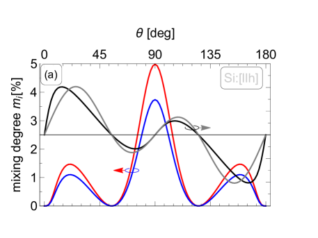
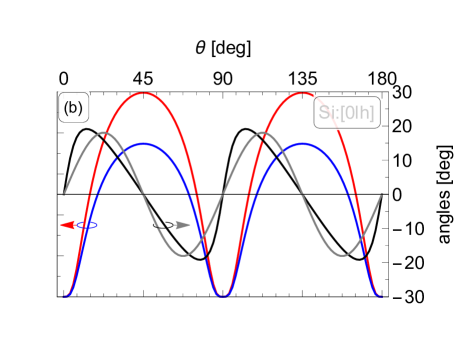
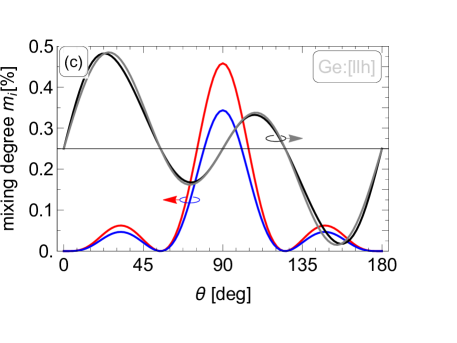
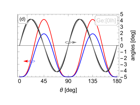
Figure 2: The degree of mixing and the deflection angle for (a) Si:[llh] (b) Si:[0lh] (c) Ge:[llh] (d) Si:[0lh]. The mixing degree given by $m_{1}$ (black) and $m_{2}$ (grey) has the y-axis on the left and the deflection angle [found numerically in red, calculated according to Eq. (17) in blue] has the y-axis on the right. The horizontal axis shows the angle $\theta$, which parametrizes the growth direction orientation as described in Sec. IV.1.

IV.3 Mixing degree

The mixing degree and the deflection angle are plotted in Fig. 2. Starting with the [llh] scenario and Si parameters, Fig. 2a, we observe that as the growth direction changes, the LH-content varies between 0 and 5%, the maximum achieved at $\theta=\pi/2$ corresponding to [110]. The two measures based on the LH-content ($m_{1}$ in red and $m_{2}$ in blue) have very similar shapes but slightly different numerical values. The corresponding deflection angle also varies and reaches values up to $20^{\circ}$ ($\theta_{\scriptscriptstyle+}^{n}$ plotted in black). The analytical result for the approximate spinor (gray) shows that Eq. (17) is a good approximation for finding the closest pure spinor.

We point out that the deflection angle is not specified uniquely by the mixing strength: while both go to zero at high-symmetry growth directions such as [001] and [111], the deflection angle is zero also at [110] where the mixing is maximal. In this case, the Hamiltonian does not contain any deflection-generating terms $\{J_{{x^{\prime}}/{y^{\prime}}},J_{z^{\prime}}\}$, but only the purely mixing term $\{J_{x^{\prime}},J_{y^{\prime}}\}$. Looking at the [0lh] scenario shown in Fig. 2b, one can see that while the curves have different shapes, the overall magnitude of the effects is very similar. Turning next to germanium, plotted in Fig. 2c–d, the curves have shapes very similar to those for silicon, except for the overall magnitude. In Ge, both the mixing and the deflection angle are much smaller. The difference can be traced back to a much stronger dominance of the term $-J_{z^{\prime}}^{2}$ in Ge than in Si (compare the black versus colored lines in Fig. 1).

V The form and strength of the generated SOI

After quantifying the mixing measures $m_{1}$ and $m_{2}$ based on the LH content, we now turn to $m_{3}$, motivated by an important practical question: Assuming that there is Rashba SOI in the bulk, Eq. (10), what is the arising SOI in the heavy-hole subband? Apart from being expected in Si and Ge, the form of Eq. (10) is beneficial due to its rotational symmetry. We will find that the SOI generated in the heavy-hole subband consists of two terms,

$$H_{r}^{\mathrm{\scriptscriptstyle 2D}}=H_{r,\mathrm{def}}^{\mathrm{\scriptscriptstyle 2D}}+H_{r,\mathrm{mix}}^{\mathrm{\scriptscriptstyle 2D}},$$ (18)

induced, respectively, by the coordinate frame deflection and the heavy-hole–light-hole mixing. We next explain the origin of these two terms.

V.1 SOI generated by deflection terms

In the previous section, we have explained that terms in Eq. (15c) can be removed from the Hamiltonian by a suitable coordinate rotation (see App. C). In this rotated frame, the leading-order term in the spinor Hamiltonian is $-J_{z^{\prime\prime}}^{2}$. On the other hand, the electric field $\mathbf{E}$ inducing the bulk Rashba SOI is typically along the growth axis ${z^{\prime}}$. The deflection of these two axes, by angle $\theta_{\scriptscriptstyle+}$, induces SOI in the heavy-hole subband. Indeed, using the pure-hole spinor projection rules Eq. (1) in the deflected coordinate system one has (see App. B)

$$H_{r,\mathrm{def}}^{\mathrm{\scriptscriptstyle 2D}}=\alpha_{r}^{\mathrm{\scriptscriptstyle 3D}}\,\sin\theta_{\scriptscriptstyle+}\,E_{z^{\prime}}\,s_{z^{\prime\prime}}(\mathbf{k}\cdot\mathbf{m}),$$ (19)

where we remind that $\mathbf{m}$ is a unit vector that lies in the ${x^{\prime}}$${y^{\prime}}$ plane and is perpendicular to the plane ${z^{\prime\prime}}$${z^{\prime}}$. We thus conclude that the deflection results in a SOI in the first order of $\theta_{\scriptscriptstyle+}$, in turn in the first order of the rotation-inducing strengths in Eq. (15c). The SOI is of unusual form, the (almost) out-of-plane pseudo-spin operator $s_{z^{\prime\prime}}$. Also, since it contains a single psedo-spin sigma matrix, the SOI field direction does not depend on the momentum direction. Such SOI generates a persistent spin helix [73, 74, 75, 76, 77].

V.2 SOI generated by mixing

Since the Luttinger Hamiltonian is bilinear in spin operators, after removing the rotation-generating terms, there are only two remaining possibilities, given in Eq. (15f). Assuming that such terms are present (or generated by the coordinate rotation in second order in $\gamma_{\delta}$), we are interested in the degree of mixing that they result in. The mixing quantification using measures $m_{1}$ and $m_{2}$ is given in Fig. 2. We now focus on the third measure, proposed in Eq. (12).

To this end, we derive the effective SOI in the heavy-hole subspace that is induced by the bulk Rashba interaction, Eq. (10), and the heavy-hole–light-hole mixing terms in Eq. (15f) denoted as $H_{\mathrm{mix}}$. We assume that both of these terms are small so that we can treat them perturbatively. Using quasi-degenerate perturbation theory, we get the effective Hamiltonian

$$H_{r}^{\mathrm{\scriptscriptstyle 2D}}=P_{\mathrm{hh}}\left(H_{r}^{\mathrm{\scriptscriptstyle 3D}}-\frac{\{H_{r}^{\mathrm{\scriptscriptstyle 3D}},H_{\mathrm{mix}}\}}{\Delta}\right)P_{\mathrm{hh}}+O(H_{\mathrm{mix}}^{2}).$$ (20)

Here, $P_{\mathrm{hh}}$ is the projector to the heavy-hole subspace [equal to $\rho_{\pm 3/2}$ defined below Eq. (8)] and the two terms in the bracket give the zeroth and first-order perturbation in $H_{\mathrm{mix}}$. The first term inside the large brackets in Eq. (20) embodies the pure heavy-hole limit. Relying on the projection rules given in Eq. (1), without any deflection there is no SOI induced in the heavy-hole subspace. A finite deflection generates the expression given in Eq. (19). The second term in the large brackets in Eq. (20) induces finite matrix elements of the in-plane spin operators, as $O(H_{\mathrm{mix}})$ corrections to Eq. (1). The explicit formulas are in Table 1.

		$H_{\mathrm{mix}}$
$H_{r}^{\mathrm{\scriptscriptstyle 3D}}$		none	$\frac{c_{xy}}{2}\{J_{x},J_{y}\}$	$\frac{c_{xx}-c_{yy}}{2}(J_{x}^{2}-J_{y}^{2})$
$J_{x}$	$\,\overset{\mathrm{hh}}{\to}\,$	0	$-\frac{3c_{xy}}{\Delta}\times s_{y}$	$-\frac{3(c_{xx}-c_{yy})}{\Delta}\times s_{x}$
$J_{y}$		0	$\frac{3c_{xy}}{\Delta}\times s_{x}$	$-\frac{3(c_{xx}-c_{yy})}{\Delta}\times s_{y}$
$J_{z}$		$3s_{z}$	0	0

Table 1: Bulk-hole spin to heavy-hole pseudospin projection rules. With heavy-hole–light-hole mixing-inducing terms term(s) $H_{\mathrm{mix}}$ present in the Hamiltonian, the bulk spin operator given in the first column induces finite matrix elements within the heavy-hole subspace, expressed using an effective pseudo-spin operator $\mathbf{s}$ given in the corresponding table entry. The coefficients $c_{ij}$ are the strengths of the terms in $H_{\mathrm{mix}}$, as defined in Eq. (14). The given projections are valid in any coordinate frame where the bulk hole Hamiltonian is $c_{zz}J_{z}^{2}+H_{\mathrm{mix}}$. In the text, this frame is denoted with doubly primed coordinates ${x^{\prime\prime}}$, ${y^{\prime\prime}}$, ${z^{\prime\prime}}$. However, we omit the primes in the table to ease the notation.

The form and strength of the SOI in the heavy-hole subband induced by the bulk Rashba interaction and light-hole–heavy-hole mixing can now be read off from Tab. 1. Assume that only one type of mixing term is present, and start with $H_{\mathrm{mix}}\propto J_{x^{\prime\prime}}^{2}-J_{y^{\prime\prime}}^{2}$. Using the last column of the table, one sees that the projection preserves the bulk SOI form with a renormalized strength

$$H_{r,\mathrm{mix}}^{\mathrm{\scriptscriptstyle 2D}}=-3\frac{c_{{x^{\prime\prime}}{x^{\prime\prime}}}-c_{{y^{\prime\prime}}{y^{\prime\prime}}}}{\Delta}E_{z^{\prime}}(s_{x^{\prime\prime}}k_{y^{\prime}}-s_{y^{\prime\prime}}k_{x^{\prime}}).$$ (21)

For the other mixing term, $H_{\mathrm{mix}}\propto\{J_{x^{\prime\prime}},J_{y^{\prime\prime}}\}$, the table middle column gives

$$H_{r,\mathrm{mix}}^{\mathrm{\scriptscriptstyle 2D}}=-3\frac{c_{{x^{\prime\prime}}{y^{\prime\prime}}}}{\Delta}E_{z^{\prime}}(s_{x^{\prime\prime}}k_{x^{\prime}}+s_{y^{\prime\prime}}k_{y^{\prime}}).$$ (22)

While this form looks nonstandard, it is unitarily equivalent to Eq. (21) upon rotating the pseudospin axes by $-\pi/2$ around ${z^{\prime\prime}}$. When both mixing terms are present, their action in inducing terms in the effective Hamiltonian is additive, as follows from Eq. (20). The resulting interaction is a sum of the terms in Eq. (21) and Eq. (22). Due to the $-\pi/2$ rotation in the second equation, the two SOI fields are orthogonal and adding them will result in an interaction that is unitarily equivalent to the standard Rashba SOI

$$H_{r,\mathrm{mix}}^{\mathrm{\scriptscriptstyle 2D}}=-m_{3}\times U_{\varphi}\alpha^{\mathrm{\scriptscriptstyle 3D}}E_{z^{\prime}}(s_{x^{\prime\prime}}k_{y^{\prime}}-s_{y^{\prime\prime}}k_{x^{\prime}})U_{\varphi}^{\dagger},$$ (23)

with the pseudospin rotation dependent on the strengths of the mixing terms,

$$U_{\varphi} =\exp(-is_{z^{\prime\prime}}\varphi),$$ (24a)

$$\frac{\sin\varphi}{\cos\varphi} =\frac{c_{{x^{\prime\prime}}{y^{\prime\prime}}}}{c_{{x^{\prime\prime}}{x^{\prime\prime}}}-c_{{y^{\prime\prime}}{y^{\prime\prime}}}},$$ (24b)

and the strength-renormalization

$$|m_{3}|=3\frac{\sqrt{(c_{{x^{\prime\prime}}{x^{\prime\prime}}}-c_{{y^{\prime\prime}}{y^{\prime\prime}}})^{2}+c_{{x^{\prime\prime}}{y^{\prime\prime}}}^{2}}}{\Delta}.$$ (25)

The last equation, the strength of the induced Rashba SOI in the heavy-hole subband appearing upon mixing, is the main result of this section. In a simple expression, it embodies the third measure for the heavy-hole–light-hole mixing as it has been introduced in Eq. (12).

We plot $m_{3}$ in Fig. 3. Black curves show Eq. (12) with the coefficients $c_{i^{\prime\prime}j^{\prime\prime}}$ evaluated exactly, corresponding to a rotated frame where $H_{\mathrm{rot}}$ is exactly zero. The formulas are, again, unwieldy, and we do not give them explicitly. Instead, we provide simplified ones, based on replacing $c_{i^{\prime\prime}j^{\prime\prime}}\to c_{i^{\prime}j^{\prime}}$ and reading off the latter coefficients from Eq. (14):

$$\mathrm{for\,[llh]:}\quad|m_{3}|=\frac{2\gamma_{\delta}\sin^{2}\theta(3\cos 2\theta+1)}{\Delta},$$ (26a)

$$\mathrm{for\,[0lh]:}\quad|m_{3}|=\frac{\gamma_{\delta}\sin^{2}(2\theta)}{\Delta},$$ (26b)

and in both scenarios we take $\Delta\approx 4\overline{\gamma}$. The corresponding $m_{3}$ is plotted in blue in Fig. 3. Again, the leading-order approximations are excellent for Ge, while somewhat larger discrepancies are visible for Si.

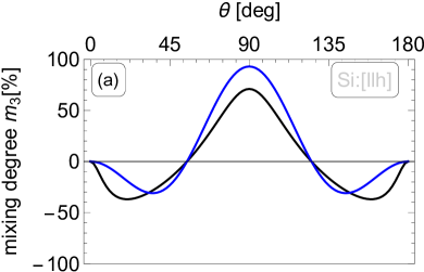
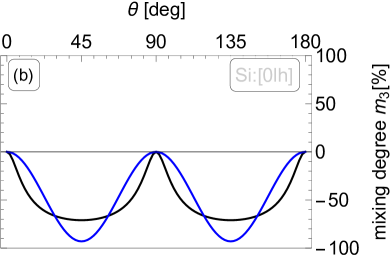
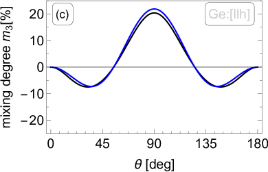
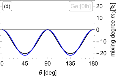
Figure 3: Generated SOI strength. The mixing strength $m_{3}$ for Si (upper row) and Ge (bottom row) for [llh] (left column) and [0lh] (right column). The black curves give Eq. (25) evaluated from the coefficients $c_{ij}$ in the doubly-primed coordinate system ${x^{\prime\prime}}$${y^{\prime\prime}}$${z^{\prime\prime}}$. The blue curves show the approximation in Eq. (26), given by evaluating Eq. (24) using the coefficients $c_{ij}$ from the singly-primed coordinate system ${x^{\prime}}$${y^{\prime}}$${z^{\prime}}$.

VI Applications

Our results allow for a qualitative understanding of the spin structure of holes in quasi-two-dimensional confinement and structures derived from it, such as split-gate QPC or planar quantum dots. We demonstrate the applications of the results with two examples. First, we look at the effective Hamiltonian that describes a heavy hole spin in a finite magnetic field and analyze the associated $g$ tensor. Second, we consider the effects of strain and its gradients.

VI.1 Zeeman interaction and $g$ tensor

We now consider the case where a magnetic field $\mathbf{B}$ is applied. We ignore the orbital effects and neglect the small cubic Zeeman term. The corresponding bulk Hamiltonian is

$$H_{z}^{\mathrm{\scriptscriptstyle 3D}}=2\mu_{B}\kappa\mathbf{B}\cdot\mathbf{J},$$ (27)

where $\mu_{B}$ is the Bohr magneton, $\kappa$ is the $g$ factor. The bulk interaction induces an effective Hamiltonian within the heavy-hole subspace. We can get it from Eq. (20) replacing $H_{r}^{\mathrm{\scriptscriptstyle 3D}}\to H_{z}^{\mathrm{\scriptscriptstyle 3D}}$. Together with Tab. 1, one immediately gets

$$H_{z}^{\mathrm{\scriptscriptstyle 2D}}=\mu_{B}\mathbf{B}\cdot\mathbf{g}U_{\varphi}\mathbf{s}U^{\dagger}_{\varphi},$$ (28)

where $U_{\varphi}$ is defined in Eq. (24) and $\mathbf{g}$ is the $g$ tensor. Applying Tab. 1 means we have derived the preceding equation in the doubly coordinate system. Here, the $g$ tensor is diagonal with the following components

$$\mathbf{g}|_{{x^{\prime\prime}}{y^{\prime\prime}}{z^{\prime\prime}}}=\mathrm{diag}(2\kappa\,m_{3},2\kappa\,m_{3},6\kappa).$$ (29)

In this convenient coordinate system, the effects of the heavy-hole–light-hole mixing on the $g$ tensor are simple. At zero mixing, the $g$-tensor components in the ${x^{\prime\prime}}{y^{\prime\prime}}$ plane are zero. Nonzero mixing induces nonzero and isotropic $g$ tensor in this plane. This simplicity is obscured by the fact that this plane normal is rotated with respect to the growth direction. The $g$ tensor in the other two coordinate systems is

$$\mathbf{g}|_{{x^{\prime}}{y^{\prime}}{z^{\prime}}} =R[\phi,\theta_{\scriptscriptstyle+},-\phi]\,\,\mathbf{g}|_{{x^{\prime\prime}}{y^{\prime\prime}}{z^{\prime\prime}}}\,\,R[\phi,\theta_{\scriptscriptstyle+},-\phi]^{T},$$ (30a)

$$\mathbf{g}|_{{x}{y}{z}} =R[\phi,\theta,-\phi]\,\,\mathbf{g}|_{{x^{\prime}}{y^{\prime}}{z^{\prime}}}\,\,R[\phi,\theta,-\phi]^{T},$$ (30b)

with $\phi=\pi/4$ for [llh] and $\phi=\pi/2$ for [0lh].

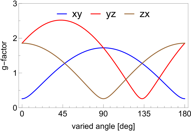
Figure 4: $\bm{g}$ factor as a function of the magnetic field direction $\mathbf{B}=B(\cos\alpha\sin\beta,\sin\alpha\sin\beta,\cos\beta)$ varied over a semicircle in three orthogonal planes as denoted by the legend: ${x^{\prime}}{y^{\prime}}$ means $\beta=\pi/2$ and $\alpha$ is varied, ${y^{\prime}}{z^{\prime}}$ means $\alpha=0$ and $\beta$ is varied, and ${z^{\prime}}{x^{\prime}}$ means $\alpha=\pi/2$ and $\beta$ is varied. The varied angle is on the horizontal axis of the figure. We took the parameters for Si, scenario $[0lh]$ with $\theta=30^{\circ}$, and evaluated the $g$ factor as $g=|\mathbf{B}^{T}\mathbf{g}|/B$ using Eq. (17), (29), and (30).

As an illustration, we plot the $g$ factor, defined as the norm of the vector $\mathbf{B}^{T}\mathbf{g}/B$, calculated using Eq. (29), (30) and the simplified expression for the $m_{3}$, Eq. (17), in Fig. 4. We find it remarkable that our simple model shows $g$ factor dependences qualitatively similar to those observed experimentally in an MOS Si quantum dot as well as in much more elaborate simulations [24].

VI.2 Spin qubit: dephasing and Rabi driving

The $g$ tensor derived in the previous section can be used to analyze a spin qubit realized by a heavy hole. We start by rewriting Eq. (28) as

$$H_{q}=\mu_{B}[R_{\varphi}(\mathbf{B}^{T}\mathbf{g})]\cdot\mathbf{s}\equiv\mu_{B}\mathbf{B}_{q}\cdot\mathbf{s},$$ (31)

where $R_{\varphi}$ induces the same rotation (around ${z^{\prime\prime}}$ by angle $\varphi$) on a three-dimensional vectors as $U_{\varphi}$ induces on spinors. We have also introduced the effective magnetic field $\mathbf{B}_{q}$ coupled to the pseudo-spin $\mathbf{s}$.

Several standard performance metrics, including the qubit dephasing, lifetime, or Rabi frequency, can be extracted from the effective spin qubit Hamiltonian in Eq. (31). They follow from its dependence on electric and magnetic fields, either controlled or fluctuating due to noise. We will not go into quantitative details since our model omits details of the quantum dot confinement. However, we can use Eq. (31) to elucidate the physical origins of some of these effects. To this end, we emulate confinement changes as changes of the parameter $\theta$. While we introduced it as a sample growth direction, we now reinterpret it as an effective confinement direction that can be changed. For example, pulling the confined hole against the side or the top of a finFET or an MOS structure or moving it with respect to a nearby charge impurity could be perceived as tilting the effective confinement plane.

With this interpretation, we can start with the examination of ‘sweet spots’, being the directions of the magnetic field $\mathbf{B}$ where the $g$ factor achieves its extremum with respect to the variations in $\theta$. Since $\theta$ is an angle, the $g$ factor curve must be periodic in it and there will be at least two sweet spots (in $\theta$) for any $\mathbf{B}$. Translating into equations, one would look for solutions of the following requirement:

$$\mathrm{maximal\,T_{2}^{*}}:\quad\min_{\mathbf{B}}|\mathbf{B}_{q}\cdot\partial_{\theta}\mathbf{B}_{q}|.$$ (32a)

Similarly, the qubit relaxation is mediated through the transverse matrix element of the effective magnetic field,

$$\mathrm{maximal\,T_{1}}:\quad\min_{\mathbf{B}}|\mathbf{B}_{q}\times\partial_{\theta}\mathbf{B}_{q}|.$$ (32b)

However, since usually the relaxation is slow and not of concern, instead of minimizing this matrix element to minimize the relaxation rate, one is interested in finding its maximum, as the same matrix element mediates qubit Rabi rotations under resonant excitation. However, to describe such a situation, one needs to include the effects which originate in the time-dependence of the frame in which the effective Hamiltonians, Eqs. (20), (23), (28), were derived. As we show in App. C, the time dependence generates an additional effective time-dependent magnetic field

$$\mathbf{B}_{U}=\mathbf{m}\frac{\hbar}{2\kappa\mu_{B}}\partial_{t}(\theta+\theta_{\scriptscriptstyle+}).$$ (32c)

Upon adding $\mathbf{B}_{U}$ to $\mathbf{B}_{q}$, one can, for example, search for the maximum of the right-hand side of Eq. (32b). As stated, we could straightforwardly plot any of these matrix elements in the same way as the $g$ factor in Fig. 4 and examine the extrema. However, since there have been several recent works that do such an analysis [25, 81, 82, 30], instead of repeating it, we comment on the sources of Rabi oscillations appearing in our model.

We consider that an oscillating gate potential induces small oscillations in the effective confinement direction $\theta$. The corresponding time-dependent effective Hamiltonian is

$$H_{q}=\mu_{B}\mathbf{B}\cdot\mathbf{g}U_{\varphi}\mathbf{s}U^{\dagger}_{\varphi}+\mathbf{m}\hbar\partial_{t}(\theta+\theta_{\scriptscriptstyle+}).$$ (33)

Varying $\theta$ will induce 1) changes of the $g$ tensor ‘in-plane’ components through changing the value of $m_{3}$, 2) changes of the value of the angle $\varphi$ defining the ‘in-plane’ axes in the pseudo-spin space, and 3) a fictitious magnetic field $\mathbf{B}_{U}$ due to the time-dependent frame rotation. To draw analogies to the existing results for holes and electrons, we note that with the magnetic field applied perpendicular to the confinement axis ${z^{\prime}}$, the arising Hamiltonian terms are longitudinal (approximately, neglecting here the deflection angle $\theta_{\scriptscriptstyle+}$) in 1) and transverse in 2) and 3). The latter two channels will, therefore, be more efficient in inducing Rabi oscillations. Loosely speaking, the channel 1) corresponds to the modulation of the $g$-tensor eigenvalues and 2) and 3) its eigenvectors (‘iso-Zeeman’ in the nomenclature of Ref. [17]). We point out that the Rabi oscillations associated with $H_{q}$ do not rely on the SOI terms in Eq. (18). Adding them to the effective Hamiltonian and promoting the in-plane momenta to $c$-numbers oscillating in time, 4) an additional channel to induce Rabi oscillation arises. Since the linear-in-momenta SOI terms can be viewed, in the lowest order of the dot size over the SOI length, as a gauge transformation, this channel is similar in spirit to the fictitious magnetic field $\mathbf{B}_{U}$ induced by the time-dependent frame. In a given device all four channels will interfere in inducing Rabi oscillations.

VI.3 Strain and SOI

We now look at strain, as it profoundly affects holes [83, 51, 2, 20]. The strain in the device is parametrized by a symmetric strain tensor $\epsilon_{ij}$. Its elements generate additional terms in the bulk hole Hamiltonian [83],

$$\begin{split}H_{BP}=&-\frac{2}{3}D_{u}\left(\epsilon_{xx}J_{x}^{2}+\mathrm{c.p.}\right)\\ &-\frac{2}{3}D_{u}^{\prime}(\epsilon_{xy}\{J_{x},J_{y}\}+\mathrm{c.p.}),\end{split}$$ (34)

where the deformation potentials $D_{u}$ and $D_{u}^{\prime}$ are material parameters. Different to previous sections, we do not consider rotations of the ‘growth direction’, which would here correspond to rotations of the strain tensor. We assume a fixed growth direction [001] and consider in-plane strain $\epsilon_{xx}=\epsilon_{yy}=\epsilon_{||}<0$, relevant, for example, for lattice-matched heterostructures. The inplane compression induces out-of-plane expansion $\epsilon_{zz}=-2\epsilon_{||}c_{12}/c_{11}$, with material-dependent elastic constants $c_{11}$ and $c_{12}$. Inserting this form of the diagonal strain tensor components into Eq. (34), we get (constant omitted)

$$\begin{split}H_{BP}=&-\frac{2}{3}D_{u}J_{z}^{2}\left(\epsilon_{zz}-\epsilon_{||}\right)\\ &-\frac{2}{3}D_{u}^{\prime}(\epsilon_{xy}\{J_{x},J_{y}\}+\epsilon_{yz}\{J_{y},J_{z}\}+\epsilon_{zx}\{J_{z},J_{x}\}).\end{split}$$ (35)

The Hamiltonian is analogous to Eq. (14). The term in the first line sets the unperturbed system with the pure spinors given in Eq. (5) as its eigenstates and providing for the heavy-hole–light-hole splitting,

$$\Delta=\frac{4}{3}D_{u}\left(\epsilon_{zz}-\epsilon_{||}\right).$$ (36)

The second line of Eq. (35) contains the perturbing terms. Classifying them using Eq. (15), the last two terms induce deflection of the spinor axis away from the growth direction, here equal to the crystal axis ${z^{\prime}}={z}$. In analogy to Eq. (17), these off-diagonal strain components, quantified by $\epsilon_{\mathrm{rot}}^{2}=\epsilon_{zx}^{2}+\epsilon_{yz}^{2}$, generate a deflection angle

$$\sin\theta_{\scriptscriptstyle+}=\frac{D_{u}^{\prime}}{D_{u}}\frac{\epsilon_{\mathrm{rot}}}{\epsilon_{zz}-\epsilon_{||}}.$$ (37)

Neglecting the small contribution from this deflection, the heavy-hole–light-hole mixing is given by the first term in the second line of Eq. (35),

$$c_{{x^{\prime\prime}}{y^{\prime\prime}}}\approx c_{{x^{\prime}}{y^{\prime}}}=c_{{x}{y}}=-\frac{4}{3}D_{u}^{\prime}\epsilon_{xy}.$$ (38)

Using Eq. (36), we can evaluate Eq. (12),

$$m_{3}=3\frac{D_{u}^{\prime}}{D_{u}}\frac{\epsilon_{xy}}{\epsilon_{zz}-\epsilon_{||}}.$$ (39)

The two quantities characterizing the perturbing terms, the mixing $m_{3}$ and the deflection angle $\theta_{\scriptscriptstyle+}$, are plotted in Fig. 5. Once again, one can see a substantial SOI (measured by $m_{3}$; the left $y$ axis) arises already at relatively small strains. It is generated primarily by the in-plane off-diagonal strain components $\epsilon_{xy}$. With strains as small as a few times $10^{-4}$ (expected in typical devices [84]), the SOI generated in the heavy-hole subband has strength comparable to its value in the bulk ($m_{3}$ of order 1). The off-diagonal out-of-plane strain tensor elements, on the other hand, induce primarily a deflection of the pure spinor direction. The values denoted on the right $y$ axis convert $m_{3}$ to the corresponding deflection angle $\theta_{\scriptscriptstyle+}$. In the range plotted, the right-hand side of Eq. (37) is small, the deflection angle $\theta_{\scriptscriptstyle+}$ is linear in the off-diagonal strain components, and the two quantities are proportional.

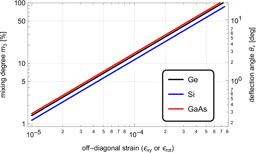
Figure 5: Strain-generated mixing and deflection angle. Referring to the left $y$ axis and the parameter $\epsilon_{xy}$ on the horizontal axis, the curves show Eq. (39), the mixing measure $m_{3}$. Referring to the right $y$ axis and the parameter $\epsilon_{\mathrm{rot}}$ on the horizontal axis, the same curves show Eq. (37), the deflection angle $\theta_{\scriptscriptstyle+}$. We use $\epsilon_{||}=-0.61\%$, inspired by values appropriate for $\mathrm{Ge/Ge_{0.8}Si_{0.2}}$ heterostructures [59].

VI.4 Strain gradients and Rabi driving

Elaborate numerical and analytical analysis of Ref. [58] considered strain-gradients, which together with periodically displacing a Ge quantum-dot hole in space induce Rabi oscillations. It was found that strain components $\epsilon_{xz}$ and $\epsilon_{yz}$ are most effective in inducing Rabi oscillations. We can provide a simple explanation based on our analysis. According to Eq. (35), the associated spin operators belong to $H_{\mathrm{rot}}$ in Eq (15). Such operators lead, predominantly, to a rotation of the heavy-hole spinor (a ‘deflection’ in our nomenclature). The corresponding rotation of the reference frame (see App. C) induces Rabi oscillations through the last term in Eq. (33), which is linear in $\partial_{t}\theta_{\scriptscriptstyle+}$, in turn linear in $\epsilon_{\mathrm{rot}}$ according to Eq. (37). The requirement for resonance means the frequency of driving equals the Zeeman energy $|\mu_{B}\mathbf{B}_{q}|.$ On the other hand, the term $\epsilon_{xy}\{J_{x},J_{y}\}$ belongs to $H_{\mathrm{mix}}$, meaning $\theta_{\scriptscriptstyle+}\approx 0$, and enters into Eq. (33) in the second order, the second term in the bracket in Eq. (20). Its contribution to Rabi driving is thus expected to be smaller.

VII Conclusions

We have analyzed the heavy-hole–light-hole mixing in quasi-two-dimensional semiconductors. This mixing is central to many spin effects in devices based on holes in quasi-two-dimensional structures. Particularly, it is responsible for the response of the hole spin to electric fields. We have suggested several measures of the mixing and quantified the relations between them. We find that the measures based on the light-hole content in the wave function somewhat underestimate the efficiency of mixing in inducing the SOI: with a light-hole content that might be considered ‘small’, the arising SOI is essentially of the same strength as the one in the bulk.

We have adopted the zone-center approximation, which amounts to neglecting the in-plane momenta $k_{x}=0=k_{y}$. The approximation allows one to derive analytical results and get physical insight into various aspects of heavy-hole spin. Within this calculation scheme, we could identify different types of terms in the hole kinetic energy and strain Hamiltonians. Terms of the first type induce a rotation of the direction of spinors while keeping them pure. These terms are most efficient in inducing Rabi oscillations, acting analogously to Rashba or Dresselhaus SOIs inducing Rabi rotations in the conduction band through the EDSR. They also preserve the $g$-tensor eigenvalues. Terms of the second type admix the light-hole components. They are less efficient for Rabi driving and more profoundly change the $g$-tensor. They are responsible for the $g$-tensor finite in-plane components.

The zone-center description provides a simple analytical model with which the basic characteristics of a spin qubit can be investigated without any sophisticated numerics or simulations. We have exemplified it by plotting the hole g-factor and gave formulas from which matrix elements responsible for hole spin dephasing, relaxation, or Rabi frequency can be obtained straightforwardly. An interesting extension of our work would be to include the in-plane orbital degrees of freedom perturbatively and analyze to which extent the simple scheme presented here can be used semi-quantitatively. We leave the establishment of such a connection to elaborate numerical models for the future.

Appendix A Derivation of Tab. 1

Expressing the mixing terms through operators $J_{\pm}$ defined in Footnote 17, it is straightforward to derive the following table

 J+→{.,Hmix}2J+3/i2J+3 J−2J−3.fragments fragments fragments J→{.,Hmix}fragments2J3ifragments2J3fragments Jfragments2J3ifragments2J3\begin{tabular}[]{@{\quad}c@{\quad}c@{\quad}c@{\quad}c@{}}\hline\cr\hline\cr&&\lx@intercol\hfil$H_{\mathrm{mix}}$\hfil\lx@intercol\\ \cline{3-4}\cr$H_{r}^{\mathrm{\scriptscriptstyle 3D}}$&&$\{J_{x},J_{y}\}$&$J_{x}^{2}-J_{y}^{2}$\\ \hline\cr$J_{+}$&\hbox{\multirowsetup$\overset{\{.,H_{\mathrm{mix}}\}}{\xrightarrow{\hskip 28.45274pt}}$}&$2J_{+}^{3}/i$&$2J_{+}^{3}$\\ $J_{-}$&&$-2J_{-}^{3}/i$&$2J_{-}^{3}$\\ \hline\cr\hline\cr\end{tabular}.

Hmix   Hr3D {Jx,Jy}-Jx2Jy2Hmix   Hr3D {Jx,Jy}-Jx2Jy2 (40)

The body of the table gives the anticommutator $\{H_{r}^{\mathrm{\scriptscriptstyle 3D}},H_{\mathrm{mix}}\}$, dropping the terms that are zero upon projecting them to the heavy-hole subspace by $P_{\mathrm{hh}}\cdot P_{\mathrm{hh}}$, for two alternatives for $H_{\mathrm{mix}}$ and two alternatives for $H_{r}^{\mathrm{\scriptscriptstyle 3D}}$ as given in the table row and column headers. Evaluating a single matrix element $\langle\Psi_{3/2}^{\mathrm{pure}}|J_{+}^{3}|\Psi_{-3/2}^{\mathrm{pure}}\rangle=3/\sqrt{2}$, the remaining matrix elements being zero, we get

$$J_{\pm}^{3}\raisebox{-1.0pt}[0.0pt][0.0pt]{$\,\overset{\mathrm{hh}}{\to}\,$}P_{\mathrm{hh}}J_{\pm}^{3}P_{\mathrm{hh}}=3s_{\pm}.$$ (41)

With this, the table for projections becomes

 J+→Phh{.,Hmix}Phh6s+/i6s+ J−6s−.fragments fragments fragments J→Phh{.,Hmix}Phhfragments6sifragments6sfragments Jfragments6sifragments6s\begin{tabular}[]{@{\quad}c@{\quad}c@{\quad}c@{\quad}c@{}}\hline\cr\hline\cr&&\lx@intercol\hfil$H_{\mathrm{mix}}$\hfil\lx@intercol\\ \cline{3-4}\cr$H_{r}$&&$\{J_{x},J_{y}\}$&$J_{x}^{2}-J_{y}^{2}$\\ \hline\cr$J_{+}$&\hbox{\multirowsetup$\overset{P_{\mathrm{hh}}\{.,H_{\mathrm{mix}}\}P_{\mathrm{hh}}}{\xrightarrow{\hskip 28.45274pt}}$}&$6s_{+}/i$&$6s_{+}$\\ $J_{-}$&&$-6s_{-}/i$&$6s_{-}$\\ \hline\cr\hline\cr\end{tabular}.

Hmix   Hr {Jx,Jy}-Jx2Jy2Hmix   Hr {Jx,Jy}-Jx2Jy2 (42)

To get Tab. 1 in the main text, each entry should be multiplied by $-1/\Delta$ and the rows should be linearly combined to switch back to the Cartesian-index operators $J_{x}$ and $J_{y}$.

Appendix B Derivations of the SOI projections

Here we show how to derive results such as Eqs. (19), (21), and (22) using the projection rules given in Tab. 1. The rules (for going from the bulk spin operators $\mathbf{J}$ to heavy-hole pseudospin operators $\mathbf{s}$) are simple in the deflected coordinate frame ${x^{\prime\prime}}$–${y^{\prime\prime}}$–${z^{\prime\prime}}$. However, in going from the bulk to the two-dimensional hole gas, we are implicitly applying further ‘rules’ for the momentum operators, namely $k_{z^{\prime}}\raisebox{-1.0pt}[0.0pt][0.0pt]{$\,\overset{\scriptscriptstyle 2D}{\to}\,$}0$. One can also understand the fact that the electric field is along the growth direction as yet another rule, $E_{x^{\prime}}\raisebox{-1.0pt}[0.0pt][0.0pt]{$\,\overset{\scriptscriptstyle 2D}{\to}\,$}0$ and $E_{y^{\prime}}\raisebox{-1.0pt}[0.0pt][0.0pt]{$\,\overset{\scriptscriptstyle 2D}{\to}\,$}0$. Therefore, the projection for the spin operators and for the momentum and electric field vectors are simplest in different coordinate frames. The relative rotation between these two reference frames needs to be taken into account and will complicate the resulting expressions, in principle. However, here we show that the resulting differences are of order $O(\theta_{+}^{2})=O(\gamma_{d}^{2})$ and can be thus neglected within the precision that we work with, set by the perturbation order included in Eq. (20).

To show it, we first note that the relative rotation between the singly- and doubly-primed coordinates is given by Eq. (13b) with $\theta\to\theta_{\scriptscriptstyle+}$ and the angles $\phi^{\prime}=-\phi$ as specified for the two scenarios. This simplification is due to the choice $\phi^{\prime}=-\phi$. The elements of matrix $R$ then give overlaps between axes directions in the two coordinate frames. We note that ${\mathbf{x}^{\prime\prime}}\cdot{\mathbf{x}^{\prime}}=1+O(\theta_{\scriptscriptstyle+}^{2})$, the same for the alignment of the $y$ axes, and ${\mathbf{x}^{\prime\prime}}\cdot{\mathbf{y}^{\prime}}=O(\theta_{\scriptscriptstyle+}^{2})$. Therefore, to precision $O(\theta_{\scriptscriptstyle+}^{2})$, the axes $x$ and $y$ are aligned in both coordinate systems.

We now turn to Eq. (19). Starting with the bulk Rashba SOI, Eq. (10), stripped of the overall constant, we apply the leading-order (Tab. 1 for $H_{\mathrm{mix}}=\mathrm{none}$) projection rule for the spin operators in the doubly primed coordinate system:

$$\mathbf{J}\cdot(\mathbf{k}\times\mathbf{E})\raisebox{-1.0pt}[0.0pt][0.0pt]{$\,\overset{\mathrm{hh}}{\to}\,$}s_{z^{\prime\prime}}{\mathbf{z}^{\prime\prime}}\cdot(\mathbf{k}\times\mathbf{E}).$$ (43)

Next, we use the cyclic property of the cross product

$$s_{z^{\prime\prime}}\mathbf{k}\cdot(\mathbf{E}\times{\mathbf{z}^{\prime\prime}}),$$ (44)

and use the ‘rule’ for the electric field vector to get

$$E_{z^{\prime}}s_{z^{\prime\prime}}\mathbf{k}\cdot({\mathbf{z}^{\prime}}\times{\mathbf{z}^{\prime\prime}}).$$ (45)

As the angle between the $z$ axes in the two coordinate systems is $\theta_{\scriptscriptstyle+}$, we arrive at Eq. (19).

We now retrace these steps for the first-order corrections. Let us consider the mixing term $J_{x^{\prime\prime}}^{2}-J_{y^{\prime\prime}}^{2}$, corresponding to the last column of Tab. 1 and omit the numerical factor $-3(c_{{x^{\prime\prime}}{x^{\prime\prime}}}-c_{{y^{\prime\prime}}{y^{\prime\prime}}})/\Delta$, so that the projection rule is $J_{x^{\prime\prime}}\raisebox{-1.0pt}[0.0pt][0.0pt]{$\,\overset{\mathrm{hh}}{\to}\,$}s_{x^{\prime\prime}}$, $J_{y^{\prime\prime}}\raisebox{-1.0pt}[0.0pt][0.0pt]{$\,\overset{\mathrm{hh}}{\to}\,$}s_{y^{\prime\prime}}$, $J_{z^{\prime\prime}}\raisebox{-1.0pt}[0.0pt][0.0pt]{$\,\overset{\mathrm{hh}}{\to}\,$}0$. We have

$$\mathbf{J}\cdot(\mathbf{k}\times\mathbf{E})\raisebox{-1.0pt}[0.0pt][0.0pt]{$\,\overset{\mathrm{hh}}{\to}\,$}(s_{x^{\prime\prime}}{\mathbf{x}^{\prime\prime}}+s_{y^{\prime\prime}}{\mathbf{y}^{\prime\prime}})\cdot E_{z^{\prime}}(k_{y^{\prime}}{\mathbf{x}^{\prime}}-k_{x^{\prime}}{\mathbf{y}^{\prime}}),$$ (46)

where to get the second bracket, we used that $\mathbf{E}=E_{z^{\prime}}{\mathbf{z}^{\prime}}$. Neglecting the $O(\theta_{\scriptscriptstyle+}^{2})$ terms in the dot products of the axes vectors of the two coordinate frames, we get

$$E_{z^{\prime}}(s_{x^{\prime\prime}}k_{y^{\prime}}-s_{y^{\prime\prime}}k_{x^{\prime}}),$$ (47)

which is Eq. (21). With the other mixing term, the result in Eq. (22) follows analogously.

Appendix C Time-dependent effective growth direction

Here we elucidate the effective heavy-hole Hamiltonian describing the system when the angle $\theta$ is time dependent. In such a case, the angle should be interpreted as an effective confinement direction, that is, the normal of a surface against which the confinement presses the hole. Apart from the heterostructure, the gates and environmental electric noise also contribute to the confinement potential. Considering the time-dependent value of $\theta$ is then reasonable, though its changes will typically be small.

Before generalizing to a time-dependent case, we summarize the derivation presented in the main text for constant $\theta$. We start with a band center Hamiltonian,

$$H=H_{0}(\mathbf{J},\mathbf{J})+H_{\mathrm{rot}}(\mathbf{J},\mathbf{J})+H_{\mathrm{mix}}(\mathbf{J},\mathbf{J})+H^{\scriptscriptstyle 3D}(\mathbf{J}\cdot\mathbf{A}).$$ (48)

With the last term, we include a generic bulk Hamiltonian with an unspecified vector $\mathbf{A}$, covering both the SOI and Zeeman terms considered in the main text. The arguments in brackets denote that the first three terms are quadratic, and the last term is linear in the spin operators $\mathbf{J}$. The terms are defined in Eqs. (14) and classified into parts in Eq. (15). We have also used $H_{0}(\mathbf{J},\mathbf{J})=-(\Delta/2)(\mathbf{J}\cdot\mathbf{{z^{\prime}}})^{2}$.

We write the quadratic terms as three-by-three matrices $M$,

$$H={\mathbf{J}^{\prime}}\cdot\left({M_{0}^{\prime}}+{M_{\mathrm{rot}}^{\prime}}+{M_{\mathrm{mix}}^{\prime}}\right){\mathbf{J}^{\prime}}+H^{\scriptscriptstyle 3D}({\mathbf{J}^{\prime}}\cdot{\mathbf{A}^{\prime}}),$$ (49)

and note that their elements, if taken from Eq. (14), correspond to the coordinate system ${x^{\prime}}$–${y^{\prime}}$–${z^{\prime}}$. We have denoted this using a prime on all quantities. Our central point in the main text was that upon finding a suitable direction parameterized by ${z^{\prime\prime}}$, the bilinear terms can be written with the form given in the previous equation with ${M_{\mathrm{rot}}^{\prime\prime}}=0$,

$$H={\mathbf{J}^{\prime\prime}}\cdot\left({M_{0}^{\prime\prime}}+{M_{\mathrm{mix}}^{\prime\prime}}\right){\mathbf{J}^{\prime\prime}}+H^{\scriptscriptstyle 3D}({\mathbf{J}^{\prime}}\cdot{\mathbf{A}^{\prime}}),$$ (50)

where the elements of $M$ matrices might have changed values, but their form (which elements are zero) is fixed by the definition in Eq. (15). Particularly, ${M_{0}^{\prime\prime}}$ is still a matrix with a single nonzero element, corresponding to a projector $|{z^{\prime\prime}}\rangle\langle{z^{\prime\prime}}|$. The transformation from Eq. (49) to (50) is a change of the basis of the three-dimensional space, that is, a rotation. We make this rotation explicit,

$$H={\mathbf{J}^{\prime}}\cdot R_{\theta_{\scriptscriptstyle+}}\left({M_{0}^{\prime\prime}}+{M_{\mathrm{mix}}^{\prime\prime}}\right)R_{\theta_{\scriptscriptstyle+}}^{T}{\mathbf{J}^{\prime}}+H^{\scriptscriptstyle 3D}({\mathbf{J}^{\prime}}\cdot{\mathbf{A}^{\prime}}),$$ (51)

with $R_{\theta_{\scriptscriptstyle+}}^{T}$ being the rotation taking the axis ${z^{\prime}}$ to ${z^{\prime\prime}}$, that is $R_{\theta_{\scriptscriptstyle+}}=R[\phi,\theta_{\scriptscriptstyle+},-\phi]$ given in Eq. (13).

We now trade the three-component vector rotation for a corresponding (with the same Euler angles) spinor rotation $U_{\theta_{\scriptscriptstyle+}}$, using the identity $U\mathbf{J}U^{\dagger}=R^{T}\mathbf{J}$ for a corresponding rotation pair $R\leftrightarrow U$,

$$H=U_{\theta_{\scriptscriptstyle+}}\left[{\mathbf{J}^{\prime}}\cdot\left({M_{0}^{\prime\prime}}+{M_{\mathrm{mix}}^{\prime\prime}}\right){\mathbf{J}^{\prime}}\right]U_{\theta_{\scriptscriptstyle+}}^{\dagger}+H^{\scriptscriptstyle 3D}({\mathbf{J}^{\prime}}\cdot{\mathbf{A}^{\prime}}).$$ (52)

Next, we move the last term inside the unitaries,

$$H=U_{\theta_{\scriptscriptstyle+}}\left[{\mathbf{J}^{\prime}}\cdot\left({M_{0}^{\prime\prime}}+{M_{\mathrm{mix}}^{\prime\prime}}\right){\mathbf{J}^{\prime}}+H^{\scriptscriptstyle 3D}({\mathbf{J}^{\prime}}\cdot{\mathbf{A}^{\prime\prime}})\right]U_{\theta_{\scriptscriptstyle+}}^{\dagger},$$ (53)

where we used $R^{T}_{\theta_{\scriptscriptstyle+}}{\mathbf{A}^{\prime}}={\mathbf{A}^{\prime\prime}}$. This Hamiltonian makes explicit the frame that has been implicit in the derivations in the main text. As the final step towards an effective Hamiltonian valid for a time-dependent frame, we switch to a time-independent frame for the spin operator. We choose the crystallographic coordinates for such a frame, even though doubly-primed axes corresponding to an arbitrary fixed value of $\theta_{0}$ would be equally suitable. In analogy with the above, it results in the replacement $\theta_{\scriptscriptstyle+}\to\theta+\theta_{\scriptscriptstyle+}$ and removing primes from the spin operators in the previous equation,

$$H=U_{\theta+\theta_{\scriptscriptstyle+}}\left[{\mathbf{J}}\cdot\left({M_{0}^{\prime\prime}}+{M_{\mathrm{mix}}^{\prime\prime}}\right){\mathbf{J}}+H^{\scriptscriptstyle 3D}({\mathbf{J}}\cdot{\mathbf{A}^{\prime\prime}})\right]U_{\theta+\theta_{\scriptscriptstyle+}}^{\dagger}.$$ (54)

We can describe the system with a time-dependent effective confinement direction with this result. The reference frame depends on time and generates an additional Hamiltonian term,

$$H_{U}=-i\hbar U_{\theta+\theta_{\scriptscriptstyle+}}^{\dagger}\partial_{t}U_{\theta+\theta_{\scriptscriptstyle+}}.$$ (55)

Inserting the definition of the rotation operator, we get

$$H_{U}=-\hbar\mathbf{J}\cdot\mathbf{m}\,\partial_{t}(\theta+\theta_{\scriptscriptstyle+}).$$ (56)

This term should be added to $H^{\scriptscriptstyle 3D}$ in Eq. (20). We conclude that, apart from making the vector $\mathbf{A}$ time dependent, in general, going to the time-dependent frame transformation induces a fictitious time-dependent magnetic field $\mathbf{B}_{U}$, defined by

$$2\kappa\mu_{B}\mathbf{B}_{U}=-\mathbf{m}\,\hbar\partial_{t}(\theta+\theta_{\scriptscriptstyle+}),$$ (57)

where $\mathbf{m}=\mathbf{{z^{\prime}}}\times\mathbf{{z^{\prime\prime}}}$ is a unit vector.

References

- Scappucci et al. [2021] G. Scappucci, C. Kloeffel, F. A. Zwanenburg, D. Loss, M. Myronov, J.-J. Zhang, S. De Franceschi, G. Katsaros, and M. Veldhorst, The germanium quantum information route, Nature Reviews Materials 6, 926 (2021).
- Thompson et al. [2006] S. Thompson, Guangyu Sun, Youn Sung Choi, and T. Nishida, Uniaxial-process-induced strained-Si: Extending the CMOS roadmap, IEEE Transactions on Electron Devices 53, 1010 (2006).
- Loss and DiVincenzo [1998] D. Loss and D. P. DiVincenzo, Quantum computation with quantum dots, Physical Review A 57, 120 (1998).
- Fang et al. [2023] Y. Fang, P. Philippopoulos, D. Culcer, W. A. Coish, and S. Chesi, Recent advances in hole-spin qubits, Materials for Quantum Technology 3, 012003 (2023).
- Stano and Loss [2022] P. Stano and D. Loss, Review of performance metrics of spin qubits in gated semiconducting nanostructures, Nature Reviews Physics 4, 672 (2022).
- Liu et al. [2023] H. Liu, K. Wang, F. Gao, J. Leng, Y. Liu, Y.-C. Zhou, G. Cao, T. Wang, J. Zhang, P. Huang, H.-O. Li, and G.-P. Guo, Ultrafast and Electrically Tunable Rabi Frequency in a Germanium Hut Wire Hole Spin Qubit, Nano Letters 23, 3810 (2023).
- Lawrie et al. [2023] W. I. L. Lawrie, M. Rimbach-Russ, F. V. Riggelen, N. W. Hendrickx, S. L. D. Snoo, A. Sammak, G. Scappucci, J. Helsen, and M. Veldhorst, Simultaneous single-qubit driving of semiconductor spin qubits at the fault-tolerant threshold, Nature Communications 14, 3617 (2023).
- Lawrie et al. [2020] W. I. L. Lawrie, H. G. J. Eenink, N. W. Hendrickx, J. M. Boter, L. Petit, S. V. Amitonov, M. Lodari, B. Paquelet Wuetz, C. Volk, S. G. J. Philips, G. Droulers, N. Kalhor, F. van Riggelen, D. Brousse, A. Sammak, L. M. K. Vandersypen, G. Scappucci, and M. Veldhorst, Quantum dot arrays in silicon and germanium, Applied Physics Letters 116, 080501 (2020).
- Borsoi et al. [2023] F. Borsoi, N. W. Hendrickx, V. John, M. Meyer, S. Motz, F. Van Riggelen, A. Sammak, S. L. De Snoo, G. Scappucci, and M. Veldhorst, Shared control of a 16 semiconductor quantum dot crossbar array, Nature Nanotechnology 19, 21 (2023).
- Prechtel et al. [2016] J. H. Prechtel, A. V. Kuhlmann, J. Houel, A. Ludwig, S. R. Valentin, A. D. Wieck, and R. J. Warburton, Decoupling a hole spin qubit from the nuclear spins, Nature Materials 15, 981 (2016).
- Froning et al. [2021a] F. N. M. Froning, L. C. Camenzind, O. A. H. van der Molen, A. Li, E. P. A. M. Bakkers, D. M. Zumbühl, and F. R. Braakman, Ultrafast hole spin qubit with gate-tunable spin–orbit switch functionality, Nature Nanotechnology 16, 308 (2021a).
- Dresselhaus et al. [1955] G. Dresselhaus, A. F. Kip, and C. Kittel, Cyclotron Resonance of Electrons and Holes in Silicon and Germanium Crystals, Physical Review 98, 368 (1955).
- Kane [1956] E. Kane, Energy band structure in p-type germanium and silicon, Journal of Physics and Chemistry of Solids 1, 82 (1956).
- Bulaev and Loss [2007] D. V. Bulaev and D. Loss, Electric Dipole Spin Resonance for Heavy Holes in Quantum Dots, Physical Review Letters 98, 097202 (2007).
- Kloeffel et al. [2011] C. Kloeffel, M. Trif, and D. Loss, Strong spin-orbit interaction and helical hole states in Ge/Si nanowires, Physical Review B 84, 195314 (2011).
- Voisin et al. [2016] B. Voisin, R. Maurand, S. Barraud, M. Vinet, X. Jehl, M. Sanquer, J. Renard, and S. De Franceschi, Electrical Control of g -Factor in a Few-Hole Silicon Nanowire MOSFET, Nano Letters 16, 88 (2016).
- Crippa et al. [2018] A. Crippa, R. Maurand, L. Bourdet, D. Kotekar-Patil, A. Amisse, X. Jehl, M. Sanquer, R. Laviéville, H. Bohuslavskyi, L. Hutin, S. Barraud, M. Vinet, Y.-M. Niquet, and S. De Franceschi, Electrical Spin Driving by g -Matrix Modulation in Spin-Orbit Qubits, Physical Review Letters 120, 137702 (2018).
- Kloeffel et al. [2018] C. Kloeffel, M. J. Rančić, and D. Loss, Direct Rashba spin-orbit interaction in Si and Ge nanowires with different growth directions, Physical Review B 97, 10.1103/PhysRevB.97.235422 (2018).
- Michal et al. [2021] V. P. Michal, B. Venitucci, and Y.-M. Niquet, Longitudinal and transverse electric field manipulation of hole spin-orbit qubits in one-dimensional channels, Physical Review B 103, 045305 (2021), arxiv:2010.07787 .
- Sun et al. [2007] Y. Sun, S. E. Thompson, and T. Nishida, Physics of strain effects in semiconductors and metal-oxide-semiconductor field-effect transistors, Journal of Applied Physics 101, 104503 (2007).
- Terrazos et al. [2021] L. A. Terrazos, E. Marcellina, Z. Wang, S. N. Coppersmith, M. Friesen, A. R. Hamilton, X. Hu, B. Koiller, A. L. Saraiva, D. Culcer, and R. B. Capaz, Theory of hole-spin qubits in strained germanium quantum dots, Physical Review B 103, 125201 (2021).
- Hendrickx et al. [2020] N. W. Hendrickx, W. I. L. Lawrie, L. Petit, A. Sammak, G. Scappucci, and M. Veldhorst, A single-hole spin qubit, Nature Communications 11, 3478 (2020).
- Hendrickx et al. [2021] N. W. Hendrickx, W. I. L. Lawrie, M. Russ, F. van Riggelen, S. L. de Snoo, R. N. Schouten, A. Sammak, G. Scappucci, and M. Veldhorst, A four-qubit germanium quantum processor, Nature 591, 580 (2021).
- Liles et al. [2020] S. D. Liles, F. Martins, D. S. Miserev, A. A. Kiselev, I. D. Thorvaldson, M. J. Rendell, I. K. Jin, F. E. Hudson, M. Veldhorst, K. M. Itoh, O. P. Sushkov, T. D. Ladd, A. S. Dzurak, and A. R. Hamilton, Electrical control of the g-tensor of a single hole in a silicon MOS quantum dot, arXiv:2012.04985 [cond-mat] (2020), arxiv:2012.04985 [cond-mat] .
- Bosco et al. [2021] S. Bosco, B. Hetényi, and D. Loss, Hole Spin Qubits in Si FinFETs With Fully Tunable Spin-Orbit Coupling and Sweet Spots for Charge Noise, PRX Quantum 2, 010348 (2021).
- Bosco and Loss [2021] S. Bosco and D. Loss, Fully Tunable Hyperfine Interactions of Hole Spin Qubits in Si and Ge Quantum Dots, Physical Review Letters 127, 190501 (2021).
- Bosco et al. [2022] S. Bosco, P. Scarlino, J. Klinovaja, and D. Loss, Fully Tunable Longitudinal Spin-Photon Interactions in Si and Ge Quantum Dots, Physical Review Letters 129, 066801 (2022).
- Jirovec et al. [2022] D. Jirovec, P. M. Mutter, A. Hofmann, A. Crippa, M. Rychetsky, D. L. Craig, J. Kukucka, F. Martins, A. Ballabio, N. Ares, D. Chrastina, G. Isella, G. Burkard, and G. Katsaros, Dynamics of Hole Singlet-Triplet Qubits with Large g -Factor Differences, Physical Review Letters 128, 126803 (2022).
- Hetényi et al. [2022] B. Hetényi, S. Bosco, and D. Loss, Anomalous zero-field splitting for hole spin qubits in Si and Ge quantum dots, Physical Review Letters 129, 116805 (2022), arxiv:2205.02582 [cond-mat, physics:quant-ph] .
- Michal et al. [2023] V. P. Michal, J. C. Abadillo-Uriel, S. Zihlmann, R. Maurand, Y.-M. Niquet, and M. Filippone, Tunable hole spin-photon interaction based on g -matrix modulation, Physical Review B 107, L041303 (2023).
- Geyer et al. [2024] S. Geyer, B. Hetényi, S. Bosco, L. C. Camenzind, R. S. Eggli, A. Fuhrer, D. Loss, R. J. Warburton, D. M. Zumbühl, and A. V. Kuhlmann, Anisotropic exchange interaction of two hole-spin qubits, Nature Physics 10.1038/s41567-024-02481-5 (2024).
- Jirovec et al. [2021] D. Jirovec, A. Hofmann, A. Ballabio, P. M. Mutter, G. Tavani, M. Botifoll, A. Crippa, J. Kukucka, O. Sagi, F. Martins, J. Saez-Mollejo, I. Prieto, M. Borovkov, J. Arbiol, D. Chrastina, G. Isella, and G. Katsaros, A singlet-triplet hole spin qubit in planar Ge, Nature Materials 20, 1106 (2021).
- Lodari et al. [2022] M. Lodari, O. Kong, M. Rendell, A. Tosato, A. Sammak, M. Veldhorst, A. R. Hamilton, and G. Scappucci, Lightly strained germanium quantum wells with hole mobility exceeding one million, Applied Physics Letters 120, 122104 (2022).
- Kong et al. [2023] Z. Kong, Z. Li, G. Cao, J. Su, Y. Zhang, J. Liu, J. Liu, Y. Ren, H. Li, L. Wei, G.-p. Guo, Y. Wu, H. H. Radamson, J. Li, Z. Wu, H.-o. Li, J. Yang, C. Zhao, T. Ye, and G. Wang, Undoped Strained Ge Quantum Well with Ultrahigh Mobility of Two Million, ACS Applied Materials & Interfaces 15, 28799 (2023).
- Watzinger et al. [2016] H. Watzinger, C. Kloeffel, L. Vukušić, M. D. Rossell, V. Sessi, J. Kukučka, R. Kirchschlager, E. Lausecker, A. Truhlar, M. Glaser, A. Rastelli, A. Fuhrer, D. Loss, and G. Katsaros, Heavy-Hole States in Germanium Hut Wires, Nano Letters 16, 6879 (2016).
- Gao et al. [2020] F. Gao, J.-H. Wang, H. Watzinger, H. Hu, M. J. Rančić, J.-Y. Zhang, T. Wang, Y. Yao, G.-L. Wang, J. Kukučka, L. Vukušić, C. Kloeffel, D. Loss, F. Liu, G. Katsaros, and J.-J. Zhang, Site-Controlled Uniform Ge/Si Hut Wires with Electrically Tunable Spin–Orbit Coupling, Advanced Materials 32, 1906523 (2020).
- Wang et al. [2022] K. Wang, G. Xu, F. Gao, H. Liu, R.-L. Ma, X. Zhang, Z. Wang, G. Cao, T. Wang, J.-J. Zhang, D. Culcer, X. Hu, H.-W. Jiang, H.-O. Li, G.-C. Guo, and G.-P. Guo, Ultrafast coherent control of a hole spin qubit in a germanium quantum dot, Nature Communications 13, 206 (2022).
- Ramanandan et al. [2022] S. P. Ramanandan, P. Tomić, N. P. Morgan, A. Giunto, A. Rudra, K. Ensslin, T. Ihn, and A. Fontcuberta i Morral, Coherent Hole Transport in Selective Area Grown Ge Nanowire Networks, Nano Letters 22, 4269 (2022).
- Higginbotham et al. [2014] A. P. Higginbotham, T. W. Larsen, J. Yao, H. Yan, C. M. Lieber, C. M. Marcus, and F. Kuemmeth, Hole Spin Coherence in a Ge/Si Heterostructure Nanowire, Nano Letters 14, 3582 (2014).
- Zarassi et al. [2017] A. Zarassi, Z. Su, J. Danon, J. Schwenderling, M. Hocevar, B. M. Nguyen, J. Yoo, S. A. Dayeh, and S. M. Frolov, Magnetic field evolution of spin blockade in Ge/Si nanowire double quantum dots, Physical Review B 95, 155416 (2017).
- Froning et al. [2021b] F. N. M. Froning, M. J. Rančić, B. Hetényi, S. Bosco, M. K. Rehmann, A. Li, E. P. A. M. Bakkers, F. A. Zwanenburg, D. Loss, D. M. Zumbühl, and F. R. Braakman, Strong spin-orbit interaction and g -factor renormalization of hole spins in Ge/Si nanowire quantum dots, Physical Review Research 3, 013081 (2021b).
- Maurand et al. [2016] R. Maurand, X. Jehl, D. Kotekar-Patil, A. Corna, H. Bohuslavskyi, R. Laviéville, L. Hutin, S. Barraud, M. Vinet, M. Sanquer, and S. De Franceschi, A CMOS silicon spin qubit, Nature Communications 7, 13575 (2016).
- Kuhlmann et al. [2018] A. V. Kuhlmann, V. Deshpande, L. C. Camenzind, D. M. Zumbühl, and A. Fuhrer, Ambipolar quantum dots in undoped silicon fin field-effect transistors, Applied Physics Letters 113, 122107 (2018).
- Camenzind et al. [2022] L. C. Camenzind, S. Geyer, A. Fuhrer, R. J. Warburton, D. M. Zumbühl, and A. V. Kuhlmann, A spin qubit in a fin field-effect transistor above 4 kelvin, Nature Electronics 5, 178 (2022), arxiv:2103.07369 [cond-mat, physics:quant-ph] .
- Liles et al. [2018] S. D. Liles, R. Li, C. H. Yang, F. E. Hudson, M. Veldhorst, A. S. Dzurak, and A. R. Hamilton, Spin and orbital structure of the first six holes in a silicon metal-oxide-semiconductor quantum dot, Nature Communications 9, 3255 (2018).
- Ezzouch et al. [2021] R. Ezzouch, S. Zihlmann, V. P. Michal, J. Li, A. Aprá, B. Bertrand, L. Hutin, M. Vinet, M. Urdampilleta, T. Meunier, X. Jehl, Y.-M. Niquet, M. Sanquer, S. De Franceschi, and R. Maurand, Dispersively Probed Microwave Spectroscopy of a Silicon Hole Double Quantum Dot, Physical Review Applied 16, 034031 (2021).
- Piot et al. [2022] N. Piot, B. Brun, V. Schmitt, S. Zihlmann, V. P. Michal, A. Apra, J. C. Abadillo-Uriel, X. Jehl, B. Bertrand, H. Niebojewski, L. Hutin, M. Vinet, M. Urdampilleta, T. Meunier, Y.-M. Niquet, R. Maurand, and S. D. Franceschi, A single hole spin with enhanced coherence in natural silicon, Nature Nanotechnology 17, 1072 (2022).
- Yu et al. [2023] C. X. Yu, S. Zihlmann, J. C. Abadillo-Uriel, V. P. Michal, N. Rambal, H. Niebojewski, T. Bedecarrats, M. Vinet, É. Dumur, M. Filippone, B. Bertrand, S. De Franceschi, Y.-M. Niquet, and R. Maurand, Strong coupling between a photon and a hole spin in silicon, Nature Nanotechnology 18, 741 (2023).
- Nenashev et al. [2003] A. V. Nenashev, A. V. Dvurechenskii, and A. F. Zinovieva, Wave functions and g factor of holes in Ge/Si quantum dots, Physical Review B 67, 10.1103/PhysRevB.67.205301 (2003).
- Martin et al. [1990] R. W. Martin, R. J. Nicholas, G. J. Rees, S. K. Haywood, N. J. Mason, and P. J. Walker, Two-dimensional spin confinement in strained-layer quantum wells, Physical Review B 42, 9237 (1990).
- Winkler [2003] R. Winkler, Spin-Orbit Coupling Effects in Two-Dimensional Electron and Hole Systems, Springer Tracts in Modern Physics No. v. 191 (Springer, Berlin, New York, 2003).
- Twardowski and Hermann [1987] A. Twardowski and C. Hermann, Variational calculation of polarization of quantum-well photoluminescence, Physical Review B 35, 8144 (1987).
- Bulaev and Loss [2005] D. V. Bulaev and D. Loss, Spin Relaxation and Decoherence of Holes in Quantum Dots, Physical Review Letters 95, 076805 (2005).
- Winkler et al. [2000] R. Winkler, S. J. Papadakis, E. P. De Poortere, and M. Shayegan, Highly Anisotropic g -Factor of Two-Dimensional Hole Systems, Physical Review Letters 85, 4574 (2000).
- Ivchenko et al. [1996] E. L. Ivchenko, A. Yu. Kaminski, and U. Rössler, Heavy-light hole mixing at zinc-blende (001) interfaces under normal incidence, Physical Review B 54, 5852 (1996).
- Adelsberger et al. [2022] C. Adelsberger, M. Benito, S. Bosco, J. Klinovaja, and D. Loss, Hole-spin qubits in Ge nanowire quantum dots: Interplay of orbital magnetic field, strain, and growth direction, Physical Review B 105, 075308 (2022).
- Bosco and Loss [2022] S. Bosco and D. Loss, Hole Spin Qubits in Thin Curved Quantum Wells, Physical Review Applied 18, 044038 (2022).
- Abadillo-Uriel et al. [2023] J. C. Abadillo-Uriel, E. A. Rodríguez-Mena, B. Martinez, and Y.-M. Niquet, Hole-Spin Driving by Strain-Induced Spin-Orbit Interactions, Physical Review Letters 131, 097002 (2023).
- Sammak et al. [2019] A. Sammak, D. Sabbagh, N. W. Hendrickx, M. Lodari, B. Paquelet Wuetz, A. Tosato, L. Yeoh, M. Bollani, M. Virgilio, M. A. Schubert, P. Zaumseil, G. Capellini, M. Veldhorst, and G. Scappucci, Shallow and Undoped Germanium Quantum Wells: A Playground for Spin and Hybrid Quantum Technology, Advanced Functional Materials 29, 1807613 (2019).
- Luttinger [1956] J. M. Luttinger, Quantum theory of cyclotron resonance in semiconductors: General theory, Physical Review 102, 1030 (1956).
- Broido and Sham [1985] D. A. Broido and L. J. Sham, Effective masses of holes at GaAs-AlGaAs heterojunctions, Physical Review B 31, 888 (1985).
- Lee and Vassell [1988] J. Lee and M. O. Vassell, Effects of uniaxial stress on hole subbands in semiconductor quantum wells. I. Theory, Physical Review B 37, 8855 (1988).
- Fishman [1995] G. Fishman, Hole subbands in strained quantum-well semiconductors in [ hhk ] directions, Physical Review B 52, 11132 (1995).
- Habib et al. [2004] B. Habib, E. Tutuc, S. Melinte, M. Shayegan, D. Wasserman, S. A. Lyon, and R. Winkler, Negative differential Rashba effect in two-dimensional hole systems, Applied Physics Letters 85, 3151 (2004).
- Winkler [2000] R. Winkler, Rashba spin splitting in two-dimensional electron and hole systems, Physical Review B 62, 4245 (2000).
- Winkler and Nesvizhskii [1996] R. Winkler and A. I. Nesvizhskii, Anisotropic hole subband states and interband optical absorption in [ mmn ]-oriented quantum wells, Physical Review B 53, 9984 (1996).
- Lipari and Baldereschi [1970] N. O. Lipari and A. Baldereschi, Angular momentum theory and localized states in solids. investigation of shallow acceptor states in semiconductors, Physical Review Letters 25, 1660 (1970).
- Foreman [1994] B. A. Foreman, Analytic model for the valence-band structure of a strained quantum well, Physical Review B 49, 1757 (1994).
- Budkin and Tarasenko [2022] G. V. Budkin and S. A. Tarasenko, Spin splitting in low-symmetry quantum wells beyond Rashba and Dresselhaus terms, arXiv:2201.10388 [cond-mat] (2022), arxiv:2201.10388 [cond-mat] .
- Trebin et al. [1979] H. R. Trebin, U. Rössler, and R. Ranvaud, Quantum resonances in the valence bands of zinc-blende semiconductors. I. Theoretical aspects, Physical Review B 20, 686 (1979).
- Sarkar et al. [2023] A. Sarkar, Z. Wang, M. Rendell, N. W. Hendrickx, M. Veldhorst, G. Scappucci, M. Khalifa, J. Salfi, A. Saraiva, A. S. Dzurak, A. R. Hamilton, and D. Culcer, Electrical operation of planar Ge hole spin qubits in an in-plane magnetic field, Physical Review B 108, 245301 (2023), arxiv:2307.01451 [cond-mat] .
- Wang et al. [2024] Z. Wang, A. Sarkar, S. D. Liles, A. Saraiva, A. S. Dzurak, A. R. Hamilton, and D. Culcer, Electrical operation of hole spin qubits in planar MOS silicon quantum dots, Physical Review B 109, 075427 (2024).
- Schliemann et al. [2003] J. Schliemann, J. C. Egues, and D. Loss, Nonballistic Spin-Field-Effect Transistor, Physical Review Letters 90, 146801 (2003).
- Koralek et al. [2009] J. D. Koralek, C. P. Weber, J. Orenstein, B. A. Bernevig, S.-C. Zhang, S. Mack, and D. D. Awschalom, Emergence of the persistent spin helix in semiconductor quantum wells, Nature 458, 610 (2009).
- Dettwiler et al. [2017] F. Dettwiler, J. Fu, S. Mack, P. J. Weigele, J. C. Egues, D. D. Awschalom, and D. M. Zumbühl, Stretchable Persistent Spin Helices in GaAs Quantum Wells, Physical Review X 7, 10.1103/PhysRevX.7.031010 (2017).
- Schliemann [2017] J. Schliemann, Colloquium : Persistent spin textures in semiconductor nanostructures, Reviews of Modern Physics 89, 10.1103/RevModPhys.89.011001 (2017).
- Passmann et al. [2019] F. Passmann, S. Anghel, C. Ruppert, A. D. Bristow, A. V. Poshakinskiy, S. A. Tarasenko, and M. Betz, Dynamical formation and active control of persistent spin helices in III-V and II-VI quantum wells, Semiconductor Science and Technology 34, 093002 (2019).
- Stano et al. [2019] P. Stano, C.-H. Hsu, L. C. Camenzind, L. Yu, D. Zumbühl, and D. Loss, Orbital effects of a strong in-plane magnetic field on a gate-defined quantum dot, Physical Review B 99, 085308 (2019).
- Qvist and Danon [2021] J. H. Qvist and J. Danon, Anisotropic $g$-tensors in hole quantum dots: The role of the transverse confinement direction, arXiv:2111.09164 [cond-mat] (2021), arxiv:2111.09164 [cond-mat] .
- Geyer [2023] S. Geyer, Spin Qubits in Silicon Fin Field-Effect Transistors, Ph.D. thesis, University of Basel, Basel (2023).
- Wang et al. [2021] Z. Wang, E. Marcellina, Alex. R. Hamilton, J. H. Cullen, S. Rogge, J. Salfi, and D. Culcer, Optimal operation points for ultrafast, highly coherent Ge hole spin-orbit qubits, npj Quantum Information 7, 54 (2021).
- Malkoc et al. [2022] O. Malkoc, P. Stano, and D. Loss, Charge-Noise-Induced Dephasing in Silicon Hole-Spin Qubits, Physical Review Letters 129, 247701 (2022).
- Bir and Pikus [1974] G. Bir and G. Pikus, Symmetry and Strain-induced Effects in Semiconductors, A Halsted Press Book (Wiley, 1974).
- Corley-Wiciak et al. [2023] C. Corley-Wiciak, C. Richter, M. H. Zoellner, I. Zaitsev, C. L. Manganelli, E. Zatterin, T. U. Schülli, A. A. Corley-Wiciak, J. Katzer, F. Reichmann, W. M. Klesse, N. W. Hendrickx, A. Sammak, M. Veldhorst, G. Scappucci, M. Virgilio, and G. Capellini, Nanoscale Mapping of the 3D Strain Tensor in a Germanium Quantum Well Hosting a Functional Spin Qubit Device, ACS Applied Materials & Interfaces 15, 3119 (2023).
- Luo et al. [2010] J.-W. Luo, A. N. Chantis, M. Van Schilfgaarde, G. Bester, and A. Zunger, Discovery of a Novel Linear-in- k Spin Splitting for Holes in the 2D GaAs / AlAs System, Physical Review Letters 104, 066405 (2010).
- Ekenberg and Altarelli [1985] U. Ekenberg and M. Altarelli, Subbands and Landau levels in the two-dimensional hole gas at the GaAs- Al x Ga 1 - x As interface, Physical Review B 32, 3712 (1985).