Image-level Regression for Uncertainty-aware Retinal Image Segmentation

Abstract

Accurate retinal vessel segmentation is a crucial step in the quantitative assessment of retinal vasculature, which is needed for the early detection of retinal diseases and other conditions. Numerous studies have been conducted to tackle the problem of segmenting vessels automatically using a pixel-wise classification approach. The common practice of creating ground truth labels is to categorize pixels as foreground and background. This approach is, however, biased, and it ignores the uncertainty of a human annotator when it comes to annotating e.g. thin vessels. In this work, we propose a simple and effective method that casts the retinal image segmentation task as an image-level regression. For this purpose, we first introduce a novel Segmentation Annotation Uncertainty-Aware (SAUNA) transform, which adds pixel uncertainty to the ground truth using the pixel’s closeness to the annotation boundary and vessel thickness. To train our model with soft labels, we generalize the earlier proposed Jaccard metric loss to arbitrary hypercubes, which is a second contribution of this work. The proposed SAUNA transform and the new theoretical results allow us to directly train a standard U-Net-like architecture at the image level, outperforming all recently published methods. We conduct thorough experiments and compare our method to a diverse set of baselines across 5 retinal image datasets. Our implementation is available at https://github.com/Oulu-IMEDS/SAUNA.

1 Introduction

The retina serves as a non-invasive diagnostic window, providing insights into diverse clinical conditions. Quantitative assessment of retinal vasculature is essential not only for the diagnosis and prognosis of retinal diseases, but also for identifying systemic conditions such as hypertension, diabetes, and cardiovascular diseases. Numerous studies have been conducted to automate the segmentation of retinal blood vessels [12, 11, 6, 24, 26]. Typically, the problem of retinal vessel segmentation is formulated as semantic segmentation, which can be solved using Deep Learning (DL) approaches.

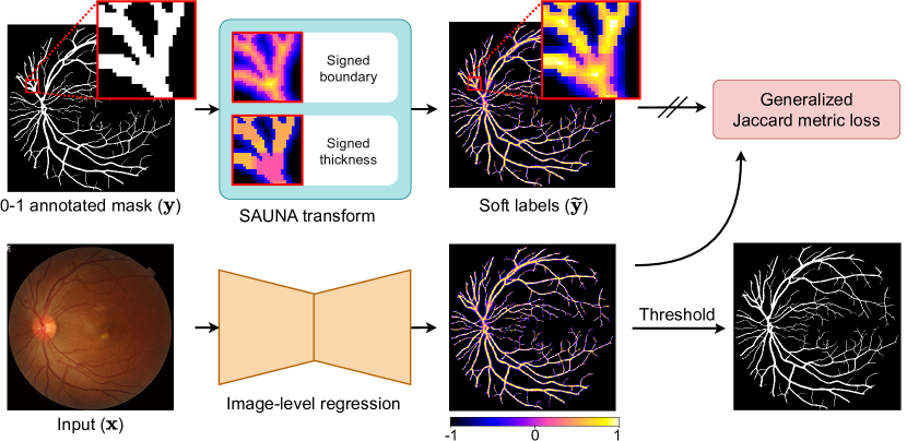
Figure 1: Our workflow of image-level regression for retinal image segmentation. Our primary contributions are the SAUNA transform (see Section 2.1) and an extension of the Jaccard metric loss [27] (see Section 2.2).

In semantic segmentation, the common training setup requires a collection of pairs of images and their corresponding segmentation masks (ground truth; GT), represented as $\mathbf{X}\times\mathbf{Y}$. To label a GT mask $\mathbf{y}\in\mathbf{Y}$, annotators categorize each pixel into foreground or background classes, thus termed a “hard label”. Using such GTs, DL models for semantic segmentation are usually trained as pixel-wise empirical risk minimization problems over a dataset [3]. Therefore, the majority of prior studies primarily rely on classification losses, such as cross-entropy loss and focal loss – for the task as follows: $\mathcal{L}_{\mathrm{PixelsCls}}=\frac{1}{D}\sum_{l=1}^{D}\ell_{\mathrm{CLS}}(f_{\theta}(\mathbf{x})_{i},\mathbf{y}_{i})$, where $D$ is the number of pixels, $f_{\theta}$ is a parametric segmentation model that takes an image $\mathbf{x}$ and predicts its respective segmentation mask. The term $\ell_{\mathrm{CLS}}(\cdot,\cdot)$ is typically the cross-entropy or focal loss. Moreover, another line of research focuses on optimizing the semantic segmentation task at the image level. As such, various segmentation losses – like Dice, Jaccard, Tversky, and Lovasz losses – have been developed to directly address the Dice score and Intersection-over-Union [18, 21, 2, 3]. Despite these advancements, those losses are originally designed for hard labels.

We argue that the aforementioned categorical pixel-wise labeling approach (0 or 1 in the case of vessel segmentation) implicitly overlooks the inherent annotation process uncertainty. In retinal images, vessels are typically not discernible due to factors such as blurry boundaries, thickness, and imaging quality. Many attempts have been made to consider this matter by softening human annotations, which discourages DL models from relying on the “fully certain” ground truth masks. Most prior studies tackle the problem using label smoothing techniques [19, 15, 1, 28, 27]. The idea of label smoothing is to provide the model information that one should not assign zero probability to BG pixels when labeling the FG ones, and it was first introduced in image classification [22]. Another line of work requires image-wise multi-annotations to model the uncertainty, which is highly expensive to obtain [19]. Other studies [14, 29] incorporate signed distance map regression as an auxiliary task alongside segmentation losses. Still, those studies commonly approach the medical segmentation problem as a pixel classification task.

In the retinal imaging domain, most of the prior studies also follow the trend of using hard labels. Similar to DL in general, most studies in this domain focus on improving DL architectures by advancing their capacity or embedding domain knowledge into architecture design [25, 16, 12, 24, 11, 13, 7, 26]. However, recent studies tend to look for an optimal trade-off between the model throughput and performance [12, 24, 11, 13, 7, 26]. Instead of standardizing input images into a reasonable size, those studies perform sliding windows over high-resolution retinal images, which is expensive for both training and evaluation. In our work, we characterize these techniques as patch-based methods and generally question such an approach.

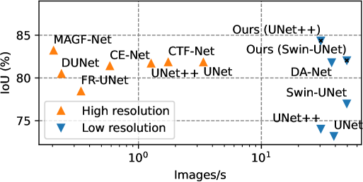
(a) Performance vs. throughput

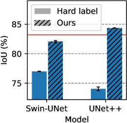
(b) Model improvements

Figure 2: Comparisons of performance and throughput across methods using high-resolution (HR) and low-resolution (LR) inputs on the FIVES test set. The x-axis of (a) is in log scale. The red line indicates the best result among the baselines. The corresponding quantitative results are in Table 1.

This work has several contributions (Figure 1). Firstly, we propose a new and simple method that tackles the segmentation problem as image-level regression. To achieve this, we propose a Segmentation Annotation UNcertainty-Aware (SAUNA) transform, inspired by the observation that it is hard to draw exact vessel boundaries, especially for thin vessels. The SAUNA transform generates a signed soft segmentation map $\tilde{\mathbf{y}}\in[-1,1]^{D}$ from $0-1$ annotated masks $\mathbf{y}$, without the need for multiple annotations per image. Specifically, positive and negative regions in $\tilde{\mathbf{y}}$ represent foreground (FG) and background (BG) respectively. As BG pixels distant from the FG’s vicinity are highly certain, the SAUNA transform explicitly marks them with the value $-1$. To train our model with these labels, we utilize the Jaccard metric loss (JML) [27]. We prove that this can be used beyond $[0,1]^{D}$ domain, which is the second contribution of this work. Finally, we conducted standardized and extensive experiments on $5$ retinal image datasets. Our findings indicate that while using high-resolution inputs can be beneficial, it is indeed possible to achieve both high performance and efficiency simultaneously (see Figure 2).

2 Proposed method

2.1 Segmentation Annotating UNcertainty-Aware (SAUNA) Transform

Let $\Omega=\{1,\dots,H\}\times\{1,\dots,W\}$ denote the set of pixel coordinates. For 0-1 annotated mask $\mathbf{y}$, we have $\mathbf{y}_{i}\in\{0,1\},\ \forall i\in\Omega$. We firstly define the unsigned shortest Euclidean distance and thickness transforms as follows

$$\mathbf{d}_{i} =\min_{j\in\Omega:\mathbf{y}_{j}\neq\mathbf{y}_{i}}\|i-j\|_{2},\quad i\in\Omega$$ (1)

$$\mathbf{t}_{i} =\max_{j\in C:\mathbf{y}_{i}=1,\left\|i-j\right\|_{\infty}\leq m}\mathbf{d}_{j},\quad i\in\Omega$$ (2)

where $C=\{j\in\Omega\mid\mathbf{d}_{j}\leq m\}$ is the set of pixels relatively close to FG regions, and $m=\max_{k\in\Omega,\mathbf{y}_{k}=1}\mathbf{d}_{k}$ represents the maximum Euclidean distance from FG pixels to their nearest boundary pixels. The thickness transform is defined as the application of max-pooling to a positive distance map. As the window size $m$ is significantly large by definition, locally maximal distance values are propagated across the region. Here, we respectively introduce the signed normalized boundary and thickness transforms as follows

$$\mathbf{y}^{B}_{i} =s(\mathbf{y}_{i})\cdot\min\left(1,\frac{\mathbf{d}_{i}}{m}\right),\quad i\in\Omega$$ (3)

$$\mathbf{y}^{T}_{i} =s(\mathbf{y}_{i})\cdot\left[1-\min\left(1,\frac{\mathbf{t}_{i}}{m}\right)\right],\quad i\in\Omega$$ (4)

where $s(\mathbf{y}_{i})=\operatorname{sign}(2\mathbf{y}_{i}-1)$. The minimum function is to ensure that we merely consider the neighboring regions of the boundaries, which implies ignoring distant BG pixels. $\mathbf{y}^{B}_{i}=0$ iff $i$ corresponds to a boundary pixel.

To this end, we propose the SAUNA transform based on boundary and thickness as the following

$$\tilde{\mathbf{y}}_{i}=\mathbf{y}^{B}_{i}+\mathbf{y}^{T}_{i}\in[-1,1],\quad i\in\Omega$$ (5)

In Figure 3, we provide a graphical illustration of how the SAUNA transform generates the signed soft labels from the 0-1 GT mask shown in Figure 3a. In Figure 3b, $\mathbf{y}^{B}$ generates a piece-wise function that exhibits irregular zig-zag behavior when the pixel is close enough to FG regions. For distant pixels that are highly certain, it becomes a constant function with a value of “-1”. $\mathbf{y}^{T}$ produces a step function whose value is inversely proportional to the thickness of either FG or BG region. The SAUNA map is derived from the summation of the two maps. This process preserves the behavior of $\mathbf{y}^{B}$ around the (easiest) thickest region while generating adaptive margins across the boundaries of (hard) thin ones. Intuitively, such a map encourages the image-level regression model to prioritize attention to challenging areas.

(a) GT

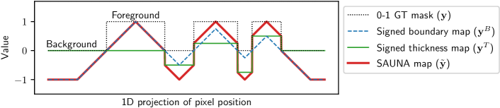
(b) Transition from the GT in (a) to a SAUNA map

Figure 3: Illustration of the transformation from a 0-1 ground truth (GT) mask to its associated SAUNA map (best viewed in color): (a) 2D GT mask with an orange projection, (b) corresponding transformations in the 1D projection.

2.2 Generalized Jaccard Metric Loss

JML introduced by Wang et al. [27] was originally designed for soft segmentation labels, and it was used for knowledge distillation [8]. The loss is formulated as

$$\Delta_{\mathrm{JML}}(\mathbf{a},\mathbf{b})=1-\frac{\left\|\mathbf{a}+\mathbf{b}\right\|_{1}-\left\|\mathbf{a}-\mathbf{b}\right\|_{1}}{\left\|\mathbf{a}+\mathbf{b}\right\|_{1}+\left\|\mathbf{a}-\mathbf{b}\right\|_{1}},$$ (6)

and is proven to be a metric for any $\mathbf{a},\mathbf{b}\in[0,1]^{D}$ [27]. The fact that the $\Delta_{\mathrm{JML}}$ loss is semi-metric or metric implies that $\forall\mathbf{a},\mathbf{b}\in[0,1]^{D},\Delta_{\mathrm{JML}}(\mathbf{a},\mathbf{b})=0\iff\mathbf{a}\equiv\mathbf{b}$, making it an objective that directly optimizes the IoU between the predictions and the soft labels. To perform the image-level regression task on the generated SAUNA maps in $[-1,1]^{D}$, we prove that the domain of $\Delta_{\mathrm{JML}}$ can be an arbitrary hypercube from $\mathbb{R}^{D}$, including $[-1,1]^{D}$.

Proposition 1 (Jaccard Metric Loss on a hypercube in $\mathbb{R}^{D}$)

$\Delta_{\mathrm{JML}}$ is a semi-metric in $[\alpha,\beta]^{D}\subseteq\mathbb{R}^{D}$. Specifically, $\forall\mathbf{a},\mathbf{b}\in[\alpha,\beta]^{D}$, we have

1. Reflexivity: $\Delta_{\mathrm{JML}}(\mathbf{a},\mathbf{b})=0\Longleftrightarrow\mathbf{a}\equiv\mathbf{b}$

2. Positivity: $\Delta_{\mathrm{JML}}(\mathbf{a},\mathbf{b})\geq 0$

3. Symmetry: $\Delta_{\mathrm{JML}}(\mathbf{a},\mathbf{b})=\Delta_{\mathrm{JML}}(\mathbf{b},\mathbf{a})$

Proof

See Suppl. Section 1.

Given any pair of an input image and its 0-1 annotated mask $(\mathbf{x},\mathbf{y})$, we utilize a parametric function $f_{\theta}$ to produce $\mathbf{f}=\tanh{f_{\theta}(\mathbf{x})}$, and apply the SAUNA transform on $\mathbf{y}$ to generate the soft label $\tilde{\mathbf{y}}$. Here, both $\mathbf{f}$ and $\tilde{\mathbf{y}}$ are in $[-1,1]^{D}$. To this end, we propose the generalized JML (GJML) as follows

$$\mathcal{L}_{\mathrm{GJML}}(\mathbf{f},\tilde{\mathbf{y}};\theta)=\Delta_{\mathrm{JML}}(\mathbf{f},\tilde{\mathbf{y}})=1-\frac{\left\|\mathbf{f}+\tilde{\mathbf{y}}\right\|_{1}-\left\|\mathbf{f}-\tilde{\mathbf{y}}\right\|_{1}}{\left\|\mathbf{f}+\tilde{\mathbf{y}}\right\|_{1}+\left\|\mathbf{f}-\tilde{\mathbf{y}}\right\|_{1}},\quad\forall\mathbf{f},\tilde{\mathbf{y}}\in[-1,1]^{D}$$ (7)

From Proposition 1, we have that $\mathcal{L}_{\mathrm{GJML}}$ is a semi-metric, which allows us to perform direct image-level regression for IoU maximization with soft labels.

3 Experiments

3.1 Experimental Setup

Datasets. Our experiments were conducted on 5 retinal datasets FIVES [10], DRIVE [20], STARE [9], CHASE-DB1, and HRF [4]. Among them, FIVES has significantly more samples than the other 4 datasets. The official data split of FIVES is $600$ for training and $200$ for testing. Meanwhile, DRIVE, STARE, CHASE-DB1, and HRF consist of $60$, $20$, $28$, and $45$ samples, respectively. These five datasets have different resolutions. As such, the image sizes of FIVES, DRIVE, STARE, CHASE-DB1, and HRF are $2048\times 2048$, $584\times 565$, $605\times 700$, $960\times 999$, and $2336\times 3504$, respectively.

Training and evaluation protocols. As FIVES is the largest dataset having at least $13$ times more samples than the other 4 datasets, we only utilized data from that dataset for training, and considered the others as external test sets. Specifically, we performed model selections on $600$ samples of the official FIVES training data split, while the remaining $200$ samples together with $153$ samples from the other datasets were kept for independent testing.

We investigated two input settings: low-resolution (LR) and high-resolution (HR). For LR, we resized the whole retinal image to $512\times 512$. For HR, we randomly cropped patches from HR retinal images, then we resized those patches to a common size of $512\times 512$. Thus, the two settings are called “full-image” and “patch-based” approaches, respectively. For our method, we adopted the efficient full-image setting.

Implementation details. We conducted our experiments on Nvidia V100 GPUs. Our method and baselines were implemented in Pytorch. To demonstrate our method on convolutional neural network and transformer-based network, we respectively employed UNet++ [30] and Swin-UNet [5] as the segmentation architecture. The soft-label baselines also used this network. We ensured that our method and baselines were trained using the same data preprocessing and augmentation pipeline. During training, we applied data augmentation using random flipping, rotation, color jittering, gamma correction, Gaussian noises, and cutout. Finally, we normalized the images with a mean of $[0.07,0.15,0.34]$ and a standard deviation of $[0.2,0.3,0.4]$, calculated from the training set of FIVES.

We used the Adam optimizer to train our method with an initial learning rate of $0.0001$ and a batch size of $4$. We employed $0$ as the threshold to binarize the SAUNA maps. While our method, as well as other full-image approaches, took $300$ epochs to train, we spent only $20$ epochs to train patch-based methods due to the enormous number of cropped patches (i.e. $800$ patches per retinal image).

We compared our method to a diverse set of SOTA references as listed in Table 1. Each method was re-trained $5$ times with different random seeds. For each random seed, we performed the $5$-fold cross-validation strategy for model selection. The prediction on each test input image was the average of the outputs from $5$ best models in each fold to reduce the effects of random data splitting on our results. For performance assessments, we adopted Dice score, intersection-over-union (IoU), sensitivity (Sens), specificity (Spec), and balanced accuracy (BA; an average of Sens and Spec). We reported image-wise means and standard errors (SE) of test metrics over $5$ runs.

Table 1: Performance comparisons between our method (highlighted in cyan) and a diverse set of baselines on the FIVES test set. The best results are highlighted in bold. “IN” indicates either HR or LR-based approach. All baseline methods were retrained on our data split for fair comparison.

Method	IN	GT	Loss	IoU	Dice	Sens	Spec	BA
IterNet [12]	High resolution	Hard labels	Dice + BCE	66.90±0.53	78.52±0.34	76.06±0.58	98.90±0.01	87.48±0.29
FR-UNet [13]				78.44±0.29	87.17±0.20	86.79±0.56	99.14±0.04	92.96±0.26
DUNet [24]				80.49±0.25	88.55±0.16	90.02±0.39	99.07±0.02	94.54±0.19
CE-Net [7]				81.40±0.13	89.14±0.08	90.75±0.24	99.13±0.01	94.94±0.12
UNet++ [30]				81.70±0.16	89.25±0.10	89.38±0.26	99.25±0.01	94.32±0.12
UNet [17]				81.84±0.16	89.39±0.10	90.94±0.26	99.12±0.01	95.03±0.12
CTF-Net [26]				81.85±0.16	89.51±0.10	90.33±0.26	99.22±0.01	94.78±0.12
MAGF-Net [11]				83.21±0.16	90.23±0.10	90.71±0.26	99.30±0.01	95.01±0.12
UNet [17]	Low resolution			73.21±0.18	84.15±0.12	84.08±0.23	98.86±0.01	91.47±0.11
UNet++ [30]				74.05±0.31	84.69±0.20	84.45±0.36	98.92±0.03	91.69±0.18
Swin-UNet [5]				77.00±0.04	86.52±0.03	88.12±0.10	98.93±0.01	93.53±0.04
D2SF [16]				80.68±0.20	89.30±0.12	86.52±0.24	99.44±0.03	92.98±0.12
DA-Net [25]				81.82±0.05	89.41±0.03	88.96±0.08	99.34±0.01	94.15±0.04
GeoLS [23, 27]			JML	79.66±0.25	88.12±0.14	91.08±0.39	98.91±0.07	94.99±0.16
LS [22, 27]			JML	80.47±0.27	88.57±0.17	88.14±1.04	99.27±0.09	93.70±0.48
BLS [27]			JML	81.77±0.07	89.43±0.04	90.09±0.29	99.23±0.03	94.66±0.13
Ours (Swin-UNet)			GJML	82.05±0.18	89.60±0.10	89.50±0.37	99.32±0.05	94.41±0.16
Ours (UNet++)		Soft labels	GJML	84.36±0.03	90.96±0.02	90.91±0.09	99.42±0.01	95.17±0.04

3.2 Results

FIVES dataset. We present the graphical illustrations in Figure 2a and the quantitative results in Table 1. In general, HR-based baselines performed substantially better than most of the LR-based counterparts. Out of all the baselines, MAGF-Net [11] attained the highest Dice and IoU scores. Despite our method being 149 times more computationally efficient compared to the top-performing baseline, it was the sole LR-based method to outperform the baseline across all metrics. Additionally, compared to DA-Net [25], the best LR-based method using hard labels, our method achieved substantial improvements of an IoU of $2.54\%$, a Dice of $1.55\%$, and a BA of $1.02\%$. Moreover, the combination of the SAUNA transform and GJML helped Swin-UNet and UNet++ gain significant improvements of $5.05\%$ and $10.31\%$ IoU, respectively (see Figure 2b). Furthermore, among the baselines using soft labels, the combination of BLS and JML [27] yielded the best performance. When compared to that baseline, our method performed $2.59\%$, $1.53\%$, and $0.55\%$ better in IoU, Dice, and BA, respectively. We visualize the quality results in Suppl. Figure S1.

Generalization to other datasets. After training the whole-image models on the FIVES dataset, we evaluated them on the 4 external datasets without finetuning. The quantitative results are illustrated in Table 2. Due to the changes in image scale, all methods suffered from a dip in IoU scores, but our method was the best at generalizing across all the external datasets. In comparison with the best baseline of Wang et al. [27], our method with UNet++ results in IoU gains of $1.3\%$, $0.3\%$, $0.5\%$, and $2.4\%$ on STARE, DRIVE, CHASEDB1, and HRF, respectively. Both the settings of our method substantially outperformed the corresponding baselines Swin-UNet and UNet++. Our setting with UNet++ demonstrated the most robust generalization.

Ablation study. We examined the impact of the signed distance transform and thickness information in Table 3. The vessel thickness on its own achieved poor segmentation quality, while the signed distance transform could deliver competitive performance. However, when the thickness was used to enrich the signed distance transform, the results were improved across $5$ metrics by at least $5$ standard errors.

Table 2: Generalization comparisons on the 4 external test sets (IoU means and SEs over 5 runs). Ours is marked in cyan. The best results are in bold.

Method	GT	STARE	DRIVE	CHASEDB1	HRF
UNet [17]	Hard labels	69.1±0.2	64.5±0.2	65.9±0.2	57.0±0.3
UNet++ [30]		69.8±0.2	64.7±0.4	66.5±0.1	56.9±0.5
DA-Net [25]		69.7±0.2	67.2±0.1	67.6±0.1	60.1±0.1
Swin-UNet [5]		68.5±0.1	65.0±0.1	64.3±0.1	59.2±0.1
GeoLS [23, 27]		69.9±0.1	68.1±0.1	65.8±0.2	57.5±0.2
LS [22, 27]		70.3±0.3	67.4±0.4	67.0±0.4	59.6±0.3
BLS [27]		71.0±0.1	68.1±0.1	67.2±0.1	61.0±0.2
Ours (Swin-UNet)		71.8±0.1	67.0±0.1	67.3±0.3	63.3±0.3
Ours (UNet++)	Soft labels	72.3±0.1	68.4±0.0	67.7±0.1	63.4±0.1

Table 3: Ablation study on the SAUNA transform.

Setting	IoU	Dice	Sens	Spec	BA
SAUNA	84.36±0.03	90.96±0.02	90.91±0.09	99.42±0.01	95.17±0.04
without $\mathbf{y}^{T}$	82.80±0.03	90.09±0.02	90.06±0.12	99.33±0.01	94.70±0.05
without $\mathbf{y}^{B}$	67.16±2.07	79.65±1.50	88.32±0.27	97.62±0.32	92.97±0.18

4 Conclusions

In this work, we have presented a regression-based approach to retinal vessel segmentation. We utilized the newly developed SAUNA transform to generate soft labels, motivated by the uncertainty in the annotation process. We leveraged the Jaccard metric loss [27] and proved that it is a semi-metric loss on arbitrary hypercubes. Through rigorous experimental evaluation, we showed that our method outperforms existing methods on an in-domain test set (i.e. FIVES), and generalizes better compared to low-resolution references on external datasets. Our empirical results question the need for using high-resolution images for retinal image segmentation. Our code and computational benchmark will be made publicly available.

1 Proof of Proposition 1

Proof

For any $\mathbf{a},\mathbf{b}\in[\alpha,\beta]^{D}$, JML is defined in [27] as

$$\Delta_{\mathrm{JML}}(\mathbf{a},\mathbf{b})=1-\frac{\left\|\mathbf{a}+\mathbf{b}\right\|_{1}-\left\|\mathbf{a}-\mathbf{b}\right\|_{1}}{\left\|\mathbf{a}+\mathbf{b}\right\|_{1}+\left\|\mathbf{a}-\mathbf{b}\right\|_{1}}.$$ (8)

(i) Reflexivity.

If $\Delta_{\mathrm{JML}}(\mathbf{a},\mathbf{b})=0$, we can derive $\|\mathbf{a}-\mathbf{b}\|_{1}=\sum_{i=1}^{D}|\mathbf{a}_{i}-\mathbf{b}_{i}|=0$. Thus, we have $\mathbf{a}_{i}=\mathbf{b}_{i},\forall i=1..D$, which is equivalent to $\mathbf{a}\equiv\mathbf{b}$.

If $\mathbf{a}\equiv\mathbf{b}$, we obviously have $\Delta_{\mathrm{JML}}(\mathbf{a},\mathbf{b})=0$.

(ii) Positivity.

The property is satisfied because we can rewrite $\Delta_{\mathrm{JML}}$ as follows

$$\Delta_{\mathrm{JML}}(\mathbf{a},\mathbf{b})=\frac{2\left\|\mathbf{a}-\mathbf{b}\right\|_{1}}{\left\|\mathbf{a}+\mathbf{b}\right\|_{1}+\left\|\mathbf{a}-\mathbf{b}\right\|_{1}}\geq 0,\quad\forall\mathbf{a},\mathbf{b}\in[\alpha,\beta]^{D}$$ (9)

(iii) Symmetry.

As $\|\mathbf{a}+\mathbf{b}\|_{1}=\|\mathbf{b}+\mathbf{a}\|_{1}$ and $\|\mathbf{a}-\mathbf{b}\|_{1}=\|\mathbf{b}-\mathbf{a}\|_{1},\forall\mathbf{a},\mathbf{b}\in[\alpha,\beta]^{D}$, we obviously have $\Delta_{\mathrm{JML}}(\mathbf{a},\mathbf{b})=\Delta_{\mathrm{JML}}(\mathbf{b},\mathbf{a})$ and this concludes the proof.

Figure S1: Visualization of predictions of our method and the baselines on the test sets. HR indicates the method using high-resolution input images. The overlaid values are IoU scores. Green, black, blue, and red pixels indicate true positive, true negative, false positive, and false negative, respectively.

References

- [1] Alcover-Couso, R., Escudero-Vinolo, M., SanMiguel, J.C.: Soft labelling for semantic segmentation: Bringing coherence to label down-sampling. arXiv preprint arXiv:2302.13961 (2023)
- [2] Berman, M., Triki, A.R., Blaschko, M.B.: The lovász-softmax loss: A tractable surrogate for the optimization of the intersection-over-union measure in neural networks. In: Proceedings of the IEEE conference on computer vision and pattern recognition. pp. 4413–4421 (2018)
- [3] Bertels, J., Eelbode, T., Berman, M., Vandermeulen, D., Maes, F., Bisschops, R., Blaschko, M.B.: Optimizing the dice score and jaccard index for medical image segmentation: Theory and practice. In: Medical Image Computing and Computer Assisted Intervention–MICCAI 2019: 22nd International Conference, Shenzhen, China, October 13–17, 2019, Proceedings, Part II 22. pp. 92–100. Springer (2019)
- [4] Budai, A., Bock, R., Maier, A., Hornegger, J., Michelson, G., et al.: Robust vessel segmentation in fundus images. International journal of biomedical imaging 2013 (2013)
- [5] Cao, H., Wang, Y., Chen, J., Jiang, D., Zhang, X., Tian, Q., Wang, M.: Swin-unet: Unet-like pure transformer for medical image segmentation. In: European conference on computer vision. pp. 205–218. Springer (2022)
- [6] Fraz, M.M., Remagnino, P., Hoppe, A., Uyyanonvara, B., Rudnicka, A.R., Owen, C.G., Barman, S.A.: An ensemble classification-based approach applied to retinal blood vessel segmentation. IEEE Transactions on Biomedical Engineering 59(9), 2538–2548 (2012)
- [7] Gu, Z., Cheng, J., Fu, H., Zhou, K., Hao, H., Zhao, Y., Zhang, T., Gao, S., Liu, J.: Ce-net: Context encoder network for 2d medical image segmentation. IEEE transactions on medical imaging 38(10), 2281–2292 (2019)
- [8] Hinton, G., Vinyals, O., Dean, J.: Distilling the knowledge in a neural network. arXiv preprint arXiv:1503.02531 (2015)
- [9] Hoover, A., Kouznetsova, V., Goldbaum, M.: Locating blood vessels in retinal images by piecewise threshold probing of a matched filter response. IEEE Transactions on Medical imaging 19(3), 203–210 (2000)
- [10] Jin, K., Huang, X., Zhou, J., Li, Y., Yan, Y., Sun, Y., Zhang, Q., Wang, Y., Ye, J.: Fives: A fundus image dataset for artificial intelligence based vessel segmentation. Scientific Data 9(1), 475 (2022)
- [11] Li, J., Gao, G., Liu, Y., Yang, L.: Magf-net: A multiscale attention-guided fusion network for retinal vessel segmentation. Measurement 206, 112316 (2023)
- [12] Li, L., Verma, M., Nakashima, Y., Nagahara, H., Kawasaki, R.: Iternet: Retinal image segmentation utilizing structural redundancy in vessel networks. In: Proceedings of the IEEE/CVF winter conference on applications of computer vision. pp. 3656–3665 (2020)
- [13] Liu, W., Yang, H., Tian, T., Cao, Z., Pan, X., Xu, W., Jin, Y., Gao, F.: Full-resolution network and dual-threshold iteration for retinal vessel and coronary angiograph segmentation. IEEE Journal of Biomedical and Health Informatics 26(9), 4623–4634 (2022)
- [14] Liu, Z., He, X., Lu, Y.: Combining unet 3+ and transformer for left ventricle segmentation via signed distance and focal loss. Applied Sciences 12(18), 9208 (2022)
- [15] Ma, J., Wang, C., Liu, Y., Lin, L., Li, G.: Enhanced soft label for semi-supervised semantic segmentation. In: Proceedings of the IEEE/CVF International Conference on Computer Vision. pp. 1185–1195 (2023)
- [16] Qiu, Z., Hu, Y., Chen, X., Zeng, D., Hu, Q., Liu, J.: Rethinking dual-stream super-resolution semantic learning in medical image segmentation. IEEE Transactions on Pattern Analysis and Machine Intelligence (2023)
- [17] Ronneberger, O., Fischer, P., Brox, T.: U-net: Convolutional networks for biomedical image segmentation. In: Medical Image Computing and Computer-Assisted Intervention–MICCAI 2015: 18th International Conference, Munich, Germany, October 5-9, 2015, Proceedings, Part III 18. pp. 234–241. Springer (2015)
- [18] Salehi, S.S.M., Erdogmus, D., Gholipour, A.: Tversky loss function for image segmentation using 3d fully convolutional deep networks. In: International workshop on machine learning in medical imaging. pp. 379–387. Springer (2017)
- [19] Silva, J.L., Oliveira, A.L.: Using soft labels to model uncertainty in medical image segmentation. arXiv preprint arXiv:2109.12622 (2021)
- [20] Staal, J., Abràmoff, M.D., Niemeijer, M., Viergever, M.A., Van Ginneken, B.: Ridge-based vessel segmentation in color images of the retina. IEEE transactions on medical imaging 23(4), 501–509 (2004)
- [21] Sudre, C.H., Li, W., Vercauteren, T., Ourselin, S., Jorge Cardoso, M.: Generalised dice overlap as a deep learning loss function for highly unbalanced segmentations. In: Deep Learning in Medical Image Analysis and Multimodal Learning for Clinical Decision Support: Third International Workshop, DLMIA 2017, and 7th International Workshop, ML-CDS 2017, Held in Conjunction with MICCAI 2017, Québec City, QC, Canada, September 14, Proceedings 3. pp. 240–248. Springer (2017)
- [22] Szegedy, C., Vanhoucke, V., Ioffe, S., Shlens, J., Wojna, Z.: Rethinking the inception architecture for computer vision. In: Proceedings of the IEEE conference on computer vision and pattern recognition. pp. 2818–2826 (2016)
- [23] Vasudeva, S.A., Dolz, J., Lombaert, H.: Geols: Geodesic label smoothing for image segmentation. In: Medical Imaging with Deep Learning (2023)
- [24] Wang, B., Qiu, S., He, H.: Dual encoding u-net for retinal vessel segmentation. In: Medical Image Computing and Computer Assisted Intervention–MICCAI 2019: 22nd International Conference, Shenzhen, China, October 13–17, 2019, Proceedings, Part I 22. pp. 84–92. Springer (2019)
- [25] Wang, C., Xu, R., Xu, S., Meng, W., Zhang, X.: Da-net: Dual branch transformer and adaptive strip upsampling for retinal vessels segmentation. In: International Conference on Medical Image Computing and Computer-Assisted Intervention. pp. 528–538. Springer (2022)
- [26] Wang, K., Zhang, X., Huang, S., Wang, Q., Chen, F.: Ctf-net: Retinal vessel segmentation via deep coarse-to-fine supervision network. In: 2020 IEEE 17th International Symposium on Biomedical Imaging (ISBI). pp. 1237–1241. IEEE (2020)
- [27] Wang, Z., Blaschko, M.B.: Jaccard metric losses: Optimizing the jaccard index with soft labels. arXiv preprint arXiv:2302.05666 (2023)
- [28] Wang, Z., Popordanoska, T., Bertels, J., Lemmens, R., Blaschko, M.B.: Dice semimetric losses: Optimizing the dice score with soft labels. arXiv preprint arXiv:2303.16296 (2023)
- [29] Xue, Y., Tang, H., Qiao, Z., Gong, G., Yin, Y., Qian, Z., Huang, C., Fan, W., Huang, X.: Shape-aware organ segmentation by predicting signed distance maps. In: Proceedings of the AAAI Conference on Artificial Intelligence. vol. 34, pp. 12565–12572 (2020)
- [30] Zhou, Z., Siddiquee, M.M.R., Tajbakhsh, N., Liang, J.: Unet++: Redesigning skip connections to exploit multiscale features in image segmentation. IEEE transactions on medical imaging 39(6), 1856–1867 (2019)