SiNGR: Brain Tumor Segmentation via Signed Normalized Geodesic Transform Regression

Abstract

One of the primary challenges in brain tumor segmentation arises from the uncertainty of voxels close to tumor boundaries. However, the conventional process of generating ground truth segmentation masks fails to treat such uncertainties properly. Those “hard labels” with 0s and 1s conceptually influenced the majority of prior studies on brain image segmentation. As a result, tumor segmentation is often solved through voxel classification. In this work, we instead view this problem as a voxel-level regression, where the ground truth represents a certainty mapping from any pixel based on the distance to tumor border. We propose a novel ground truth label transformation, which is based on a signed geodesic transform, to capture the uncertainty in brain tumors’ vicinity, while maintaining a margin between positive and negative samples. We combine this idea with a Focal-like regression L1-loss that enables effective regression learning in high-dimensional output space by appropriately weighting voxels according to their difficulty. We thoroughly conduct an experimental evaluation to validate the components of our proposed method, compare it to a diverse array of state-of-the-art segmentation models, and show that it is architecture-agnostic. The code of our method is made publicly available at https://github.com/Oulu-IMEDS/SiNGR/.

1 Introduction

Glioma is the most prevalent type of brain tumor in adults, which is also the leading cause of cancer deaths for men under 40 years old and women under 20 years old [17]. Timely detection and characterization of gliomas is crucial for patient survival. Fortunately, the widespread availability of magnetic resonance imaging (MRI) enables non-invasive quantitative brain assessments, enabling healthcare professionals to detect and closely monitor the progression of brain tumors [21]. In response to this, various studies have been conducted to develop deep learning (DL)-based methods for segmentation of brain tumors’ volumes from MR images [20, 8, 7, 25]. In this paper, so as it is done conventionally, by segmentation we imply semantic segmentation (SSEG), the goal of which is to categorize each element (voxel or pixel) within an image into background and foreground classes.

In the existing literature on brain tumor segmentation, the first line of research aims to improve the effectiveness of DL architectures by increasing the model capacity and/or embedding domain knowledge into architecture design [7, 16, 26, 23, 8]. The second line of research studies novel segmentation losses that are preferably correlated with metrics of interest such as Dice score or Intersection-of-Union (IoU) [3, 2, 15, 25, 24]. Finally, the third group of studies investigates alternative ways to define the ground truth (GT) masks through soft labels [20, 12]. Our study is at the intersection of the last two directions, as we aim to define the GT masks through soft labels, as well as to develop a new loss function for the problem.

SSEG is typically modeled as voxel-wise classification [7, 16, 26, 23, 8]. This might be inherited from the annotation process of GT masks, where each voxel is assigned to one or more classes by human annotators. However, such strictly defined categories (e.g. $0$ vs $1$ in the binary case) in the segmentation masks imply an equal role for all voxels when it comes to determining the edges of an object of interest in an image. Such an approach fails to capture the intra-class uncertainty in the annotation masks. Delineating complex non-rigid structures such as tumors in low-resolution MR images is highly challenging, and the uncertainty one can easily identify could come from technical image quality, visibility, detail complexity, and the knowledge of the annotator.

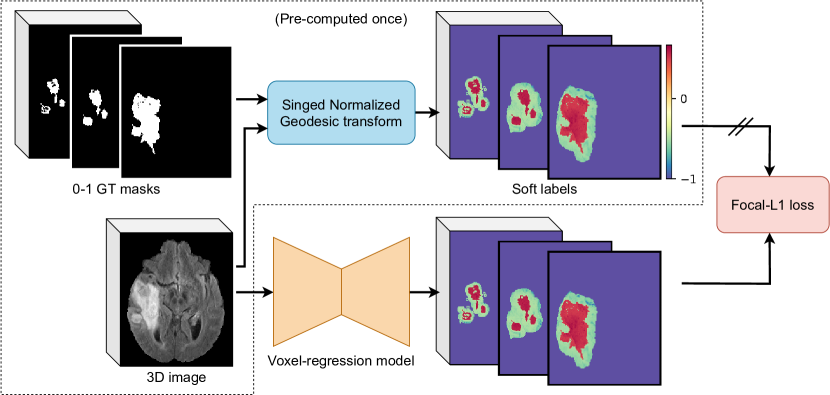
Figure 1: The overview of Signed Normalized Geodesic transform Regression (SiNGR).

Some studies [20, 12, 25, 24] attempted to develop soft labels for SSEG, which allows the model to learn that it should not always be a certainty. One such example is label smoothing. This technique relies on the number of classes [18], which is not suitable for the aforementioned intra-class uncertainty. Liu et al. [11] proposed to produce soft labels using the signed Euclidean distance map (SDM). Nevertheless, the SDM regression was merely considered as a regularizer for the segmentation task. Vasudeva et al. [20] employed the unsigned geodesic distance (GeoDT) transform [19] to generate a novel type of soft labels that can characterize both spatial distance and image gradient. Yet unsigned GeoDT-based soft labels were then integrated into the cross-entropy (CE) loss, which is a classification loss.

We observe that the complexity of the segmentation annotation process is in the labeling of voxels around the boundaries of objects of interest (OOI). The uncertainty of a voxel’s label is proportional to the inverse of its distance to the nearest boundary, as well as the visual blurriness in this region. Although unsigned GeoDT naturally allows us to capture these properties, additional signals are needed to differentiate foreground from background voxels. Moreover, voxels significantly distant from the OOI exhibit very low uncertainty; thus, these voxels should be marked in a manner that directs the model to pay less attention to them.

In this study, we formulate the SSEG problem as voxel regression (see Figure 1). We propose an extension of the unsigned GeoDT [19], termed Signed Normalized Geodesic (SiNG) transform that aims to approximate modeling of segmentation annotations done by human from input images and the corresponding GT masks. The SiNG transform is designed to primarily focus on the vicinity of the OOI by assigning values in $(0,1]$ to foreground (FG) regions, values in $(-1,0]$ to nearby background (BG) regions, and $-1$’s to distant voxels. As we perform SSEG via SiNG transform Regression, our method is named SiNGR. To handle the imbalance of FG and BG voxels, we introduce a novel regression loss, termed Focal-L1 loss. We conduct standardized and thorough experiments to demonstrate the effectiveness of our method on the BraTS and LGG FLAIR datasets. The empirical evidence shows that our method is beneficial for various DL architectures.

2 Method

2.1 Overview

We approach the SSEG problem via signed soft-label regression. Specifically, we utilize the SiNG transform presented in Section 2.2 to convert 0-1 GT masks to signed soft labels, where regions of interest and BG regions are represented by positive and negative values respectively. The proposed transform is designed in such a way that FG and BG voxels are marginally separate across $0$, which allows a simple $0$-threshold post-processing step to produce final predicted masks. To effectively train the regression task, we introduce a novel loss, named Focal-L1, in Section 2.3.

2.2 Signed Normalized Geodesic Transform

2.2.1 Unsigned transform.

Given an input image $I$ with spatial dimensions of $H\times W\times L$, and an arbitrary-shaped region $R\subset\Omega=[H]\times[W]\times[L]$ with $[N]=\{1,\dots,N\}$, an L1-based unsigned geodesic distance transform (GeoDT) from a point $i\in\Omega$ to $R$ is defined as [19, 22]

$$G^{\lambda}(i;R,I) =\min_{j\in R}D^{\lambda}(i,j,I),$$ (1)

$$D^{\lambda}(i,j;I) =\min_{p\in P_{i,j}}\int_{0}^{1}(1-\lambda)\|p^{\prime}(s)\|_{1}+\lambda\|\nabla I(p(s))\cdot u(s)\|_{1}$$ (2)

where $\lambda\in[0,1]$ is a weighting hyperparameter, $P(i,j)$ is the set of all paths between locations $i$ and $j$, $p$ is a feasible parameterized path, $u(s)=\frac{p^{\prime}(s)}{\|p^{\prime}(s)\|_{1}}$, and $\nabla I(p(s))$ represents image gradient at $p(s)$. Here, we have that $G^{\lambda}(i,R,I)=0\ \forall i\in R,\ \forall\lambda\in[0,1]$. Intuitively, the unsigned GeoDT calculates the cost of the shortest path from point $i$ to the region $R$ based on both distance and image gradient information. The integral makes GeoDT computationally expensive when we apply the transform for the whole image. Its cost is proportional to $R$’s cardinality for Eq. 1 and $I$’s size due to Eq. 2.

2.2.2 Signed version.

For signed GeoDT, one typically runs the GeoDT transform twice for the foreground and background regions, which is intensively costly [6]. To speed up the signed GeoDT, we merely consider a set $R_{B}$ of boundary voxels of OOI extracted from a 0-1 segmentation mask $M$ using the Canny edge detector [5]. Hereinafter, as $R_{B}$ is our primary region of interest, we omit $R_{B}$ and $I$ from Eq. 1 for simplicity, that is $G^{\lambda}_{i}=G^{\lambda}(i;R_{B},I)$. Given $R_{B}$, we apply unsigned GeoDT for the whole image to produce an unsigned map. Afterwards, we rely on $M$ to specify the signs of the obtained map, that is $s_{i}G^{\lambda}_{i},\forall i\in\Omega$, where $s_{i}=\mathrm{sign}(2M_{i}-1)$ is the sign of voxel $i$. As the uncertainty of human annotations is primarily around the boundary $R_{B}$, we thus ignore regions substantially far from the boundary. As such, we let $\lambda=0$, and define the neighboring region of the boundary

$$\mathcal{B} =\left\{i\in\Omega\mid G^{0}_{i}\leq\beta\right\}$$ (3)

$$\mathrm{s.t.}\ \beta =\max_{i\in\Omega:M_{i}=1}G^{0}_{i}$$ (4)

where $\beta$ represents the maximum spatial distance (i.e. the latter term in Eq. 2 is omitted when $\lambda=0$). Finally, we propose the SiNG transform as follows

$$\mathcal{S}_{i}=\left\{\begin{matrix}\frac{1}{\tau}(1-\delta)s_{i}G^{\lambda}_{i}+\delta s_{i}&\quad\ \mathrm{if}\ i\in\mathcal{B}\\ -1&\quad\ \mathrm{otherwise}\end{matrix}\right.$$ (5)

where $\tau=\max_{j\in\mathcal{B}}G^{\lambda}_{j}$ is a normalization constant for each pair $(I,M)$, and $\delta\in[0,1)$ is a margin hyperparameter. The margin $\delta$ is needed to ensure the discrepancy in the signed normalized map between foreground and background voxels.

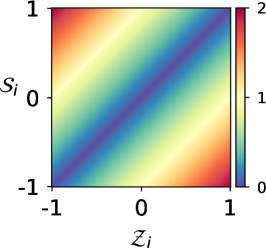
(a) L1 loss

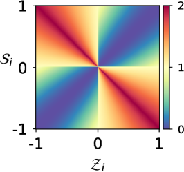
(b) Focal-L1 loss ($\gamma=1$)

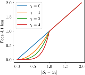
(c) Focal-L1 behavior

Figure 2: Comparison between L1 and Focal-L1 losses: (a-b) 2D loss surfaces, and (c) a behavior of the proposed Focal-L1 loss. Colors in (a-b) represent loss magnitudes. In (c), we assume that $|\mathcal{S}_{i}|=1$ or $|\mathcal{Z}_{i}|=1,\forall i\in\Omega$.

2.3 Focal-L1 Loss

We formulate the tumor segmentation task as image-level “regression” rather than voxel “classification”, where one commonly utilizes the cross-entropy (CE) or focal loss for the optimization. In alignment with the preceding subsection, we also consider the significance of diversity across various regions. As such, the regression loss is supposed to prioritize hard regions over easy ones. Inspired by the CE-based focal loss [10], we propose the following L1-based focal loss, namely Focal-L1, for the regression task.

Given an arbitrary pair of inputs $(I,M)$, we utilize the SiNG transformation to produce a corresponding map $\mathcal{S}$ with a certain $\lambda$. In addition, assuming that we have a parametric function $f_{\theta}$ with parameters $\theta$, and $f_{\theta}(I)$ denotes a predicted mask from the input image $I$. We then utilize the tanh function to convert values of $f_{\theta}(I)$ into the range $[-1,1]$, that is $\mathcal{Z}=\tanh(f_{\theta}(I))$. To this end, we propose the Focal-L1 loss as follows

$$\mathcal{L}_{\mathrm{FocalL1}}(\mathcal{S},\mathcal{Z};\theta)=\frac{1}{|\Omega|}\sum_{i\in\Omega}|\mathcal{S}_{i}-\mathcal{Z}_{i}|\underbrace{\frac{|\mathcal{S}_{i}-\mathcal{Z}_{i}|^{\gamma\mathbbm{I}(\mathcal{S}_{i}\mathcal{Z}_{i}\geq 0)}}{\max(|\mathcal{S}_{i}|,|\mathcal{Z}_{i}|)+\varepsilon}}_{\mathrm{Sample\ weighting}},$$ (6)

where $\varepsilon$ is a positive constant to avoid numerical issues, $\gamma$ is a positive hyperparameter, and $\mathbb{I}(\cdot)$ is the indicator function. A graphical comparison between our loss and the L1 loss is presented in Figure 2. Note that the backpropagation is not applied to the weighting term. Whereas the weighting term’s numerator is fixed at $1$ for hard cases ($\mathcal{S}_{i}\mathcal{Z}_{i}<0$), it is scaled down to less than $1$ for easy ones ($\mathcal{S}_{i}\mathcal{Z}_{i}\geq 0$). Meanwhile, the denominator reduces the importance of highly certain voxels (with high absolute value), as they are straightforward to predict. Overall, the sample weighting helps the loss to prioritize enforcing difficult voxels over simple ones.

3 Experiments

Table 1: Performance comparisons between our methods and the SOTA baselines on the BraTS test set (means and SEs over $5$ random seeds). The best results with substantial differences are highlighted in bold.

Method	GT	Dice score (%) $\uparrow$				HD95 ($mm$) $\downarrow$
		ET	TC	WT	Avg	ET	TC	WT	Avg
TransBTS [23]	Hard label	81.0±0.3	83.0±0.4	90.4±0.1	84.8±0.2	4.2±0.3	6.4±0.2	6.4±0.1	5.7±0.2
SegResnet [14]		81.1±0.3	85.5±0.3	90.7±0.1	85.8±0.2	3.3±0.1	5.5±0.3	5.7±0.4	4.9±0.2
UNETR [8]		82.3±0.2	82.0±0.4	90.0±0.1	84.8±0.2	4.0±0.3	7.4±0.2	6.2±0.4	5.9±0.2
EoFormer [16]		82.5±0.2	84.8±0.4	91.3±0.0	86.2±0.2	3.7±0.2	6.4±0.4	5.9±0.3	5.3±0.2
UNet++3D [28]		83.1±0.1	86.0±0.2	90.9±0.2	86.7±0.1	4.4±0.4	6.3±0.3	5.7±0.3	5.5±0.3
UNet3D [9]		83.1±0.2	86.1±0.3	90.4±0.2	86.5±0.1	3.8±0.4	5.9±0.3	6.5±0.6	5.4±0.4
NestedFormer [26]		83.5±0.1	85.4±0.1	91.2±0.1	86.7±0.1	4.4±0.4	7.4±0.4	6.6±0.4	6.1±0.4
Swin-UNETR [7]		84.1±0.2	85.7±0.4	90.9±0.1	86.9±0.2	3.7±0.3	6.4±0.2	6.0±0.2	5.4±0.2
Ours (Swin-UNETR)	SiNG	85.1±0.3	88.0±0.1	91.3±0.1	88.1±0.1	2.3±0.1	4.2±0.2	4.8±0.0	3.8±0.1

3.1 Setup

Datasets. We thoroughly conducted experiments on two public brain tumor datasets: BraTS 2020 and LGG FLAIR. BraTS 2020 [13] consists of multi-modal MR images from $369$ subjects. Each image was aligned across four modalities and was standardized to a volume size of $240\times 240\times 155$. The segmentation targets are enhancing tumor (ET), tumor core (TC), and whole tumor (WT). We divided the dataset into three portions with $236$, $59$, and $74$ samples for training, validation, and test sets, respectively. LGG FLAIR [4] has $110$ 3-channel FLAIR MR images and corresponding abnormality segmentation masks. The number of axial slices of each MR scan varies from $20$ to $80$, and they have a common spatial dimension of $256\times 256$. We split the data into training, validation, and test sets with $70$, $18$, and $22$ samples, respectively.

Implementation details. All models were trained on Nvidia V100 GPUs. We implemented our pipeline using Pytorch and followed a standard data processing configuration for all methods. We used the FastGeodist library to compute unsigned GeoDT maps [1]. During the training process on BraTS, the 3D MR images were randomly cropped to $128\times 128\times 128$ cubes, and augmented by flipping, intensity scaling, and intensity shifting. We performed the window-slicing technique with a window size of $128\times 128\times 128$ in the validation and test stages. We utilized the Adam optimizer with an initial learning rate of $10^{-4}$, a weight decay of $10^{-5}$, and a batch size of $2$. Regarding SiNGR-specific hyperparameters, we empirically found $\lambda=0.5$ and $\gamma=1$ working the best. The hyperparameter $\varepsilon$ in Eq. 6 was set to $0.0$. We performed $0$-thresholding to binarize our predicted maps. For performance evaluation, we utilized image-wise IoU, Dice score, and $95\%$ Hausdorff distance (HD95).

We compared our method to a diverse array of references specializing in 3D data as listed in Tables 1 and 2. In addition, we validated the SiNG transform and the Focal-L1 loss against other soft-label baselines – namely label smoothing (LS) [18] and Geodesic label smoothing (GeoLS) [20] – together with Jaccard metric loss (JML) [24], which specializes in optimizing with soft labels.

Table 2: Performance comparisons between our methods and the SOTA baselines on the LGG FLAIR test set (means and SEs over $5$ random seeds). The best results are highlighted in bold.

Method	GT	IoU (%) $\uparrow$	Dice (%) $\uparrow$	HD95 ($mm$) $\downarrow$
EoFormer [16]	Hard label	38.8±11.3	68.4±3.0	27.1±5.1
NestedFormer [26]		46.6±3.1	60.4±1.1	58.4±1.7
UNETR [8]		49.5±3.2	62.8±1.0	49.5±1.8
SegResnet [14]		50.5±1.5	64.9±0.5	46.3±2.1
UNet++3D [28]		59.0±3.3	71.1±1.1	34.6±1.3
Swin-UNETR [7]		54.4±2.3	67.8±0.8	32.2±1.8
TransBTS [23]		58.5±1.1	71.9±0.5	24.8±2.4
UNet3D [9]		57.9±4.0	69.1±1.3	33.6±2.0
Ours (UNet3D)	SiNG	71.4±0.7	82.3±0.5	11.4±1.6

(a) Dice on BraTS

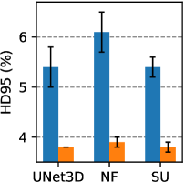
(b) HD95 on BraTS

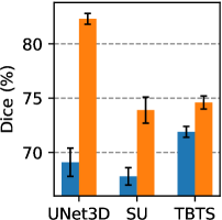
(c) Dice on LGG

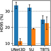
(d) HD95 on LGG

Figure 3: Pair-wise comparisons between baselines using hard labels (in blue) and our method (in orange) across different architectures and metrics. NF, SU, and TBTS mean NestedFormer, Swin-UNETR, and TransBTS respectively.

3.2 Results

BraTS 2020 dataset. The quantitative results on the BraTS test set are presented in Table 1. Accordingly, the top-3 methods with the highest IoU used the UNet3D, NestedFormer, and Swin-UNETR architectures. When we applied our SiNGR method to those three architectures, we observed consistent and substantial improvements in all the metrics (see Figures 3a and 3b). For instance, compared to the best baseline, Swin-UNETR, our corresponding method achieved $1.2\%$ and $1.6mm$ better in average Dice score and average HD95, respectively. We present a qualitative comparison of the methods in Suppl. Figure S1.

LGG FLAIR dataset. We present the detailed results on the LGG FLAIR test set in Table 2. On this small dataset, the impact of SiNGR was particularly significant on UNet3D, and this setting also acquired the highest IoU and Dice score. Compared to the UNet3D reference, our method resulted in significant gains of $13.5\%$ IoU, $13.2\%$ Dice score, and $22.2mm$ HD95. Using our method also consistently led to substantial improvements for Swin-UNETR and TransBTS (see Figures 3c and 3d). The qualitative results are presented in Suppl. Figure S2.

Impact of SiNG and Focal-L1. We investigated the effects of the components of our method and demonstrated the results on the BraTS test set in Table 3. Two unsigned label smoothing techniques [18, 20] did not perform well on the task. Compared to LS, our method outperformed with differences of $8.4\%$ and $7.8mm$ in average Dice score and average HD95, respectively. Additionally, among L1, L2, and product [27] losses, L1 was the best combination with the SiNG transform. However, L1 setting achieved an average Dice of $1.1\%$ lower than our method. Moreover, the empirical evidence showed the importance of the margin in the SiNG transform as well as the sample weighting coefficient in Focal-L1 loss. Notably, excluding the margin $\delta$ in SiNG led to a substantial drop of $3.4\%$ average Dice score and an increase of $1.5mm$ average HD95.

Table 3: Performance comparisons between different combinations of soft labels and loss functions on BraTS. UNet3D was the common architecture. $\delta$ is the margin in SiNG. Focal-L1^† indicates that the sample weighting in Eq. 6 is simplified to $|\mathcal{S}_{i}-\mathcal{Z}_{i}|^{\gamma}$. Our optimal setting is highlighted in cyan.

Label	$\delta$	Loss	Dice score (%) $\uparrow$				HD95 ($mm$) $\downarrow$
			ET	TC	WT	Avg	ET	TC	WT	Avg
LS [18]	-	JML [24]	75.5±1.2	75.5±0.7	87.5±0.3	79.5±0.6	5.7±0.4	17.8±4.5	11.2±1.5	11.6±2.1
GeoLS [20]	-	JML [24]	67.0±0.9	63.3±2.3	80.8±0.7	70.4±1.1	20.5±1.7	12.2±0.9	24.3±2.7	19.0±1.5
SiNG	0.5	L2	80.9±0.1	84.3±0.2	90.4±0.1	85.2±0.1	3.9±0.4	5.9±0.3	6.3±0.4	5.4±0.3
		Product [27]	82.5±0.4	86.9±0.1	90.9±0.1	86.8±0.2	3.9±0.5	5.6±0.4	5.5±0.3	5.0±0.4
		L1	82.7±0.1	87.1±0.3	90.7±0.1	86.8±0.1	3.3±0.3	4.9±0.2	5.6±0.2	4.6±0.2
		Focal-L1†	83.4±0.3	87.1±0.2	91.0±0.1	87.1±0.2	3.1±0.4	4.8±0.4	5.2±0.2	4.3±0.3
	0		80.0±0.5	83.8±0.5	89.9±0.1	84.5±0.3	4.3±0.3	5.8±0.4	5.7±0.1	5.3±0.3
	0.5	Focal-L1	84.4±0.1	88.1±0.1	91.1±0.1	87.9±0.0	2.5±0.1	4.2±0.1	4.8±0.0	3.8±0.0

4 Conclusions

We have introduced a simple approach to segmentation of brain tumors through voxel-wise regression.We proposed the novel SiNG transform that allows us to convert 0-1 annotated masks to soft labels that take into account the uncertainty of the labeling process. In addition, we have introduced the Focal-L1 loss to effectively weight voxels according to their difficulty. Our empirical findings indicate that our method consistently enhances performance across different DL architectures. We will make our implementation publicly accessible to the community.

Figure S1: Visualization of predictions of our method and the baselines on the samples from the BraTS test set. The overlaid numbers are averaged Dice scores.

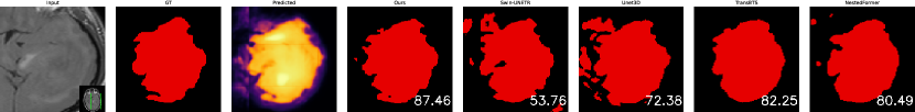
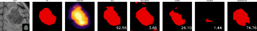
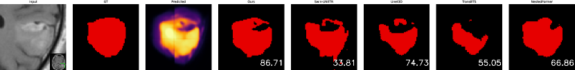
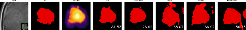
Figure S2: Visualization of predictions of our method and the baselines on the samples from the LGG FLAIR test set. The overlaid numbers are Dice scores.

References

- [1] Asad, M., Dorent, R., Vercauteren, T.: Fastgeodis: Fast generalised geodesic distance transform. arXiv preprint arXiv:2208.00001 (2022)
- [2] Berman, M., Triki, A.R., Blaschko, M.B.: The lovász-softmax loss: A tractable surrogate for the optimization of the intersection-over-union measure in neural networks. In: Proceedings of the IEEE conference on computer vision and pattern recognition. pp. 4413–4421 (2018)
- [3] Bertels, J., Eelbode, T., Berman, M., Vandermeulen, D., Maes, F., Bisschops, R., Blaschko, M.B.: Optimizing the dice score and jaccard index for medical image segmentation: Theory and practice. In: Medical Image Computing and Computer Assisted Intervention–MICCAI 2019: 22nd International Conference, Shenzhen, China, October 13–17, 2019, Proceedings, Part II 22. pp. 92–100. Springer (2019)
- [4] Buda, M., Saha, A., Mazurowski, M.A.: Association of genomic subtypes of lower-grade gliomas with shape features automatically extracted by a deep learning algorithm. Computers in biology and medicine 109, 218–225 (2019)
- [5] Canny, J.: A computational approach to edge detection. IEEE Transactions on pattern analysis and machine intelligence (6), 679–698 (1986)
- [6] Fu, K., Gu, I.Y., Ödblom, A., Liu, F.: Geodesic distance transform-based salient region segmentation for automatic traffic sign recognition. In: 2016 IEEE Intelligent Vehicles Symposium (IV). pp. 948–953. IEEE (2016)
- [7] Hatamizadeh, A., Nath, V., Tang, Y., Yang, D., Roth, H.R., Xu, D.: Swin unetr: Swin transformers for semantic segmentation of brain tumors in mri images. In: International MICCAI Brainlesion Workshop. pp. 272–284. Springer (2021)
- [8] Hatamizadeh, A., Tang, Y., Nath, V., Yang, D., Myronenko, A., Landman, B., Roth, H.R., Xu, D.: Unetr: Transformers for 3d medical image segmentation. In: Proceedings of the IEEE/CVF winter conference on applications of computer vision. pp. 574–584 (2022)
- [9] Kerfoot, E., Clough, J., Oksuz, I., Lee, J., King, A.P., Schnabel, J.A.: Left-ventricle quantification using residual u-net. In: Statistical Atlases and Computational Models of the Heart. Atrial Segmentation and LV Quantification Challenges: 9th International Workshop, STACOM 2018, Held in Conjunction with MICCAI 2018, Granada, Spain, September 16, 2018, Revised Selected Papers 9. pp. 371–380. Springer (2019)
- [10] Lin, T.Y., Goyal, P., Girshick, R., He, K., Dollár, P.: Focal loss for dense object detection. In: Proceedings of the IEEE international conference on computer vision. pp. 2980–2988 (2017)
- [11] Liu, Z., He, X., Lu, Y.: Combining unet 3+ and transformer for left ventricle segmentation via signed distance and focal loss. Applied Sciences 12(18), 9208 (2022)
- [12] Ma, J., Wang, C., Liu, Y., Lin, L., Li, G.: Enhanced soft label for semi-supervised semantic segmentation. In: Proceedings of the IEEE/CVF International Conference on Computer Vision. pp. 1185–1195 (2023)
- [13] Menze, B.H., Jakab, A., Bauer, S., Kalpathy-Cramer, J., Farahani, K., Kirby, J., Burren, Y., Porz, N., Slotboom, J., Wiest, R., et al.: The multimodal brain tumor image segmentation benchmark (brats). IEEE transactions on medical imaging 34(10), 1993–2024 (2014)
- [14] Myronenko, A.: 3d mri brain tumor segmentation using autoencoder regularization. In: Brainlesion: Glioma, Multiple Sclerosis, Stroke and Traumatic Brain Injuries: 4th International Workshop, BrainLes 2018, Held in Conjunction with MICCAI 2018, Granada, Spain, September 16, 2018, Revised Selected Papers, Part II 4. pp. 311–320. Springer (2019)
- [15] Salehi, S.S.M., Erdogmus, D., Gholipour, A.: Tversky loss function for image segmentation using 3d fully convolutional deep networks. In: International workshop on machine learning in medical imaging. pp. 379–387. Springer (2017)
- [16] She, D., Zhang, Y., Zhang, Z., Li, H., Yan, Z., Sun, X.: Eoformer: Edge-oriented transformer for brain tumor segmentation. In: International Conference on Medical Image Computing and Computer-Assisted Intervention. pp. 333–343. Springer (2023)
- [17] Siegel, R.L., Miller, K.D., Fuchs, H.E., Jemal, A.: Cancer statistics, 2022. CA: a cancer journal for clinicians 72(1), 7–33 (2022)
- [18] Szegedy, C., Vanhoucke, V., Ioffe, S., Shlens, J., Wojna, Z.: Rethinking the inception architecture for computer vision. In: Proceedings of the IEEE conference on computer vision and pattern recognition. pp. 2818–2826 (2016)
- [19] Toivanen, P.J.: New geodosic distance transforms for gray-scale images. Pattern Recognition Letters 17(5), 437–450 (1996)
- [20] Vasudeva, S.A., Dolz, J., Lombaert, H.: Geols: Geodesic label smoothing for image segmentation. In: Medical Imaging with Deep Learning. pp. 468–478. PMLR (2024)
- [21] Verduin, M., Compter, I., Steijvers, D., Postma, A.A., Eekers, D.B., Anten, M.M., Ackermans, L., Ter Laan, M., Leijenaar, R.T., van de Weijer, T., et al.: Noninvasive glioblastoma testing: multimodal approach to monitoring and predicting treatment response. Disease markers 2018 (2018)
- [22] Wang, G., Zuluaga, M.A., Li, W., Pratt, R., Patel, P.A., Aertsen, M., Doel, T., David, A.L., Deprest, J., Ourselin, S., et al.: Deepigeos: a deep interactive geodesic framework for medical image segmentation. IEEE transactions on pattern analysis and machine intelligence 41(7), 1559–1572 (2018)
- [23] Wang, W., Chen, C., Ding, M., Yu, H., Zha, S., Li, J.: Transbts: Multimodal brain tumor segmentation using transformer. In: Medical Image Computing and Computer Assisted Intervention–MICCAI 2021: 24th International Conference, Strasbourg, France, September 27–October 1, 2021, Proceedings, Part I 24. pp. 109–119. Springer (2021)
- [24] Wang, Z., Blaschko, M.B.: Jaccard metric losses: Optimizing the jaccard index with soft labels. arXiv preprint arXiv:2302.05666 (2023)
- [25] Wang, Z., Popordanoska, T., Bertels, J., Lemmens, R., Blaschko, M.B.: Dice semimetric losses: Optimizing the dice score with soft labels. arXiv preprint arXiv:2303.16296 (2023)
- [26] Xing, Z., Yu, L., Wan, L., Han, T., Zhu, L.: Nestedformer: Nested modality-aware transformer for brain tumor segmentation. In: International Conference on Medical Image Computing and Computer-Assisted Intervention. pp. 140–150. Springer (2022)
- [27] Xue, Y., Tang, H., Qiao, Z., Gong, G., Yin, Y., Qian, Z., Huang, C., Fan, W., Huang, X.: Shape-aware organ segmentation by predicting signed distance maps. In: Proceedings of the AAAI Conference on Artificial Intelligence. vol. 34, pp. 12565–12572 (2020)
- [28] Zhou, Z., Siddiquee, M.M.R., Tajbakhsh, N., Liang, J.: Unet++: Redesigning skip connections to exploit multiscale features in image segmentation. IEEE transactions on medical imaging 39(6), 1856–1867 (2019)