Variance-Reducing Couplings for Random Features: Perspectives from Optimal Transport

Abstract

Random features (RFs) are a popular technique to scale up kernel methods in machine learning, replacing exact kernel evaluations with stochastic Monte Carlo estimates. They underpin models as diverse as efficient transformers (by approximating attention) to sparse spectrum Gaussian processes (by approximating the covariance function). Efficiency can be further improved by speeding up the convergence of these estimates: a variance reduction problem. We tackle this through the unifying framework of optimal transport, using theoretical insights and numerical algorithms to develop novel, high-performing RF couplings for kernels defined on Euclidean and discrete input spaces. They enjoy concrete theoretical performance guarantees and sometimes provide strong empirical downstream gains, including for scalable approximate inference on graphs. We reach surprising conclusions about the benefits and limitations of variance reduction as a paradigm.

1 Introduction

Kernel methods are ubiquitous in machine learning (Canu and Smola, 2006; Smola and Schölkopf, 2002; Kontorovich et al., 2008; Campbell, 2002). Through the kernel trick, they provide a mathematically principled and elegant way to perform nonlinear inference using linear learning algorithms. The eponymous positive definite kernel function $k:\mathcal{X}\times\mathcal{X}\to\mathbb{R}$ measures the ‘similarity’ between two datapoints. The input domain $\mathcal{X}$ may be continuous, e.g. the set of vectors in $\mathbb{R}^{d},$ or discrete, e.g. the set of graph nodes or entire graphs.

Random features for kernel approximation. Though very effective on small datasets, kernel methods suffer from poor scalability. The need to materialise and invert the Gram matrix $\mathbf{K}\coloneqq[k(\bm{x}_{i},\bm{x}_{j})]_{i=1}^{N}$ leads to a time complexity cubic in the size of the dataset $N$. Substantial research has been dedicated to improving scalability by approximating this matrix, a prominent example being random features (RFs) (Rahimi and Recht, 2007, 2008; Avron et al., 2017b; Liu et al., 2022). These randomised mappings $\phi:\mathbb{R}^{d}\to\mathbb{R}^{s}$ construct low-dimensional or sparse feature vectors that satisfy

$$k(\bm{x},\bm{y})=\mathbb{E}\left(\phi(\bm{x})^{\top}\phi(\bm{y})\right).$$ (1)

The features $\phi(\bm{x})$ are typically constructed using ensembles of random frequencies $\{\bm{\omega}\}_{i=1}^{m}$ drawn from some known distribution $\mathcal{\eta}$. The choice of $\eta$ and manner in which they are combined to construct $\phi(\bm{x})$ depends on the particular input space $\mathcal{X}$ and kernel function $k$ being approximated. The set of RFs $\{\phi(\bm{x}_{i}\}_{i=1}^{N}$ can then be used to construct a low-rank or sparse approximation of the Gram matrix, providing substantial space and time complexity savings. RFs exist for a variety of kernels, including for continuous and discrete input spaces (Dasgupta et al., 2010; Johnson, 1984; Choromanski et al., 2020; Goemans and Williamson, 2001; Rahimi and Recht, 2007; Choromanski, 2023).

Variance reduction for RFs. Eq. 1 can be understood as a Monte Carlo (MC) estimate of $k$. In practical applications, it is often found that this estimate converges slowly. This can be addressed by taking many features $m$, but this undermines the efficiency gains of RFs. Therefore, substantial effort has been dedicated to reducing the variance of the kernel estimates. Variance reduction methods include quasi-Monte Carlo (QMC) (Dick et al., 2013; Yang et al., 2014a), common random numbers (CRNs) (Glasserman and Yao, 1992), antithetic variates (Hammersley and Morton, 1956) and structured Monte Carlo (SMC) (Yu et al., 2016), all of which are well-studied in computational statistics. These techniques all ultimately work by replacing i.i.d. frequencies $\{\bm{\omega}_{i}\}_{i=1}^{m}$ by a dependent ensemble, with the dependencies between samples designed to improve RF convergence.

Limitations of previous techniques. The best choice of dependencies between $\{\bm{\omega}_{i}\}_{i=1}^{m}$ is an active research area. Though straightforward to apply, standard QMC techniques are suboptimal. They are based on fixed ‘low-discrepancy sequences’ so typically do not incorporate information about the particular kernel function $k$ being approximated. Empirical performance may be poor and theoretical guarantees lacking in the low-sample, high-dimensional regime (Rowland et al., 2018; Morokoff and Caflisch, 1995) – which is precisely where RFs are most important. On the other hand, hand-crafted SMC dependencies – which impose strict geometrical conditions like orthogonality between frequencies – tend to fare better (Yu et al., 2016). But they are still difficult to design, theoretical guarantees are hard-won and optimality is not guaranteed. RFs for estimating kernels defined on discrete spaces like the nodes of a graph have only recently been developed (Choromanski, 2023; Tripp et al., 2024), so here very few effective variance reduction techniques have even been proposed.

Optimal transport. To address these shortcomings, we propose to frame variance reduction as optimal transport: an active research area of applied mathematics that studies how to move (probability) mass between distributions as efficiently as possible (Villani et al., 2009). This fruitful perspective equips us with proof techniques and numerical tools to identify the best possible dependencies between samples, giving lower kernel estimator variance compared to previous approaches. We use these insights to develop better couplings for RFs in Euclidean and discrete spaces.

Our contributions. We summarise our key contributions below.

1. We frame the problem of variance reduction of RFs as optimal transport (OT) (Sec. 2), and use this perspective to improve the convergence of three popular classes of RFs: random Fourier features, random Laplace features and graph random features.

2. For random Fourier features (RFFs) and random Laplace features (RLFs), we exactly solve the OT problem for the norms of $m=2$ orthogonal frequencies, finding a novel coupling with the lowest possible variance (Sec. 3). We use a copula as a numerical OT solver to consider arbitrary $m$.

3. For graph random features (GRFs), we couple the lengths of random walks by solving an OT bipartite matching, outcompeting previous algorithms for estimating graph node kernels (Sec. 4).

4. We test our algorithms on UCI datasets and real-world graphs, verifying that OT couplings substantially reduce kernel estimator variance (Secs 3 and 4). We show that this sometimes translates to much better performance in downstream tasks (in particular, approximate inference with scalable graph-based Gaussian processes), but also reach surprising conclusions about the limitations of variance reduction for RFs in machine learning.

All proofs are saved for the Appendices, but are also sketched in the main body where space allows. We will make source code available if accepted.

2 Background

From kernel estimation to optimal transport (OT). Considering the expression in Eq. 1, define the kernel estimator $\widehat{k}(\bm{x}_{i},\bm{x}_{j})\coloneqq\phi(\bm{x}_{i})^{\top}\phi(\bm{x}_{j})$. Recall that $\phi(\cdot)$ is computed using random frequencies $\{\bm{\omega}_{i}\}_{i=1}^{m}$, with the space in which they live, distribution from which they are drawn, and manner in which they are combined dependent on the particular kernel being approximated. The estimator is unbiased provided each frequency $\bm{\omega}_{i}$ obeys some known, fixed marginal distribution $\eta$. Importantly, independence of $\{\bm{\omega}_{i}\}_{i=1}^{m}$ is not a requirement: any joint distribution with marginals $\eta$ gives an unbiased estimator. We refer to the set of such joint distributions as couplings.

The choice of coupling between the $m$ frequencies determines the variance of the estimator. It is straightforward to see that finding the coupling $\mu^{*}$ that minimises this variance is equivalent to solving

$$\mu^{*}=\textrm{arg inf}_{\mu\in\Lambda_{m}(\eta)}\left[\mathbb{E}_{\bm{\omega}_{1:m}\sim\mu}c(\bm{\omega}_{1:m})\right]$$ (2)

where we defined the cost function

$$c(\bm{\omega}_{1:m})\coloneqq\left(\phi(\bm{x})^{\top}\phi(\bm{y})\right)^{2}.$$ (3)

$\Lambda_{m}(\eta)$ denotes the set of couplings over $m$ random variables with marginal measures $\eta$. This is precisely the Kantorovich formulation of a multi-marginal optimal transport problem, with cost function $c$ (see e.g. Eq. 4 of the seminal OT text of Villani (2021)). The relationship between variance reduction and optimal transport was also noted by Rowland et al. (2018), but in the different setting of estimating the expected value of functions drawn from Gaussian processes.

(Approximately) solving the OT problem. For many popular RF constructions, the OT problem in Eq. 2 is intractable. The cost function and corresponding optimal coupling will in general depend on the choice of RF map and data distribution. A further practical consideration is that, to be useful, $\mu^{*}$ must be easy to sample from; even if it guarantees lower variance, an expensive sampling mechanism will obviate any efficiency gains from a coupling. However, we will see that for certain RFs under particular assumptions we can solve the OT problem exactly, obtaining computationally lightweight couplings that provide the smallest possible kernel estimator variance. Even if the OT problem is intractable, we can often leverage numerical methods to approximately solve Eq. 2. The formulation of these methods will depend on the input domain of the RF being considered.

Remainder of the manuscript. We will demonstrate how insights and algorithms from OT can be used to improve the convergence of RFFs and RLFs (Sec. 3) and GRFs (Sec. 4). These have input domains $\mathcal{X}=\mathbb{R}^{d}$ ($d$-dimensional Euclidean space) and $\mathcal{X}=\mathcal{N}$ (the set of graph nodes), respectively.

3 Random Fourier features and random Laplace features

RFFs and RLFs. To begin, we consider the task of approximating the popular Gaussian kernel $k(\bm{x}_{i},\bm{x}_{j})\coloneqq\exp(-\|\bm{x}_{i}-\bm{x}_{j}\|^{2}/2)$ with data $\{\bm{x}_{i}\}_{i=1}^{N}\subset\mathbb{R}^{d}$. This can be achieved using Rahimi and Recht’s celebrated random Fourier features (RFFs) (Rahimi and Recht, 2007),

$$\phi_{\textrm{RFF}}(\bm{x})=\sqrt{\frac{1}{m}}\left(\odot_{i=1}^{m}\left[\sin(\bm{\omega}_{i}^{\top}\bm{x}),\cos(\bm{\omega}_{i}^{\top}\bm{x})\right]\right),$$ (4)

where $\odot$ denotes concatenation. These provide an unbiased estimate if the frequencies $\{\bm{\omega}_{i}\}_{i=1}^{m}$ are marginally Gaussian, $\bm{\omega}_{i}\sim\mathcal{N}(0,\mathbf{I}_{d})$. They are widely used for scaling kernel methods such as Gaussian processes (GPs; Williams and Rasmussen, 2006) and support vector machines (SVMs; Scholkopf and Smola, 2018). The time complexity of computing the exact posterior of a GP is $\mathcal{O}(N^{3}),$ where $N$ is the number of datapoints. Using RFFs, one can approximate the posterior with $m\ll N$ features, reducing this cost to $\mathcal{O}(Nm^{2})$. Beyond RFFs, $k(\bm{x}_{i},\bm{x}_{j})$ can also be approximated using random Laplace features (RLFs) (Yang et al., 2014b),

$$\phi_{\textrm{RLF}}(\bm{x})=\sqrt{\frac{1}{m}}\exp(-\|\bm{x}\|^{2})(\odot_{i=1}^{m}\exp(\bm{\omega}_{i}^{\top}\bm{x})),$$ (5)

where again $\bm{\omega}_{i}\sim\mathcal{N}(0,\mathbf{I}_{d}).$ Unlike RFFs, RLFs give strictly positive kernel estimates. This makes them better suited to estimating attention in linear-attention transformers (Choromanski et al., 2020), where negative estimates can cause training instabilities. Using $m$ RLFs to write a low-rank decomposition of the attention matrix with $N$ $d$-dimensional tokens, one can reduce the computational cost of transformers from $\mathcal{O}(N^{2}+Nd)$ down to $\mathcal{O}(Nmd)$ with low performance loss.

Orthogonal random features. A common variance reduction technique for both RFFs and RLFs is the orthogonality trick (Yu et al., 2016; Rowland et al., 2018; Reid et al., 2023; Choromanski et al., 2018). Exploiting the isotropy of $\mathcal{N}(0,\mathbf{I}_{d})$, it is possible to constrain the frequency vectors $\{\bm{\omega}_{i}\}_{i=1}^{m}$ to be exactly orthogonal whilst preserving their marginal distributions. This is found to reduce the kernel estimator variance and improve performance in downstream tasks. Whilst this technique couples the directions of the random frequencies $\{\widehat{\bm{\omega}}_{i}\}_{i=1}^{m}$, their norms $\{\omega_{i}\}_{i=1}^{m}$ (with $\omega_{i}\coloneqq\|\bm{\omega}_{i}\|$) are left independent so the coupling is suboptimal. We will now use tools from OT to find a coupling between frequency vector norms that provides strictly lower kernel estimator variance.

3.1 Solving the OT problem for maximal variance reduction

Consider an ensemble of $m$ orthogonal random frequency directions $\{\widehat{\bm{\omega}}_{i}\}_{i=1}^{m}$, jointly randomly rotated so they are marginally isotropic. Recall that our task is to couple their norms $\{\omega_{i}\}_{i=1}^{m}$ to suppress the RFF and RLF kernel estimator variance. The marginal distribution of each $\omega_{i}$ must be $\chi_{d}$ (a Chi distribution with $d$ degrees of freedom) to ensure that each $\bm{\omega}_{i}$ is marginally Gaussian. It is simple to extend recently-derived results (Reid et al., 2023) to compute the OT cost functions.

Lemma 3.1 (OT formulation for RFFs and RLFs).

When estimating $k(\bm{x},\bm{y})$ with $m$ orthogonal RFFs and RLFs, the OT formulation of the variance reduction problem is:

$$\mu^{*}=\arg\inf_{\mu\in\Lambda_{m}(\chi_{d})}\left[\mathbb{E}_{\omega_{1:m}\sim\mu}c(\omega_{1:m})\right],\quad\textrm{where}$$ (6)

$$c_{\textrm{RFF}}(\omega_{1:m})=\sum_{i,j\neq i}^{m}\sum_{k=0}^{\infty}\frac{(-1)^{k}z^{2k}\left(\omega_{i}^{2}+\omega_{j}^{2}\right)^{k}}{2^{2k}k!\Gamma(k+\frac{d}{2})},\quad c_{\textrm{RLF}}(\omega_{1:m})=\sum_{i,j\neq i}^{m}\sum_{k=0}^{\infty}\frac{v^{2k}(\omega_{i}^{2}+\omega_{j}^{2})^{k}}{2^{2k}k!\Gamma(k+\frac{d}{2})},$$ (7)

with $z\coloneqq\|\bm{x}-\bm{y}\|_{2}$ and $v\coloneqq\|\bm{x}+\bm{y}\|_{2}$.

This is a challenging multi-marginal OT problem. However, remarkably, we can solve it exactly, under mild asymptotic assumptions for RFFs, when $m=2$. The following result is novel.

Theorem 3.2 (Solution to OT problem when $m=2$).

Denote by $F_{\chi_{d}}(\cdot)$ the cumulative distribution function (CDF) of $\chi_{d}$. Considering $m=2$ orthogonal frequencies with norms $(\omega_{1},\omega_{2})$, the OT problem in Eq. 6 is solved by the negative monotone coupling

$$F_{\chi_{d}}(\omega_{1})+F_{\chi_{d}}(\omega_{2})=1,$$ (8)

when $\frac{z^{2}}{d}\to 0$ for RFFs and in full generality for RLFs.

Proof sketch. We defer a full proof of this important result to App. A.2, but provide a sketch for the interested reader. It is well known that optimal transport plans satisfy a property called ‘$c$-monotonicity’, which specifies how the support of the optimal coupling depends on the cost function. For $c_{\textrm{RFF}}$ and $c_{\textrm{RLF}}$, we can show that this is commensurate with negative monotonicity (Eq. 8), though only asymptotically for the former. ∎

Given $m=d$ orthogonal frequencies, it is possible to partition the ensemble into $\lfloor\frac{d}{2}\rfloor$ orthogonal pairs, with one remaining frequency if $d$ is odd. For every such pair, we can impose negative monotone coupling (Eq. 8). We refer to such dependent ensembles as pairwise norm-coupled (PNC).

To reduce the variance further, one can of course take multiple independent PNC ensembles. A corollary of Thm. 3.2 is as follows.

Corollary 3.4 (Supriority of pairwise norm-coupled RFs).

The kernel estimator variance with pairwise norm-coupled RFs is strictly lower than orthogonal RFs with independent norms, provided $\frac{z^{2}}{d}\to 0$ for RFFs and in full generality for RLFs.

Negative monotone coupling differs from OT plans usually seen in machine learning; it is a space-filling coupling that seeks long transport plans that give diverse samples. However, it is a popular heuristic technique for variance reduction via common random numbers (CRNs) in computational statistics (Glasserman and Yao, 1992). This is (to our knowledge) the first result applying it to improving the convergence of orthogonal RFs, and the first corresponding guarantees for variance reduction. We make one further theoretical contribution regarding coupled RLFs.

Theorem 3.5 (Recovering antithetic sampling with RLFs).

For RLFs with $m=2$ frequencies whose respective orientations $(\widehat{\bm{\omega}}_{1},\widehat{\bm{\omega}}_{2})$ are unconstrained, the variance reduction OT problem is solved by conditioning that $\bm{\omega}_{1}=-\bm{\omega}_{2}$ almost surely (that is, opposite directions and equal norms).

This coupling is popularly known as antithetic sampling (Hammersley and Morton, 1956). Thm. 3.5 shows that, given a PNC ensemble $\{\bm{\omega}_{i}\}_{i=1}^{d}$, we can obtain further variance reduction by augmenting it to $\{\pm\bm{\omega}_{i}\}_{i=1}^{d}$. Antithetic sampling is also a common (though often heuristically motivated) variance reduction strategy used e.g. when estimating attention in Performers (Choromanski et al., 2020). We can reinterpret its effectiveness through the lens of OT. Note that Thm. 3.5 does not hold for RFFs.

3.2 Pushing further with numerical OT solvers

Multi-marginal OT. The insights of Sec. 3.1 have equipped us with pairwise norm-coupled RFs: a computationally efficient coupling that guarantees strictly lower kernel estimator variance. We obtained it by solving the variance reduction OT problem exactly in $m=2$, then combining $\lfloor\frac{d}{2}\rfloor$ independent copies of such pairs to get the ensemble. A natural question is whether we can do better by inducing dependencies between the all the $d$ frequencies’ norms. Solving this multi-marginal optimal transport problem analytically is a challenging open problem.

Copulas as numerical OT solvers. Whilst a full analytic solution to the multi-marginal OT variance-reduction problem is (for now) out of reach, we can make progress using a numerical OT solver. Our basic strategy is to restrict $\Lambda_{m}(\chi_{d})$, the full set of joint distributions over $m$ random variables with $\chi_{d}$ marginals, to a tractable subset amongst which we can efficiently optimise and sample. One such subset is provided by Gaussian copulas (Nelsen, 2006; Haugh, 2016): joint distributions obtained by taking a multivariate Gaussian and pushing each of its coordinates forward first with the Gaussian CDF $F_{\mathcal{N}}$, and then the $\chi_{d}$ inverse CDF $F_{\chi_{d}}^{-1}$. If the diagonal terms of the underlying Gaussian covariance matrix $\mathbf{\Sigma}\in\mathbb{R}^{m\times m}$ are equal to $1$ (i.e. it is a correlation matrix), this has the prescribed marginals so unbiasedness is baked in. Meanwhile, correlations between the random variables are controlled by the off-diagonal entries of $\mathbf{\Sigma}$. This family parameterises a very broad (though not universal) set of couplings, including pairwise norm-coupled RFs (Def. 3.3).

In App. A.5 we show that it is possible to use gradient descent with the reparameterisation trick to learn the optimal copula covariance matrix $\mathbf{\Sigma}$, approximately solving the multi-marginal OT problem (Chi et al., 2019). We do this by minimising the kernel approximation error on training data, exploiting the fact that all operations to construct the features are differentiable. Remarkably, optimising the copula recovers our pairwise norm-coupling scheme (or other equally well-performing variants). This suggests that PNC may in fact exactly solve the multi-marginal OT problem in Eq. 6, a tantalising possibility which we aim to explore in future work.

3.3 Experiments for norm-coupled RFs

Fourier Features	Concrete	Abalone	CPU	Power	Airfoil	Boston
i.i.d.	$1.000$ $\pm 0.028$	$1.000$ $\pm 0.042$	$1.000$ $\pm 0.082$	$1.000$ $\pm 0.037$	$1.000$ $\pm 0.023$	$1.000$ $\pm 0.018$
Halton	$1.028$ $\pm 0.029$	$0.991$ $\pm 0.042$	$0.995$ $\pm 0.082$	$0.913$ $\pm 0.033$	$0.927$ $\pm 0.021$	$1.176$ $\pm 0.022$
Orthogonal	$0.627$ $\pm 0.019$	$0.535$ $\pm 0.023$	$0.617$ $\pm 0.070$	$0.669$ $\pm 0.024$	$0.586$ $\pm 0.013$	$0.639$ $\pm 0.016$
+ PNC	$\mathbf{0.563}$ $\pm 0.019$	$\mathbf{0.433}$ $\pm 0.019$	$\mathbf{0.544}$ $\pm 0.071$	$\mathbf{0.547}$ $\pm 0.020$	$\mathbf{0.481}$ $\pm 0.011$	$\mathbf{0.606}$ $\pm 0.018$
Laplace Features	Concrete	Abalone	CPU	Power	Airfoil	Boston
i.i.d.	$1.000$ $\pm 0.092$	$1.000$ $\pm 0.036$	$1.000$ $\pm 0.086$	$1.000$ $\pm 0.018$	$1.000$ $\pm 0.026$	$1.000$ $\pm 0.029$
Halton	$0.721$ $\pm 0.067$	$0.777$ $\pm 0.031$	$0.779$ $\pm 0.084$	$0.728$ $\pm 0.015$	$0.721$ $\pm 0.021$	$0.893$ $\pm 0.028$
Orthogonal	$0.418$ $\pm 0.041$	$0.546$ $\pm 0.026$	$\mathbf{0.614}$ $\pm 0.098$	$0.527$ $\pm 0.013$	$0.489$ $\pm 0.016$	$0.360$ $\pm 0.019$
+ PNC + antithetic	$\mathbf{0.367}$ $\pm 0.043$	$\mathbf{0.486}$ $\pm 0.027$	$\mathbf{0.618}$ $\pm 0.119$	$\mathbf{0.438}$ $\pm 0.013$	$\mathbf{0.418}$ $\pm 0.016$	$\mathbf{0.324}$ $\pm 0.019$

Table 1: Performance of RFFs and RLFs on kernel estimation with UCI datasets with different coupling schemes, taking $d$ random frequencies for RFFs and $2d$ for RLFs (see main text for details). We show RMSEs to the ground truth kernel values, normalised such that the RMSE of the i.i.d. estimator is equal to one. Lower is better. Error bars are standard errors on the reported RMSEs.

To verify the efficacy of pairwise norm-coupled RFs (Def. 3.3), we now compute kernel estimates with RFFs and RLFs for real-world UCI datasets. We choose the kernel lengthscale parameters (equivalently, the data normalisation) based on a training set, either by training a GP (RFFs) or selecting reasonable values for downstream Performer applications (RLFs) (Choromanski et al., 2020). We then compute the kernel approximation RMSE on a test set. Full details are in App. B.1.

Results. Table 1 shows the results. For RFFs, we take $m=d$ orthogonal frequencies. For RLFs, we also include their antiparallel directions, giving $m=2d$ frequencies. For each dataset, the RMSEs are normalised by the result with i.i.d. features. As a further baseline, we include RFs constructed using Halton sequences (Dick et al., 2013; Yang et al., 2014a), a fixed, off-the-shelf QMC scheme that sometimes provides gains but is clearly suboptimal. The third row shows orthogonal frequencies with independent norms (Yu et al., 2016). When we also couple the frequencies’ norms using our OT-driven PNC scheme (plus antithetic sampling for RLFs, due to Thm 3.5), we access even lower estimator variance at no extra computational cost. Note that the $z^{2}/d\to 0$ condition for RFFs is found to be nonrestrictive, and coincides with the $d\to\infty$ limit where standard QMC may fail.

Downstream tasks. We have achieved our objective of variance reduction, a popular goal in the literature (Yu et al., 2016; Lyu, 2017). One might therefore expect PNC RFs to improve downstream performance. We do not observe this (see App. B.2): a surprising observation we return to in Sec. 5.

4 Graph random features

We now shift our attention from $\mathbb{R}^{d}$ to the discrete domain. Consider an undirected graph $\mathcal{G}(\mathcal{N},\mathcal{E})$ where $\mathcal{N}\coloneqq\{v_{1},...,v_{N}\}$ is the set of nodes and $\mathcal{E}$ is the set of edges, with $(v_{i},v_{j})\in\mathcal{E}$ if and only if there exists an edge between $v_{i}$ and $v_{j}$ in $\mathcal{G}$. Graph node kernels $k:\mathcal{N}\times\mathcal{N}\to\mathbb{R}$ are positive definite, symmetric functions defined on pairs of nodes of $\mathcal{G}$, reflecting some notion of their ‘closeness’ via the graph edges and weights. $k$ captures the structure of $\mathcal{G}$, letting practitioners repurpose popular kernelised learning algorithms – including their theoretical guarantees and empirical success – to the discrete domain (Smola and Kondor, 2003b, a). Examples include the diffusion, regularised Laplacian, cosine and random walk kernels, all of which are typically considered as functions of the graph Laplacian matrix (Kondor and Lafferty, 2002). We give a short introduction in App. C.1.

Graph random features. As in the Euclidean setting, graph-based kernel methods scale notoriously poorly on account of the $\mathcal{O}(N^{3})$ time complexity of inverting the Gram matrix $\mathbf{K}\coloneqq[k(v_{i},v_{j})]_{i,j=1}^{N}$. In fact, even computing $\mathbf{K}$ often incurs a cubic cost since it involves multiplying large adjacency matrices. This has motivated research dedicated to improving efficiency by approximating $\mathbf{K}$, including the recently-introduced class of graph random features (GRFs) (Choromanski, 2023; Reid et al., 2024b). These are finite-dimensional, explicitly manifested vectors $\{\phi_{\textrm{GRF}}(v_{i})\}_{i=1}^{N}\subset\mathbb{R}^{N}$ whose Euclidean dot product is equal to the graph kernel evaluation in expectation,

$$\mathbf{K}_{ij}=\mathbb{E}\left[\phi_{\textrm{GRF}}(v_{i})^{\top}\phi_{\textrm{GRF}}(v_{j})\right].$$ (9)

GRFs enable practitioners to compute a sparse, unbiased estimate of the graph kernel (or its inverse) in subquadratic time. They can be constructed for arbitrary functions of a weighted adjacency matrix.

Coupled random walks. Whereas RFFs and RLFs sample random vectors in $\mathbb{R}^{d}$, GRFs sample simple random walks. These are sequences of graph nodes $(v_{i})_{i=1}^{l}$ where consecutive nodes are connected by an edge, $(v_{i},v_{i+1})\in\mathcal{E}$. At every timestep, the walker chooses one of its neighbours uniformly and at random. The length of the walk $l$ may itself be a random variable. For GRFs, it is drawn from a geometric distribution $l\sim\textrm{G}(p),p\in(0,1)$, which corresponds to the walker terminating with probability $p$ at every timestep.

Random walks are usually taken to be independent, but this can lead to slow mixing times, poor efficiency and high kernel estimator variance (Alon et al., 2007; Zhou et al., 2015). A natural question is: can we use insights from OT to couple graph random walks to improve the convergence of GRFs?

The simplest approach to induce dependencies between random walks is to couple their lengths. For GRFs, the constraint for unbiasedness is that the marginal distribution of each random variable $l$ must remain geometric. Reid et al. (2024c) recently proposed a simple, heuristically-motivated algorithm to achieve this called antithetic termination, which directly anticorrelates the termination events between walkers at every timestep (see App. C.2). They provide asymptotic theoretical guarantees, but only for particular choices of graph kernel. In the following section, we will see that an OT-based approach that optimises a coupling using real data performs substantially better.

4.1 Approximating and solving the OT problem for GRFs

Here, we present our approach for formulating and approximately solving the variance reduction OT problem with GRFs. It works by mapping to a corresponding bipartite matching problem which we can solve efficiently.

Constructing GRFs from random walks. GRFs are constructed differently to RFFs and RLFs. To obtain $\phi_{\textrm{GRF}}(v_{i})\in\mathbb{R}^{N}$ (where $v_{i}\in\mathcal{N}$), we sample $m$ random walks $\{\bm{\omega}_{k}^{(i)}\}_{k=1}^{m}$ out of node $v_{i}$ and compute the arithmetic mean of their corresponding ‘projections’,

$$\phi_{\textrm{GRF}}(v_{i})=\frac{1}{m}\sum_{k=1}^{m}\psi(\bm{\omega}_{k}^{(i)}).$$ (10)

Here, the projection function $\psi(\cdot):\Omega\to\mathbb{R}^{N}$ maps from the set of graph random walks $\Omega\coloneqq\left\{(v_{i})_{i=1}^{l}\,|\,v_{i}\in\mathcal{N},(v_{i},v_{i+1})\in\mathcal{E},l\in\mathbb{N}\right\}$ to a sparse $N$-dimensional feature vector satisfying $k(v_{i},v_{j})=\mathbb{E}_{\bm{\omega}^{(i)},\bm{\omega}^{(j)}}[\psi(\bm{\omega}^{(i)})^{\top}\psi(\bm{\omega}^{(j)})]$. $\psi(\cdot)$ depends on the particular kernel being approximated. We refer the reader to the works of Choromanski (2023) and Reid et al. (2024b) for an introduction to GRFs, but also provide background in App. C.1 for completeness. For our purposes, it will be sufficient to note that $\psi(\cdot)$ is a complicated function; it is difficult to reason about analytically but straightforward to compute for a particular walk. Moreover, its input walks are discrete random variables so $\psi(\cdot)$ is not differentiable with respect to their lengths $l_{k}^{(i)}$ (where $k=1,...,m$ and $v_{i}\in\mathcal{N}$ is the walker’s start node) – a property that will preclude optimisation using copulas (Sec. 3.2).

A pair of walkers. Let us initially consider just $m=2$ walkers. The kernel estimator $\widehat{k}(v_{i},v_{j})$ is

$$\widehat{k}(v_{i},v_{j})=\phi_{\textrm{GRF}}(v_{i})^{\top}\phi_{\textrm{GRF}}(v_{j})=\frac{1}{4}\left(\psi(\bm{\omega}_{1}^{(i)})+\psi(\bm{\omega}_{2}^{(i)})\right)^{\top}\left(\psi(\bm{\omega}_{1}^{(j)})+\psi(\bm{\omega}_{2}^{(j)})\right),$$ (11)

which is unbiased provided (i) the marginal distribution of each $\bm{\omega}_{1,2}^{(i,j)}$ is a simple random walk with geometrically distributed length (hereafter denoted $\eta_{\textrm{G}}$) and (ii) walks from node $v_{i}$ are independent from walks from node $v_{j}$. The variance of the estimator depends on the quantity

$$\mathbb{E}\left(\widehat{k}(v_{i},v_{j})^{2}\right)=\frac{1}{4}\mathbb{E}_{\bm{\omega}_{1,2}^{(i,j)}}\left[\left(\psi(\bm{\omega}_{1}^{(i)})+\psi(\bm{\omega}_{2}^{(i)})\right)^{\top}\left(\psi(\bm{\omega}_{1}^{(j)})+\psi(\bm{\omega}_{2}^{(j)})\right)\right]^{2},$$ (12)

where the expectation is taken over both the directions and lengths of the random walks. Suppose the directions remain independent, but the lengths $l_{1}^{(i)}$ and $l_{2}^{(i)}$ (and likewise $l_{1}^{(j)}$ and $l_{2}^{(j)}$) are to be coupled for variance reduction. The OT problem can then be written

$$\mu^{*}=\arg\inf_{\mu\in\Lambda_{2}(\eta_{\textrm{G}})}\mathbb{E}_{(l_{1}^{(i)},l_{2}^{(i)})\sim\mu,(l_{1}^{(j)},l_{2}^{(j)})\sim\mu}\left(\mathbb{E}_{\textrm{dirs}}\left[\left(\psi(\bm{\omega}_{1}^{(i)})+\psi(\bm{\omega}_{2}^{(i)})\right)^{\top}\left(\psi(\bm{\omega}_{1}^{(j)})+\psi(\bm{\omega}_{2}^{(j)})\right)\right]^{2}\right),$$ (13)

where $\mathbb{E}_{\textrm{dirs}}$ denotes the expectation over the walkers’ directions, i.e. which neighbour they choose at each timestep.

OT, permutation densities and bipartite matchings. The OT problem in Eq. 13 is analytically intractable. To make progress, we must make some approximations. We report them in full in App. C.3; Fig. 6 provides a visual overview. We limit the main text to the most important points.

Our first problem is intractability of the cost function in Eq. 13. We can mitigate this by moving $\mathbb{E}_{\textrm{dirs}}$, the expectation over walker directions, inside the square brackets. This clearly modifies the objective, ignoring higher-order correlations between features induced by walker directions (but not lengths). However, it yields a cost function we can estimate efficiently, if not compute exactly.

The second challenge is optimising over the class of couplings $\Lambda_{2}(\eta_{\textrm{G}})$, joint distributions over two discrete random variables with geometrically distributed marginals. As in Sec. 3.2, a sensible numerical approach is to optimise amongst a tractable subclass of $\Lambda_{2}(\eta_{\textrm{G}})$. Copulas are unsuitable because in this discrete setting we cannot compute gradients to optimise the covariance matrix. Instead, we consider the family of measures $\pi^{(\sigma)}$ on $[0,1]^{2}$ described by the permutation densities

$$p_{\sigma}(x,y)\coloneqq n1_{\sigma(\lceil nx\rceil)=\lceil ny\rceil},$$ (14)

with $\sigma$ a permutation of order $n$ (that is, a bijection $\sigma:[\![n]\!]\to[\![n]\!]$). The unit square is split into a $n\times n$ grid where each row and column has a single ‘tile’ of probability density $n$ and is $0$ otherwise.

Note that both marginal distributions of $\pi^{(\sigma)}$ are manifestly uniform on $[0,1]$. Moreover, the marginals can be transformed to an arbitrary probability distribution $\eta$ by pushing forward with the inverse CDF, $F_{\eta}^{-1}(\cdot)\coloneqq\inf\{x\in\mathbb{R}:F_{\eta}(x)\geq\cdot\}$. Transforming both coordinates in this way yields a joint measure $\mu^{(\sigma)}\in\Lambda_{2}(\eta)$ which will give an unbiased estimator. We will refer to these as $\sigma$-couplings, and remark that $n!$ such couplings exist for a given permutation order $n$.

The permutations $\sigma\in S_{n}$ can be interpreted as matchings between the $n$ quantiles of the geometric distributions over the lengths of a pair of walkers. With the right choice of $\sigma$, they can ensure that e.g. if one of the walk lengths is short then the other tends to be long, diversifying the ensemble. In App. C.1 we formalise this by writing the optimisation of $\sigma$ as a bipartite matching problem, with a cost matrix estimated by sampling walks. Unfortunately, the matching problem has quadratic weights (albeit with some extra symmetric structure). It is challenging; we discuss progress towards a fast, exact algorithm in App. C.3.1. More pragmatically, with another simplification we can obtain a related linear-weights bipartite matching problem. This can be solved efficiently in time $\mathcal{O}(n^{3})$ using linear programming techniques, e.g. the Hungarian algorithm (Kuhn, 1955), thereby optimising the coupling $\mu^{(\sigma)}$. Taking the optimal permutation $\sigma$, we define $\sigma$-coupled GRFs as follows.

Besides being easy to optimise and sample from, there are also more rigorous OT motivations for the choice of $\sigma$-couplings $\mu^{(\sigma)}$. They relate to the asymptotic behaviour of $\mu^{(\sigma)}$ as the permutation order $n\to\infty$ and the stability of OT plans (Villani, 2021). We defer this technical point to App. D.

As in Sec. 3.2, an interesting question is whether one could couple the lengths of $m>2$ walkers. This is challenging and has received little attention in the literature. One possibility would be to combine $m-1$ permutations, finding a minimum-weights $m$-partite matching with all subgraphs constrained to be complete $K_{m}$. Another approach would be to approximately solve this multi-marginal OT problem using the Sinkhorn-Knopp algorithm (Sinkhorn and Knopp, 1967; Cuturi, 2013).

Broader applicability. As a final remark, the utility of our OT-approach to coupling walker lengths extends to graph-based estimators beyond GRFs. For example, it can be used to improve estimates of the PageRank vector, a popular measure of the relative importance of the nodes $\mathcal{N}$ of a graph proposed by Page et al. (1998) to rank websites in search engine results. We discuss this in App. E.

4.2 Experiments with $\sigma$-coupled GRFs

In this section, we empirically evaluate $\sigma$-coupled GRFs for variance reduction of graph node kernel estimates. We begin by testing our method on a variety of real-world graphs, then show that lower variance unlocks better approximate inference with scalable graph-based Gaussian processes (GPs).

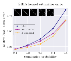
Figure 1: Kernel estimator error vs termination probability. Insets show permutations for $p\in\{0.1,0.2,0.3,0.4,0.5\}$.

Gram matrix approximation. GRFs take the termination probability $p$ as a hyperparameter, determining the rate of decay of the geometric distribution over walk length. A smaller value of $p$ samples longer walks and gives more accurate kernel estimates, but takes longer to run. The optimal coupling changes depending on $p$. We will consider the values $p\in\{0.1,0.2,0.3,0.4,0.5\}$, finding the optimal permutation $\sigma$ in each case.

To find the optimal $\sigma$, we solve the matching problem (App. C.3) for a random Erdős-Rényi graph with $N=100$ nodes, taking a permutation order $n=30$ and choosing the $2$-regularised Laplacian kernel as our target. We then use the Hungarian algorithm, averaging the cost matrix over every possible node pair $(v_{i},v_{j})\in\mathcal{N}^{2}$ to find a coupling that reduces the variance of all entries of the Gram matrix.

Having computed couplings $\mu^{(\sigma)}$ for each value of $p$, we then test the corresponding $\sigma$-coupled GRFs on a variety of real-world graphs. Fig. 1 shows the results for cora ($N=2708$), with the rest left to App. F.1. We plot the relative Frobenius norm error of the Gram matrix approximation $\|\mathbf{K}-\widehat{\mathbf{K}}\|_{\textrm{F}}/\|\mathbf{K}\|_{\textrm{F}}$ with walkers that are i.i.d., antithetic (Reid et al., 2024c) or $\sigma$-coupled. For every value of $p$, $\sigma$-coupled GRFs give equally good or smaller kernel estimator errors. Our general-purpose OT approach often substantially outperforms antithetic termination: a bespoke algorithm designed specifically to improve GRFs. We include visualisations of the optimal permutations for different values of $p$ in the inset, verifying that the $\sigma$-coupling adapts to different GRF hyperparamaters.

Novel application: $\sigma$-coupled GRFs for scalable graph-based GPs. We conclude this section by applying $\sigma$-coupled GRFs to scalable graph-based Gaussian processes (GPs), where we find that the improved estimation of the covariance function permits better approximate inference. Scalable GPs are a novel application of GRFs that may be of independent interest; we provide discussion in App. F.

Let us consider the task of probabilistic graph interpolation. This aims to predict unknown values corresponding to particular graph nodes from a set of observed values, along with principled uncertainty estimates (Pfaff et al., 2020). We consider mesh graphs $\mathcal{G}$ where every node $v_{i}\in\mathcal{N}$ is associated with a normal vector $\bm{n}_{i}\in\mathbb{R}^{3}$ (Dawson-Haggerty, 2023). The objective is to predict the $z$-components of a masked set, $\{(\bm{n}_{i})_{z}\}_{i=1}^{N_{\textrm{test}}}$ with $N_{\textrm{test}}=\lfloor 0.05N\rfloor$. To predict the missing normal vectors, we use a graph-based GP with a heat kernel covariance function. We compute a sparse, unbiased approximation of this kernel using GRFs with $\{16,32,64\}$ walkers that are i.i.d., antithetic (Reid et al., 2024c) or $\sigma$-coupled. Details of GP hyperparameter optimisation are given in App. F.2.

Fig. 2 shows the results. For mesh graphs of different sizes (the largest as big as $8700$ nodes), we plot the relative Frobenius norm error of the Gram matrix approximation, the test root mean square error (RMSE), and the KL divergence to the true posterior. We see that the improvement in covariance function estimation unlocks better predictive accuracy and better uncertainty quantification.

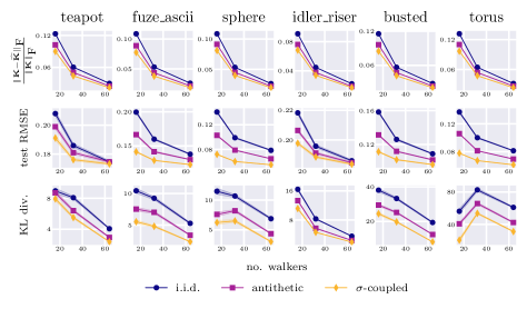
Figure 2: Graph-based GP regression results. $\sigma$-coupled GRFs give more accurate kernel estimates, better predictions and better uncertainty estimates. Estimates of standard deviations are shaded.

Probabilistic interpolation of traffic data. To further demonstrate, we train a scalable graph-based GP on a traffic flow dataset of the highways of San Jose, California, curated by Borovitskiy et al. (2021) using data from Chen et al. (2001) and OpenStreetMap. The graph has $1016$ nodes, with the traffic speed available at $325$. With this sparse, noisy dataset, $\sigma$-coupled GRFs again give more accurate predictions and better uncertainty estimates. Full results are reported in App. F.3.

5 Discussion and outlook

OT provides a powerful paradigm for variance reduction with random features. It offers proof techniques and numerical algorithms for finding novel RF couplings on continuous and discrete input domains. Whilst the presence of variance reduction is unambiguous, the downstream benefits it provides are less clear. With GRFs for scalable GPs, variance reduction permits much better approximate inference (Sec. 4.2). With RFFs and RLFs, this is not the case (App. B.2). This surprising finding suggests that, though popular, variance reduction is not always the right goal.

Right framing, wrong cost function. The reason for this counterintuitive behaviour is that, even if a coupling guarantees lower variance pointwise kernel estimates $\{k(\bm{x}_{i},\bm{x}_{j})\}_{i,j=1}^{N}$, functions like the predictive mean and KL-divergence are highly nonlinear in these estimates. For example, they may involve inverting a Gram matrix. It is hard to predict how the bias and variance of these downstream quantities will depend on the distribution of the pointwise estimates; they are not guaranteed to improve. Couplings that reduce the variance of $k(\bm{x}_{i},\bm{x}_{j})$ and $k(\bm{x}_{i},\bm{x}_{k})$ often also modify their covariance, which may effect downstream estimators that combine them. This includes seemingly innocuous quantities like the KL divergence from the true to the approximate prior (App. B.2).

We posit that OT provides the right framing for the problem of coupling RFs, but sometimes pointwise kernel variance is the wrong cost function. This naive choice may not fully capture how the joint distribution over kernel estimates determines downstream performance. Coupling to optimise e.g. the spectral properties of $\widehat{\mathbf{K}}$ may prove better (Choromanski et al., 2018; Avron et al., 2017a). Fortunately, OT provides a suite of theoretical and numerical tools achieve this; one simply modifies the cost function in Eq. 2. We hope this research will spur further work in this exciting direction.

6 Contributions and acknowledgements

Relative contributions. IR conceptualised the project, proposed the coupling mechanisms in Defs 3.3 and 4.1, proved the major theoretical contributions, ran the GRF experiments and wrote the manuscript. SM designed and ran the RFF and RLF GP experiments (Sec. 3.3), helped shape the project’s direction and made core contributions to the text. KC acted as the senior lead, providing technical guidance and developing the algorithms for the matching problem in App. C.3.1. RET met frequently throughout the project, giving important advice and support. AW provided helpful discussion, supervision and feedback on the manuscript.

Acknowledgements and funding. IR acknowledges support from a Trinity College External Studentship. SM acknowledges funding from the Vice Chancellor’s and the George and Marie Vergottis scholarship of the Cambridge Trust, and the Qualcomm Innovation Fellowship. RET is supported by Google, Amazon, ARM, Improbable and an EPSRC grant EP/T005386/1. AW acknowledges support from a Turing AI fellowship under grant EP/V025279/1 and the Leverhulme Trust via CFI.

We thank Bruno Mlodozeniec for his suggestion to use copulas in Sec. 3.2 and Mark Rowland for insightful discussions about multi-marginal optimal transport and the limitations of pointwise variance reduction. Viacheslav Borovitskiy helped guide our discussion of scalable graph-based GPs and, together with Iskander Azangulov, kindly provided updated code for loading the traffic data graph in Sec. 4.2 and App. F.3. We thank Matt Ashman and Arijit Sehanobish for their thoughtful feedback on the text, and Jihao Andreas Lin for interesting suggestions about possible GP applications.

Appendix A Solving the OT problem for RFFs and RLFs

In this appendix, we provide proofs for the theoretical results in Sec. 3.1 and supplement the discussion of copula-based numerical OT solvers in Sec. 3.2.

A.1 Proof of Lemma 3.1

We begin by proving Lemma 3.1, which formulates variance reduction for RFFs and RLFs as an optimal transport problem. We will first reason about the simpler case of RLFs, then consider RFFs.

Proof of Lemma 3.1. Consider the following recently-derived result by Reid et al. [2023].

Lemma A.1 (Kernel estimator MSE for RLFs [Reid et al., 2023]).

When estimating the Gaussian kernel $k(\bm{x},\bm{y})\coloneqq\exp(-\|\bm{x}-\bm{y}\|_{2}^{2}/2)$ for datapoints $\{\bm{x},\bm{y}\}\subset\mathbb{R}^{d}$ using random Laplace features (synonymously, positive random features), the mean square error of the kernel estimate $\widehat{k}(\bm{x},\bm{y})$ is given by:

$$\textrm{MSE}(\widehat{k})=\frac{e^{-2x^{2}-2y^{2}}}{m}\left((e^{2v^{2}}-e^{v^{2}})+(m-1)(\rho(\bm{x},\bm{y})-e^{v^{2}})\right)$$ (15)

where $m$ is the number of sampled random frequencies, $v\coloneqq\|\bm{x}_{i}+\bm{x}_{j}\|_{2}$ is a data-dependent scalar and $\rho(\bm{x}_{i},\bm{x}_{j})$ is the RF-conformity,

$$\rho(\bm{x},\bm{y})\coloneqq\frac{\Gamma(\frac{d}{2})}{m(m-1)}\sum_{i,j\neq i}\mathbb{E}_{\omega_{ij}}\left(\sum_{k=0}^{\infty}\frac{v^{2k}\omega_{ij}^{2k}}{2^{2k}k!\Gamma(k+\frac{d}{2})}\right).$$ (16)

Here, $\omega_{ij}\coloneqq\|\bm{\omega}_{i}+\bm{\omega}_{j}\|_{2}$ is the norm of the resultant of a pair of distinct frequencies and $\Gamma$ is the Gamma function.

Proof. Reid et al. [2023]. ∎

The simple derivation, reported in full by Reid et al. [2023], is based on rewriting the angular integral as a Hankel transform, yielding a Bessel function of the first kind with a known Taylor expansion.

Supposing that $\bm{\omega}_{i}\perp\bm{\omega}_{j}$, we have that $\omega_{ij}=\sqrt{\omega_{i}^{2}+\omega_{j}^{2}}$, where $\omega_{i}\coloneqq\|\bm{\omega}_{i}\|_{2}$ denotes the $L_{2}$-norm of the frequency $\bm{\omega}_{i}$. Note that, for $\bm{\omega}_{i}$ to be marginally Gaussian, we require that the marginal distribution over its norm is $\chi_{d}$, a Chi distribution with $d$ degrees of freedom. Substituting this into Eq. 15 and dropping terms unmodified by the coupling and irrelevant multiplicative factors, it is straightforward to arrive at the expression for the cost function $c_{\textrm{RLF}}$ in Eq. 7.

Finding the cost function for RFFs is only slightly more difficult. We begin by citing another recent result by Reid et al. [2023].

Lemma A.2 (Kernel estimator MSE for RFFs [Reid et al., 2023]).

When estimating the Gaussian kernel $k(\bm{x},\bm{y})\coloneqq\exp(-\|\bm{x}-\bm{y}\|_{2}^{2}/2)$ for datapoints $\{\bm{x},\bm{y}\}\subset\mathbb{R}^{d}$ using random Fourier features, the mean square error of the kernel estimate $\widehat{k}(\bm{x},\bm{y})$ is given by:

$$\text{MSE}(\widehat{k})=\frac{1}{m}\left(\frac{(1-e^{-z^{2}})^{2}}{2}+(m-1)(\zeta(\bm{x},\bm{y})-e^{-z^{2}})\right)$$ (17)

where $m$ is the number of samples, $\bm{z}\coloneqq\bm{x}-\bm{y}$ and $\zeta(\bm{x},\bm{y})$ is defined by

$$\zeta(\bm{x},\bm{y})\coloneqq\frac{1}{m(m-1)}\sum_{i,j\neq i}\mathbb{E}_{\bm{\omega}_{i},\bm{\omega}_{j}}\left[\cos(\bm{\omega}_{i}^{\top}\bm{z})\cos(\bm{\omega}_{j}^{\top}\bm{z})\right].$$ (18)

Proof. Reid et al. [2023]. ∎

Note the close resemblance to Eq. 16. The only term that depends on couplings between the random frequencies $\{\bm{\omega}_{i}\}_{i=1}^{m}$ is $\zeta(\bm{x},\bm{y})$, which we seek to suppress with carefully engineered correlations. From elementary trigonometry, $\cos\bm{\omega}_{i}^{\top}\bm{z}\cos\bm{\omega}_{j}^{\top}\bm{z}=\frac{1}{2}(\cos\left((\bm{\omega}_{i}+\bm{\omega}_{j})^{\top}\bm{z}\right)+\cos\left((\bm{\omega}_{i}-\bm{\omega}_{j})^{\top}\bm{z}\right)$, and for any coupling scheme $\bm{\omega}_{i}\pm\bm{\omega}_{j}$ is isotropic. Defining the random variables $\omega^{(+)}\coloneqq\|\bm{\omega}_{i}+\bm{\omega}_{j}\|_{2}$ and $\omega^{(-)}\coloneqq\|\bm{\omega}_{i}-\bm{\omega}_{j}\|_{2}$ and integrating out the angular part,

$$\zeta(\bm{x}_{i},\bm{x}_{j})=\frac{1}{m(m-1)}\sum_{i,j\neq i}\Gamma(d/2)2^{\frac{d}{2}-2}\mathbb{E}_{\omega^{(\pm)}}\left[(\omega^{(+)}z)^{1-\frac{d}{2}}J_{\frac{d}{2}-1}(\omega^{(+)}z)+(\omega^{(+)}z)^{1-\frac{d}{2}}J_{\frac{d}{2}-1}(\omega^{(-)}z)\right]$$ (19)

where $J_{\alpha}(x)$ is a Bessel function of the first kind, order $\alpha$. If $\bm{\omega}_{i}\perp\bm{\omega}_{j}$, $\omega^{(+)}=\omega^{(-)}$ so their distributions are identical. It follows that we can write

$$\zeta(\bm{x},\bm{y})=\frac{\Gamma(\frac{d}{2})}{m(m-1)}\sum_{i,j\neq i}\mathbb{E}_{\omega_{i},\omega_{j}}\left[\sum_{k=0}^{\infty}\frac{(-1)^{k}z^{2k}\left(\omega_{i}^{2}+\omega_{j}^{2}\right)^{k}}{2^{2k}k!\Gamma(k+\frac{d}{2})}\right].$$ (20)

Again dropping multiplicative factors and terms unmodified by the coupling, we arrive at the RFF OT cost function $c_{\textrm{RFF}}$ specified in Eq. 7. This completes the derivation. ∎

A.2 Proof of Thm. 3.2

We now solve the OT problem formulated in Lemma 3.1 exactly in the special case that $m=2$ (with mild asymptotic assumptions for RFFs). For the reader’s convenience, we copy it from the main text below.

Theorem A.3 (Solution to OT problem when $m=2$).

Denote by $F_{\chi_{d}}(\cdot)$ the cumulative distribution function of $\chi_{d}$. Considering $m=2$ orthogonal frequencies with norms $(\omega_{1},\omega_{2})$, the OT problem in Eq. 6 is solved by the negative monotone coupling

$$F_{\chi_{d}}(\omega_{1})+F_{\chi_{d}}(\omega_{2})=1$$ (21)

when $\frac{z^{2}}{d}\to 0$ for RFFs and in full generality for RLFs.

The proof of Thm. 3.2 uses ideas from optimal transport theory. In particular, it modifies arguments made for a related problem by (among others) Thorpe [2019], to which we direct the interested reader for further context and discussion. Before giving the proof, we establish some basic definitions and results.

Definition A.4 ($c$-monotone sets).

Given a cost function $c:\mathbb{R}^{d}\times\mathbb{R}^{d}\to\mathbb{R}$, we refer to a set $\Gamma\in\mathbb{R}^{2}$ as $c$-monotone if for all pairs $(x_{1},y_{1}),(x_{2},y_{2})\in\Gamma$ we have that

$$c(x_{1},y_{1})+c(x_{2},y_{2})\leq c(x_{1},y_{2})+c(x_{2},y_{1}).$$ (22)

It is intuitive that $c$-monotonicity should be a property of the support of Kantorovich optimal transport plan: if we could have accessed lower cost by sending $x_{1}\to y_{2}$ and $x_{2}\to y_{1}$ instead of $x_{1}\to y_{1}$ and $x_{2}\to y_{2}$, the plan would have done this instead. This is formalised as follows.

Lemma A.5 (Support of optimal transport plan is $c$-monotone [Thorpe, 2019]).

Consider $\eta\in\mathcal{P}(\mathbb{R})$, and assume that $\mu^{*}\in\Lambda(\eta)$ is the Kantorovich optimal transport plan for a continuous cost function $c(x,y)$. Then for all $(x_{1},y_{1}),(x_{2},y_{2})\in\emph{{supp}}(\mu^{*})$ we have that

$$c(x_{1},y_{1})+c(x_{2},y_{2})\leq c(x_{1},y_{2})+c(x_{2},y_{1}).$$ (23)

Proof. Thorpe [2019]. ∎

We are now ready to provide our proof of Thm. 3.2.

Proof of Thm. 3.2. Inspecting the cost functions in Eq. 7, it is clear that in the special case $m=2$ we have that

$$c_{\textrm{RFF}}(\omega_{1},\omega_{2})=\sum_{k=0}^{\infty}\frac{(-1)^{k}z^{2k}\left(\omega_{1}^{2}+\omega_{2}^{2}\right)^{k}}{2^{2k}k!\Gamma(k+\frac{d}{2})},\quad c_{\textrm{RLF}}(\omega_{1},\omega_{2})=\sum_{k=0}^{\infty}\frac{v^{2k}(\omega_{1}^{2}+\omega_{2}^{2})^{k}}{2^{2k}k!\Gamma(k+\frac{d}{2})},$$ (24)

with $z\coloneqq\|\bm{x}-\bm{y}\|_{2}$ and $v\coloneqq\|\bm{x}+\bm{y}\|_{2}$ as usual.

First consider $c_{\textrm{RLF}}$. We claim that for any $x_{1},x_{2},y_{1},y_{2}\geq 0$ satisfying Eq. 23 for this $c_{\textrm{RLF}}$, $x_{1}<x_{2}$ implies $y_{1}\geq y_{2}$. This is seen by observing that

$$\begin{multlined}c_{\textrm{RLF}}(x_{1},y_{1})+c_{\textrm{RLF}}(x_{2},y_{2})-c_{\textrm{RLF}}(x_{1},y_{2})-c_{\textrm{RLF}}(x_{2},y_{1})\\ =\sum_{k=0}^{\infty}\frac{v^{2k}}{2^{2k}k!\Gamma(k+\frac{d}{2})}\left[(x_{1}^{2}+y_{1}^{2})^{k}+(x_{2}^{2}+y_{2}^{2})^{k}-(x_{1}^{2}+y_{2}^{2})^{k}-(x_{2}^{2}+y_{1}^{2})^{k}\right]\\ =\sum_{k=0}^{\infty}\frac{v^{2k}}{2^{2k}k!\Gamma(k+\frac{d}{2})}\sum_{i=0}^{k}{k\choose i}\left[(y_{2}^{2})^{k-i}-(y_{1}^{2})^{k-i}\right]\left[(x_{2}^{2})^{i}-(x_{1}^{2})^{i}\right].\end{multlined}c_{\textrm{RLF}}(x_{1},y_{1})+c_{\textrm{RLF}}(x_{2},y_{2})-c_{\textrm{RLF}}(x_{1},y_{2})-c_{\textrm{RLF}}(x_{2},y_{1})\\ =\sum_{k=0}^{\infty}\frac{v^{2k}}{2^{2k}k!\Gamma(k+\frac{d}{2})}\left[(x_{1}^{2}+y_{1}^{2})^{k}+(x_{2}^{2}+y_{2}^{2})^{k}-(x_{1}^{2}+y_{2}^{2})^{k}-(x_{2}^{2}+y_{1}^{2})^{k}\right]\\ =\sum_{k=0}^{\infty}\frac{v^{2k}}{2^{2k}k!\Gamma(k+\frac{d}{2})}\sum_{i=0}^{k}{k\choose i}\left[(y_{2}^{2})^{k-i}-(y_{1}^{2})^{k-i}\right]\left[(x_{2}^{2})^{i}-(x_{1}^{2})^{i}\right].$$ (25)

Supposing that $x_{1}<x_{2}$, Eq. 23 is satisfied if and only if $y_{1}\geq y_{2}$, verifying the statement.

Denote by $\Gamma_{\textrm{RLF}}\coloneqq\textrm{supp}(\mu^{*})$ the support of the optimal transport plan for the cost function $c_{\textrm{RLF}}$, and consider some point $(x_{0},y_{0})\in\Gamma$. An immediate implication of the statement above is that

$$\Gamma_{\textrm{RLF}}\subset\{(x,y):x\leq x_{0},y\geq y_{0}\}\cup\{(x,y):x\geq x_{0},y\leq y_{0}\}.$$ (26)

Let $A=[0,x_{0}]\times[y_{0},\infty)$, $B=[0,x_{0})\times[0,y_{0})$, $C=[x_{0},\infty)\times[0,y_{0}]$ and $D=(x_{0},\infty]\times(y_{0},\infty]$. Note that $A\cup B\cup C\cup D=\mathbb{R}^{+}\times\mathbb{R}^{+}$ so $\mu^{*}(A\cup B\cup C\cup D)=1$ since the measure is normalised. The subsets are also disjoint apart from $A\cap C=(x_{0},y_{0})$, a singleton of zero measure. Eq. 26 implies that $\mu^{*}(B)=0=\mu^{*}(D)$, whereupon $1=\mu^{*}(A\cup C)=\mu^{*}(A)+\mu^{*}(C)=\mu^{*}(A\cup B)+\mu^{*}(C\cup B)$. Now $A\cup B=([0,x_{0}]\times\mathbb{R}^{+})\backslash(\{x_{0}\}\times[0,y_{0}))$ and the set $\{x_{0}\}\times[0,y_{0})$ is zero measure. Therefore, $\mu^{*}(A\cup B)=\mu^{*}([0,x_{0}]\times\mathbb{R}^{+})=F_{\chi_{d}}(x_{0})$. Likewise, $\mu^{*}(C\cup B)=\mu^{*}(\mathbb{R}^{+}\times[0,y_{0}])=F_{\chi_{d}}(y_{0})$. Relabelling $(x_{0},y_{0})\in\Gamma$ by $(\omega_{1},\omega_{2})$, Eq. 21 immediately follows. This completes the proof that negative monotone coupling minimises the kernel estimator variance for orthogonal RLFs.

Let us now turn to the case of RFFs. The optimal transport plan $\mu^{*}$ will instead be $c_{\textrm{RFF}}$-monotone. Unfortunately, Eq. 25 does not hold in general for $c_{\textrm{RFF}}$, so we cannot immediately use the same arguments to conclude that the OT plan is negative monotone. However, Eq. 25 does hold if we just consider the first nontrivial term in the Taylor expansion in $z$ or $\frac{1}{d}$. In particular, dropping terms that are not modified by a coupling (i.e. depend only on $\omega_{1}$ or $\omega_{2}$),

$$c_{\textrm{RFF}}(\omega_{1},\omega_{2})=\frac{z^{4}}{\Gamma(\frac{d}{2}+2)}\left[\frac{\omega_{1}^{2}\omega_{2}^{2}}{16}+\mathcal{O}\left(\frac{z^{2}}{d}\right)\right].$$ (27)

It is straightforward to show that, if we take the $\frac{z^{2}}{d}\to 0$ limit so we can neglect higher-order terms, $c_{\textrm{RFF}}$ indeed satisfies Eq. 25 and we can make the same arguments about $\Gamma_{\textrm{RFF}}$ as with $\Gamma_{\textrm{RLF}}$. In this limit, the optimal transport plan is again negative monotone. The proof is then complete. ∎

Comments on the $z^{2}/d\to 0$ limit for RFFs. We have seen that for RFFs it is only possible to solve the OT problem in Eq. 6 exactly in the $z^{2}/d\to 0$ asymptotic limit. Here, we comment on why this result is nonetheless interesting and useful. Firstly, note that in practice pairwise norm coupling still substantially suppresses kernel estimator variance, even at data lengthscales chosen by training an exact GP independent of the RF construction (Table 1). Even if at bigger $z$ the method no longer provides the smallest possible estimator variance, it can still substantially reduce it compared to an i.i.d. coupling. Second, from a more theoretical perspective, the $d\to\infty$, small sample regime is exactly where standard QMC methods often fail. It is interesting that OT-driven methods can still provide theoretical guarantees in this low-sample, high-dimensionality setting. Last, we note that, for RFF variance reduction schemes, it is very common to only guarantee gains in the asymptotic limit. This is also the case e.g. for orthogonality [Reid et al., 2023, Yu et al., 2016]: a well-established and widely-used algorithm.

A.3 Proof of Corollary 3.4

We now prove that pairwise norm-coupled RFs (Def. 3.3) provide strictly lower kernel estimator variance than i.i.d. RFs.

Proof of Corollary 3.4. Supposing that we have $m=d$ frequencies, the sum $\sum_{i,j\neq i}^{d}$ has $d(d-1)$ terms in total. Of these, $2\lfloor\frac{d}{2}\rfloor$ correspond are negative monotone norm couplings, and the remainder are independent. The independent terms are the same in the pairwise norm-coupled and fully i.i.d. configurations, so can be ignored. By Thm. 3.2, we have seen that negative monotone coupling exactly solves the variance reduction OT problem (under mild asymptotic assumptions for RFFs), so these variance contributions will be strictly smaller in the norm-coupled case. It immediately follows that pairwise norm-coupled RFs give strictly lower kernel estimator variance than orthogonal independent-norm RFs, so the result follows. ∎

A.4 Proof of Thm. 3.5

We now drop the restriction that $\widehat{\bm{\omega}}_{1}\perp\widehat{\bm{\omega}}_{2}$ and consider the variance reduction problem for $m=2$ frequencies whose respective direction is unconstrained. We will prove Thm. 3.5, which asserts that in this case the best possible coupling is antithetic, $\bm{\omega}_{1}=-\bm{\omega}_{2}$.

Proof of Thm. 3.5. Recalling the expression for RLF variance in Lemma A.1, the more general OT problem under consideration is

$$\mu^{*}=\arg\inf_{\mu\in\Lambda_{2}(\mathcal{N})}\left[\mathbb{E}_{\bm{\omega}_{1},\bm{\omega}_{2}\sim\mu}\sum_{k=0}^{\infty}\frac{v^{2k}\|\bm{\omega}_{1}+\bm{\omega}_{2}\|_{2}^{k}}{2^{2k}k!\Gamma(k+\frac{d}{2})}\right].$$ (28)

The term in square parentheses is an expectation of an infinite sum, every term of which is greater than or equal to $0$. The sum is manifestly minimised if $\|\bm{\omega}_{1}+\bm{\omega}_{2}\|_{2}=0$, which sets every term (apart from the first) to $0$. This is achieved if and only if $\bm{\omega}_{1}=-\bm{\omega}_{2}$: a valid coupling called ‘antithetic sampling’. Any other joint distribution assigns nonzero probability to the event $\|\bm{\omega}_{1}+\bm{\omega}_{2}\|_{2}>0$, so this optimal coupling is unique. ∎

A.5 Copulas as numerical OT solvers

copula_schematic

Figure 3: Schematic of a $2$-dimensional Gaussian copula. Random variables drawn from a Gaussian distribution with unit diagonal covariances (i.e. a correlation matrix) will be marginally normally distributed, $\mathcal{N}(0,1)$. Correlations between the variables will be controlled by the off-diagonal covariances. We can push each coordinate forward using the Gaussian CDF $F_{\mathcal{N}}$ to get marginally uniform random variables, then again with $F_{\chi_{d}}^{-1}$ to get marginal Chi distributions. In Sec. 3.2 and App. A.5, we describe techniques to learn the optimal covariance matrix by gradient descent, directly minimising the kernel approximation error. In doing so, we find a numerical approximation of the solution to the multi-marginal OT problem in Eq. 6.

In the main text, we noted that finding an analytic solution to the multi-marginal OT problem for RFFs and RLFs (Eq. 6) is an open problem. In Sec. 3.2, we briefly presented an alternative numerical approach using copulas. Here, we discuss this in greater detail. Fig. 3 gives a visual overview.

Copulas. A copula is a multivariate cumulative distribution function (CDF) whose marginals are uniformly distributed on $[0,1]$. By Sklar’s theorem [Sklar, 1959], its joint distribution can be arbitrary. Given a copula, we can easily enforce the constraint that its marginals are $\chi_{d}$ by pushing each coordinate forward with the inverse CDF $F_{\chi_{d}}^{-1}(\cdot)$, whilst retaining necessary flexibility in the joint to reduce estimator variance. Copulas can be used to model dependencies between random variables and are popular tools in quantitative finance [Haugh, 2016].

Gaussian copulas. The general family of copulas is still intractable to optimise and sample from so we constrain ourselves to Gaussian copulas. These are distributions with uniform marginals whose joint distributions are determined by multivariate Gaussians, defined below.

Definition A.6 (Gaussian copula).

Let $\{\omega_{i}\}_{i=1}^{m}\sim\mathcal{N}(0,\bm{\Sigma})$ where $\bm{\Sigma}\in\mathbb{R}^{m\times m}$ is a correlation matrix, i.e. a positive definite matrix with unit diagonals, and let $F_{\mathcal{N}}$ be the CDF of the standard univariate Gaussian. We say $\{F_{\mathcal{N}}(\omega_{i})\}_{i=1}^{m}$ is distributed according to a Gaussian copula with covariance $\bm{\Sigma},$ and use the notation $\{F_{\mathcal{N}}(\omega_{i})\}_{i=1}^{m}\sim\text{GC}(\bm{\Sigma})$ to denote this.

Parameterising correlation matrices. Gaussian copulas are easy to sample from since they involve sampling a multivariate Gaussian and applying the univariate Gaussian CDF. We are therefore left with the task of finding an appropriate correlation matrix $\bm{\Sigma},$ for which we turn to numerical optimisation. The family of $m\times m$ correlation matrices can be parameterised by a vector $\bm{\theta}\in\mathbb{R}^{m(m-1)/2}.$ In fact, there exist tractable bijections between unconstrained vectors of real numbers $\bm{\theta}\in\mathbb{R}^{m(m-1)/2}$ and lower triangular Cholesky factors $\mathbf{L}_{\bm{\theta}}$ such that $\bm{\Sigma}=\mathbf{L}_{\bm{\theta}}\mathbf{L}_{\bm{\theta}}^{\top}$ is a valid correlation matrix [Bhat and Mondal, 2021]. In particular, suppose that for each $i=1,\dots,N,$ and $j=1,\dots,i,$ we have $\theta_{ij}\in\mathbb{R}^{+},$ where $\theta_{ii}=1.$ Then the parameterisation we use is

$$L_{ij}=\begin{cases}\frac{\theta_{ij}}{s_{i}}&\text{ for }i\leq j,\\ 0&\text{ otherwise},\end{cases}$$ (29)

where $s_{i}=\sqrt{\sum_{j=1}^{i}{\theta_{ij}^{2}}}.$ Note that, since we are directly parameterising the Cholesky factor, we can sample from the associated Gaussian copula with an $\mathcal{O}(m^{2})$ computational cost.

Optimising correlation matrices. In order to pick an appropriate correlation matrix $\bm{\Sigma},$ we optimise it directly to minimise the root mean squared error (RMSE) loss

$$\mathcal{L}(\bm{\theta})=\mathbb{E}_{\omega_{i}}\left[\sqrt{\frac{1}{N^{2}}\sum_{i,j=1}^{N}(\phi_{\text{RF}}(\bm{x}_{i})^{\top}\phi_{\text{RF}}(\bm{x}_{j})-k(\bm{x}_{i},\bm{x}_{j}))^{2}}~{}\right],$$ (30)

where $\omega_{i}\sim\text{GC}(\mathbf{L}_{\bm{\theta}}\mathbf{L}_{\bm{\theta}}^{\top}).$ Note that $\phi_{\text{RF}}$ here depends on $\omega_{i},$ though we have suppressed this dependence for notational simplicity. Assuming that $\phi_{\text{RF}}$ is differentiable with respect to $\omega_{i},$ which is the case in RFFs and RLFs, we can optimise the copula parameters $\bm{\theta}$ by estimating the loss in Eq. 30, computing its gradients with respect to $\bm{\theta},$ and updating its values accordingly.

Training curves. Fig. 4 shows an example of training curves for RFFs and RLFs using a numerically optimised Gaussian copula to learn an appropriate norm-coupling, here on the Boston dataset. We observe that the numerically optimised copula recovers the performance of the pairwise norm coupling scheme we proposed. This suggests that the proposed scheme may in fact be (close to) optimal. Rigorous analytical investigation is an important avenue for future work.

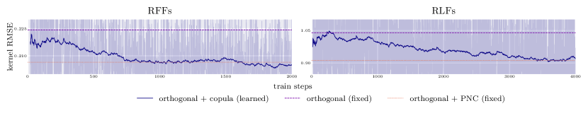
Figure 4: Training RMSE losses on a split of the Boston dataset. For the ‘orthogonal + copula (learned)’ configuration, we display the raw training loss (light blue) as well as an exponential moving average (dark blue). The performance of the coupling scheme returned by optimising the copula matches the performance of the ‘orthogonal + PNC’ scheme that we proved is optimal for the $m=2$ case. The optimisation is very noisy but this can be mitigated by increasing the number of samples used in the reparameterisation trick.

Appendix B RFF and RLF experimental details

In this appendix, we supplement the discussion in Sec. 3.3, providing more details of our experimental setup for Gram matrix estimation. We also apply norm-coupled RFs to sparse spectrum Gaussian processes [Lázaro-Gredilla et al., 2010], explaining the surprising closing remarks of Sec. 3 that in this case variance reduction does not help downstream performance.

B.1 Details for RFF and RLF experiments

Overview. In both our RFF and RLF experiments, we compare different coupling schemes for approximating the Gaussian kernel. The Gaussian kernel, including a lengthscale parameter $\ell,$ an output scale variable $\sigma_{v}$ and a noise scale parameter $\sigma_{n}$, takes the form

$$k(x_{i},x_{j})=\sigma_{v}^{2}\exp\left(-\frac{1}{2\ell^{2}}||\bm{x}_{i}-\bm{x}_{j}||_{2}^{2}\right).$$

Our baselines include standard methods for sampling random frequency vectors for use within RFFs and RLFs: i.i.d. sampling and Halton sequences [Halton, 1960]. In addition, for both settings, we consider ensembles of frequency vectors that are coupled to have orthogonal directions but i.i.d. lengths. For a dataset of dimension $d,$ for RFFs we use ensembles of $d$ orthogonal vectors. For RLFs we use ensembles of $2d$ vectors, including $d$ orthogonal basis vectors and their $d$ antiparallel vectors.

Selecting kernel hyperparameters. We want to compare our coupling schemes using realistic kernel hyperparameter values, which we determine as follows. A realistic application setting for RFFs is within GPs for probabilistic regression. Therefore, we first fit a GP on a tractable subset of the data, specifically a maximum of 256 randomly chosen datapoints, to select appropriate parameters $\ell,\sigma_{v}$ and $\sigma_{n}.$ We optimise the exact GP marginal likelihood with respect to these hyperparameters, and subsequently fix them. On the other hand, it is well-documented that RLFs suffer from poor estimator concentration when the data norm becomes large because of the exponential function in the feature map (Eq. 5); see e.g. Thm. 4 and App. F6 of Choromanski et al. [2020] or Thm. 4.3 of Likhosherstov et al. [2022], where the authors bound the $L_{2}$-norm of queries and keys. This is anecdotally responsible for the deterioration in performance of Performers when networks become very deep. To reflect this fact and choose a data regime where vanilla RLFs can perform reasonably well (so we can assess any gains from our coupling), we set the lengthscale $\ell$ to two twice the average summed norm of the data, namely

$$\ell=\frac{2}{N_{\textrm{train}}^{2}}\sum_{i,j=1}^{N_{\textrm{train}}}||\bm{x}_{i}+\bm{x}_{j}||_{2},$$ (31)

over the training set. We train the rest of the kernel parameters ($\sigma_{v}$ and $\sigma_{n}$) to maximise the marginal likelihood of the data under the exact GP.

Splitting procedure. To obtain mean evaluation metrics and standard errors, we evaluate the methods on multiple random splits as follows. For each dataset, we conduct cross validation with 20 splits, splitting each dataset into a training and a test set. Because we train an exact GP to determine kernel hyperparameters and evaluate its predictive NLL, we need to limit the number of datapoints used in both the training and the test set. We set them to a maximum of 256 points each by sub-sampling at random without replacement. After training the GP, we evaluate the metrics on the test set, and repeat this procedure for all 20 splits.

Optimisation details. We train the exact GP using the Adam optimiser [Kingma and Ba, 2014], using a learning rate of $10^{-2}.$ The exact GP optimisation stage converges around $1000$ steps, and we run it up to $5000$ steps.

B.2 Do better kernel approximations give better predictions?

Kernel and posterior approximations. Suppose that we have drawn an ensemble of frequency vectors from which we construct random features $\{\phi_{\text{RF}}(\bm{x}_{i})_{i=1}^{N}\}$. Group these in a large design matrix $\bm{\Phi}$,

$$\bm{\Phi}\coloneqq[\phi_{\text{RF}}(\bm{x}_{i})]_{i=1}^{N},$$ (32)

where $\phi_{\text{RF}}(\bm{x}_{i})$ of course depends on the ensemble frequencies $\{\bm{\omega}_{i}\}_{i=1}^{m}$ (suppressed for notational compactness). For RFFs $\bm{\Phi}\in\mathbb{R}^{N\times 2m}$ whereas for RLFs $\bm{\Phi}\in\mathbb{R}^{N\times m}$. We estimate the Gram matrix by $\widehat{\mathbf{K}}\coloneqq\bm{\Phi}\bm{\Phi}^{\top}$.

As noted by Lázaro-Gredilla et al. [2010], this RF kernel approximation is exactly equivalent to a linear model, namely

$$\bm{y}=\bm{w}\bm{\Phi}+\bm{\epsilon},$$ (33)

where $\bm{w}\sim\mathcal{N}(\bm{0},\mathbf{I})$ and $\bm{\epsilon}\sim\mathcal{N}(\bm{0},\sigma_{n}^{2}\mathbf{I}).$ The prior covariance of this linear model is $\bm{\Phi}^{\top}\bm{\Phi}+\sigma_{n}^{2}\mathbf{I},$ which is, by construction, equal in expectation to the exact covariance produced by the kernel, namely $\mathbf{K}+\sigma_{n}^{2}\mathbf{I}$. The predictive means of the approximate linear model and corresponding exact model are

$$\bm{\mu}_{\text{approx}} =\bm{\Phi}_{p}\left(\frac{1}{\sigma_{n}^{2}}\bm{\Phi}_{d}\bm{\Phi}_{d}^{\top}+\bm{I}\right)^{-1}\bm{\Phi}_{d}\bm{y},$$ (34)

$$\bm{\mu}_{\text{exact}} =\mathbf{K}_{pd}(\mathbf{K}_{dd}+\sigma_{n}^{2}\mathbf{I})^{-1}\bm{y},$$ (35)

whereas the predictive covariances are

$$\mathbf{C}_{\text{approx}} =\bm{\Phi}_{p}^{\top}\left(\frac{1}{\sigma_{n}^{2}}\bm{\Phi}_{d}\bm{\Phi}_{d}^{\top}+\bm{I}\right)^{-1}\bm{\Phi}_{p}+\sigma_{n}^{2}\mathbf{I},$$ (36)

$$\mathbf{C}_{\text{exact}} =\mathbf{K}_{pp}-\mathbf{K}_{pd}(\mathbf{K}_{dd}+\sigma_{n}^{2}\mathbf{I})^{-1}\mathbf{K}_{dp}.$$ (37)

Here, $\bm{\Phi}_{d}$ and $\bm{\Phi}_{p}$ are the design matrices corresponding to the training inputs and prediction outputs respectively, $\mathbf{K}_{dd}$ is the covariance matrix corresponding the training inputs, $\mathbf{K}_{pp}$ is the covariance matrix corresponding to the prediction inputs and $\mathbf{K}_{pd}$ and $\mathbf{K}_{dp}$ are the cross-covariance matrices between the training and prediction datapoints. These models become exactly equivalent in the limit of an infinite number of features $m$ since the kernel approximation becomes exact.

We have seen that pairwise norm coupling improves the approximation of the Gram matrices $\mathbf{K}$. In particular, we are able to suppress the variance of each pointwise kernel estimate (Thm. 3.2 and Corr. 3.4), and therefore the relative Frobenius norm error between the true and approximate Gram matrices (Table 1). In light of the discussion above, it would be natural to assume that this would result in more accurate approximations of the predictive mean and covariance. However, in the following section we will see that surprisingly this is not the case.

Evaluating posterior approximation quality. Table 2 takes the RFs from Sec. 3.3, where we found that our coupling can substantially improve the quality of kernel estimation. It then reports the KL divergence between the exact predictive posterior and the approximate predictive posteriors computed with RFFs and RLFs, respectively. To be clear, Eqs 34 and 36 can be rewritten

$$\bm{\mu}_{\text{approx}}=\widehat{\mathbf{K}}_{pd}(\widehat{\mathbf{K}}_{dd}+\sigma_{n}^{2}\bm{I})^{-1}\bm{y},~{}~{}~{}\mathbf{C}_{\text{approx}}=\widehat{\mathbf{K}}_{pp}-\widehat{\mathbf{K}}_{pd}(\widehat{\mathbf{K}}_{dd}+\sigma_{n}^{2}\mathbf{I})^{-1}\widehat{\mathbf{K}}_{dp}$$ (38)

where $\widehat{\mathbf{K}}_{dd}={\mathbf{\Phi}}_{d}^{\top}{\mathbf{\Phi}}_{d}$, $\widehat{\mathbf{K}}_{pd}={\mathbf{\Phi}}_{d}^{\top}{\mathbf{\Phi}}_{p}$, $\widehat{\mathbf{K}}_{pd}={\mathbf{\Phi}}_{p}^{\top}{\mathbf{\Phi}}_{d}$ and $\widehat{\mathbf{K}}_{pp}={\bm{\Phi}}_{p}^{\top}{\bm{\Phi}}_{p}.$ It is then straightforward to compute the KL divergence between Gaussian distributions with means $\bm{\mu}_{\text{approx}}$, $\bm{\mu}_{\text{exact}}$ and covariances $\mathbf{C}_{\text{approx}}$, $\mathbf{C}_{\text{exact}}$.

Fourier Features	Concrete	Abalone	CPU	Power	Airfoil	Boston
i.i.d.	$1.491$ $\pm 0.106$	$0.013$ $\pm 0.001$	$1.570$ $\pm 0.417$	$0.150$ $\pm 0.007$	$0.357$ $\pm 0.025$	$2.128$ $\pm 0.197$
Halton	$1.548$ $\pm 0.104$	$0.014$ $\pm 0.001$	$1.596$ $\pm 0.419$	$0.138$ $\pm 0.006$	$0.356$ $\pm 0.024$	$2.263$ $\pm 0.204$
Orthogonal	$1.166$ $\pm 0.113$	$0.004$ $\pm 0.000$	$1.635$ $\pm 0.423$	$0.029$ $\pm 0.002$	$0.235$ $\pm 0.017$	$1.990$ $\pm 0.191$
+ PNC	$1.168$ $\pm 0.113$	$0.004$ $\pm 0.000$	$1.589$ $\pm 0.416$	$0.029$ $\pm 0.002$	$0.235$ $\pm 0.017$	$1.985$ $\pm 0.190$
Laplace Features	Concrete	Abalone	CPU	Power	Airfoil	Boston
i.i.d.	$0.552$ $\pm 0.064$	$0.028$ $\pm 0.003$	$5.925$ $\pm 1.961$	$0.199$ $\pm 0.011$	$0.230$ $\pm 0.024$	$0.759$ $\pm 0.068$
Halton	$0.574$ $\pm 0.064$	$0.024$ $\pm 0.003$	$5.811$ $\pm 1.897$	$0.146$ $\pm 0.009$	$0.213$ $\pm 0.022$	$0.834$ $\pm 0.074$
Orthogonal	$0.486$ $\pm 0.059$	$0.014$ $\pm 0.002$	$5.494$ $\pm 1.774$	$0.059$ $\pm 0.005$	$0.165$ $\pm 0.018$	$0.679$ $\pm 0.058$
+ PNC + antithetic	$0.482$ $\pm 0.058$	$0.014$ $\pm 0.002$	$5.468$ $\pm 1.780$	$0.050$ $\pm 0.006$	$0.165$ $\pm 0.018$	$0.673$ $\pm 0.058$

Table 2: KL divergences (nats per datapoint) between exact and approximate GP predictive posterior on held out test sets. Note that we use $d$ features for RFFs and $2d$ features for RLFs. Reported errors are equal to two standard errors, i.e. $98\%$ confidence intervals, computed by averaging across splits. Note that differences between data splits are responsible the big errors; within each split we take enough trials that the standard errors become small. For every individual data split, orthogonal is statistically significantly better than i.i.d. but there is no additional benefit from PW norm-coupled. Results differ between splits because we consider a different subset of the dataset.

Surprisingly, we find that, even though our couplings improve the accuracy of kernel approximation, the approximate mean and covariance and hence the KL divergence to the true posterior do not necessarily improve. In Table 1 we routinely see variance reductions of $10$-$20$%, but even with very many trials this is not reflected in the data splits used for Table 2.

The reason for this experimental finding is that, as is clear in Eq. 38, the posterior is highly nonlinear in $\widehat{\mathbf{K}}$. This is on account of the presence of matrix multiplications and inversions. These nonlinear operations on the Gram matrix entries mean that, despite our pointwise estimates being unbiased, $\bm{\mu}_{\text{approx}}$ and $\mathbf{C}_{\text{approx}}$ are in fact biased. We have achieved our objective of variance reduction of $\widehat{\mathbf{K}}$ – with pairwise norm coupling, it is both theoretically mandated and empirically observed. But clearly this does not necessitate variance (or bias) reduction for $\bm{\mu}_{\text{approx}}$ and $\mathbf{C}_{\text{approx}}$. The relationship between the distribution of $\widehat{\mathbf{K}}$ and the distribution of the approximate posterior is more complex.

Variance reduction does not always help predictive performance. To sharpen this point, we now take a single data split of the power dataset and plot the the kernel approximation RMSE (i.e. kernel estimator variance), as well as various quantities of predictive interest, against the number of features $m$. We exclude the Halton coupling (which is consistently worse than ‘orthogonal’) for clarity of presentation. Fig. 5 shows the results.

The left hand panel confirms that we have achieved our stated objective of variance reduction. Moreover, for all couplings the quality of approximation improves as we introduce more ensembles of size $d$. Reading left to right, the other three panels show: (i) the KL divergence between the exact and approximate GP predictive posteriors (as in Table 2), (ii) the predictive RMSE on a held out test set, and (iii) the KL divergence between the exact and approximate GP priors. In every instance, orthogonality provides a substantial gain but, despite the encouraging results for kernel RMSE, there is no additional benefit from PNC. However, it would be wrong to draw the simplistic conclusion that PNC does not give large enough variance savings to see downstream gains: comparable reductions from orthogonality yield substantial improvements. The problem is more fundamental, relating to how the joint distribution of kernel estimates – beyond just the second moment of its pointwise entries – interacts with nonlinear operations like matrix multiplication and inversion.

A non-exhaustive list of publications with a substantial focus on reducing the variance of RF kernel estimates is given by: Yu et al. [2016], Rowland et al. [2018], Reid et al. [2023], Likhosherstov et al. [2022], Yang et al. [2014a], Le et al. [2013], Bojarski et al. [2017], Choromanski et al. [2017], Lyu [2017], Shen et al. [2017], Dao et al. [2017], Munkhoeva et al. [2018]. This can sometimes be a very effective approach for improving downstream performance; e.g. observe the benefits from $\sigma$-coupled GRFs in Sec. 4. But our findings suggest that the true reasons for any boost in performance are more complex than variance reduction alone. There has been some recognition that other properties of the kernel approximation are important e.g. for kernel ridge regression – in particular, the spectral properties of $\widehat{\mathbf{K}}$ [Choromanski et al., 2018, Avron et al., 2017a] – but we believe this to be underappreciated in the literature. More work is needed to fully identify the right desiderata for RF couplings in machine learning, and more algorithms to optimise couplings to improve them. OT provides an excellent framework for achieving this.

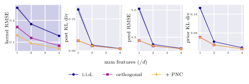
Figure 5: Results on a single train-test split of the power dataset, showing kernel approximation RMSE, KL divergence to the true predictive posterior, test RMSE of predictions and KL divergence to the true prior. We have successfully reduced the variance of the kernel approximation, but this may not help downstream metrics. Standard deviation estimates are shaded but too small to easily see.

Appendix C Graph random features

In this appendix, we provide a self-contained introduction to graph random features (GRFs) and previously-proposed techniques to reduce their variance. We also explain the motivations behind the series of approximations used in Sec. 4.1, and where possible provide empirical evidence that these approximations for tractability and efficiency do not substantially degrade the performance of the learned $\sigma$-coupling.

C.1 Constructing graph random features

For the reader’s convenience, we begin by providing a brief self-contained introduction to GRFs.

Graph node kernels. Recall that graph node kernels $k:\mathcal{N}\times\mathcal{N}\to\mathbb{R}$ are positive definite, symmetric functions defined on pairs of nodes of $\mathcal{G}$. Note that one can also define kernels that take pairs of graphs as inputs, but these are not the object of our study.

Many of the most popular graph node kernels in the literature are functions of weighted adjacency matrices [Smola and Kondor, 2003b, Chapelle et al., 2002]. In particular, they are often functions of the graph Laplacian matrix,

$$\mathbf{L}\coloneqq\mathbf{D}-\mathbf{W},$$ (39)

where $\mathbf{W}$ is a (weighted) adjacency matrix and $\mathbf{D}$ is a diagonal degree matrix (satisfying $\mathbf{D}_{ii}=\sum_{j}\mathbf{W}_{ij}$). It is also common to consider its normalised variant,

$$\widetilde{\mathbf{L}}\coloneqq\mathbf{D}^{-\frac{1}{2}}\mathbf{L}\mathbf{D}^{-\frac{1}{2}},$$ (40)

whose spectrum is contained in $[0,2]$ [Chung, 1997]. We provide examples in Table 3.

Name	Form
$d$-regularised Laplacian	$(\mathbf{I}_{N}+\sigma^{2}\mathbf{L})^{-d}$
$p$-step random walk	$(\alpha\mathbf{I}_{N}-\mathbf{L})^{p},\alpha\geq 2$
Diffusion	$\exp(-\sigma^{2}\mathbf{L}/2)$
Inverse Cosine	$\cos\left(\mathbf{L}\pi/4\right)$

Table 3: Examples of graph node kernels. The $\mathrm{exp}$ and $\mathrm{cos}$ mappings are defined via Taylor series expansions rather than element-wise, e.g. $\exp(\mathbf{M})\coloneqq\lim_{n\to\infty}(\mathbf{I}_{N}+\mathbf{M}/n)^{n}$ and $\cos(\mathbf{M})\coloneqq\textrm{Re}(\exp(i\mathbf{M}))$. $\sigma$ and $\alpha$ are regularisers.

Formula for graph random features. Computing graph node kernels exactly is computationally expensive because of the $\mathcal{O}(N^{3})$ cost of e.g. matrix inversion or exponentiation. Inspired by the success of random Fourier features in the Euclidean domain [Rahimi and Recht, 2007], the recently-introduced class of graph random features (GRFs) permits unbiased approximation of $k$ in subquadratic time [Choromanski, 2023, Reid et al., 2024b]. Intuitively, GRFs interpret the powers of weighted adjacency matrices in the Taylor expansions of the expressions in Table 3 as weighted sums over walks on a graph. Instead of computing this infinite sum of walks exactly, we can sample $m$ finite walks (using importance sampling) to construct an unbiased estimate of $k$.

Concretely, GRFs compute a set of estimators $\{\phi_{\textrm{GRF}}(v_{i})\}_{i\in\mathcal{N}}$ such that $k(v_{i},v_{j})=\mathbb{E}[\phi_{\textrm{GRF}}(v_{i})^{\top}\phi_{\textrm{GRF}}(v_{j})]$ by taking:

$$\phi_{\textrm{GRF}}(v_{i})=\frac{1}{m}\sum_{k=1}^{m}\psi(\bm{\omega}_{k}^{(i)}),$$ (41)

where $\bm{\omega}_{k}^{(i)}$ is the $k$th walk (out of a total of $m$) simulated out of the starting node $v_{i}$. We remind the reader that by a ‘walk’ we mean a sequence of neighbouring graph nodes. The projection function $\psi(\cdot):\Omega\to\mathbb{R}^{N}$ maps from then set of graph random walks $\Omega\coloneqq\left\{(v_{i})_{i=1}^{l}\,|\,v_{i}\in\mathcal{N},(v_{i},v_{i+1})\in\mathcal{E},l\in\mathbb{N}\right\}$ to a sparse $N$-dimensional feature vector. It is computed as follows:

$$\psi(\bm{\omega}^{(i)})_{q}\coloneqq\sum_{\omega_{iq}\in\Omega_{iq}}\frac{\widetilde{\omega}(\omega_{iq})f(\textrm{len}(\omega_{iq}))}{p(\omega_{iq})}\mathbb{I}(\omega_{iq}\in\bm{\omega}^{(i)}),\quad q=1,...,N.$$ (42)

In this expression,

• $\psi(\bm{\omega}^{(i)})_{q}$ is the $q$th component of the feature projection of the random walk $\bm{\omega}^{(i)}$ (itself a sequence of neighbouring graph nodes beginning with $v_{i}$).

• $\Omega_{iq}$ is the set of all graph walks between nodes $v_{i}$ and $v_{q}$, of which each $\omega_{iq}$ is a member.

• $\mathbb{I}(\cdot)$ is the indicator function that evaluates to $1$ if its argument is true and $0$ otherwise.

• $\omega_{iq}\in\bm{\omega}^{(i)}$ is the condition that $\omega_{iq}$, a particular walk between nodes $v_{i}$ and $v_{q}$, is a prefix subwalk of $\bm{\omega}^{(i)}$, the random walk we actually sample.

• $f:\mathbb{N}\to\mathbb{R}$ is the modulation function, which controls the particular graph node kernel we choose to approximate.

• $\textrm{len}(\omega_{iq})$ is the length of graph walk $\omega_{iq}$.

• $p(\omega_{iq})$ is the marginal probability of sampling a random walk $\omega_{iq}$, which is known from the sampling strategy.

• $\widetilde{\omega}(\omega_{iq})$ is a function that returns the products of weights of the edges traversed by $\omega_{iq}$.

Intuitively, to construct $\psi(\bm{\omega}^{(i)})$ using a random walk $\bm{\omega}^{(i)}$, we look at the node that it visits at each of the $\textrm{len}(\bm{\omega}^{(i)})+1$ timesteps before termination. At every node, we add a contribution to the feature at the corresponding coordinate that depends on (i) the product of edge weights traversed so far, (ii) the known marginal probability of sampling the walk so far, and (iii) a ‘modulation function’ $f$ applied to the number of steps taken so far. We refer the reader to the original works of Choromanski [2023] and Reid et al. [2024b] for further technical details, experimental results and a proof of unbiasedness.

C.2 Antithetic termination

In this section, we briefly describe antithetic termination [Reid et al., 2024c]: a previously-proposed variance reduction algorithm that couples the lengths of pairs of random walks.

Consider a random walker that terminates with probability $p$ at every timestep. In practice, this can be achieved by drawing a ‘termination random variable’ $t$ from a uniform distribution on $[0,1]$, $t\sim\mathcal{U}([0,1])$, and ending the walk if $t<p$. Now consider two such walkers with corresponding termination random variables $t_{1},t_{2}$. If they are independent, $t_{1}$ and $t_{2}$ are drawn independently. Antithetic termination instead proposes to induce a nontrivial joint distribution by first drawing $t_{1}\sim\mathcal{U}([0,1])$ as usual, and then setting $t_{2}=\mod_{1}(t_{1}+\frac{1}{2})$. $t_{2}$ still follows a uniform marginal distribution so we preserve unbiasedness, but this coupling forces walkers to terminate at different timesteps (if $p<0.5$) which the authors prove reduces the estimator variance under certain assumptions. This is one example of a possible hand-crafted coupling between random walk lengths that improves estimator concentration.

As briefly noted in the main text, it is also possible to improve the accuracy of estimators using graph random walks by coupling walker directions [Reid et al., 2024a, Luo, 2019]. This approach is complementary to our own and can be combined with it. Formulating coupled walker directions in terms of OT is an interesting and involved technical challenge; we defer its study to future work.

C.3 Approximating the OT problem: details and discussion for Sec. 4.1

grfs_master_schematic

Figure 6: The left schematic shows a permutation density $p_{\sigma}$ for the permutation $\sigma=$24351, corresponding to a measure $\pi^{(\sigma)}$ on $[0,1]^{2}$. Both coordinates are pushed forward with $F_{\eta_{\textrm{G}}}^{-1}$ to get the coupling $\mu^{(\sigma)}$. Then the permutation can be interpreted as a matching between the quantiles of the geometric distribution over walk lengths, sketched in the central schematic. We use this to couple the lengths of pairs of walkers, shown on the right. Taking these walkers as inputs to the projection functions $\psi(\cdot)$ (Eq. 10), we get $\sigma$-coupled GRFs.

In this appendix, we discuss the steps to formulate the OT matching problem in Sec. 4.1. We will especially focus on the approximations needed to make the objective in Eq. 13 tractable, describing their motivation and where possible investigating how they modify the original objective. For reference, Fig. 6 gives an overview of the coupling mechanism.

To begin, we remind the reader of the OT formulation of the variance reduction problem for GRFs:

$$\mu^{*}=\arg\inf_{\mu\in\Lambda_{2}(\eta_{\textrm{G}})}\mathbb{E}_{(l_{1}^{(i)},l_{2}^{(i)})\sim\mu,(l_{1}^{(j)},l_{2}^{(j)})\sim\mu}\left(\mathbb{E}_{\textrm{dirs}}\left[\left(\psi(\bm{\omega}_{1}^{(i)})+\psi(\bm{\omega}_{2}^{(i)})\right)^{\top}\left(\psi(\bm{\omega}_{1}^{(j)})+\psi(\bm{\omega}_{2}^{(j)})\right)\right]^{2}\right),$$ (43)

where $\Lambda_{2}(\eta_{\textrm{G}})$ is the set of joint distributions on $\mathbb{N}^{2}$ with geometrically distributed marginals, $l_{1}^{(i)}$ is the length of walk $\bm{\omega}_{1}^{(i)}$ out of node $v_{i}$, $\mathbb{E}_{\textrm{dirs}}$ averages the directions of walkers of a particular length, and $\psi(\bm{\omega}_{k}^{(i)})$ is the projection function that maps from random walks to feature vectors (see Eq. 10).

Averaging walker trajectories. As noted in the main text, the cost function in Eq. 43 is not analytically tractable. We can approximate it using MC sampling of graph random walks. To do so, it will be convenient to introduce the direction-averaged feature vector $\widetilde{\psi}(\cdot):\mathbb{N}\to\mathbb{R}^{N}$ satisfying

$$\widetilde{\psi}(l^{(i)})\coloneqq\mathbb{E}_{\textrm{dirs}}[\psi(\bm{\omega}^{(i)})].$$ (44)

This computes the average feature projection over all walks of a given length $l^{(i)}$ out of node $v_{i}$. It is straightforward to estimate by simulating a finite number of random walks. If we move the expectation over walker directions inside the square bracked, the (now approximate) OT problem becomes

$$\mu^{*}=\arg\inf_{\mu\in\Lambda_{2}(\eta_{\textrm{G}})}\mathbb{E}_{(l_{1}^{(i)},l_{2}^{(i)})\sim\mu,(l_{1}^{(j)},l_{2}^{(j)})\sim\mu}\left[\left(\widetilde{\psi}(l_{1}^{(i)})+\widetilde{\psi}(l_{2}^{(i)})\right)^{\top}\left(\widetilde{\psi}(l_{1}^{(j)})+\widetilde{\psi}(l_{2}^{(j)})\right)\right]^{2}.$$ (45)

The price we pay is that we have ignored some higher-order corrections from the variance of the directions of the walks, but as we have seen in Sec. 4.2 this does not prevent us from obtaining an effective, computationally cheap coupling.

Using $\sigma$-couplings. Unfortunately, Eq. 45 remains intractable. To make progress, we must restrict our search-space of joint distributions from $\Lambda_{2}(\eta_{\textrm{G}})$ – the set of all joint distributions with geometrically-distributed marginals – to a tractable subclass. Taking inspiration from approaches in numerical OT, we have considered the class of permutation densities defined in Eq. 14, transformed coordinate-wise by pushing forward with the appropriate inverse CDF. This may initially seem an arbitrary choice, but it is motivated by three important observations. First, we have seen that this class of joint distributions frames the minimisation as a matching problem which, under further simplifying assumptions, we can efficiently solve using techniques from linear programming. Second, it is straightforward to sample from so the learned coupling will be practically useful (see comments in Sec. 2). Third, it is well-motivated by results in discrete OT; see App. D for concrete theoretical guarantees. Once again, we have seen that in practice, even at modest permutation order $n$, this class contains couplings that can substantially outperform both i.i.d. walkers and antithetic termination [Reid et al., 2024c].

We now replace $\Lambda_{2}(\eta_{\textrm{G}})$ in Eq. 45 by the set $\{\mu^{(\sigma)}\}_{\sigma\in S_{n}}$, with $S_{n}$ the set of permutations $[\![n]\!]\to[\![n]\!]$. Denote by $\widehat{\psi}(\cdot):[\![n]\!]\to\mathbb{R}^{N}$ the function

$$\widehat{\psi}(q^{(i)})\coloneqq\mathbb{E}_{u\sim\mathcal{U}([\frac{q-1}{n},\frac{q}{n}])}\left(\widetilde{\psi}(F^{-1}_{\eta_{\textrm{G}}}(u)^{(i)})\right).$$ (46)

This takes the direction-averaged feature vector for node $v_{i}$ (see Eq. 44) and evaluates a further average over walk lengths corresponding to the $q$th quantile of the geometric distribution $\eta_{\textrm{G}}$. Again, this is straightforward to estimate by simulating walks. With a further approximation of the objective, we can consider

$$\sigma^{*}=\arg\inf_{\sigma}\sum_{q_{1}\in[\![n]\!]}\sum_{q_{2}\in[\![n]\!]}\left[\left(\widehat{\psi}(q_{1}^{(i)})+\widehat{\psi}(\sigma(q_{1})^{(i)})\right)^{\top}\left(\widehat{\psi}(q_{2}^{(j)})+\widehat{\psi}(\sigma(q_{2})^{(j)})\right)\right]^{2}$$ (47)

which is a matching problem.

Solving the matching problem. Though we can now efficiently estimate the cost function with MC, it is is still difficult to solve the matching problem in Eq. 47 efficiently because the cost function weights are quadratic. Minimum weights quadratic bipartite matching problems are generally NP-hard, but here the problem has extra symmetry that makes it simpler.

In App. C.3.1, we discuss possible approaches to directly solve the matching problem in Eq. 47. In particular, we prove that it can be solved with high probability at a time complexity independent of the number of nodes $N$, and give a polynomial time algorithm for the special case of diagonal kernel entries $k(v_{i},v_{i})$. Notwithstanding this progress, as a simpler first recourse we can just make a further approximation by restricting the sum to $q_{1}=q_{2}$ diagonal terms. This is the approximation used in the main text. Doing so, we arrive at

$$\sigma^{*}=\arg\inf_{\sigma}\sum_{q\in[\![n]\!]}\left[\left(\widehat{\psi}(q^{(i)})+\widehat{\psi}(\sigma(q)^{(i)})\right)^{\top}\left(\widehat{\psi}(q^{(j)})+\widehat{\psi}(\sigma(q)^{(j)})\right)\right]^{2}.$$ (48)

This is now a minimum-weights bipartite matching problem with linear weights. Even though the search space of possible permutations of order $n$ is of size $n!$, it is well known that it can be solved efficiently and exactly using algorithms from linear programming (e.g. the Hungarian algorithm [Kuhn, 1955]) in time $\mathcal{O}(n^{3})$. As stated in Sec. 4.1 of the main text, we can use this optimal permutation to construct $\sigma$-coupled GRFs.

This approximation might seem unreasonable since it involves discarding all the off-diagonal $q_{1}\neq q_{2}$ terms from the objective, but for modest permutation order $n$ we can empirically test the effect this has on the quality of the obtained coupling. We achieve this by comparing to the best possible permutation obtained by exhaustively searching the $n!$ possibilities.

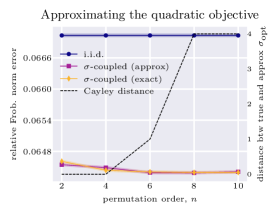
Figure 7: Relative Frobenius norm error (normalised by i.i.d. result) with permutations of order $n$ learned using exact and approximate objectives. ‘Cayley distance’ shows the difference between the learned permutations. Although dropping off-diagonal terms from the objective in Eq. 47 changes the $\sigma$-coupling, it does not significantly detriment variance reduction.

Fig. 7 plots the results for GRF estimates of the $2$-regularised Laplacian kernel on the eurosis graph, comparing the approximate and exact objectives. The former can be computed efficiently but the latter is evaluated at a cost exponential in $n$, so we limit to $n=10$ and smaller. We plot the kernel approximation error (normalised by the i.i.d. result) for different permutation orders. We also plot the Cayley distance between the permutations, which measures the difference between them. As $n$ grows, the permutations become more different so we are clearly not finding the same coupling. Nonetheless, we do not see a statistically significant difference in the amount of variance reduction. This suggests that our linear proxy objective is reasonable. We defer more detailed analytic study of this curious phenomenon to future work.

How important are the approximations? This section has provided comprehensive details about the series of approximations required to make the GRF variance reduction OT problem tractable and solve it efficiently. We close by emphasising that, even if these approximations mean that we are not exactly solving the original OT problem, we clearly nonetheless obtain a computationally efficient coupling that offers much greater variance reduction compared to heuristically-motivated techniques. Analytic intractability is common in OT (Sec. 3 being an obvious exception), but fortunately this framework also equips us with a powerful arsenal of numerical tools to achieve our goal of finding effective, cheap sample couplings.

C.3.1 Addendum: towards an analytic solution to Eq. 47

To assuage any possible dissatisfaction with the $q_{1}=q_{2}$ approximation in Eq. 48, in this section we discuss progress towards solving the optimisation problem in Eq. 47 exactly. In particular, we prove that it can be solved with high probability and:

1. at a time complexity independent from the dimensionality of vectors $\{\widehat{\psi}(q^{(i,j)})\}_{q=1}^{n}$ (at the cost of the one-time pre-processing), or

2. in polynomial time in the special case $i=j$ (under mild assumptions about the distribution of the averaged projection vectors $\{\widehat{\psi}(q^{(i,i)})\}_{q=1}^{n}$).

This is possible because of the extra structure in the quadratic matching problem. A general efficient solution remains (for now) out of reach, but we hope this progress will spur further research in this direction. Note especially that independence of the time complexity from the dimensionality of $\{\widehat{\psi}(q^{(i,i)})\}_{q=1}^{n}$ means that the difficulty of the optimisation does not depend on the number of nodes $N$: a very convenient property for large graphs.

First, for clarity of exposition, we will introduce more convenient notation and important definitions. For a given $\epsilon>0$ and a vector $\mathbf{v}\in\mathbb{R}^{d}$, define the set $N_{\epsilon}(\mathbf{v})=\{\mathbf{w}\in\mathbb{R}^{d}:|\alpha_{\mathbf{v},\mathbf{w}}-\frac{\pi}{2}|\leq\epsilon\}$, where $\alpha_{\mathbf{v},\mathbf{w}}$ is an angle between $\mathbf{v}$ and $\mathbf{w}$. Then define the property of $\epsilon$-separation as follows.

Definition C.1.

For a given $\epsilon>0$, a set of vectors $\mathcal{V}$ and a vector $\mathbf{v}\in\mathcal{V}$, we say that $\mathbf{v}$ is $\epsilon$-separated in $\mathcal{V}$ if

$$N_{\epsilon}(\mathbf{v})\cap\bigcup_{\mathbf{x}\in\mathcal{V}\backslash\{\mathbf{v}\}}N_{\epsilon}(\mathbf{x})=\emptyset.$$ (49)

Simplifying notation, we can rewrite Eq. 47 as the following optimisation problem:

$$\sigma^{*}=\textrm{argmin}_{\sigma}\sum_{q_{1},q_{2}\in\{1,...,n\}}[(\mathbf{v}_{q_{1}}^{(i)}+\mathbf{v}_{\sigma(q_{1})}^{(i)})^{\top}(\mathbf{v}_{q_{2}}^{(j)}+\mathbf{v}_{\sigma(q_{2})}^{(j)})]^{2},$$ (50)

where $\sigma$ is the permutation of the sequence $(1,2,...,n)$ and $\mathbf{v}_{q}^{(i,j)}\coloneqq\widehat{\psi}(q^{(i,j)})$. With every permutation $\sigma$ of the sequence $(1,...,n)$, we will associate the perfect matching $M(\sigma)$ in its corresponding bipartite graph with monochromatic classes of size $n$ each. Denote

$$\mathbf{f}^{(i)}_{M(\sigma)}\coloneqq\sum_{e\in M(\sigma)}\mathbf{u}_{e}^{(i)},$$ (51)

where $\mathbf{u}_{e}$ is given by

$$\mathbf{u}_{(k,\sigma(k))}^{(i)}=\textrm{vec}\left[(\mathbf{v}_{k}^{(i)}+\mathbf{v}^{(i)}_{\sigma(k)})\otimes(\mathbf{v}_{k}^{(i)}+\mathbf{v}_{\sigma(k)}^{(i)})\right].$$ (52)

Here, $\otimes$ represents the outer product and vec is the ‘vectorising’ operation that flattens its input to a vector. Note that that $\mathbf{u}_{(k,\sigma(k))}\in\mathbb{R}^{N^{2}}$.

It is straightforward to see that, in this notation, the optimisation problem becomes

$$\sigma^{*}=\textrm{argmin}_{\sigma}{\mathbf{f}^{(i)}_{M(\sigma)}}^{\top}\mathbf{f}^{(j)}_{M(\sigma)}.$$ (53)

We will now discuss progress towards solving this efficiently.

Making the problem independent of $N$. Let us first show how we can make the optimisation problem independent of the number of nodes $N$ with high probability, at the cost of a one-time pre-processing. Our basic approach is to conduct dimensionality reduction of the vectors $\mathbf{u}^{(i,j)}_{e}$ via the Johnson-Lindenstrauss Transform (JLT) [Dasgupta and Gupta, 2003]. Specifically, we compute

$$\widehat{\mathbf{u}}^{(i,j)}_{(k,\sigma(k))}=\frac{1}{\sqrt{r}}\mathbf{G}\mathbf{u}^{(i,j)}_{(k,\sigma(k))},$$ (54)

where $r\in\mathbb{N}$ denotes the number of random projections and $\mathbf{G}\in\mathbb{R}^{r\times N^{2}}$ is a Gaussian matrix with entries taken independently at random from $\mathcal{N}(0,1)$. From the well-known properties of JLT [Dasgupta et al., 2010], we have that

$$\mathbb{E}[(\widehat{\mathbf{u}}^{(i)}_{(k,\sigma(k))})^{\top}\widehat{\mathbf{u}}^{(j)}_{(k,\sigma(k))}]=(\mathbf{u}^{(i)}_{(k,\sigma(k))})^{\top}\mathbf{u}^{(j)}_{(k,\sigma(k))}$$ (55)

since it is unbiased. We also have that

$$1-\epsilon\leq\frac{\|\widehat{\mathbf{u}}^{(i)}_{(k,\sigma(k))}\pm\widehat{\mathbf{u}}^{(j)}_{(k,\sigma(k))}\|^{2}_{2}}{|\mathbf{u}^{(i)}_{(k,\sigma(k))}\pm\mathbf{u}^{(j)}_{(k,\sigma(k))}|^{2}_{2}}\leq 1+\epsilon,$$ (56)

with $r=\mathcal{O}(\frac{\log(n)}{\epsilon^{2}})$ random projections, with probability $p=1-\textrm{neg}(n)$. Here, neg denotes the negligible function of $n$.

Eq. 56 describes the ability of the JLT to (approximately) preserve $L_{2}$-norms. The analogous property for preservation of dot-products also holds, which of interest to us given Eq. 53. It follows because for any $\mathbf{x},\mathbf{y}\in\mathbb{R}^{N^{2}}$,

$$\mathbf{x}^{\top}\mathbf{y}=\frac{\|\mathbf{x}+\mathbf{y}\|^{2}-\|\mathbf{x}-\mathbf{y}\|^{2}}{4}.$$ (57)

The properties above lead us directly to an algorithm to decouple the time complexity of the optimisation from $N$. One simply replaces every $\mathbf{u}^{(i,j)}_{(k,\sigma(k))}$ with its corresponding dimensionality-reduced $\widehat{\mathbf{u}}^{(i,j)}_{(k,\sigma(k))}$ for $r=O(\frac{\log(n)}{\epsilon^{2}})$ and $\epsilon>0$ small enough. Then, by the concentration result listed above and the union bound over all pairs $(i,j)$, we conclude that the optimal $\sigma$ (potentially not unique) will remain optimal after applying the JLT (since all dot-products are approximately preserved). This completes the analysis. We stress that $r$ does not depend directly on the dimensionality of $\mathbf{u}^{(i,j)}_{(k,\sigma(k))}$, and therefore on $N$.

Polynomial in $n$ algorithm for $i=j$. We can make further progress in the special case that $i=j$, i.e. if we are minimising the variance of diagonal kernel entries $k(v_{i},v_{i})$. Denote by $T(n)$ time complexity of an efficient polynomial-time algorithm for solving the minimum weights matching problem on bipartite graphs with monochromatic parts of size $n$ each. The following is true.

Lemma C.2.

If Eq. 50 has a unique solution $\sigma^{*}$ and furthermore $\mathbf{f}_{M(\sigma^{*})}$ is $\epsilon$-separated in $\mathcal{F}=\{\mathbf{f}_{M(\sigma)}:\sigma\in S_{n}\}$ for some $0<\epsilon<\frac{\pi}{2}$ (where $S_{n}$ denotes the set of all permutations of the sequence $(1,...,n)$), then, for any $k>0$, $\sigma^{*}$ can be found in time $k\cdot T(n)$ with probability $1-(1-p_{\epsilon})^{k}$. Here, $p_{\epsilon}$ is given by the following formula:

$$p_{\epsilon}=\mathbb{P}\left[\left|\arccos\left(\frac{g_{1}}{\sqrt{g_{1}^{2}+...+g_{N^{2}}^{2}}}\right)-\frac{\pi}{2}\right|\leq\epsilon\right],$$ (58)

with $\mathbf{g}\in\mathbb{R}^{N^{2}}$ a random isotropic vector.

Proof of Lemma C.2. If $i=j$, the expression in Eq. 53 is simply $\|\mathbf{f}_{M(\sigma)}\|_{2}^{2}$. Thus, the goal is to find a permutation $\sigma$ that minimises the $L_{2}$-norm of the vector $\mathbf{f}_{M(\sigma)}$. We propose the following algorithm. At every iteration, replace each vector $\mathbf{u}_{e}$ with the projection $u_{e}=\mathbf{u}_{e}^{\top}\mathbf{g}$ for $\mathbf{g}\in\mathcal{N}(0,\mathbf{I}_{N^{2}})$. Note that, from $\epsilon$-separability, we have that if $\mathbf{g}\in N_{\epsilon}(\mathbf{v})$, then the permutation $\sigma$ corresponding to the minimum weight matching in the bipartite graph with weights given by $u_{e}$ is also equal to $\sigma^{*}$. This captures the intuition that the shortest vector will have the smallest projection on a random vector that is almost perpendicular to it, provided none of the other vectors are also almost perpendicular to this projection direction. From the fact that $\mathbf{g}$ is taken from the isotropic distribution, we know that the probability that $\mathbf{g}\in N_{\epsilon}(\mathbf{v})$ is exactly $p_{\epsilon}$, where $p_{\epsilon}$ is a geometrical constant that depends only on $N$. Our algorithm solves the projected minimum weight matching problem (in time $T(n)$) at every iteration and stores the solution $\sigma$. Vectors $\mathbf{g}$ at different iterations are chosen independently. After $k$ iterations, the algorithm computes the original objective for every previously-obtained solution and selects the one with the smallest value. From the above, this returns the optimal permutation $\sigma^{*}$ with probability $1-(1-p_{\epsilon})^{k}$, which completes the proof. ∎

Appendix D Asymptotic optimality of permutation densities for variance reduction

In Sec. 4.1 of the main text, we alluded to the choice of permutation densities in Eq. 14 being not only convenient (in terms of ease of sampling and optimising), but also well-motivated by results from OT theory. Here, we make this statement concrete, showing that in the limit of infinite permutation order $n$ this class contains the solution to a broad range of OT problems.

Theorem D.1 (Asymptotic optimality of permutation densities).

Consider the class of joint measures $\Lambda^{(\sigma)}\coloneqq\{\mu^{(\sigma)}\}$ specified by permutations $\sigma$ of order $n$, given by permutation densities from Eq. 14 pushed forward coordinate-wise using the (left-continuous) inverse CDF $F_{\eta}^{-1}$. Suppose also that the marginal measure $\eta$ is absolutely continuous with respect to Lebesgue measure. Consider also a continuous function $f:\mathbb{R}\to\mathbb{R}$ whose expectation is to be estimated using $m=2$ coupled samples. In the limit $n\to\infty$, the class $\Lambda^{(\sigma)}$ contains measures that converge weakly to the optimal transport plan – that is, the sample coupling which provides the smallest possible estimator variance.

Proof. Consider the set $\{u_{i}\coloneqq\frac{1}{n}\left(i-\frac{1}{2}\right)\}_{i=1}^{n}$ for some $n\in\mathbb{N}$. Consider also a random variable $X$ with measure $\eta\in\mathcal{P}(\mathbb{R})$ and corresponding distribution function $F$. Define its left-continuous inverse $F^{-1}(y)\coloneqq\inf\{x\in\mathbb{R}:F(x)\geq y\}$. Given some permutation order $n\in\mathbb{N}$, consider the set

$$\left\{x_{i}\coloneqq F^{-1}\left(u_{i}\right)=F^{-1}\left(\frac{i-\frac{1}{2}}{n}\right)\right\}_{i=1}^{n}$$ (59)

which we will refer to as the quantile midpoints. Then consider the discrete measure

$$\eta_{n}\coloneqq\frac{1}{n}\sum_{i=1}^{n}\delta_{x_{i}}$$ (60)

where $\delta_{x_{i}}(A)=1$ if $x_{i}\in A$ and $0$ otherwise (with $A\subset\mathbb{R}$). Denote by $F_{n}$ the distribution associated with $\eta_{n}$. Clearly, $\eta_{n}\to\eta$ weakly as $n\to\infty$ since $F_{n}(x)\to F(x)$ for any continuity point $x$ of $F$ [Billingsley, 2013]. In this sense, the measure $\eta_{n}$ is a discrete approximation to $\eta$.

Now consider the variance reduction OT problem for estimating $\mathbb{E}_{\omega\sim\eta}[f(\omega)]$ with $m=2$ samples,

$$\mu^{*}=\textrm{arg inf}_{\mu\in\Lambda_{2}(\eta)}\left[\mathbb{E}_{(\omega_{1},\omega_{2})\sim\mu}f(\omega_{1})f(\omega_{2})\right].$$ (61)

Solving this analytically for arbitrary $f$ is not in general tractable. On the other hand, if we instead take the discretised marginals $\eta_{n}$, we must solve

$$\mu_{n}^{*}=\textrm{arg inf}_{\mu\in\Lambda_{2}(\eta_{n})}\left[\mathbb{E}_{(\omega_{1},\omega_{2})\sim\mu}f(\omega_{1})f(\omega_{2})\right].$$ (62)

This special case of discrete marginal measures where all points have equal mass can be solved exactly. Our discussion is based on the proof outlined in the introduction to Villani [2021], to which the interested reader is directed for full details.

OT with equal-mass discrete marginal measures. Any measure in $\Lambda_{2}(\eta_{n})$ can be represented as a bistochastic $n\times n$ matrix $\mathbf{B}=[B_{ij}]_{i,j=1}^{N}\in\mathcal{B}_{n}$, meaning that all $B_{ij}$ are nonnegative and satisfy

$$\sum_{i}B_{ij}=1\;\forall\;j;\quad\sum_{j}B_{ij}=1\;\forall\;i.$$ (63)

Therefore, the Kantorovich problem reduces to

$$\inf_{B\in\mathcal{B}_{n}}\left[\frac{1}{n}\sum_{ij}B_{ij}C_{ij}\right]$$ (64)

where we have encoded the transport costs in the cost matrix $\mathbf{C}=[f(x_{i})f(x_{j})]_{i,j=1}^{n}$. $B_{ij}$ is interpreted as the mass of the singleton $(x_{i},x_{j})$. This is a linear minimisation problem on a convex bounded set. It is well known that a solution always exists and corresponds to the convex hull of optimal permutation matrices. In more detail: by Choquet’s theorem the problem admits solutions which are at the extremal points of $\mathcal{B}_{n}$ (points that cannot be written as a nontrivial linear combination of other points in $\mathcal{B}_{n}$). By Birkhoff’s theorem these are exactly the permutation matrices $\mathbf{B}^{(\sigma)}\coloneqq[\delta_{\sigma(i)j}]_{i,j=1}^{n}$ with $\sigma\in S_{n}$. So the optimal discrete coupling is the convex hull of the discrete joint measures corresponding to the set of optimal permutations. See the work of Villani [2021] for further details. Choosing just one of these optimal permutations $\sigma$ (since any convex combination of the corresponding measures will give the same amount of variance reduction), we have that

$$\mu_{n}^{*}=\mu_{n}^{(\sigma)}\coloneqq\sum_{i=1}^{n}\frac{1}{n}\delta_{(x_{i},x_{\sigma(i)})}.$$ (65)

Stability of OT plans. Another important result in optimal transport is the stability of transference plans: namely, that if $\eta_{n}\to\eta$ weakly then the optimal coupling $\pi_{n}\in\Lambda_{2}(\eta_{n})$ also converges to the optimal $\pi\in\Lambda_{2}(\eta)$ weakly provided the cost function $c(X_{i},X_{j})$ (in our case $f(X_{i})f(X_{j})$) is continuous and

$$\limsup_{n\to\infty}\int c(x_{1},x_{2})\textrm{d}\pi_{n}(x,y)<\infty.$$ (66)

This important observation underpins the effectiveness of numerical approximations to optimal transport. We direct the reader to Thm. 1.7.2 by Panaretos and Zemel [2020] for a proof sketch and Thm. 5.20 by Villani et al. [2009] for more detailed exposition. It follows that $\mu_{n}^{*}$ converges weakly to the true optimal coupling $\mu^{*}$.

The OT plan is (asymptotically) in our search class. Lastly, we have that our search class of couplings $\Lambda^{(\sigma)}$ (corresponding to permutation densities from Eq. 14 pushed forward by $F_{\eta}^{-1}$) contains measures that converge in distribution to $\mu_{n}^{(\sigma)}$ when $n\to\infty$. In this mathematical sense, the asymptotic limit the class of couplings amongst which we optimise includes measures that give the greatest possible variance reduction: more glibly, our method is ‘asymptotically optimal’. This is intuitive because as the order of the permutation grows each ‘tile’ of nonzero density narrows and can be increasingly well-approximated by a delta function.

To see this, consider the measure on $[0,1]^{2}$ described by the permutation density $p_{\sigma}(x,y)=n1_{\sigma(\lceil nx\rceil)=\lceil ny\rceil}$. Consider also the discrete measure on $[0,1]^{2}$ given by $\frac{1}{n}\sum_{i=1}^{n}\delta_{u_{i}}$ with the set $\{u_{i}\}_{i=1}^{n}$ the quantile midpoints defined previously. These measures converge in distribution (their corresponding joint CDFs can differ by at most $\frac{1}{n}$ at any point, which goes to $0$ as $n\to\infty$). They will also converge in distribution when pushed forward coordinate-wise by $F_{\eta}^{-1}$ by continuity of $\eta$. It follows that at asymptotic $n$ $\mu_{n}^{(\sigma)}$ and $\mu^{(\sigma)}$ converge in distribution, which completes the proof. ∎

We remark that not all the assumptions in Thm. D.1 hold in the GRF setting. In particular, neither the marginal measure $\eta$ nor the function $f$ is continuous. The intention of including Thm. D.1 is to build intuition for the reader and provide some motivation for our choice of permutation densities. We defer a rigorous investigation into relaxing these restrictive assumptions – a tough measure-theoretic problem – to future work.

Appendix E Estimating PageRank

In this appendix, we demonstrate a further use of the variance reduction OT techniques developed for graph random walks in Sec. 4: estimating the PageRank vector [Page et al., 1998]. This popular measure of the relative importance of the nodes $\mathcal{N}$ of a graph is expensive to compute exactly so is often estimated by sampling random walks [Fogaras et al., 2005]. We will show that OT can be used to find a coupling between the walks to reduce the estimator variance, demonstrating the versatility of our approach beyond improving RFs.

E.1 Setup: estimating PageRank with random walks

The PageRank vector is the stationary distribution of Markov chain whose state space is the set of all graph nodes $\mathcal{N}$, with a transition matrix

$$\widetilde{\mathbf{P}}\coloneqq(1-p)\mathbf{P}+\frac{p}{N}\mathbf{E}.$$ (67)

Here, $p\in(0,1)$ is a scalar, $N$ is the number of nodes and $\mathbf{E}=[1]_{i,j\in\mathcal{N}}$ is a matrix whose entries are all ones. $\mathbf{P}$ is the transiton matrix of a simple random walk,

$$P_{ij}=\begin{cases}\frac{1}{d_{i}}&$if $(i,j)\in\mathcal{E}\\ 0&$otherwise$\end{cases}$$ (68)

with $d_{i}$ the degree of the $i$th node. Since $\smash{\widetilde{\mathbf{P}}}$ is stochastic, aperiodic and irreducible, we define the unique PageRank vector $\bm{\rho}\in\mathbb{R}^{N}$:

$$\bm{\rho}^{\top}\widetilde{\mathbf{P}}=\bm{\rho}^{\top},\hskip 8.53581pt\bm{\rho}^{\top}\bm{1}=1,$$ (69)

where we normalised the sum of vector entries to $1$. Computing $\bm{\rho}$ analytically is expensive. Rearranging and Taylor expanding $(1-(1-p)\mathbf{P})^{-1}$, it is straightforward to see that

$$\bm{\rho}_{i}=\frac{p}{N}\sum_{j\in\mathcal{N}}\sum_{k=0}^{\infty}(1-p)^{k}\mathbf{P}^{k}_{ji}.$$ (70)

This is simply a sum over all walks from each of the graph nodes $v_{j}$ to node $v_{i}$, weighted by their respective probabilities – that is, the expected number of random walkers ending at node $v_{i}$ if they terminate with probability $p$ at every timestep – which invites the estimator proposed by Fogaras et al. [2005],

$$\widehat{\bm{\rho}}_{i}=\frac{1}{Nm}\sum_{v_{j}\in\mathcal{N}}\sum_{n=1}^{m}\mathbb{I}[n\textrm{th walk from node }v_{j}\textrm{ terminates at node}\hskip 2.84526ptv_{i}].$$ (71)

An interesting and practically important question is whether the variance of the estimator $\widehat{\bm{\rho}}$ can be improved by coupling random walks. As with GRFs, this can be achieved using antithetic termination [Reid et al., 2024c] (see Sec. C.2). However, we will see that our OT length coupling approach does equally well or better.

E.2 OT formulation of PageRank variance reduction

Given $m=2$ walks, the variance of the PageRank estimator $\textrm{Var}(\widehat{\bm{\rho}}_{i})$ depends on the quantity

$$\begin{multlined}\mathbb{E}(\widehat{\bm{\rho}}_{i}^{2})=\mathbb{E}\left[\frac{1}{N^{2}m^{2}}\sum_{v_{j},v_{k}\in\mathcal{N}}\sum_{n_{1},n_{2}=1}^{2}\mathbb{I}[n_{1}\textrm{th walk from node }v_{j}\textrm{ terminates at node}\hskip 2.84526ptv_{i}]\right.\\ \left.\cdot\mathbb{I}[n_{2}\textrm{th walk from node }v_{k}\textrm{ terminates at node}\hskip 2.84526ptv_{i}]\right].\end{multlined}\mathbb{E}(\widehat{\bm{\rho}}_{i}^{2})=\mathbb{E}\left[\frac{1}{N^{2}m^{2}}\sum_{v_{j},v_{k}\in\mathcal{N}}\sum_{n_{1},n_{2}=1}^{2}\mathbb{I}[n_{1}\textrm{th walk from node }v_{j}\textrm{ terminates at node}\hskip 2.84526ptv_{i}]\right.\\ \left.\cdot\mathbb{I}[n_{2}\textrm{th walk from node }v_{k}\textrm{ terminates at node}\hskip 2.84526ptv_{i}]\right].$$ (72)

After a few lines of algebra, the OT problem to minimise this quantity is

$$\begin{multlined}\mu^{*}=\arg\inf_{\mu\in\Lambda_{2}(\eta_{\textrm{G}})}\mathbb{E}_{(l_{1},l_{2})\sim\mu}\sum_{v_{j}\in\mathcal{N}}\mathbb{P}[\textrm{RW of length $l_{1}$ from node $v_{j}$ terminates at node $v_{i}$}]\\ \cdot\mathbb{P}[\textrm{RW of length $l_{2}$ from node $v_{j}$ terminates at node $v_{i}$}]\end{multlined}\mu^{*}=\arg\inf_{\mu\in\Lambda_{2}(\eta_{\textrm{G}})}\mathbb{E}_{(l_{1},l_{2})\sim\mu}\sum_{v_{j}\in\mathcal{N}}\mathbb{P}[\textrm{RW of length $l_{1}$ from node $v_{j}$ terminates at node $v_{i}$}]\\ \cdot\mathbb{P}[\textrm{RW of length $l_{2}$ from node $v_{j}$ terminates at node $v_{i}$}]$$ (73)

without making any approximations. $\mathbb{P}(\cdot)$ denotes the probability of the event in brackets. As with GRFs, for tractability we restrict our search space of joint distributions to permutation densities pushed forward coordinate-wise with the geometric distribution inverse CDF, and this becomes

$$\begin{multlined}\sigma^{*}=\arg\inf_{\sigma}\sum_{v_{j}\in\mathcal{N}}\sum_{q\in[\![n]\!]}\mathbb{P}[\textrm{RW with length in $q$th quadrant from node $v_{j}$ terminates at node $v_{i}$}]\\ \cdot\mathbb{P}[\textrm{RW with length in $\sigma(q)$th quadrant from node $v_{j}$ terminates at node $v_{i}$}].\end{multlined}\sigma^{*}=\arg\inf_{\sigma}\sum_{v_{j}\in\mathcal{N}}\sum_{q\in[\![n]\!]}\mathbb{P}[\textrm{RW with length in $q$th quadrant from node $v_{j}$ terminates at node $v_{i}$}]\\ \cdot\mathbb{P}[\textrm{RW with length in $\sigma(q)$th quadrant from node $v_{j}$ terminates at node $v_{i}$}].$$ (74)

The probabilities can be efficiently estimated by simulating random walks on the graph and recording where they terminate. This leaves us with a minimum-weights bipartite matching problem which can as usual be solved efficiently with the Hungarian algorithm [Kuhn, 1955].

Note that we made fewer simplifications than for GRFs (Sec. C.1). They only requirements for tractability are restricting the class of considered joints to $\sigma$-couplings and computing MC estimates of the terms in the OT cost matrix. We do not need to e.g. move $\mathbb{E}_{\textrm{dirs}}$ inside a square or approximate a quadratic matching problem by a linear-weights counterpart.

E.3 Empirical results for PageRank

Figure 8: PageRank estimator errors $\|\bm{\rho}-\widehat{\bm{\rho}}\|_{2}$ for a range of real-world graphs when $2$ random walkers are taken to be i) i.i.d., ii) antithetic or iii) $\sigma$-coupled. Lower is better. The error is always at least as small and often substantially better when the walkers are coupled using our OT coupling. Estimates of one standard deviation are shaded.

We now provide experiments using our OT coupling to improve the convergence of PageRank estimates. Fig. 8 shows the results. For termination probabilities $p\in\{0.1,0.2,0.3,0.4,0.5,0.6,0.7,0.8,0.9\}$, we compute the optimal permutation $\sigma$ by solving the matching problem in Eq. 74 on an Erdős-Rènyi graph with $N=100$ nodes, taking permutation order $n=10$ as a hyperparameter. We then test these couplings on a range of real-world graphs [Ivashkin, 2023] of different sizes, plotting the estimator error $\|\bm{\rho}-\widehat{\bm{\rho}}\|_{2}$ (where $\bm{\rho}$ is the true PageRank vector and $\widehat{\bm{\rho}}$ is its MC estimate) against the termination probability $p$. We include walkers that are i.i.d., antithetic [Reid et al., 2024c] and $\sigma$-coupled. At every value of $p$, our method performs at least as well as the baselines, and in some cases (e.g. on the very large cora graph) it gives much greater variance reduction.

Note that we only consider connected subgraphs and take $1000$ repeats to estimate the standard deviations. Reading the plots from left to right for the top row and then the bottom, the number of nodes are: $\{34,62,105,115,398,986,1133,1272,2120,2708\}$. The shape of the curve and size of the gain from coupling depends on the particular graph being considered. For some graphs it is not possible to obtain a big reduction in PageRank estimator variance by coupling walkers (e.g. football and newsgroup), so neither antithetic termination nor our $\sigma$-coupling can provide a big gain. A detailed investigation of how these observations relate to the mathematical graph structure is deferred to future work.

Appendix F GRFs for GPs: additional details and experimental results

In this appendix, we supplement Sec. 4.2 by providing further experimental results for GRFs, including Gram matrix estimation on a wider range of graphs and a scalable graph-based GP on a different real-world dataset. We also provide technical background and tedious details considered too long for inclusion in the main text.

F.1 More results for Gram matrix estimation

First, we run the experiment in the first part of Sec. 4.2 for more real-world graphs. We approximate the $2$-regularised Laplacian kernel $\smash{(\mathbf{I}-\sigma^{2}\widetilde{\mathbf{L}})^{-2}}$ with a regularisation parameter $\sigma=1$ and $m=2$ walkers. Fig. 9 shows the results, with the kernel approximation error normalised by the i.i.d. result (unlike in Fig. 1) for clarity of comparison. The $\sigma$-coupling consistently reduces the estimator variance, providing equally good or better results compared to the hand-crafted antithetic termination algorithm. The size of the gain depends on the graph structure. More work is needed to characterise the type of graph for which coupling walk lengths gives the biggest reductions in kernel estimator error.

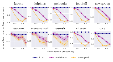
Figure 9: Relative Frobenius norm error $\|\mathbf{K}-\widehat{\mathbf{K}}\|_{\textrm{F}}/\|\mathbf{K}\|_{\textrm{F}}$ between true and approximated Gram matrices for different termination probabilities when walkers are i) i.i.d., ii) antithetic [Reid et al., 2024c] or iii) $\sigma$-coupled using our OT approach. All results are normalised by the i.i.d. variance for easy comparison. Lower is better. The $\sigma$-coupling is consistently as good or better across values of $p$ and graph topologies and sizes. Standard deviation estimates are shaded.

F.2 Scalable GPs on graphs

A very short introduction to graph-based GPs. In certain applications of Gaussian processes, kernels based on Euclidean distance are unsuitable – e.g. when predicting traffic congestion since locations that are spatially close may not be connected by roads. Kernels defined on the nodes of a graph $\mathcal{G}$ may be more appropriate, giving structured covariance matrices that encode the dependence between pairs of vertices. We can then perform inference and make predictions using GPs on graphs [Borovitskiy et al., 2021, Zhi et al., 2023].

Like their Euclidean counterparts, exact GPs on graphs suffer $\mathcal{O}(N^{3})$ time complexity, making them impractical for very large structures. Techniques to improve their scalability include graph Fourier feature approximations, which approximate the kernel matrix using a truncated eigenvalue expansion computed using the Lanczos algorithm.  The price of increased speed is that our kernel estimate is biased. Another approach is to restrict to kernels whose inverses are sparse, e.g. a Matérn kernel with a small integer $\nu$-parameter, at the expense of lost flexibility [Borovitskiy et al., 2021]. In this paper, we have proposed to instead use GRFs, which give an unbiased estimate to the kernel matrix in subquadratic time. GRFs are sparse: intuitively, $\phi_{\textrm{GRF}}(v_{i})$ is constructed by simulating $m$ random walks out of $v_{i}$ and adding weighted contributions only at the coordinates corresponding to visited nodes. For walks with geometrically-distributed lengths this is typically a small subset of $\mathcal{N}$. Therefore, the matrix $\smash{\widehat{\mathbf{K}}\coloneqq[\phi(v_{i})^{\top}\phi(v_{j})]_{i,j=1}^{N}}$ is a sparse, unbiased estimate to any kernel, not just specific families. We can use established numerical routines for sparse linear algebra to speed up training, providing computational savings on big graphs. This is analagous to the sparse spectrum GPs discussed in App. B [Lázaro-Gredilla et al., 2010]; the interested reader might benefit from reviewing this section first.

Our contribution to scalable graph-based GPs. Using GRFs for scalable approximate inference on graphs is itself a novel contribution that deserves detailed exploration in future work. Since our central goal is to use perspectives from OT to improve the convergence of GRFs, we confine our focus to the question: can coupled random walks give more accurate estimates of graph GP posteriors? We defer a detailed comparison of our method to other scalable graph-based GP techniques to a future self-contained paper.

Training GRF-GPs: technical details. Here, provide details to supplement Sec. 4.2. We use mesh graphs made available by Dawson-Haggerty [2023], taking the faces as our graph nodes. Reading left to right, the number of nodes are: $894,999,1280,1572,3838,8700$. For probabilistic mesh interpolation, we use the diffusion kernel $\mathbf{K}=\kappa\exp(-\gamma^{2}\widetilde{\mathbf{L}})$. Here, $\widetilde{\mathbf{L}}$ is the normalised graph Laplacian (Eq. 40) and $\kappa,\gamma$ are learnable parameters corresponding to the signal variance and kernel lengthscale respectively. The observation noise $\sigma$ is also learnable. For every graph, we construct a kernel estimate by sampling $m=8$ i.i.d. random walks out of every node. We then train the corresponding vanilla GP by optimising the log marginal likelihood on observed nodes, using the Adam optimiser [Kingma and Ba, 2014] for $1000$ epochs (after which both the objective value and the hyperparameters are empirically found to have converged). We freeze $\kappa,\gamma,\sigma$ and compute the corresponding exact kernel. We approximate this exact kernel using $\{16,32,64\}$ random walks that are either i.i.d., antithetic or $\sigma$-coupled. We perform approximate Bayesian inference in each case, computing the accuracy of the kernel estimate, the average test RMSE and the KL divergence to the true posterior distribution (unnormalised by the number of test points). We use permutations of order $n=50$ and a termination probability $p=0.4$. As reported in the main body, coupling the lengths of graph random walkers permits better approximate Bayesian inference with GPs on graphs.

F.3 Probabilistic traffic interpolation

In this section, we provide further details about the final experiment of Sec. 4.2, which uses a scalable graph-based GP to predict traffic flow speeds on the highways of San Jose, California.

Dataset. Readers are directed to the original paper [Borovitskiy et al., 2021] for exhaustive details about the dataset curation and graph computation. Here, we simply remark that this graph is sufficiently large that exact GP methods become slow ($N=1016$), and observations are only made at a small subset of the nodes ($325$) so good uncertainty quantification is essential.

Results for GRFs. We randomly divide the nodes into training and test datasets of sizes $N_{\textrm{train}}=250$ and $N_{\textrm{test}}=75$ respectively. As described in App. F.2, we train a scalable GRF-GP with $m=8$ i.i.d. walkers set up to approximate the diffusion kernel, optimising the training data negative log marginal likelihood. Next, we freeze the kernel and noise parameters, and compare the performance of GRFs with $m\in\{4,8,16\}$ i.i.d., antithetic [Reid et al., 2024c] and $\sigma$-coupled walkers. As before, we consider the quality of Gram matrix approximation, the accuracy of predictions (test RMSE) and the quality of the predictive uncertainties (KL divergence to true posterior). Fig. 10 shows the results. $\sigma$-GRFs consistently do best on all metrics, even with a severely restricted sampling budget.

Figure 10: Results for probabilistic traffic interpolation experiment. Plots show the kernel approximation accuracy, test RMSE and KL divergence to the true posterior for graph kernels estimated using i.i.d., antithetic and $\sigma$-coupled GRFs. Lower is better. $\sigma$-coupling gives the best results for approximate inference. Estimates of the standard deviation over random draws of walkers are shaded.

References

- Alon et al. (2007) Noga Alon, Itai Benjamini, Eyal Lubetzky, and Sasha Sodin. Non-backtracking random walks mix faster. Communications in Contemporary Mathematics, 9(04):585–603, 2007. URL https://doi.org/10.1142/S021919970700255.
- Avron et al. (2017a) Haim Avron, Michael Kapralov, Cameron Musco, Christopher Musco, Ameya Velingker, and Amir Zandieh. Random fourier features for kernel ridge regression: Approximation bounds and statistical guarantees. In International conference on machine learning, pages 253–262. PMLR, 2017a. URL https://doi.org/10.48550/arXiv.1804.09893.
- Avron et al. (2017b) Haim Avron, Michael Kapralov, Cameron Musco, Christopher Musco, Ameya Velingker, and Amir Zandieh. Random fourier features for kernel ridge regression: Approximation bounds and statistical guarantees. In Proceedings of the 34th International Conference on Machine Learning, ICML 2017, Sydney, NSW, Australia, 6-11 August 2017, volume 70 of Proceedings of Machine Learning Research, pages 253–262. PMLR, 2017b. URL http://proceedings.mlr.press/v70/avron17a.html.
- Bhat and Mondal (2021) Chandra R Bhat and Aupal Mondal. On the almost exact-equivalence of the radial and spherical unconstrained choleskybased parameterization methods for correlation matrices. Technical report, Department of Civil, Architectural and Environmental Engineering, The University of Texas at Austin, 2021. URL https://repositories.lib.utexas.edu/server/api/core/bitstreams/69c04b9a-2175-4392-b7b0-a8f5445ad405/content.
- Billingsley (2013) Patrick Billingsley. Convergence of probability measures. John Wiley & Sons, 2013.
- Bojarski et al. (2017) Mariusz Bojarski, Anna Choromanska, Krzysztof Choromanski, Francois Fagan, Cedric Gouy-Pailler, Anne Morvan, Nouri Sakr, Tamas Sarlos, and Jamal Atif. Structured adaptive and random spinners for fast machine learning computations. In Artificial intelligence and statistics, pages 1020–1029. PMLR, 2017. URL https://doi.org/10.48550/arXiv.1610.06209.
- Borovitskiy et al. (2021) Viacheslav Borovitskiy, Iskander Azangulov, Alexander Terenin, Peter Mostowsky, Marc Deisenroth, and Nicolas Durrande. Matérn gaussian processes on graphs. In International Conference on Artificial Intelligence and Statistics, pages 2593–2601. PMLR, 2021. URL https://doi.org/10.48550/arXiv.2010.15538.
- Campbell (2002) Colin Campbell. Kernel methods: a survey of current techniques. Neurocomputing, 48(1-4):63–84, 2002. URL https://doi.org/10.1016/S0925-2312(01)00643-9.
- Canu and Smola (2006) Stéphane Canu and Alex Smola. Kernel methods and the exponential family. Neurocomputing, 69(7-9):714–720, 2006. URL https://doi.org/10.1016/j.neucom.2005.12.009.
- Chapelle et al. (2002) Olivier Chapelle, Jason Weston, and Bernhard Schölkopf. Cluster kernels for semi-supervised learning. Advances in neural information processing systems, 15, 2002. URL https://dl.acm.org/doi/10.5555/2968618.2968693.
- Chen et al. (2001) Chao Chen, Karl Petty, Alexander Skabardonis, Pravin Varaiya, and Zhanfeng Jia. Freeway performance measurement system: mining loop detector data. Transportation research record, 1748(1):96–102, 2001. URL https://api.semanticscholar.org/CorpusID:108891582.
- Chi et al. (2019) Jinjin Chi, Jihong Ouyang, Ximing Li, Yang Wang, and Meng Wang. Approximate optimal transport for continuous densities with copulas. In IJCAI, pages 2165–2171, 2019. URL https://www.ijcai.org/proceedings/2019/0300.pdf.
- Choromanski et al. (2018) Krzysztof Choromanski, Mark Rowland, Tamás Sarlós, Vikas Sindhwani, Richard Turner, and Adrian Weller. The geometry of random features. In International Conference on Artificial Intelligence and Statistics, pages 1–9. PMLR, 2018. URL http://proceedings.mlr.press/v84/choromanski18a/choromanski18a.pdf.
- Choromanski et al. (2020) Krzysztof Choromanski, Valerii Likhosherstov, David Dohan, Xingyou Song, Andreea Gane, Tamas Sarlos, Peter Hawkins, Jared Davis, Afroz Mohiuddin, Lukasz Kaiser, et al. Rethinking attention with performers. arXiv preprint arXiv:2009.14794, 2020. URL https://doi.org/10.48550/arXiv.2009.14794.
- Choromanski et al. (2017) Krzysztof M Choromanski, Mark Rowland, and Adrian Weller. The unreasonable effectiveness of structured random orthogonal embeddings. Advances in neural information processing systems, 30, 2017. URL https://doi.org/10.48550/arXiv.1703.00864.
- Choromanski (2023) Krzysztof Marcin Choromanski. Taming graph kernels with random features. In International Conference on Machine Learning, pages 5964–5977. PMLR, 2023. URL https://doi.org/10.48550/arXiv.2305.00156.
- Chung (1997) Fan RK Chung. Spectral graph theory, volume 92. American Mathematical Soc., 1997.
- Cuturi (2013) Marco Cuturi. Sinkhorn distances: Lightspeed computation of optimal transport. Advances in neural information processing systems, 26, 2013. URL https://papers.nips.cc/paper_files/paper/2013/file/af21d0c97db2e27e13572cbf59eb343d-Paper.pdf.
- Dao et al. (2017) Tri Dao, Christopher M De Sa, and Christopher Ré. Gaussian quadrature for kernel features. Advances in neural information processing systems, 30, 2017. URL https://doi.org/10.48550/arXiv.1709.02605.
- Dasgupta et al. (2010) Anirban Dasgupta, Ravi Kumar, and Tamás Sarlós. A sparse johnson: Lindenstrauss transform. In Proceedings of the forty-second ACM symposium on Theory of computing, pages 341–350, 2010. URL https://doi.org/10.1145/1806689.1806737.
- Dasgupta and Gupta (2003) Sanjoy Dasgupta and Anupam Gupta. An elementary proof of a theorem of johnson and lindenstrauss. Random Struct. Algorithms, 22(1):60–65, 2003. doi: 10.1002/RSA.10073. URL https://doi.org/10.1002/rsa.10073.
- Dawson-Haggerty (2023) Michael Dawson-Haggerty. Trimesh repository, 2023. URL https://github.com/mikedh/trimesh.
- Dick et al. (2013) Josef Dick, Frances Y Kuo, and Ian H Sloan. High-dimensional integration: the quasi-monte carlo way. Acta Numerica, 22:133–288, 2013. URL https://doi.org/10.1017/S0962492913000044.
- Fogaras et al. (2005) Dániel Fogaras, Balázs Rácz, Károly Csalogány, and Tamás Sarlós. Towards scaling fully personalized pagerank: Algorithms, lower bounds, and experiments. Internet Mathematics, 2(3):333–358, 2005. URL https://doi.org/10.1007/978-3-540-30216-2_9.
- Glasserman and Yao (1992) Paul Glasserman and David D Yao. Some guidelines and guarantees for common random numbers. Management Science, 38(6):884–908, 1992. URL https://doi.org/10.1287/mnsc.38.6.884.
- Goemans and Williamson (2001) Michel X Goemans and David Williamson. Approximation algorithms for max-3-cut and other problems via complex semidefinite programming. In Proceedings of the thirty-third annual ACM symposium on Theory of computing, pages 443–452, 2001. URL https://doi.org/10.1016/j.jcss.2003.07.012.
- Halton (1960) John H Halton. On the efficiency of certain quasi-random sequences of points in evaluating multi-dimensional integrals. Numerische Mathematik, 2:84–90, 1960. URL https://doi.org/10.1007/BF01386213.
- Hammersley and Morton (1956) JM Hammersley and KW Morton. A new monte carlo technique: antithetic variates. In Mathematical proceedings of the Cambridge philosophical society, volume 52, pages 449–475. Cambridge University Press, 1956. URL https://doi.org/10.1017/S0305004100031455.
- Haugh (2016) Martin Haugh. An introduction to copulas. quantitative risk management. Lecture Notes. New York: Columbia University, 2016. URL http://www.columbia.edu/~mh2078/QRM/Copulas.pdf.
- Ivashkin (2023) Vladimir Ivashkin. Community graphs repository, 2023. URL https://github.com/vlivashkin/community-graphs.
- Johnson (1984) William B Johnson. Extensions of lipschitz mappings into a hilbert space. Contemp. Math., 26:189–206, 1984. URL http://stanford.edu/class/cs114/readings/JL-Johnson.pdf.
- Kingma and Ba (2014) Diederik P Kingma and Jimmy Ba. Adam: A method for stochastic optimization. arXiv preprint arXiv:1412.6980, 2014. URL https://doi.org/10.48550/arXiv.1412.6980.
- Kondor and Lafferty (2002) Risi Imre Kondor and John Lafferty. Diffusion kernels on graphs and other discrete structures. In Proceedings of the 19th international conference on machine learning, volume 2002, pages 315–322, 2002. URL https://www.ml.cmu.edu/research/dap-papers/kondor-diffusion-kernels.pdf.
- Kontorovich et al. (2008) Leonid Kontorovich, Corinna Cortes, and Mehryar Mohri. Kernel methods for learning languages. Theor. Comput. Sci., 405(3):223–236, 2008. doi: 10.1016/j.tcs.2008.06.037. URL https://doi.org/10.1016/j.tcs.2008.06.037.
- Kuhn (1955) Harold W Kuhn. The hungarian method for the assignment problem. Naval research logistics quarterly, 2(1-2):83–97, 1955. URL https://doi.org/10.1002/nav.3800020109.
- Lázaro-Gredilla et al. (2010) Miguel Lázaro-Gredilla, Joaquin Quinonero-Candela, Carl Edward Rasmussen, and Aníbal R Figueiras-Vidal. Sparse spectrum gaussian process regression. The Journal of Machine Learning Research, 11:1865–1881, 2010. URL https://jmlr.csail.mit.edu/papers/volume11/lazaro-gredilla10a/lazaro-gredilla10a.pdf.
- Le et al. (2013) Quoc Le, Tamás Sarlós, Alex Smola, et al. Fastfood-approximating kernel expansions in loglinear time. In Proceedings of the international conference on machine learning, volume 85, 2013. URL https://doi.org/10.48550/arXiv.1408.3060.
- Likhosherstov et al. (2022) Valerii Likhosherstov, Krzysztof M Choromanski, Kumar Avinava Dubey, Frederick Liu, Tamas Sarlos, and Adrian Weller. Chefs’ random tables: Non-trigonometric random features. Advances in Neural Information Processing Systems, 35:34559–34573, 2022. URL https://doi.org/10.48550/arXiv.2205.15317.
- Liu et al. (2022) Fanghui Liu, Xiaolin Huang, Yudong Chen, and Johan A. K. Suykens. Random features for kernel approximation: A survey on algorithms, theory, and beyond. IEEE Trans. Pattern Anal. Mach. Intell., 44(10):7128–7148, 2022. doi: 10.1109/TPAMI.2021.3097011. URL https://doi.org/10.1109/TPAMI.2021.3097011.
- Luo (2019) Siqiang Luo. Distributed pagerank computation: An improved theoretical study. In Proceedings of the AAAI Conference on Artificial Intelligence, volume 33, pages 4496–4503, 2019. URL https://doi.org/10.1609/aaai.v33i01.33014496.
- Lyu (2017) Yueming Lyu. Spherical structured feature maps for kernel approximation. In International Conference on Machine Learning, pages 2256–2264. PMLR, 2017. URL http://proceedings.mlr.press/v70/lyu17a/lyu17a.pdf.
- Morokoff and Caflisch (1995) William J Morokoff and Russel E Caflisch. Quasi-monte carlo integration. Journal of computational physics, 122(2):218–230, 1995. URL https://doi.org/10.1006/jcph.1995.1209.
- Munkhoeva et al. (2018) Marina Munkhoeva, Yermek Kapushev, Evgeny Burnaev, and Ivan Oseledets. Quadrature-based features for kernel approximation. Advances in neural information processing systems, 31, 2018. URL https://doi.org/10.48550/arXiv.1802.03832.
- Nelsen (2006) Roger B Nelsen. An introduction to copulas. Springer, 2006.
- Page et al. (1998) Lawrence Page, Sergey Brin, Rajeev Motwani, and Terry Winograd. The pagerank citation ranking: Bring order to the web. Technical report, Technical report, stanford University, 1998. URL https://www.cis.upenn.edu/~mkearns/teaching/NetworkedLife/pagerank.pdf.
- Panaretos and Zemel (2020) Victor M Panaretos and Yoav Zemel. An invitation to statistics in Wasserstein space. Springer Nature, 2020.
- Pfaff et al. (2020) Tobias Pfaff, Meire Fortunato, Alvaro Sanchez-Gonzalez, and Peter W Battaglia. Learning mesh-based simulation with graph networks. arXiv preprint arXiv:2010.03409, 2020. URL https://doi.org/10.48550/arXiv.2010.03409.
- Rahimi and Recht (2007) Ali Rahimi and Benjamin Recht. Random features for large-scale kernel machines. Advances in neural information processing systems, 20, 2007. URL https://people.eecs.berkeley.edu/~brecht/papers/07.rah.rec.nips.pdf.
- Rahimi and Recht (2008) Ali Rahimi and Benjamin Recht. Weighted sums of random kitchen sinks: Replacing minimization with randomization in learning. In Advances in Neural Information Processing Systems 21, Proceedings of the Twenty-Second Annual Conference on Neural Information Processing Systems, Vancouver, British Columbia, Canada, December 8-11, 2008, pages 1313–1320, 2008. URL https://papers.nips.cc/paper_files/paper/2008/file/0efe32849d230d7f53049ddc4a4b0c60-Paper.pdf.
- Reid et al. (2023) Isaac Reid, Krzysztof Marcin Choromanski, Valerii Likhosherstov, and Adrian Weller. Simplex random features. In International Conference on Machine Learning, pages 28864–28888. PMLR, 2023. URL https://doi.org/10.48550/arXiv.2301.13856.
- Reid et al. (2024a) Isaac Reid, Eli Berger, Krzysztof Choromanski, and Adrian Weller. Repelling random walks. In International Conference on Learning Representations, 2024a. URL https://doi.org/10.48550/arXiv.2310.04854.
- Reid et al. (2024b) Isaac Reid, Krzysztof Choromanski, Eli Berger, and Adrian Weller. General graph random features. In International Conference on Learning Representations, 2024b. URL https://doi.org/10.48550/arXiv.2310.04859.
- Reid et al. (2024c) Isaac Reid, Adrian Weller, and Krzysztof M Choromanski. Quasi-monte carlo graph random features. Advances in Neural Information Processing Systems, 36, 2024c. URL https://doi.org/10.48550/arXiv.2305.12470.
- Rowland et al. (2018) Mark Rowland, Krzysztof M Choromanski, François Chalus, Aldo Pacchiano, Tamas Sarlos, Richard E Turner, and Adrian Weller. Geometrically coupled monte carlo sampling. Advances in Neural Information Processing Systems, 31, 2018. URL https://mlg.eng.cam.ac.uk/adrian/NeurIPS18-gcmc.pdf.
- Scholkopf and Smola (2018) Bernhard Scholkopf and Alexander J Smola. Learning with kernels: support vector machines, regularization, optimization, and beyond. MIT press, 2018.
- Shen et al. (2017) Weiwei Shen, Zhihui Yang, and Jun Wang. Random features for shift-invariant kernels with moment matching. In Proceedings of the AAAI conference on artificial intelligence, volume 31, 2017. URL https://doi.org/10.1609/aaai.v31i1.10825.
- Sinkhorn and Knopp (1967) Richard Sinkhorn and Paul Knopp. Concerning nonnegative matrices and doubly stochastic matrices. Pacific Journal of Mathematics, 21(2):343–348, 1967. URL https://msp.org/pjm/1967/21-2/pjm-v21-n2-p14-s.pdf.
- Sklar (1959) M Sklar. Fonctions de répartition à n dimensions et leurs marges. In Annales de l’ISUP, volume 8, pages 229–231, 1959. URL https://hal.science/hal-04094463/document.
- Smola and Kondor (2003a) Alexander J. Smola and Risi Kondor. Kernels and regularization on graphs. In Computational Learning Theory and Kernel Machines, 16th Annual Conference on Computational Learning Theory and 7th Kernel Workshop, COLT/Kernel 2003, Washington, DC, USA, August 24-27, 2003, Proceedings, volume 2777 of Lecture Notes in Computer Science, pages 144–158. Springer, 2003a. URL https://doi.org/10.1007/978-3-540-45167-9_12.
- Smola and Kondor (2003b) Alexander J Smola and Risi Kondor. Kernels and regularization on graphs. In Learning Theory and Kernel Machines: 16th Annual Conference on Learning Theory and 7th Kernel Workshop, COLT/Kernel 2003, Washington, DC, USA, August 24-27, 2003. Proceedings, pages 144–158. Springer, 2003b. URL https://people.cs.uchicago.edu/~risi/papers/SmolaKondor.pdf.
- Smola and Schölkopf (2002) Alexander J. Smola and Bernhard Schölkopf. Bayesian kernel methods. In Advanced Lectures on Machine Learning, Machine Learning Summer School 2002, Canberra, Australia, February 11-22, 2002, Revised Lectures, volume 2600 of Lecture Notes in Computer Science, pages 65–117. Springer, 2002. URL https://doi.org/10.1007/3-540-36434-X_3.
- Thorpe (2019) Matthew Thorpe. Introduction to optimal transport. Lecture Notes, 3, 2019. URL https://www.damtp.cam.ac.uk/research/cia/files/teaching/Optimal_Transport_Notes.pdf.
- Tripp et al. (2024) Austin Tripp, Sergio Bacallado, Sukriti Singh, and José Miguel Hernández-Lobato. Tanimoto random features for scalable molecular machine learning. Advances in Neural Information Processing Systems, 36, 2024. URL https://doi.org/10.48550/arXiv.2306.14809.
- Villani (2021) Cédric Villani. Topics in optimal transportation, volume 58. American Mathematical Soc., 2021.
- Villani et al. (2009) Cédric Villani et al. Optimal transport: old and new, volume 338. Springer, 2009.
- Williams and Rasmussen (2006) Christopher KI Williams and Carl Edward Rasmussen. Gaussian processes for machine learning, volume 2. MIT press Cambridge, MA, 2006.
- Yang et al. (2014a) Jiyan Yang, Vikas Sindhwani, Haim Avron, and Michael W. Mahoney. Quasi-monte carlo feature maps for shift-invariant kernels. In Proceedings of the 31th International Conference on Machine Learning, ICML 2014, Beijing, China, 21-26 June 2014, volume 32 of JMLR Workshop and Conference Proceedings, 2014a. URL http://proceedings.mlr.press/v32/yangb14.html.
- Yang et al. (2014b) Jiyan Yang, Vikas Sindhwani, Quanfu Fan, Haim Avron, and Michael W Mahoney. Random laplace feature maps for semigroup kernels on histograms. In Proceedings of the IEEE Conference on Computer Vision and Pattern Recognition, pages 971–978, 2014b. URL https://vikas.sindhwani.org/RandomLaplace.pdf.
- Yu et al. (2016) Felix Xinnan X Yu, Ananda Theertha Suresh, Krzysztof M Choromanski, Daniel N Holtmann-Rice, and Sanjiv Kumar. Orthogonal random features. Advances in neural information processing systems, 29, 2016. URL https://doi.org/10.48550/arXiv.1610.09072.
- Zhi et al. (2023) Yin-Cong Zhi, Yin Cheng Ng, and Xiaowen Dong. Gaussian processes on graphs via spectral kernel learning. IEEE Transactions on Signal and Information Processing over Networks, 2023. URL https://doi.org/10.48550/arXiv.2006.07361.
- Zhou et al. (2015) Zhuojie Zhou, Nan Zhang, and Gautam Das. Leveraging history for faster sampling of online social networks. arXiv preprint arXiv:1505.00079, 2015. URL https://doi.org/10.48550/arXiv.1505.00079.