Entanglement and Bell inequality violation in vector diboson systems produced in decays of spin-0 particles

Abstract

We discuss entanglement and the violation of the CGLMP inequality in a system of two vector bosons produced in the decay of a spin-0 particle. We assume the most general CPT conserving, Lorentz- invariant coupling of the spin-0 particle with the daughter bosons. We compute the most general two-boson density matrix obtained by averaging over kinematical configurations with an appropriate probability distribution (which can be obtained when both bosons subsequently decay into fermion-antifermion). We show that the two-boson state is entangled and violates the CGLMP inequality for all values of the (anomalous) coupling constants and that in this case the state is entangled iff it can violate the CGLMP inequality. As an exemplary process of this kind we use the decay $H\to ZZ$ with anomalous coupling.

I Introduction

One of the most intriguing and fascinating aspects of quantum mechanics is quantum nonlocality. Nonlocality is expressed by correlations of entangled quantum states of quantum objects. As was proven theoretically by John Stuart Bell [1] nonlocality is an immanent aspect of quantum reality which was confirmed for elementary systems in series of correlation experiments in different scales of energy-momentum as well as different conditions for space-time localization [2, 3, 4, 5, 6, 7, 8, 9]. Recently, the possibility of testing nonlocality of quantum mechanics under extremal conditions arising in a decay of the Higgs boson has been put forward [10, 11, 12, 13, 14, 15, 16, 17]. Indeed, in the most interesting case of Higgs decay into two gauge bosons ($ZZ$ or $WW$) we have possibility to measure quantum spin states of unstable vector bosons. This is possible by means of registration of their decay products (leptons) which are detected in polarization states determined by kinematics. The decay process of weak bosons takes place in the extremely short time $10^{-25}$ sec and at last one of decaying bosons is in a virtual state, out of the mass shell. Therefore, investigation of possible correlations of entangled vector bosons can provide a test of quantum mechanical nonlocality under completely new conditions.

Einstein–Podolsky–Rosen (EPR) type correlation experiment with relativistic vector bosons in the simplest scalar state was considered in [18] for the first time. The possibility of observing the violation of Clauser–Horn–Shimony–Holt (CHSH) and Collins–Gisin–Linden–Massar–Popescu (CGLMP) inequalities by $WW$ bosons arising in the actual decay $H\to WW$ for the first time was analyzed in [10]. In [11] the possibility of violation of CHSH, Mermin and CGLMP inequalities by a boson-antiboson system in the most general scalar state (introduced in this context in [19]) was discussed. In [12] the entanglement and violation of CGLMP inequality by a pair of $Z$ bosons arising in the decay $H\to ZZ$ was considered. The authors of [12] assumed the Standard Model interaction of $H$ with the daughter $Z$ bosons and showed that $ZZ$ state produced in such a process is highly entanglement. In our paper [16] we also discussed entanglement and the violation of CGLMP inequality by a $ZZ$ pair arising in the decay $H\to ZZ$ but assuming anomalous (beyond the Standard Model) structure of the vertex describing interaction of a Higgs particle with two daughter bosons. It can be shown (compare e.g. [20, 21]) that the amplitude corresponding to the most general Lorentz-invariant, CPT conserving coupling of the pseudoscalar/scalar particle $X$ with two vector bosons $V_{1}$, $V_{2}$ in the decay

$$X\to V_{1}V_{2}$$ (1)

depends on three parameters, denoted in Eq. (2) by $v_{1}$, $v_{2}$ and $v_{3}$. The Standard Model Higgs decay $H\to ZZ$ corresponds to $v_{1}=1$, $v_{2}=v_{3}=0$ while $v_{3}\not=0$ implies the possibility of CP violation and a pseudoscalar component of $H$. In [16] we considered anomalous coupling but limited ourselves to the case of a scalar Higgs ($v_{1}\not=0$, $v_{2}\not=0$, $v_{3}=0$).

In this paper we extend our analysis and discuss entanglement and CGLMP inequality violation in the state of two vector bosons arising in the decay of a pseudoscalar/scalar particle $X$ given in Eq. (1) assuming that both bosons decay into leptons. As an example of such a process we use the decay of the Higgs particle into a pair of $Z$ bosons: $H\to ZZ$. That is, we assume that both anomalous couplings $v_{2}$ and $v_{3}$ are nonzero, we also assume $v_{1}\not=0$ to have the possibility to use the actual decay $H\to ZZ$ as an example. Notice that even for $v_{1}=0$ we can apply the same methods, we shortly comment this point after Eq. (8).

Anomalous coupling parameters for the decay $H\to ZZ$ are constrained by measurements of Higgs properties performed at the LHC [22], they are also constrained from the theoretical point of view by perturbative unitarity. We discuss this point in B. In the present paper we do not limit values of anomalous couplings to these bounds since we treat the Higgs decay as an exemplary process only, our considerations are more general.

It is worth noticing that the Higgs decay is not the only process which was proposed as a test bed for exploring fundamental quantum properties like entanglement or Bell-type inequality violation in high energy physics. In fact, the first system considered in this context was a system of top quarks produced in colliders [23, 24, 25, 26, 27, 28, 29, 30]. Moreover, the only experimental observation of entanglement at such high energy scale has been recently reported by the ATLAS collaboration at the LHC in a $tt$ system [31] and subsequently confirmed by the CMS collaboration [32].

Other high energy processes have also been proposed in this context, including, among other: various scattering processes [33, 34], $B^{0}\bar{B}^{0}$ mesons [35], $tW$ systems [36], $WW$ pairs produced in electron-positron colliders [37], $\tau\tau$ pairs [38] and tripartite systems [39, 40].

Furthermore, the possibility of detecting (or bounding) new physics effects with the help of quantum information techniques has been discussed [41, 42, 43]. For a recent review of the subject of quantum entanglement and Bell inequality violation at colliders see [44].

We use the standard units ($\hbar=c=1$, here $c$ denotes the velocity of light), the Minkowski metric tensor $\eta=\mathrm{diag}(1,-1,-1,-1)$ and assume $\varepsilon_{0123}=1$.

II Decay of a pseudoscalar/scalar particle into two vector bosons

We consider here the decay (1), where, in general, $V$ bosons can be off-shell. We will treat off-shell particles like on-shell ones with reduced invariant masses, similarly as it was done in previous papers [12, 15, 21, 20]. Let us denote by $M$ the mass of the pseudoscalar/scalar particle $X$ and by $k,m_{1}$ and $p,m_{2}$ the four-momenta and invariant masses of the daughter particles. The amplitude corresponding to the most general Lorentz-invariant, CPT conserving coupling of the (pseudo)scalar particle with two vector bosons can be written as (see e.g. [20, 21] )

$$\mathcal{A}_{\lambda\sigma}(k,p)\propto\big{[}v_{1}\eta_{\mu\nu}+v_{2}(k+p)_{\mu}(k+p)_{\nu}\\ +v_{3}\varepsilon_{\alpha\beta\mu\nu}(k+p)^{\alpha}(k-p)^{\beta}\big{]}e_{\lambda}^{\mu}(k)e_{\sigma}^{\nu}(p),$$ (2)

where $\lambda,\sigma$ are spin projections of the final states, $v_{1}$, $v_{2}$, $v_{3}$ are three real coupling constants, and $\varepsilon_{\alpha\beta\mu\nu}$ is a completely antisymmetric Levi-Civita tensor. Moreover, amplitude $e_{\lambda}^{\mu}(q)$ for the four-momentum $q=(q^{0},\textbf{q})$ with ${q^{0}}^{2}-{\textbf{q}}^{2}=m^{2}$ reads [18]

$$e(q)=[e^{\mu}_{\sigma}(q)]=\begin{pmatrix}\tfrac{\textbf{q}^{T}}{m}\\ {\mathbb{I}}+\tfrac{\textbf{q}\otimes\textbf{q}^{T}}{m(m+q^{0})}\end{pmatrix}V^{T},$$ (3)

with

$$V=\frac{1}{\sqrt{2}}\begin{pmatrix}-1&i&0\\ 0&0&\sqrt{2}\\ 1&i&0\\ \end{pmatrix}.$$ (4)

These amplitudes fulfill standard transversality condition

$$e^{\mu}_{\sigma}(q)q_{\mu}=0.$$ (5)

For our exemplary decay $H\to ZZ$ the Standard Model interaction corresponds to $v_{1}=1$, $v_{2}=v_{3}=0$. Therefore, since we want to use actual experimental values of masses of the Higgs particle and $Z$ bosons in our numerical examples, from now on we will assume that $v_{1}\not=0$. Moreover, we admit nonzero $v_{2}$ and $v_{3}$. Note that experimental data regarding Higgs decay admit nonzero $v_{2}$ and $v_{3}$ but give strong bounds on their values [22], we will discuss these bounds later on.

With these assumptions, the most general pure state of two vector bosons arising in the decay (1) can be parametrized with the help of two parameters, $c$, $\tilde{c}$, as

$$|\psi_{VV}(k,p)\rangle=\big{[}\eta_{\mu\nu}+\tfrac{c}{(kp)}(k_{\mu}p_{\nu}+p_{\mu}k_{\nu})\\ +\tfrac{\tilde{c}}{(kp)}\varepsilon_{\alpha\beta\mu\nu}(k+p)^{\alpha}(k-p)^{\beta}\big{]}e_{\lambda}^{\mu}(k)e_{\sigma}^{\nu}(p)|(k,\lambda);(p,\sigma)\rangle,$$ (6)

where

$$c=(kp)\tfrac{v_{2}}{v_{1}},\quad\tilde{c}=(kp)\tfrac{v_{3}}{v_{1}},$$ (7)

and $|(k,\lambda);(p,\sigma)\rangle$ is the two-boson state, one boson with the four-momentum $k$ and spin projection along $z$ axis $\lambda$, second one with the four-momentum $p$ and spin projection $\sigma$. For $k\not=p$ states $|(k,\lambda);(p,\sigma)\rangle$ are orthonormal:

$$\langle(k,\lambda);(p,\sigma)|(k,\lambda^{\prime});(p,\sigma^{\prime})\rangle=\delta_{\lambda\lambda^{\prime}}\delta_{\sigma\sigma^{\prime}}.$$ (8)

In this paper we consider the case $v_{1}\not=0$ but even for $v_{1}=0$ we can apply the same methods. For instance, if $v_{3}=0$ as well then the state is always separable, while if $v_{3}\not=0$ one can define a single parameter, e.g. $(kp)v_{2}/v_{3}$, and perform very similar analysis.

The state (6) is not normalized, with the help of Eq. (8) we find

$$\langle\psi_{VV}(k,p)|\psi_{VV}(k,p)\rangle=2+\Big{[}(1+c)\tfrac{(kp)}{m_{1}m_{2}}-c\tfrac{m_{1}m_{2}}{(kp)}\Big{]}^{2}\\ +8\tilde{c}^{2}\Big{[}1-\Big{(}\tfrac{m_{1}m_{2}}{(kp)}\Big{)}^{2}\Big{]}.$$ (9)

We will use center of mass (CM) frame for our further computations. The kinematics of the decay (1) in the CM frame is briefly summarized in A. Using formulas from this Appendix we find that in the CM frame normalization of the state $|\psi_{VV}(k,p)\rangle$ depends only on masses $M$, $m_{1}$, $m_{2}$ and the parameters $c$, $\tilde{c}$:

$$\langle\psi_{VV}(k,p)|\psi_{VV}(k,p)\rangle|_{CM}=2(1+\tilde{\kappa}^{2})+\kappa^{2},$$ (10)

where, in analogy with our previous paper [16], we have introduced the following notation

$$\kappa=\beta+c(\beta-1/\beta),\quad\tilde{\kappa}=2\tilde{c}\sqrt{1-1/\beta^{2}}$$ (11)

and $\beta$ is given in Eq. (61).

The ranges of possible values of $\kappa$, $\tilde{\kappa}$ depend on the values of $c$, $\tilde{c}$, respectively:

$$\kappa\in(-\infty,1] c\in(-\infty,-1),$$ for (12)

$$\kappa\in[0,1] c=-1,$$ for (13)

$$\kappa\in[2\sqrt{-c(1+c)},\infty) c\in(-1,-\tfrac{1}{2}),$$ for (14)

$$\kappa\in[1,\infty] c\in[-\tfrac{1}{2},\infty),$$ for (15)

and

$$\tilde{\kappa}\in(2\tilde{c},0] \tilde{c}\in(-\infty,0),$$ for (16)

$$\tilde{\kappa}\in[0,2\tilde{c}] \tilde{c}\in[0,\infty).$$ for (17)

We have given the admissible ranges of $\kappa$, $\tilde{\kappa}$ for all values of $c$, $\tilde{c}$. However, for a real decay, like our exemplary process $H\to ZZ$, there exist further experimental and theoretical bounds on possible values of $c$, $\tilde{c}$; for the mentioned process $H\to ZZ$ we discuss these bounds in B.

Next, without loss of generality we can assume that bosons arising in the decay (1) move along $z$-axis, i.e. we can take $k^{\mu}=(\omega_{1},\textbf{k})$, $p^{\mu}=(\omega_{1},-\textbf{k})$, where $\textbf{k}=(0,0,|\textbf{k}|)$ and energies $\omega_{1}$, $\omega_{2}$ are given explicitly in (58,59). We also simplify the notation of basis two-boson states in this case

$$|\lambda,\sigma\rangle\equiv|(\omega_{1},0,0,|\textbf{k}|);(\omega_{2},0,0,-|\textbf{k}|)\rangle.$$ (18)

In this notation, with the help of Eqs. (3, 6, 10), the normalized state of two bosons reads

$$|\psi_{VV}^{\mathsf{norm}}(m_{1},m_{2},c,\tilde{c})\rangle=\frac{1}{\sqrt{2(1+\tilde{\kappa}^{2})+\kappa^{2}}}\big{[}(1-i\tilde{\kappa})|+,-\rangle\\ -\kappa|0,0\rangle+(1+i\tilde{\kappa})|-,+\rangle\big{]}.$$ (19)

It should be noted that when $\tilde{\kappa}=0$ the above state coincides with the state discussed in our previous paper [16].

Bosons arising in a single decay (1) have definite masses $m_{1}$ and $m_{2}$; thus two-boson state is pure and has the following form

$$\rho(m_{1},m_{2},c,\tilde{c})\\ =|\psi_{VV}^{\mathsf{norm}}(m_{1},m_{2},c,\tilde{c})\rangle\langle\psi_{VV}^{\mathsf{norm}}(m_{1},m_{2},c,\tilde{c})|.$$ (20)

However, when one determines two-boson state from experimental data then averaging over various kinematical configurations is necessary and the state becomes mixed

$$\rho_{VV}(c,\tilde{c})=\int dm_{1}\,dm_{2}\,\mathcal{P}_{c,\tilde{c}}(m_{1},m_{2})\rho(m_{1},m_{2},c,\tilde{c}),$$ (21)

where $\mathcal{P}_{c,\tilde{c}}(m_{1},m_{2})$ is a normalized probability distribution. The explicit form of this probability distribution can be determined in the case when the daughter bosons arising in (1) subsequently decay into massless fermions [20, 16]

$$X\to VV\to f_{1}^{+}f_{1}^{-}f_{2}^{+}f_{2}^{-}.$$ (22)

Following the same line of reasoning as in our previous paper [16] we find

$$\mathcal{P}_{c,\tilde{c}}(m_{1},m_{2})=N\frac{\lambda^{\frac{1}{2}}(M^{2},m_{1}^{2},m_{2}^{2})m_{1}^{3}m_{2}^{3}}{D(m_{1})D(m_{2})}\big{[}2(1+\tilde{\kappa}^{2})+\kappa^{2}\big{]},$$ (23)

with

$$D(m)=\big{(}m^{2}-m_{V}^{2}\big{)}^{2}+(m_{V}\Gamma_{V})^{2},$$ (24)

where $m_{V},\Gamma_{V}$ denote the mass and decay width of the on-shell $V$ boson and the normalization factor $N$ can be determined numerically for given values $c$ and $\tilde{c}$.

Therefore, introducing the notation

$$\mathsf{B}(n) =\int\limits_{S}\!dm_{1}dm_{2}\frac{\lambda^{1/2}(M^{2},m_{1}^{2},m_{2}^{2})m_{1}^{3}m_{2}^{3}}{D(m_{1})D(m_{2})}\beta^{n},$$ (25)

$$\tilde{\mathsf{B}}(n) =\int\limits_{S}\!dm_{1}dm_{2}\frac{\lambda^{1/2}(M^{2},m_{1}^{2},m_{2}^{2})m_{1}^{3}m_{2}^{3}}{D(m_{1})D(m_{2})}\beta^{n}(\beta^{2}-1)^{1/2},$$ (26)

for $n=-2,-1,0,1,2$, where $S=\{(m_{1},m_{2}):m_{1}\geq 0,m_{2}\geq 0,m_{1}+m_{2}\leq M\}$, the state averaged over kinematical configurations (21) can be written as

$$\rho_{VV}(c,\tilde{c})=\frac{1}{\mathsf{b}+2\mathsf{e}}\begin{pmatrix}0&0&0&0&0&0&0&0&0\\ 0&0&0&0&0&0&0&0&0\\ 0&0&\framebox{$\mathsf{e}$}&0&\framebox{$\mathsf{f}$}&0&\framebox{$\mathsf{h}$}&0&0\\ 0&0&0&0&0&0&0&0&0\\ 0&0&\framebox{$\mathsf{f}^{*}$}&0&\framebox{$\mathsf{b}$}&0&\framebox{$\mathsf{f}$}&0&0\\ 0&0&0&0&0&0&0&0&0\\ 0&0&\framebox{$\mathsf{h}^{*}$}&0&\framebox{$\mathsf{f}^{*}$}&0&\framebox{$\mathsf{e}$}&0&0\\ 0&0&0&0&0&0&0&0&0\\ 0&0&0&0&0&0&0&0&0\end{pmatrix},$$ (27)

where for better visibility we have framed the non-zero matrix elements:

$$\mathsf{b} =-2c(1+c)\mathsf{B}(0)+(1+c)^{2}\mathsf{B}(2)+c^{2}\mathsf{B}(-2),$$ (28)

$$\mathsf{e} =(1+4\tilde{c}^{2})\mathsf{B}(0)-4\tilde{c}^{2}\mathsf{B}(-2),$$ (29)

$$\mathsf{f} =-(c+1)\mathsf{B}(1)+c\mathsf{B}(-1)$$

$$\phantom{=-(c+1)}+2i\tilde{c}\big{[}(1+c)\tilde{\mathsf{B}}(0)-c\tilde{\mathsf{B}}(-2)\big{]},$$ (30)

$$\mathsf{h} =(1-4\tilde{c}^{2})\mathsf{B}(0)+4\tilde{c}^{2}\mathsf{B}(-2)-4i\tilde{c}\tilde{\mathsf{B}}(-1),$$ (31)

and star denotes complex conjugation.

When we want to obtain two-boson density matrix for our exemplary decay $H\to ZZ$, we have to insert into Eqs. (23,24,25,26) the measured values for the Higgs mass, $Z$ mass and $Z$ decay width, i.e., $M=M_{H}=125.25\;\mathsf{GeV}$, $m_{V}=m_{Z}=91.19\;\mathsf{GeV}$, $\Gamma_{V}=\Gamma_{Z}=2.50\;\mathsf{GeV}$ [45]. With these values, from (28,29,30,31) we receive

$$\mathsf{b}_{Z} =9431.55+12883.6c+4983.07c^{2},$$ (32)

$$\mathsf{e}_{Z} =2989.76+5834.84\tilde{c}^{2},$$ (33)

$$\mathsf{f}_{Z} =-4819.07-2752.19c+7052.85i\tilde{c}+4477.64ic\tilde{c},$$ (34)

$$\mathsf{h}_{Z} =2989.76-8031.86i\tilde{c}-5834.84\tilde{c}^{2}.$$ (35)

III Entanglement

To check whether the state (27) is entangled and to estimate how much it is entangled we can use one of entanglement measures. In our previous paper [16] we used the logarithmic negativity [46, 47] which is a computable entanglement measure and is defined as

$$E_{N}(\rho_{AB})=\log_{3}(||\rho^{T_{B}}||_{1}),$$ (36)

where $T_{B}$ denotes partial transposition with respect to the subsystem $B$ and $||A||_{1}=\operatorname{Tr}(\sqrt{A^{\dagger}A})$ is the trace norm of a matrix $A$. $||A||_{1}$ is equal to the sum of all the singular values of $A$; when $A$ is Hermitian then it is equal to the sum of absolute values of all eigenvalues of $A$. $E_{N}(\rho)>0$ implies that the state $\rho$ is entangled.

It is worth noticing that the general structure (the number and positions of non-zero entries) of the density matrix (27) is the same as the structure of the density matrix describing a $ZZ$ pair produced in the decay of the Standard Model Higgs particle analyzed in [12]. In this paper it was shown that for a density matrix with such a structure the Peres–Horodecki criterion is not only sufficient but also necessary for the state to be entangled. And this implies that the state (27) is entangled iff at least one off-diagonal matrix entry is non-zero.

In Fig. 1 we have plotted the logarithmic negativity of the state (27) for the decay $H\to ZZ$, i.e. with matrix elements $\mathsf{b}_{Z}$, $\mathsf{e}_{Z}$, $\mathsf{f}_{Z}$, $\mathsf{h}_{Z}$ given in Eqs. (32,33,34,35). In this case numerically obtained maximal value of the logarithmic negativity is equal to $0.99638$. This value is attained for $c=-0.73719$, $\tilde{c}=0.00005$. Moreover, $E_{N}>0$ for all values of $c$, $\tilde{c}$ and in the limit $c\to\infty$ the logarithmic negativity tends to zero.

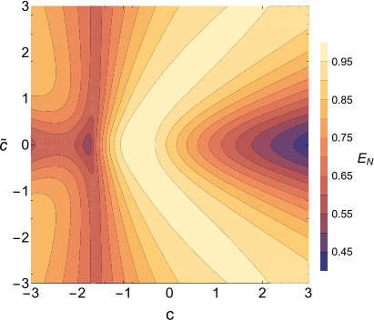
Figure 1: In this figure we present logarithmic negativity of the state (27), $E_{N}(\rho_{VV}(c,\tilde{c}))$ as a function of $c$, $\tilde{c}$. To obtain this plot we have inserted the measured values for the Higgs mass, Z mass and Z decay width, i.e., we put $\mathsf{b}_{Z}$, $\mathsf{e}_{Z}$, $\mathsf{f}_{Z}$, $\mathsf{h}_{Z}$ given in Eqs. (32,33,34,35).

IV Violation of Bell inequalities

Now, let us consider the violation of Bell inequalities in the state (27). The optimal Bell inequality for a two-qudit system was formulated in [48] and is known as the Collins–Gisin–Linden–Massar–Popescu (CGLMP) inequality. For two qubits ($d=2$) the CGLMP inequality reduces to the well known Clauser–Horn–Shimony–Holt (CHSH) inequality [49]. Here we are interested in the CGLMP inequality for a two-qutrit system (for spin-1 particle there are three possible outcomes of a spin projection measurements). In this case the CGLMP inequality has the following form

$$\mathcal{I}_{3}\leq 2,$$ (37)

where

$$\mathcal{I}_{3}=\big{[}P(A_{1}=B_{1})+P(B_{1}=A_{2}+1)\\ +P(A_{2}=B_{2})+P(B_{2}=A_{1})\big{]}\\ -\big{[}P(A_{1}=B_{1}-1)+P(B_{1}=A_{2})\\ +P(A_{2}=B_{2}-1)+P(B_{2}=A_{1}-1)\big{]}$$ (38)

and $A_{1}$, $A_{2}$ ($B_{1}$, $B_{2}$) are possible measurements that can be performed by Alice (Bob). Each of these measurements can have three outcomes: 0,1,2. Moreover, $P(A_{i}=B_{j}+k)$ denotes the probability that the outcomes $A_{i}$ and $B_{j}$ differ by $k$ modulo 3, i.e., $P(A_{i}=B_{j}+k)=\sum_{l=0}^{l=2}P(A_{i}=l,B_{j}=l+k\mod 3)$. As usual, we assume that Alice can perform measurements on one of the bosons, Bob on the second one, i.e., we take Alice (Bob) observables as $A\otimes I$ ($I\otimes B$).

To answer whether and how much a given quantum state $\rho$ violates the CGLMP inequality we have to find such observables $A_{1}$, $A_{2}$, $B_{1}$, $B_{2}$ for which the value of ${\mathcal{I}}_{3}$ is maximal in the state $\rho$ (so called optimal observables). But, in general, there does not exist a procedure of finding such optimal observables.

The CGLMP inequality (37) can be written as

$$\operatorname{Tr}\big{(}\rho\mathcal{O}_{\mathsf{Bell}}\big{)}\leq 2,$$ (39)

where $\mathcal{O}_{\mathsf{Bell}}$ is a certain operator depending on the observables $A_{1}$, $A_{2}$, $B_{1}$, and $B_{2}$.

Each Hermitian $3\times 3$ matrix $A$ can be represented with the help of the $3\times 3$ unitary matrix $U_{A}$, columns of $U_{A}$ are normalized eigenvectors of $A$ in a given basis. Using this notation in [12] it was shown that

$$\mathcal{O}_{\mathsf{Bell}}(U_{A_{1}},U_{A_{2}},U_{B_{1}},U_{B_{2}})=\\ -[U_{A_{1}}\otimes U_{B_{1}}]P_{1}[I\otimes S^{3}]P_{1}^{\dagger}[U_{A_{1}}\otimes U_{B_{1}}]^{\dagger}\\ +[U_{A_{1}}\otimes U_{B_{2}}]P_{0}[I\otimes S^{3}]P_{0}^{\dagger}[U_{A_{1}}\otimes U_{B_{2}}]^{\dagger}\\ +[U_{A_{2}}\otimes U_{B_{1}}]P_{1}[I\otimes S^{3}]P_{1}^{\dagger}[U_{A_{2}}\otimes U_{B_{1}}]^{\dagger}\\ -[U_{A_{2}}\otimes U_{B_{2}}]P_{1}[I\otimes S^{3}]P_{1}^{\dagger}[U_{A_{2}}\otimes U_{B_{2}}]^{\dagger},$$ (40)

where $S^{3}$ is the standard spin $z$ component matrix, $S^{3}=\mathrm{diag}(1,0,-1)$, and $P_{0}$, $P_{1}$ are $3^{2}\times 3^{2}$ block-diagonal permutation matrices:

$$P_{n}=\begin{pmatrix}C^{n}&\mathcal{O}&\mathcal{O}\\ \mathcal{O}&C^{n+1}&\mathcal{O}\\ \mathcal{O}&\mathcal{O}&C^{n+2}\end{pmatrix},\quad n=0,1,$$ (41)

where $\mathcal{O}$ is the $3\times 3$ null matrix and $C$ is the $3\times 3$ cyclic permutation matrix

$$C=\begin{pmatrix}0&0&1\\ 1&0&0\\ 0&1&0\end{pmatrix}.$$ (42)

Each $U$ from (40) can be taken as an element of $SU(3)$ group which has 8 parameters. Therefore, to perform the full optimization of $\mathcal{O}_{\mathsf{Bell}}$ for a given state one should optimize over the $32$ dimensional parameter space which is computationally challenging. Thus, usually, one applies a certain optimization procedure in order to find optimal observables.

In Appendix B of our previous paper [16] we described in detail two such procedures we used in the case $\tilde{c}=0$ (for the state of $Z$ bosons arising in the Higgs decay). The first of these procedures, originally introduced in [12], worked very well for $c$ close to 0. The second one, inspired by the proof of Theorem 2 in [50], allowed us to show that the CGLMP inequality is violated for all $c$. We will apply here this second procedure to show explicitly that CGLMP inequality is violated for all $c$, $\tilde{c}$ for all states (27) for which at least one off-diagonal element is non-zero (${\mathsf{f}}\not=0$ or ${\mathsf{h}}\not=0$). To this end, let us notice that the density matrix (27) can be written as

$$\rho_{VV}(c,\tilde{c})=\begin{pmatrix}0&0&0&0&0&0&0&0&0\\ 0&0&0&0&0&0&0&0&0\\ 0&0&\framebox{$a_{11}$}&0&\framebox{$a_{12}$}&0&\framebox{$a_{13}$}&0&0\\ 0&0&0&0&0&0&0&0&0\\ 0&0&\framebox{$a_{12}^{*}$}&0&\framebox{$a_{22}$}&0&\framebox{$a_{23}$}&0&0\\ 0&0&0&0&0&0&0&0&0\\ 0&0&\framebox{$a_{13}^{*}$}&0&\framebox{$a_{23}^{*}$}&0&\framebox{$a_{33}$}&0&0\\ 0&0&0&0&0&0&0&0&0\\ 0&0&0&0&0&0&0&0&0\end{pmatrix},$$ (43)

where $a_{11}+a_{22}+a_{33}=1$, $a_{11},a_{22},a_{33}\in{\mathbb{R}}_{+}$. Moreover, we define unitary matrices

$$U_{V}(t,\theta)=\begin{pmatrix}\cos\tfrac{t}{2}&0&e^{i\theta}\sin\tfrac{t}{2}\\ 0&1&0\\ -e^{-i\theta}\sin\tfrac{t}{2}&0&\cos\tfrac{t}{2}\end{pmatrix}$$ (44)

and

$$O_{A}=\begin{pmatrix}0&0&1\\ 0&-1&0\\ 1&0&0\end{pmatrix}.$$ (45)

Now, we calculate the mean value of the operator

$$(O_{A}\otimes I)\mathcal{O}_{\mathsf{Bell}}(U_{V}(0,0),U_{V}(\tfrac{\pi}{2},0),U_{V}(t,\theta),U_{V}(-t,\theta))\\ (O_{A}\otimes I)$$ (46)

in the state (43). The result can be written as

$${\mathcal{I}}_{3}=2+\tfrac{3}{2}\big{[}a(\cos{t}-1)-2|a_{13}|\cos(\alpha+\theta)\sin t\big{]},$$ (47)

where we used the following notation:

$$a_{11}+a_{33}=a,\qquad a_{13}=|a_{13}|e^{i\alpha},$$ (48)

and $a\geq 0$ as a sum of diagonal elements of a positive semidefinite matrix. The maximal value of (47) is attained for

$$\sin(\alpha+\theta)=0,\qquad\cos(\alpha+\theta)=\pm 1,$$ (49)

$$\cos t=\tfrac{a}{\sqrt{a^{2}+4|a_{13}|^{2}}},$$ (50)

$$\sin t=\mp\tfrac{2|a_{13}|}{\sqrt{a^{2}+4|a_{13}|^{2}}},$$ (51)

and is equal to

$$({\mathcal{I}}_{3})_{\mathrm{max}}=2+\tfrac{3}{2}\big{[}\sqrt{a^{2}+4|a_{13}|^{2}}-a\big{]}.$$ (52)

Thus, we see that $({\mathcal{I}}_{3})_{\mathrm{max}}>2$ for $|a_{13}|\not=0$.

To show that $({\mathcal{I}}_{3})_{\mathrm{max}}>2$ for $a_{12}\not=0$ or $a_{23}\not=0$ we need to change the block structure of the unitary matrices $U_{V}$ (44) putting a nontrivial $2\times 2$ block in the upper-left corner for $a_{12}\not=0$ or in the lower-right corner for $a_{23}\not=0$ (notice that in our case $a_{12}=a_{23}$). We do not present the detailed calculations here since they are similar to those given above.

Summarizing, we have shown that CGLMP inequality can be violated for all values of $c$, $\tilde{c}$ if at least one of the elements $a_{12}$, $a_{13}$, $a_{23}$ is non-zero.

It is very interesting that, as we have noticed in the Section III, the same condition holds for the state (27) to be entangled. In other words, we have shown that the state $\rho_{VV}(c,\tilde{c})$ (27) violates the CGLMP inequality iff it is entangled. It is a non-trivial observation since for an arbitrary $3\times 3$ quantum state $\rho$ such a statement is true only if $\rho$ is pure.

This also leads to strong phenomenological implications, since we have proven that in a pair of vector bosons one can indirectly test the violation of the Bell inequality by checking that the pair is entangled, which is a much easier experimental task. And this regardless of the interaction among the spin-0 particle and the gauge bosons (provided that they are CPT conserving and Lorentz invariant), so no future new physics can change the statement of entanglement and Bell violation in this system.

In our exemplary decay $H\to ZZ$ from Eqs. (32–35) we see that $a_{13}\not=0$. Therefore, in this decay the CGLMP inequality can be violated for all values of $c$, $\tilde{c}$. In Fig. 2 we have plotted the value of $({\mathcal{I}}_{3})_{\mathrm{max}}$ obtained with the help of the above optimization procedure for that decay.

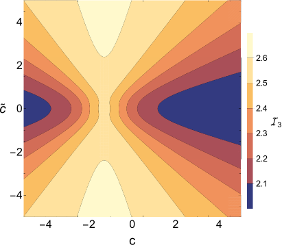
Figure 2: In this figure we present the maximal value of $\mathcal{I}_{3}$ in the state (27) as a function of $c$, $\tilde{c}$. We have inserted the measured values for the Higgs mass, Z mass and Z decay width, i.e., we put $\mathsf{b}_{Z}$, $\mathsf{e}_{Z}$, $\mathsf{f}_{Z}$ and $\mathsf{h}_{Z}$ given in Eqs. (32–35).

Comparing plots presented in Figs. 1 and 2 we see that state with the highest entanglement do not correspond to the state with the highest violation of the CGLMP inequality. This observation is consistent with the general property of CGLMP inequality [51].

Experimentally, the state $\rho_{ZZ}(c,\tilde{c})$ is reconstructed in collider experiments via quantum tomography methods [13, 52]. In such a case the presence of errors and background in the process $H\to ZZ\to f_{1}^{+}f_{1}^{-}f_{2}^{+}f_{2}^{-}$ modifies the state (27). To estimate how this modification influences the violation of the CGLMP inequality we consider the resistance of this violation with respect to the white noise. The noise resistance we define as a minimal value of $\lambda$, $\lambda_{\mathsf{min}}$, for which the state

$$\lambda\rho_{ZZ}(c,\tilde{c})+(1-\lambda)\tfrac{1}{9}I_{9},\qquad\lambda\in(0,1]$$ (53)

violates the CGLMP inequality. Inserting the state (53) into the CGLMP inequality (39) we obtain

$$\lambda_{\mathsf{min}}=\frac{2}{\max\{\operatorname{Tr}(\rho_{ZZ}(c,\tilde{c})\mathcal{O}_{\mathsf{Bell}})\}}.$$ (54)

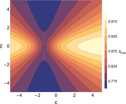
Figure 3: In this figure we present $\lambda_{\mathsf{min}}$ (54), as a function of $c$ and $\tilde{c}$. We have inserted the measured values for the Higgs mass, Z mass and Z decay width, i.e., we put $\mathsf{b}_{Z}$, $\mathsf{e}_{Z}$, $\mathsf{f}_{Z}$ and $\mathsf{h}_{Z}$ given in Eqs. (32–35).

We have plotted this value in Fig. 3 assuming that $\max\{\operatorname{Tr}(\rho_{ZZ}(c,\tilde{c})\mathcal{O}_{\mathsf{Bell}})\}$ is calculated with the help of the optimization procedure below Eq. (46). From this plot we can see that for values $c$, $\tilde{c}$ close to 0 we can tolerate up to almost a 20% of noise and still attain a violation of the CGLMP inequality and hence an entangled state.

As we mentioned before, there exist other optimization procedures then the one used in this paper. For example, one can focus on specific region of the $(c,\tilde{c})$ parameter space (e.g. close to $(0,0)$). Using such procedures one can attain larger violation of the CGLMP inequality in the considered region, which in consequence leads to higher noise tolerance.

Notice that values of $c$, $\tilde{c}$ close to 0 are expected for the decay $H\to ZZ$ due to experimental bounds on anomalous couplings for the $HZZ$ vertex [53]. We discuss these bounds in more details in B.

V Conclusions

We have discussed the CGLMP inequality violation and entanglement in a system of two vector bosons $V_{1}V_{2}$ produced in the decay of a pseudoscalar/scalar particle $X$. As an example of such a process we use the decay of the Higgs particle into two $Z$ bosons. We have assumed the most general CPT conserving, Lorentz-invariant coupling of the particle $X$ with the daughter bosons $V_{1}V_{2}$ (compare Eq. (2)). The amplitude of such a coupling depends on three parameters $v_{1}$, $v_{2}$, $v_{3}$. In the case of $H\to ZZ$, the Standard Model interaction corresponds to $v_{1}=1$, $v_{2}=v_{3}=0$. On the other hand $v_{3}\not=0$ implies the possibility of CP violation and a pseudoscalar component of $H$. Thus, we have assumed that $v_{1}\not=0$. In such a case, the state of produced bosons, beyond four-momenta and spins, can be characterized by two parameters $c$, $\tilde{c}$ which, up to normalization are equal to $v_{2}/v_{1}$ and $v_{3}/v_{1}$, respectively (cf. Eq. (7)). Next, in the center-of-mass frame, we have determined the most general pure state of $V_{1}V_{2}$ boson pair for a particular event $X\to V_{1}V_{2}$ and the $V_{1}V_{2}$ density matrix $\rho_{VV}(c,\tilde{c})$ obtained by averaging over kinematical configurations with an appropriate probability distribution (which can be obtained when both bosons subsequently decay into leptons). Finally, we have shown that this matrix is entangled and violates the CGLMP inequality for all values of $c$ and $\tilde{c}$ if at least one of off-diagonal elements of the density matrix is non-zero.

It is very interesting that, as we have shown, the state $\rho_{VV}(c,\tilde{c})$ (27) violates the CGLMP inequality iff it is entangled. It is a non-trivial observation since for an arbitrary $3\times 3$ quantum state $\rho$ such a statement is true only if $\rho$ is pure.

This also leads to strong phenomenological implications, since we have proven that in a pair of vector bosons one can indirectly test the Bell-type inequality violation by checking that the pair is entangled. And this is a much easier experimental task. Moreover, this observation holds regardless of the interaction among the spin-0 particle and the gauge bosons (provided that they are CPT conserving and Lorentz invariant, a very sensible requirement), so no future new physics can change the statement of entanglement and Bell violation in this system.

In the paper we have considered the case $v_{1}\not=0$ in order to compare the results with the actual decay $H\to ZZ$. However, even for $v_{1}=0$ we can use the same methods and obtain similar results. For instance, if $v_{3}=0$ as well then the state is always separable, while if $v_{3}\not=0$ one can define a single parameter, e.g. $(kp)v_{2}/v_{3}$, and perform an analogous analysis.

Appendix A Kinematics of the decay $X\to VV$ in the center of mass frame

We assume that the pseudoscalar/scalar particle $X$ in the CM frame has the four-momentum $(M,\textbf{0})$ and decays into two, possibly off-shell, $V$ bosons with four-momenta $k^{\mu}=(\omega_{1},\textbf{k})$, $\omega_{1}^{2}-\textbf{k}^{2}=m_{1}^{2}$ and $p^{\mu}=(\omega_{2},-\textbf{k})$, $\omega_{2}^{2}-\textbf{k}^{2}=m_{2}^{2}$. From energy conservation we get

$$M=\omega_{1}+\omega_{2},$$ (55)

and consequently, in the CM frame we have

$$\textbf{k}^{2} =\frac{1}{4M^{2}}\lambda(M^{2},m_{1}^{2},m_{2}^{2}),$$ (56)

$$kp =\frac{1}{2}\Big{[}M^{2}-m_{1}^{2}-m_{2}^{2}\Big{]},$$ (57)

$$\omega_{1} =\frac{1}{2M}\Big{[}M^{2}+(m_{1}^{2}-m_{2}^{2})\Big{]},$$ (58)

$$\omega_{2} =\frac{1}{2M}\Big{[}M^{2}-(m_{1}^{2}-m_{2}^{2})\Big{]},$$ (59)

where, following e.g. [20] we have defined the following function

$$\lambda(x,y,z)=x^{2}+y^{2}+z^{2}-2xy-2xz-2yz.$$ (60)

It is also convenient to introduce the following notation

$$\beta=\left.\tfrac{(kp)}{m_{1}m_{2}}\right|_{CM}=\frac{M^{2}-(m_{1}^{2}+m_{2}^{2})}{2m_{1}m_{2}}.$$ (61)

Appendix B Experimental and theoretical bounds on $c$, $\tilde{c}$ for the process $H\to ZZ$

For our exemplary decay $H\to ZZ$ there exist experimental and theoretical bounds on anomalous couplings $v_{2}$ and $v_{3}$ in the vertex (2). These bounds imply bounds on our parameters $c$, $\tilde{c}$. We discuss them briefly here.

Strong experimental bounds come from the measurements of Higgs boson particles performed at the LHC by the CMS Collaboration [22]. Comparing (2) in [22] and our Eq. (2) we obtain the following relation between the parameterizations used in our paper and in the CMS Collaboration paper:

$$v_{1} \propto a_{1}^{ZZ}m_{Z}^{2}+2a_{2}^{ZZ}(kp),$$ (62)

$$v_{2} \propto-2a_{2}^{ZZ},$$ (63)

$$v_{3} \propto a_{3}^{ZZ}$$ (64)

(with the same proportionality constant). In our previous paper [16] we have discussed the bounds on $c$, we obtained

$$|c|<c_{\mathsf{HZZ}}^{\mathsf{max}}=0.23.$$ (65)

Using similar argumentation for $\tilde{c}$ we obtain

$$|\tilde{c}|<\tilde{c}_{\mathsf{HZZ}}^{\mathsf{max}}=0.5.$$ (66)

From the theoretical point of view, perturbative unitarity (see, e.g., [54] for a recent review) can also constrain anomalous couplings. Using data from [55], we have shown in [16] that the requirement of perturbative unitarity does not limit accessible values of $c$ in the process $H\to ZZ$. We are not aware of any papers where perturbative unitarity is used to bound $v_{3}$.

References

- Bell [1964] J. S. Bell, On the Einstein Podolsky Rosen paradox, Physics Physique Fizika 1, 195 (1964).
- Freedman and Clauser [1972] S. J. Freedman and J. F. Clauser, Experimental test of local hidden-variable theories, Phys. Rev. Lett. 28, 938 (1972).
- Aspect et al. [1982] A. Aspect, J. Dalibard, and G. Roger, Experimental test of Bell’s inequalities using time-varying analyzers, Phys. Rev. Lett. 49, 1804 (1982).
- Rowe et al. [2001] M. A. Rowe, D. Kielpinski, V. Meyer, C. A. Sackett, W. M. Itano, C. Monroe, and D. J. Wineland, Experimental violation of a Bell’s inequality with efficient detection, Nature 409, 791 (2001).
- Ansmann et al. [2009] M. Ansmann, H. Wang, R. C. Bialczak, M. Hofheinz, E. Lucero, M. Neeley, et al., Violation of Bell’s inequality in Josephson phase qubits, Nature 461, 504 (2009).
- Pfaff et al. [2013] W. Pfaff, T. H. Taminiau, L. Robledo, H. Bernien, M. Markham, D. J. Twitchen, and R. Hanson, Demonstration of entanglement-by-measurement of solid-state qubits, Nature Physics 9, 29 (2013).
- Hensen et al. [2015] B. Hensen, H. Bernien, A. E. Dréau, A. Reiserer, N. Kalb, M. S. Blok, et al., Loophole-free Bell inequality violation using electron spins separated by 1.3 kilometres, Nature 526, 682 (2015).
- Giustina et al. [2015] M. Giustina, M. A. M. Versteegh, S. Wengerowsky, J. Handsteiner, A. Hochrainer, K. Phelan, et al., Significant-loophole-free test of Bell’s theorem with entangled photons, Phys. Rev. Lett. 115, 250401 (2015).
- Shalm et al. [2015] L. K. Shalm et al., Strong loophole-free test of local realism, Phys. Rev. Lett. 115, 250402 (2015).
- Barr [2022] A. J. Barr, Testing Bell inequalities in Higgs boson decays, Phys. Lett. B 825, 136866 (2022).
- Barr et al. [2023] A. Barr, P. Caban, and J. Rembieliński, Bell-type inequalities for systems of relativistic vector bosons, Quantum 7, 1070 (2023).
- Aguilar-Saavedra et al. [2023] J. A. Aguilar-Saavedra, A. Bernal, J. A. Casas, and J. M. Moreno, Testing entanglement and Bell inequalities in , Phys. Rev. D 107, 016012 (2023).
- Ashby-Pickering et al. [2023] R. Ashby-Pickering, A. J. Barr, and A. Wierzchucka, Quantum state tomography, entanglement detection and Bell violation prospects in weak decays of massive particles, J. High Energy Phys. 2023, 20 (2023).
- Aguilar-Saavedra [2023a] J. A. Aguilar-Saavedra, Laboratory-frame tests of quantum entanglement in , Phys. Rev. D 107, 076016 (2023a).
- Fabbrichesi et al. [2023a] M. Fabbrichesi, R. Floreanini, E. Gabrielli, and L. Marzola, Bell inequalities and quantum entanglement in weak gauge bosons production at the LHC and future colliders, Eur. Phys. J. C 83, 823 (2023a).
- Bernal et al. [2023] A. Bernal, P. Caban, and J. Rembieliński, Entanglement and Bell inequalities violation in with anomalous coupling, Eur. Phys. J. C 83, 1050 (2023).
- Fabbri et al. [2024] F. Fabbri, J. Howarth, and T. Maurin, Isolating semi-leptonic decays for Bell inequality tests, Eur. Phys. J. C 84, 20 (2024).
- Caban et al. [2008] P. Caban, J. Rembieliński, and M. Włodarczyk, Einstein-Podolsky-Rosen correlations of vector bosons, Phys. Rev. A 77, 012103 (2008).
- Caban [2008] P. Caban, Helicity correlations of vector bosons, Phys. Rev. A 77, 062101 (2008).
- Zagoskin and Korchin [2016] T. Zagoskin and A. Korchin, Decays of a neutral particle with zero spin and arbitrary CP parity into two off-mass-shell Z bosons, J. Exp. Theor. Phys. 122, 663 (2016).
- Godbole et al. [2007] R. M. Godbole, D. J. Miller, and M. M. Mühlleitner, Aspects of CP violation in the HZZ coupling at the LHC, J. High Energy Phys. 2007, 031 (2007).
- Sirunyan et al. [2019] A. M. Sirunyan et al. (CMS Collaboration), Measurements of the higgs boson width and anomalous couplings from on-shell and off-shell production in the four-lepton final state, Phys. Rev. D 99, 112003 (2019).
- Afik and de Nova [2021] Y. Afik and J. de Nova, Entanglement and quantum tomography with top quarks at the LHC, Euro. Phys. J. Plus 136, 907 (2021).
- Fabbrichesi et al. [2021] M. Fabbrichesi, R. Floreanini, and G. Panizzo, Testing Bell inequalities at the lhc with top-quark pairs, Phys. Rev. Lett. 127, 161801 (2021).
- Aguilar-Saavedra and Casa [2022] J. A. Aguilar-Saavedra and J. A. Casa, Improved tests of entanglement and Bell inequalities with LHC tops, Eur. Phys. J. C 82, 666 (2022).
- Aoude et al. [2022] R. Aoude, E. Madge, F. Maltoni, and L. Mantani, Quantum SMEFT tomography: Top quark pair production at the LHC, Phys. Rev. D 106, 055007 (2022).
- Dong et al. [2023] Z. Dong, D. Gonçalves, K. Kong, and A. Navarro, When the machine chimes the Bell: Entanglement and Bell inequalities with boosted (2023), arXiv: 2305.07075 [hep-ph], arXiv:2305.07075 [hep-ph] .
- Severi et al. [2022] C. Severi, C. Boschi, F. Maltoni, and M. Sioli, Quantum tops at the lhc: from entanglement to bell inequalities, Eur. Phys. J. C 82, 285 (2022).
- Afik and de Nova [2023] Y. Afik and J. de Nova, Quantum discord and steering in top quarks at the LHC, Phys. Rev. Lett. 130, 221801 (2023).
- Severi and Vryonidou [2023] C. Severi and E. Vryonidou, Quantum entanglement and top spin correlations in SMEFT at higher orders, J. High Energ. Phys. 2023, 148.
- Aad et al. [2023] G. Aad et al. (ATLAS Collaboration), Observation of quantum entanglement in top-quark pairs using the ATLAS detector (2023), arXiv: 2311.07288 [hep-ex], arXiv:2311.07288 [hep-ex] .
- CMS Collaboration [2024] CMS Collaboration, CERN report CMS-PAS-TOP-23-001 (2024).
- Morales [2023] R. A. Morales, Exploring Bell inequalities and quantum entanglement in vector boson scattering, Eur. Phys. J. Plus 138, 1157 (2023).
- Sinha and Zahed [2023] A. Sinha and A. Zahed, Bell inequalities in 2-2 scattering, Phys. Rev. D 108, 025015 (2023).
- Takubo et al. [2021] Y. Takubo, T. Ichikawa, S. Higashino, Y. Mori, K. Nagano, and I. Tsutsui, Feasibility of bell inequality violation at the atlas experiment with flavor entanglement of pairs from collisions, Phys. Rev. D 104, 056004 (2021).
- Aguilar-Saavedra [2023b] J. A. Aguilar-Saavedra, Postdecay quantum entanglement in top pair production, Phys. Rev. D 108, 076025 (2023b), 2307.06991 .
- Bi et al. [2024] Q. Bi, Q.-H. Cao, K. Cheng, and H. Zhang, New observables for testing Bell inequalities in boson pair production, Phys. Rev. D 109, 036022 (2024).
- Ehatäht et al. [2024] K. Ehatäht, M. Fabbrichesi, L. Marzola, and C. Veelken, Probing entanglement and testing bell inequality violation with at belle ii, Phys. Rev. D 109, 032005 (2024).
- Sakurai and Spannowsky [2024] K. Sakurai and M. Spannowsky, Three-body entanglement in particle decays, Phys. Rev. Lett. 132, 151602 (2024).
- Aguilar-Saavedra [2024] J. A. Aguilar-Saavedra, Tripartite entanglement in decays (2024), arXiv: 2403.13942 [hep-ph], arXiv:2403.13942 [hep-ph] .
- Maltoni et al. [2024] F. Maltoni, C. Severi, S. Tentori, and E. Vryonidou, Quantum detection of new physics in top-quark pair production at the LHC, J. High Energ. Phys. 2024, 99.
- Aoude et al. [2023] R. Aoude, E. Madge, F. Maltoni, and L. Mantani, Probing new physics through entanglement in diboson production, J. High Energ. Phys. 2024, 17.
- Fabbrichesi et al. [2023b] M. Fabbrichesi, R. Floreanini, E. Gabrielli, and L. Marzola, Stringent bounds on and anomalous couplings with quantum tomography at the LHC, Eur. Phys. J. C 2023, 195 (2023b).
- Barr et al. [2024] A. J. Barr, M. Fabbrichesi, R. Floreanini, E. Gabrielli, and L. Marzola, Quantum entanglement and Bell inequality violation at colliders (2024), arXiv:2402.07972 [hep-ph], arXiv:2402.07972 [hep-ph] .
- Workman et al. [2022] R. L. Workman et al. (Particle Data Group), Review of Particle Physics, PTEP 2022, 083C01 (2022).
- Vidal and Werner [2002] G. Vidal and R. F. Werner, Computable measure of entanglement, Phys. Rev. A 65, 032314 (2002).
- Plenio [2005] M. B. Plenio, Logarithmic negativity: A full entanglement monotone that is not convex, Phys. Rev. Lett. 95, 090503 (2005).
- Collins et al. [2002] D. Collins, N. Gisin, N. Linden, S. Massar, and S. Popescu, Bell inequalities for arbitrarily high-dimensional systems, Phys. Rev. Lett. 88, 040404 (2002).
- Clauser et al. [1969] J. F. Clauser, M. A. Horne, A. Shimony, and R. A. Holt, Proposed experiment to test local hidden-variable theories, Phys. Rev. Lett. 23, 880 (1969).
- Popescu and Rohrlich [1992] S. Popescu and D. Rohrlich, Generic quantum nonlocality, Phys. Lett. A 166, 293 (1992).
- Acín et al. [2002] A. Acín, T. Durt, N. Gisin, and J. I. Latorre, Quantum nonlocality in two three-level systems, Phys. Rev. A 65, 052325 (2002).
- Bernal [2023] A. Bernal, Quantum tomography of helicity states for general scattering processes (2023), arXiv: 2310.10838 [hep-ph], arXiv:2310.10838 [hep-ph] .
- Rao et al. [2021] K. Rao, S. D. Rindani, and P. Sarmah, Study of anomalous gauge-Higgs couplings using Z boson polarization at LHC, Nucl. Phys. B 964, 115317 (2021).
- Logan [2022] H. E. Logan, Lectures on perturbative unitarity and decoupling in Higgs physics (2022), arXiv:2207.01064 [hep-ph], arXiv:2207.01064 [hep-ph] .
- Dahiya et al. [2016] M. Dahiya, S. Dutta, and R. Islam, Investigating perturbative unitarity in the presence of anomalous couplings, Phys. Rev. D 93, 055013 (2016).