Thousand foci coherent anti-Stokes Raman scattering microscopy
Abstract
We demonstrate coherent anti-Stokes Raman scattering (CARS) microscopy with 1089 foci, enabled by a high repetition rate amplified oscillator and optical parametric amplifier. We employ a camera as multichannel detector to acquire and separate the signals from the foci, rather than using the camera image itself. This allows to retain the insensitivity of the imaging to sample scattering afforded by the non-linear excitation point-spread function, which is the hallmark of point-scanning techniques. We show frame rates of 0.3 Hz for a megapixel CARS image, limited by the camera used. The laser source and corresponding CARS signal allows for at least 1000 times higher speed, and using faster cameras would allow acquiring at that speed, opening a perspective to megapixel CARS imaging with more than 100 Hz frame rate.
I Introduction
Coherent Raman scattering (CRS) allows microscopy with chemical selectivity using the vibrational response of the chemical components of the sample without adding fluorescent dyes.[1, 2, 3, 4] Driving the vibrations by an optical excitation which is intensity modulated at the vibrational frequency, the vibrations are in turn modulating the polarisability, creating coherent side-bands of the optical excitation fields. These sidebands are the CRS, and their amplitude and phase encode the vibrational spectrum of the medium probed. Since its revival about 2 decades ago[5] enabled by the development of suited commercial laser sources, the field has developed a wide range of methods of excitation and detection, with different advantages and drawbacks. [1, 4]
The most common scheme uses two synchronised optical pulses, the pump pulse and the longer wavelength Stokes pulse, with a frequency difference given by the vibrational frequency of interest. To achieve high intensities while keeping the average power below sample damage, pulses of picosecond duration, comparable to the typical vibrational coherence times in condensed matter, with repetition rates in the 1-100 MHz range are employed, having a duty cycle in the to range. Focussing these pulses to the diffraction limit of high numerical aperture (NA) objectives of about 0.5 µm size enables achieving peak intensities of the order of W/cm2 for average powers of tens of milliwatts, suitable for efficient CRS generation just below typical saturation levels[6] around W/cm2. Scanning this focus across the sample is then used to provide an image, similar to other multiphoton techniques recording two-photon fluorescence (TPF), second harmonic generation (SHG), or third harmonic generation (THG). The non-linearity of the CRS signal with the excitation intensity enables optical sectioning without imaging in the detection, an advantage compared to confocal or other structured illumination microscopes, specifically for inhomogeneous samples exhibiting significant diffuse scattering.
The high frequency sideband of the pump, called coherent anti-Stokes Raman scattering (CARS), and the low frequency sideband of the Stokes, call coherent Stokes Raman scattering (CSRS), can be detected free of excitation background, while the high frequency sideband of the Stokes interferes with the pump, called stimulated Raman loss (SRL), and the low frequency sideband of the pump interferes with the Stokes, and is called stimulated Raman gain (SRG). Notably, sidebands are also created by purely electronic non-linearities such as the Kerr effect, as well as by vibrational resonances at higher frequencies, providing a background to the resonant response. These non-resonant responses are in quadrature to the pump or Stokes beams in SRL and SRG, respectively, yielding in lowest order only a change of phase without changing the amplitude. Thus by detecting the transmitted power, which is insensitive to the phase, only resonant responses are measured, rendering SRL and SRG spectra similar to Raman spectra. However, the relative changes are typically very small, in the to range, so that high-frequency modulation schemes and shot-noise limited laser sources are required.
Detecting the CARS or CSRS power, free of excitation background, does not have these requirements, but the signal contains the interference between resonant and non-resonant response, creating asymmetric resonance lineshapes, complicating the interpretation of the contrast. To retrieve a signal linear in the concentration of the chemical components, the complex susceptibility can be determined by phase retrieval using the causality of the response and the measured dependence on the vibrational frequency.[7, 8, 9]
The point scanning approach has been optimised and is now limited by the maximum signal available due to signal saturation by excitation of higher vibrational levels [6] or heating, and allows for video rate imaging.[10, 11, 12] However, small absorbing regions can lead to sample damage at the high intensities and repetition rates used, both by heating and by avalanche breakdown. Recently there was some effort to use squeezed light [13] to reduce the shot-noise in SRL and SRG, with modest success (less than a factor of two in signal to noise) limited by the un-squeezing of the detected light by losses due to scattering in the sample and finite transmission of optical elements. Thus the only clear way forward to higher speed is to distribute the excitation into many focal spots, or use a wide-field illumination. This requires suited laser sources providing the larger pulse energy required to provide an intensity sufficiently high for efficient CRS generation across the extended excitation region. To limit the average power on the sample, the repetition rate of the laser pulses need to be reduced, which also allows the laser-induced heating and electronic excitations to dissipate between pulses, increasing damage thresholds.
Early wide-field approaches used nanosecond pulsed lasers with repetition rates in the 1-100 Hz range and a non-colinear geometry for phase matching, enabling to choose between dark-field (phase-mismatched) and bright-field (phase-matched) imaging.[14] The method was applied to image 2D cell cultures,[15] but the coherent wide-field nature of the signal created significant interference artefacts, specifically relevant for thicker and more scattering samples, and furthermore did not provide sectioning. This drawback was addressed using random speckle illumination, which after speckle averaging resembles a spatially incoherent illumination and thus removes the interference artefacts.[16] Multimode optical fibres were used to generate the speckles, with the Stokes beam of a coherence length much larger than the phase delay distribution across the fibre modes retaining the spatial speckle pattern, while the pump beam of a shorter coherence length creating a spatio-temporal speckle pattern which provides some speckle averaging already over a single pulse.[16] Furthermore, using a varying speckle pattern across many camera frames, and evaluating the fluctuations, the sectioning capability was recovered, but with a random noise in the image scaling with the inverse root of the number of independent frames, a number limited by signal strength and camera technology. Notably, the image formation relies exclusively on the imaging of the signal onto the camera, and is thus affected by scattering of the sample in the collection path. The absence of a suited technical solution measuring the weak SRL or SRG modulation with an imaging detector presently limits these widefield techniques to CARS and CSRS.
Recently, the wide-field speckle CARS imaging concept was revisited,[17] using an optical parametric amplifier providing a much higher repetition rate (515 kHz). The Stokes speckle pattern was changed only between camera frames, while the pump speckle pattern was changed many times over a single camera frame to provide averaging. A reconstruction algorithm (Wiener filtering) was used to increase the spatial resolution of the retrieved speckle fluctuation image in-plane. Notably, the issue of the speckle noise requiring averging over many frames and the reliance on imaging in the collection path remained.
Instead of wide-field illumination, increasing the number of foci for fast scanning is a known concept in confocal microscopy[18] (Nipkow disk scanners), and also in multiphoton microcopy [19, 20] where camera imaging in the detection path was used to provide the lateral resolution. Sectioning is created by apertures in the detection imaging for confocal microscopy and by the focussed excitation itself in multiphoton microscopy. The inherent trade-off between the number of foci used and the sectioning capability has been investigated.[21] The only multifocal CARS imaging reported[22] up top now employed two synchronised Ti:Sapphire oscillators delivering 5 ps pulses at 80 MHz repetition rate. A rotating microlens array created an average of seven focal spots moving across the sample at any given time, and CARS was imaged onto a camera, which during the exposure time averaged the signal over the microlens positions fully covering the imaged area. Due to the low pulse energy available, the number of foci and the speed was rather limited, and while an application to cell imaging was shown, [23] the method was not pursued further.
In the present work, we revisit the multi-focal CARS microscopy concept, and demonstrate imaging with a much larger number of 1089 foci at high speed. Importantly we introduce the use of a camera as a multi-segment detector to suppress the detrimental influence of scattering in the detection imaging. The commercial availability of high pulse energy and high repetition rate laser systems such as employed in Ref. 17 enables the excitation of a large number of foci without compromising on the CARS efficiency. Furthermore, the availability of fast and low noise CMOS cameras allows read out of the CARS image for every position of the foci. This enables to use the camera images to determine the signal created by each individual focus by summing over a defined region for each focus, emulating the non-imaging single channel detectors employed in single point scanning techniques. The spatial resolution of the resulting CARS image is created by the multiphoton excitation process, as in single point scanning techniques, allowing for deeper penetration into scattering samples.
II Methods
II.1 Samples
Sample O providing a homogeneous reference was prepared by pipetting 10 µL of olive oil (Bio Basso by Basso Fedele & Figli srl) onto a glass coverslip (#1.5, mm2, Thermo Scientific) and was spread across by adding a second equal coverslip for imaging.
Sample A providing bead arrays in water was prepared by pipetting 10 µL of 1% solid suspension PS beads of 2 µm diameter (124, Phosphorex) onto a glass coverslip (#1.5, mm2, Thermo Scientific). The mixture was left to dry at ambient conditions and 10 µL of distilled water was pipetted onto the coverslip and spread across the sample by adding a second equal coverslip for imaging.
Sample B providing a bead mixture in oil was prepared by mixing 10 µL of 1% solid suspension of polymethyl methacrylate (PMMA) beads of 20 µm diameter (MMA20K, Phosphorex) and 10 µL of 1% solid suspension polystyrene (PS) beads of 10 µm diameter (118, Phosphorex) on a glass coverslip as above. The mixture was left to dry under ambient conditions for 30 mins. Subsequently, 10 µL of olive oil was pipetted onto the coverslip and spread across the sample by adding a second equal coverslip for imaging.
Sample C providing small beads to demonstrate the point spread function (PSF) was prepared by pipetting 10 µL of 1% solid suspension PS beads of 0.5 µm diameter (108, Phosphorex) onto a coverslip as above and dried at ambient conditions.
Human skin sarcoma samples to demonstrate imaging performance were prepared by fixing them with 10% formalin and dehydrating it with ethanol. The embedding was performed by using paraffin and the sample was sectioned with a microtome. The sample was stained by using a standard eaosin and hematoxylin staining procedure.[24]
II.2 Experimental Setup
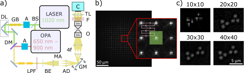
The experimental setup used is sketched in Fig. 1a. An amplified laser system (PHAROS, Light Conversion) provides transform-limited 290 fs pulses of 1020 nm center wavelength at 200 kHz repetition rate and 20 W average power. 5 W of the beam are used as Stokes beam for CARS, while the remaining power is used for an optical parametric amplifier (OPA) (ORPHEUS-F, Light Conversion) which provides 130 fs pulses tunable from 650 to 900 nm with 1 W average power, used as pump beam for CARS. The powers of pump and Stokes are controlled by attenuators consisting of a half-wave plate (Castech) and a Glan-Taylor polarizer (GT10-B, Thorlabs). The Stokes beam is transmitted through 60 mm of SF-66 glass blocks (II-VI incorporated) and an optical delay line (VT-80, PI) with silver retroreflectors (Eksma optics) to control the temporal overlap of pump and Stokes at the sample. Both beams are combined into the same spatial mode by a dichroic mirror (high reflection from 600 to 950 nm and high transmission from 970 to 1300 nm, Eksma Optics) and then pass through 145 mm of SF-57 glass blocks (II-VI incorporated) for spectral focussing.[25, 26] The pump at 785 nm accrues 33350 of group delay dispersion (GDD) stretching it to 723 fs, while the fixed Stokes accrues 34450 GDD stretching it to 439 fs. The difference in GDD can be compensated using a commercially available pulse compressor (Light Conversion) which can add up to 1300 GDD to the pump beam. Both beams then pass through a long-pass filter (FEL0700, Thorlabs) to remove components below 700 nm wavelength, spectrally overlapping with the CARS signal (mostly residuals of the white-light generation seed of the OPA). A beam expander (plano-concave lens of focal length mm and plano-convex lens of mm, Casix) increases the beam size from 3 mm to 9 mm. The beams then are focussed by a silica microlens square array (15-811, Edmund Optics) of mm2 size, 300 µm pitch, and mm, creating focal spots. The generated beamlets are collimated by an achromatic doublet (PO-PK-L3, II-VI incorporated) of mm, and are merging at its back-focal plane which is located at the x-y galvo mirrors (6215H, Cambridge Technology) scanning the beam directions. The beamlets are then relayed with four-times magnification (closely-spaced pair of AC300-100-B and a AC508-200-B-ML, Thorlabs), expanding the beamlets to mm2 square size and imaging the galvo mirrors into the 15 mm diameter back focal plane of the excitation objective (plan apo lambda 20 0.75 NA, MRD00205, Nikon), which focuses the beamlets into the sample. The transmitted light is collected by a second objective (plan apo VC 20 0.75 NA, 1501-9398, Nikon) and then passes through a short-pass and a band-pass optical filter (FESH0750 and FB650-40, Thorlabs) to isolate the CARS signal. A camera lens of mm and /2.8 aperture (NMV-50M23, Navitar) images the sample with a magnification of 5 onto a camera of pixels of 3.45 µm size, e read noise, 10 ke full well capacity, and USB3.1 interface (BFS-U3-51S5M-C, FLIR). The 18 mm aperture of the camera objective accommodates the 15 mm diameter of the collection objective back focal plane and allows for some off-axis beam walk-off. We note that the 5 times magnification onto the camera is slightly below the 7 times required for Nyquist sampling, which reduces the number of pixels to be read per focal spot, improving read noise and speed. The camera is triggered via the software driving the galvos with a frame rate , and the exposure time is set to allow this frame rate, which requires with the delay time µs. The camera is read with 8bit pixel format for highest speed, via a software written in LabView, and the frames are saved as bitmaps and processed off-line. We note that real-time processing of the data would be feasible with more software development. We used a camera analog gain of 10dB, 20dB or 30dB, providing 14.6, 4.61, or 1.46 e/count, respectively, and a digital offset of 5 counts to avoid zero-clipping. The dark signal was subtracted from each frame before further processing. Powers of excitation beams given later are measured at the sample.
II.3 Image acquisition
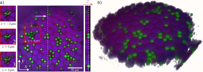
The CARS signal generated in the sample is imaged onto the camera, showing the grid of beamlet foci, as seen in Fig. 1b for the homogeneous sample O. The intensities of the foci are varying across the array due to the variation of the beam intensity across the lenslet array considering the pump and Stokes excitation beams of Gaussian beam diameter (at intensity) of 9 mm, resulting in a gradual reduction towards the periphery of the array. Notably, CARS is a third-order signal proportional to , with the pump intensity and the Stokes intensity , resulting in a diameter of the CARS intensity of about 5 mm, a factor of smaller than the beams.
The galvo-mirrors are used to shift the foci in a raster-scan pattern with steps in each direction, filling the space between foci, as sketched in Fig. 1b. We note that this could also be achieved by simply laterally shifting the microlens array. An image is acquired at each rasterscan index in and direction for . The foci are separated by 7.5 µm on the sample, which corresponds to pixels on the camera. The focal point positions of the beamlets of index in and directions, , are determined using the signal peak positions in the image from the homogeneous sample. The camera centering and rotation is aligned so that the central row and column of foci are straight and deviating by less than half a pixel from the horizontal and vertical direction. A second-order polynomial is then fitted to the horizontal positions of the central row of peaks (), and equivalently to the vertical positions of the central column of peaks (), and the position of any peak is then taken as for image reconstruction. The second-order terms cater for small cushion distortions of the imaging. The nominal focus positions in are then taken as and are providing the signal for the pixel position in the excitation image, having a pixel size on the sample of 7.5 µm/.
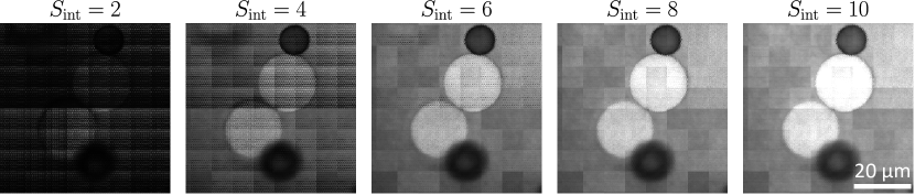
The pixel value of the excitation image is evaluated by summing the pixel values of over a square area with edge size centred on the nominal focus positions (see green area in Fig. 1b), noting that avoiding overlap between foci requires . The number of pixels summed is , providing a read noise of , proportional to . The variation of with depends on the extension of the imaged signal in . In homogeneous samples the extension is below 2 pixels, as seen in Fig. 1b, thus choosing seems appropriate to achieve highest signal to noise. However, the extension is affected by sample inhomogeneities in the path from the beamlet focus to the camera, as exemplified in Fig. 9. Thus the immunity of against sample inhomogeneities increases with , and is maximised for , as shown in Fig. 7. Excitation images of 2 µm PS beads (sample A) at 2950 are given in Fig. 1c using different , showing the increasing definition of the imaged beads with . Nyquist sampling is achieved for , providing a pixel size of 250 nm.
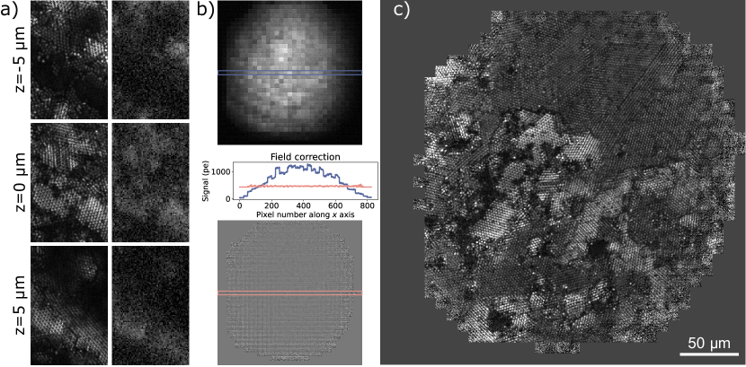
The use of the camera to define a multi-segment detector separating the signal of each focus in the excitation imaging can be compared with the detection imaging employed in previous multifocal approaches,[19, 22] where the image is given by the sum of over all . The resulting detection imaging is shown in Fig. 2a for sample A in a region with stacked patches of closely packed 2 µm PS beads in water, imaged at different axial planes. A significant blurring and reduced contrast in detection imaging (right column) compared to excitation imaging (left column) is observed. We note that the detection imaging pixel size of 0.69 µm is sufficient to resolve the beads. Thus, while the excitation imaging results in a PSF given by the excitation focus as in single point scanning, detection imaging results in blurring due to sample inhomogeneities, an issue intrinsic to the previous multifocal approaches.
II.4 Image post-processing
Variations between microlenses lead to variations in the CARS signal from different foci. Moreover, these differences are modulated by sample inhomogeneities. Static, sample independent variations can be corrected using an image of a homogeneous sample and calculating the ratio of the average pixel value over the tile from an individual focus to the average value of all tiles . To exclude tiles of low signal, exhibiting excessive noise after correction, tiles with a ratio lower than a threshold value are set to the average value of the other tiles . The flat-field corrected pixel values are accordingly calculated as
| (1) |
The uncorrected pixel values for the homogeneous sample O are presented in Fig. 2b. A tile structure from imperfections in the microlens array, and vignetting by the finite excitation beam size are visible. Applying the flat-field correction Eq. 1, the resulting image is rather uniform (see Fig. 2b bottom and red cross-section). There is a remaining gradient of some % across the tiles, which is attributed to clipping of the excitation beams and the CARS signal by the objectives and could be reduced optimising the optical layout.
A corrected image of sample A with 2 µm PS beads is presented in Fig. 2c, showing the high imaging quality achieved. Notably, even after correction, a tiling pattern is still visible. We attribute this to a distortion of the individual foci by the sample, which can reduce or increase the CARS signal depending on the distortions present without the sample due to the imperfection of the microlens array. Therefore the relative intensity of the foci does depend on the refractive index inhomogeneities of the sample itself, and cannot be fully compensated by a reference measurement on a homogeneous sample. These effects could be mitigated using a higher quality microlens array.
As alternative to hardware improvements, we developed an algorithm to minimise the tile pattern a posteriori. This algorithm determines correction factors for each beamlet to minimise the step heights at the tile edges over all tiles. To do so, we determine the edge ratios of a tile ,
| (2) |
for the right edge, and
| (3) |
for the bottom edge. These edge ratios are modified by applying the tiling correction factors , and we find the factors minimising the deviation of the modified ratios from unity using
The tiling corrected data is then given by . An example of the tiling correction is discussed later in Fig. 5.
III Results
III.1 Point spread function
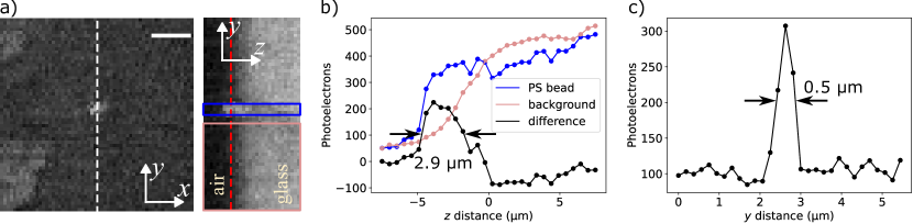
To measure the experimental three-dimensional PSF of the setup, a 0.5 µm diameter PS bead on glass in air (sample C) was imaged. Flat-field corrected images in the x-y as well as y-z planes are presented in Fig. 3. The in-plane PSF full width at half maximum (FWHM) is 0.5 µm, while the axial PSF FWHM is 2.9 µm, comparable to previous single point scanning data using an 0.75 NA objective.[27]
III.2 Tiling correction
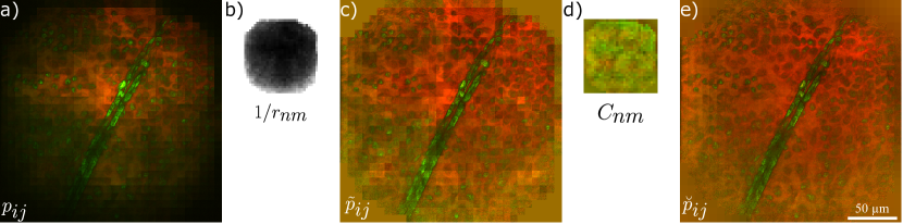
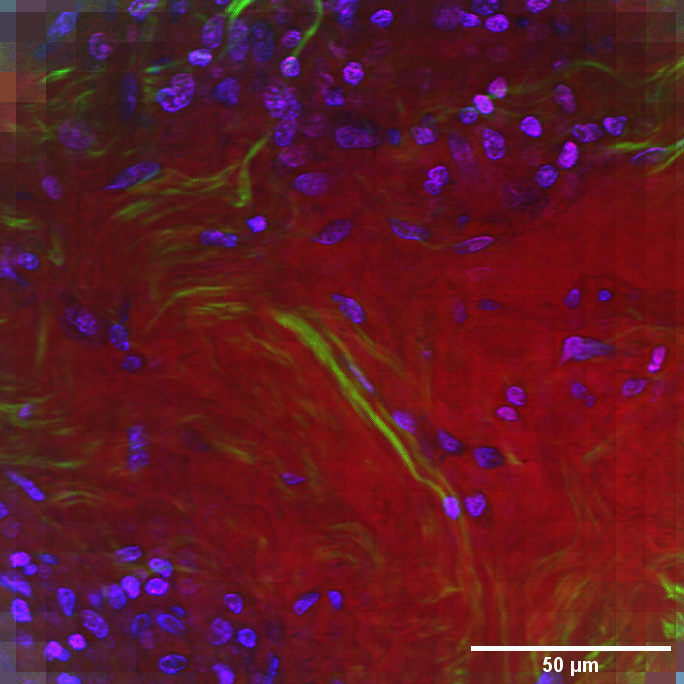
To demonstrate the efficacy of the tiling correction on biomedical samples of interest, a human skin sample (see Sec. II.1) was imaged at 2935 and 2970 . The resulting data using is presented in Fig. 4a. The vignetting due to the excitation beam profiles is clearly visible, together with the tiling. After flat-field correction using from sample O and (see Fig. 2), shown in Fig. 4b, the resulting given in Fig. 4c shows that the vignetting has been corrected, but the tiling, while somewhat reduced, is still clearly visible. The change in the tile pattern indicates that the origin of the remaining pattern is different from the tiling in a homogeneous medium. Applying the tiling correction Eq. II.4 yields the factors shown in Fig. 4d. The corrected given in Fig. 4e is void of significant tiling, confirming that the correction is effective. The visible structure is attributed to basal cells (circular objects) in a collagen matrix and elastin (tubular shape).
III.3 Three-dimensional bead imaging
To demonstrate the z-sectioning capability on strongly scattering structures, sample B hosting a mixture of 20 µm PMMA beads and 10 µm PS beads in oil was imaged. A -stack over 10 positions with 2 µm increments was measured. Using different pump-Stokes delays, CARS stacks at 2930 dominated by oil, at 2950 dominated by PMMA, and at 3050 dominated by PS were sequentially recorded. Flat-field and tiling correction was applied, and the resulting is shown in Fig. 5. We can see that the method is able to create well resolved -sectioning also for strongly scattering samples. Comparing this with detection imaging as previously used[19, 22] and shown in Fig. 8, the significant advantage of excitation imaging created by the non-linear exitation PSF is evident. Nevertheless, the 10 µm PS beads with their large refractive index contrast to olive oil (1.59 to 1.46) provide such large deviations in the detection imaging that the signals from different foci are mixed, as detailed in Fig. 9. This mixing leads to the shadowing of the lower PS beads by the beads lying on top of them in Fig. 5a 1-3. Considering that the shadowing shows the obstacles in detection direction, increasing the NA of excitation and detection would spatially blur and thus reduce the shadowing.
III.4 CARS and SHG imaging of human skin
To demonstrate the performance of the multifocal approach on medically relevant scattering samples, a human skin tissue was imaged (see Sec. II.1). CARS was recorded at 2935 and 2970 . To measure SHG of the Stokes, the FB650-40 filter was replaced by a BP520-40 (Thorlabs), and the pump was blocked. The glass blocks were not removed for convenience, but we note that the SHG signal would be increased about 4 times by doing so. The resulting image encoding all three data as false colour is presented in Fig. 6. We attribute the structure to basal cells (blue), elastin fibres (green), and collagen matrix (red).
IV Conclusions
In this work we have demonstrated multifocal CARS microscopy with 1089 foci, enabled by a high repetition rate amplified oscillator and optical parametric amplifier. Importantly, different from previous multifocal approaches,[19, 22] we introduced employing the camera detection only to separate the signals of the different foci, and not for imaging. This retains the insensitivity to sample scattering afforded by the non-linear excitation PSF created by longer wavelength light, which is the hallmark of point-scanning CRS. Notably, speckle widefield CARS[16, 17] is using detection imaging and also has intrinsic speckle noise.
The speed of the technique in the present setup is limited by the camera readout, while the laser source caters for up to ten times higher excitation powers, and correspondingly 1000 times higher CARS powers, allowing to increase the speed accordingly, up to frames per second. This would enable a 100 Hz frame rate for megapixel CARS images, corresponding to 10 ns pixel rate, about an order of magnitude faster than the fastest single point scanning systems. Notably, due to the 1000 foci, this is achievable with similar single focus power densities using a 100 times lower repetition rate than single point systems. Since the camera is only used to separate the different foci rather than to image the sample at the Nyquist limit, only a small number of pixels are required, for example pixels would suffice for 1000 foci, which can be read by present camera technology at up to frames per second, opening the perspective to megapixel CARS imaging with 1000 Hz frame rates.
As future improvement of the method, time-multiplexing[28] is a promising approach not only for suppression of cross-talk between foci as demonstrated for TPF,[28] but also to address different vibrational frequencies via spectral focussing, allowing for a spectrally resolved imaging where different foci address different vibrational resonances, doing away with the sequential spectral tuning.
Acknowledgements.
We wish to acknowledge Jonas Berzinš (Light Conversion) for proofreading and commenting on the draft, Skaidra Valiukevičienė (Lithuanian University of Health Sciences) for human skin sarcoma samples, and Paola Borri for support. This project has received funding from the European Union’s Horizon 2020 research and innovation programme under the Marie Skłodowska-Curie grant agreement No 812992.Appendix A Influence of detection region size on excitation image
The size of the region used to sum the signal for each excitation focus is determining the properties of the resulting exictation image , as discussed in Sec. II.3. This dependence is exemplified in Fig. 7, showing for detection region sizes from 2 to 10 for PS and PMMA beads embeded in oil. One finds that for small , for which the detection region does not fully cover the signal from each focus, stripes appear due to the discrete positioning governed by the pixelation of . With increasing , the fraction of the collected signal increases and saturates, providing an image free of the pixelation artifact, only carrying the tile pattern from the variation between foci.
Appendix B Detection and excitation imaging of beads
Fig. 8 shows a comparison between detection imaging and excitation imaging for the bead sample B. The detection image is of lower sharpness and contrast compared to the excitation image . Notably since , there are 900 pixels per focus in , while there are camera pixels over the same area, resulting in a higher signal per pixel in .
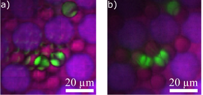
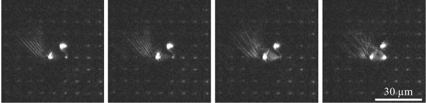
The beads in sample B can lead to a strong scattering of the CARS signal in detection imaging, due to the high index contrast beween PS and oil. This is exemplified in selected frames shown in Fig. 9, and in the movie of all frames provided in the file Scattering.avi. The beads can form whispering gallery modes by total internal reflection, leading to the observed standing wave patterns. Notably, the signal is distributed widely across the frame, well beyond the detection region size , resulting in cross-talk between foci creating weak ”phantom” images of the PS beads, and inhomogeneous signal within the PS beads, visible in Fig. 8a.
References
- Zumbusch, Langbein, and Borri [2013] A. Zumbusch, W. Langbein, and P. Borri, “Nonlinear vibrational microscopy applied to lipid biology,” Progress in Lipid Research 52, 615–632 (2013).
- Zhang, Zhang, and Cheng [2015] C. Zhang, D. Zhang, and J.-X. Cheng, “Coherent Raman Scattering Microscopy in Biology and Medicine,” Annu. Rev. Biomed. Eng. 17, 415–445 (2015).
- Zhang and Aldana-Mendoza [2021] C. Zhang and J. A. Aldana-Mendoza, “Coherent Raman scattering microscopy for chemical imaging of biological systems,” Journal of Physics: Photonics 3, 032002 (2021).
- Lin and Cheng [2023] H. Lin and J.-X. Cheng, “Computational coherent Raman scattering imaging: breaking physical barriers by fusion of advanced instrumentation and data science,” eLight 3 (2023), 10.1186/s43593-022-00038-8.
- Zumbusch, Holtom, and Xie [1999] A. Zumbusch, G. R. Holtom, and X. S. Xie, “Three-dimensional vibrational imaging by coherent anti-stokes raman scattering,” Phys. Rev. Lett. 82, 4142 (1999).
- Gong et al. [2019] L. Gong, W. Zheng, Y. Ma, and Z. Huang, “Higher-order coherent anti-Stokes Raman scattering microscopy realizes label-free super-resolution vibrational imaging,” Nat. Photonics 14, 115–122 (2019).
- Vartiainen et al. [2006] E. M. Vartiainen, H. A. Rinia, M. Müller, and M. Bonn, “Direct extraction of raman line-shapes from congested cars spectra,” Opt. Express 14, 3622–3630 (2006).
- Liu, Lee, and Cicerone [2009] Y. Liu, Y. J. Lee, and M. T. Cicerone, “Broadband cars spectral phase retrieval using a time-domain kramers-kronig transform,” Opt. Lett. 34, 1363 (2009).
- Masia et al. [2013] F. Masia, A. Glen, P. Stephens, P. Borri, and W. Langbein, “Quantitative chemical imaging and unsupervised analysis using hyperspectral coherent anti-stokes raman scattering microscopy,” Anal. Chem. 85, 10820–10828 (2013).
- Evans et al. [2005] C. L. Evans, E. O. Potma, M. Puoris’haag, D. Côté, C. P. Lin, and X. S. Xie, “Chemical imaging of tissue in vivo with video-rate coherent anti-stokes raman scattering microscopy,” Proc. Natl. Acad. Sci. U. S. A. 102, 16807–16812 (2005).
- Evans and Xie [2008] C. L. Evans and X. S. Xie, “Coherent anti-stokes raman scattering microscopy: Chemical imaging for biology and medicine,” Annu. Rev. Anal. Chem. 1, 883–909 (2008).
- Saar et al. [2010] B. G. Saar, C. W. Freudiger, J. Reichman, C. M. Stanley, G. R. Holtom, and X. S. Xie, “Video-rate molecular imaging in vivo with stimulated raman scattering,” Science 330, 1368–1370 (2010), http://www.sciencemag.org/content/330/6009/1368.full.pdf .
- Xu et al. [2022] Z. Xu, K. Oguchi, Y. Taguchi, S. Takahashi, Y. Sano, T. Mizuguchi, K. Katoh, and Y. Ozeki, “Quantum-enhanced stimulated raman scattering microscopy in a high-power regime,” Opt. Lett. 47, 5829 (2022).
- Heinrich, Bernet, and Ritsch-Marte [2004] C. Heinrich, S. Bernet, and M. Ritsch-Marte, “Wide-field coherent anti-stokes raman scattering microscopy,” Appl. Phys. Lett. 84, 816–818 (2004).
- Heinrich et al. [2008a] C. Heinrich, A. Hofer, A. Ritsch, a. B. Christian Ciardi, and M. Ritsch-Marte, “Selective imaging of saturated and unsaturated lipids by wide-field cars-microscopy,” Opt. Express 16, 2699 (2008a).
- Heinrich et al. [2008b] C. Heinrich, A. Hofer, S. Bernet, and M. Ritsch-Marte, “Coherent anti-Stokes Raman scattering microscopy with dynamic speckle illumination,” New J. Phys. 10, 023029 (2008b).
- Fantuzzi et al. [2023] E. M. Fantuzzi, S. Heuke, S. Labouesse, D. Gudavičius, R. Bartels, A. Sentenac, and H. Rigneault, “Wide-field coherent anti-Stokes Raman scattering microscopy using random illuminations,” Nat. Photonics 17, 1097–1104 (2023).
- Oreopoulos, Berman, and Browne [2014] J. Oreopoulos, R. Berman, and M. Browne, “Spinning-disk confocal microscopy,” in Quantitative Imaging in Cell Biology (Elsevier, 2014) pp. 153–175.
- Bewersdorf, Pick, and Hell [1998] J. Bewersdorf, R. Pick, and S. W. Hell, “Multifocal multiphoton microscopy,” Opt. Lett. 23, 655 (1998).
- Straub and Hell [1998] M. Straub and S. W. Hell, “Multifocal multiphoton microscopy: A fast and efficient tool for 3-D fluorescence imaging,” Bioimaging 6, 177–185 (1998).
- Egner, Andresen, and Hell [2002] A. Egner, V. Andresen, and S. W. Hell, “Comparison of the axial resolution of practical Nipkow‐disk confocal fluorescence microscopy with that of multifocal multiphoton microscopy: theory and experiment,” J. Microsc. 206, 24–32 (2002).
- Minamikawa et al. [2009] T. Minamikawa, M. Hashimoto, K. Fujita, S. Kawata, and T. Araki, “Multi-focus excitation coherent anti-Stokes Raman scattering (CARS) microscopy and its applications for real-time imaging,” Opt. Express 17, 9526 (2009).
- Minamikawa et al. [2011] T. Minamikawa, T. Araki, M. Hashimoto, and H. Niioka, “Real-time imaging of laser-induced membrane disruption of a living cell observed with multifocus coherent anti-Stokes Raman scattering microscopy,” J. Biomed. Opt. 16, 1 (2011).
- Cardiff, Miller, and Munn [2014] R. D. Cardiff, C. H. Miller, and R. J. Munn, “Manual hematoxylin and eosin staining of mouse tissue sections,” Cold Spring Harbor Protocols 2014, pdb–prot073411 (2014).
- Langbein, Rocha-Mendoza, and Borri [2009] W. Langbein, I. Rocha-Mendoza, and P. Borri, “Coherent anti-stokes raman micro-spectroscopy using spectral focusing: Theory and experiment,” J. Raman Spectrosc. 40, 800–808 (2009).
- D. Gudavičius [2024] W. L. D. Gudavičius, L. Kontenis, “Dual cars microscopy across the vibrational spectrum enabled by single pump optically-synchronized oscillators and spectral focusing,” J. Raman Spectrosc. (2024).
- Karuna et al. [2016] A. Karuna, F. Masia, P. Borri, and W. Langbein, “Hyperspectral volumetric coherent anti-stokes raman scattering microscopy: quantitative volume determination and nacl as non-resonant standard,” J. Raman Spectrosc. 47, 1167–1173 (2016).
- Andresen, Egner, and Hell [2001] V. Andresen, A. Egner, and S. W. Hell, “Time-multiplexed multifocal multiphoton microscope,” Opt. Lett. 26, 75 (2001).