AmBC-NOMA-Aided Short-Packet Communication for High Mobility V2X Transmissions
Abstract
In this paper, we investigate the performance of ambient backscatter communication non-orthogonal multiple access (AmBC-NOMA)-assisted short packet communication for high-mobility vehicle-to-everything transmissions. In the proposed system, a roadside unit (RSU) transmits a superimposed signal to a typical NOMA user pair. Simultaneously, the backscatter device (BD) transmits its own signal towards the user pair by reflecting and modulating the RSU’s superimposed signals. Due to vehicles’ mobility, we consider realistic assumptions of time-selective fading and channel estimation errors. Theoretical expressions for the average block error rates (BLERs) of both users are derived. Furthermore, analysis and insights on transmit signal-to-noise ratio, vehicles’ mobility, imperfect channel estimation, the reflection efficiency at the BD, and blocklength are provided. Numerical results validate the theoretical findings and reveal that the AmBC-NOMA system outperforms its orthogonal multiple access counterpart in terms of BLER performance.
Index Terms:
Non-orthogonal multiple access, backscatter communications, short-packet communications, time-selective fading, imperfect channel estimates.I Introduction
With the development of intelligent transportation, vehicle-to-everything (V2X) communication has become extremely essential [1]. However, as the number of vehicles has grown explosively, V2X needs to address several critical challenges, such as massive access, spectrum and energy shortages. Unfortunately, traditional orthogonal multiple access (OMA)-based V2X networks may face congestion issues in such scenarios [2]. Compared with OMA, the non-orthogonal multiple access (NOMA) technique, employing superposition coding at the transmitter and successive interference cancellation (SIC) at the receiver, has demonstrated its capability to enhance the spectral efficiency (SE) and meet the demands of massive connectivity [3]. Consequently, integrating NOMA into V2X communications has gained significant attention.
To further meet the spectral and energy efficiency (EE) requirements of NOMA-based V2X systems, ambient backscatter communications (AmBC) has emerged as a promising technology. In AmBC systems, a backscatter device (BD) can reflect the signal transmitted by an ambient radio frequency (RF) source to the receiver, and it can overlap its own additional signal onto the existing RF signal through modulation, without the need for power-hungry active components [4]. In this way, AmBC offers benefits such as high SE and EE, as well as flexible deployment [5]. Clearly, the combination of AmBC and NOMA is beneficial. In AmBC-NOMA, the BD’s additional signal is decoded only by the near user through the SIC process, while it acts as interference for the far user [6].
Recent researches [7, 8, 9, 10, 11] show that AmBC-NOMA provides a feasible and promising solution in V2X. In [7], the authors maximized the max-min achievable capacity of AmBC-NOMA V2X networks. In [8], the authors elaborated on the secrecy performance for cognitive AmBC-NOMA V2X networks. In [9], the authors investigated the EE optimization problem for AmBC-NOMA V2X communication with imperfect channel state information (CSI) estimation. Furthermore, in [10], the authors studied the covertness performance of an AmBC-NOMA vehicular network. Finally, in [11], the authors optimized the EE for AmBC-NOMA V2X sensor communications with imperfect CSI estimation.
Notably, prior works did not consider high-mobility scenarios. Unfortunately, in high-mobility scenarios, the mobility of vehicles and Doppler spread effects result in both imperfect and outdated CSI estimations, as well as time-selective fading [12]. Furthermore, existing works assumed a conventional infinite blocklength (IBL) transmission regime. Nevertheless, IBL codes are no longer appropriate for high-mobility scenarios [13] considering the inherent requirements for ultra-reliablity and low-latency. Instead, short-packet communication (SPC) with finite blocklength (FBL) codes has emerged as a physical-layer solution. Unlike long-packet and IBL communication, for SPC, Shannon’s channel capacity becomes inaccurate, and the block error rate (BLER) cannot be ignored [14]. Hence, it is pivotal to analyze the BLER performance in AmBC-NOMA high-mobility V2X systems.
Apparently, the study of the FBL performance in the context of AmBC-NOMA high-mobility V2X systems is still in its infancy. To address this gap, we evaluate the BLER performance in AmBC-NOMA systems over time-selective fading channels. The key contributions are listed as follows:
-
•
We explore the application of AmBC-NOMA-assisted SPC in high-mobility V2X systems, considering imperfect and outdated estimation processes as well as time-selective fading.
-
•
We study the statistics of the received signal-to-interference-plus-noise ratios (SINRs), extracting closed-form expressions for the cumulative distribution function (CDF) of received SINRs. Then, utilizing those expressions, we first derive theoretical expressions for the average BLERs in the proposed systems.
-
•
The accuracy of the derived results is corroborated through simulations. Additionally, numerical results investigate the impact of various key parameters. Furthermore, the simulations indicate that our proposed AmBC-NOMA system achieves superior BLER performance compared to AmBC-OMA.
Notation: The operations , , and denote the probability, the absolute value, and the expectation, respectively. and respectively denote the CDF and probability density function (PDF) of a random variable . A complex Gaussian distribution with zero mean and variance is represented by , with and . is the Gaussian Q-function, is the modified bessel function of the second kind, and is the exponential integral function [15].
II System Model
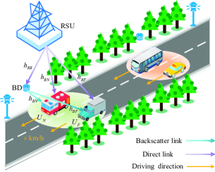
In this work, we consider an AmBC-NOMA-assisted high-mobility V2X scenario as depicted in Fig. 1, which consists of a roadside unit (RSU), a BD, a near vehicular user (denoted by ), and a far vehicular user (denoted by ).111Due to the strong interference between users, it may be challenging to jointly apply NOMA to all users in practice. A feasible alternative is to divide users into orthogonal pairs, where each pair performs NOMA. Therefore, this letter focuses on a typical NOMA user pair to illustrate the effectiveness of the proposed scheme. All the nodes are equipped with single antenna.
II-A High-mobility and Time-selective Channel Modeling
It is assumed that all channels are subject to Rayleigh fading,222This assumption is widely used in AmBC-NOMA V2X networks [7, 8, 9, 10, 11]. and the channel coefficients from RSU to , , and BD are respectively denoted by , , and . Similarly, the channel coefficients from BD to and are respectively denoted by and . The aforementioned represents the average channel power.
For convenience, we assume that users are driving in the same direction with speed km/h on a highway. Due to the high-mobility nature of users, the corresponding fading channel () is assumed to be time-selective.333 Notably, since the BD is pre-positioned at a fixed location, we assume that is static, so that we do not consider imperfect CSI for it. To model the channel variation over time, the first-order auto-regressive process [12] is employed, and over the -th time instant can be described as
| (1) |
where is the time-varying component of the channel, and is the correlation parameter according to Jakes’ model. Specifically, we have . Here is the zeroth-order Bessel function of the first kind, is the transmitted symbol duration, and is the Doppler frequency shift for the vehicle with speed , where represents the carrier frequency and is the speed of light.
Time-selective undergoes rapid changes, posing significant challenges for receivers to achieve perfect channel estimation. Furthermore, real-time tracking of these channels is difficult, making it hard for receivers to estimate the channel at every time instant. Therefore, in this scenario, we assume that only estimate the CSI at the first time instant of each coherence time [12]. Using the minimum mean square error (MMSE) model, can be expressed as
| (2) |
where is the estimated CSI, is the estimation error. With the aid of (1) and (2), we can achieve [12, 13]:
| (3) |
where represents user mobility noise and follows the distribution .
For calculation convenience, we define as the effective noise caused by estimation error and user mobility. Obviously, is a complex Gaussian variable following , where , then (3) be rewritten as
| (4) |
II-B Transmission Model
Utilizing the NOMA protocol, the RSU transmits a superimposed signal to and , where is the total transmit power; and respectively denote the intended signals for and , with ; and are respectively the power coefficients allocated to and with and .
At the same time, the BD backscatters the RSU’s signal to users with its own message , where . The signals received by and are respectively given by
| (5) |
and
| (6) |
where denotes the reflection efficiency of BD; and respectively represent the additive white Gaussian noises (AWGNs) at and .
Unlike conventional NOMA, under the AmBC-NOMA protocol, first decodes , then decodes , and finally decodes . The above process can be achieved by using SIC technique. The received SINRs of , , and at can be respectively written as
| (7) |
| (8) |
and
| (9) |
where represents transmit signal-to-noise ratio (SNR), , , , and .
Meanwhile, only decodes by treating other signals as noise, whose SINR can be written as
| (10) |
where , , , and .
III The Statistics of SINRs
To obtain the theoretical expressions for BLER, we have to first explore the statistics of received SINRs. Specifically, the exact expressions of CDFs for different SINRs are summarized in the following lemmas.
Lemma 1.
The CDF of received SINR () can be derived as
| (11) |
where , , and
Proof.
See Appendix A. ∎
Lemma 2.
The CDF of received SINR can be derived as
| (12) |
where , , and
Proof.
The proof is similar to Appendix A, and thus omitted here due to space limitation. ∎
Lemma 3.
The CDF of received SINR can be derived as
| (13) |
where and .
Proof.
See Appendix B. ∎
IV BLER Analysis
In this section, we present the BLER analysis of the proposed system. For convenience, bit/s/Hz () is used to denote the maximum achievable rate of , with a blocklength of bits. The instantaneous BLER corresponding to the SINR () decoding in SPC ( bits) can be expressed as [16]
| (14) |
where is the Shannon capacity, and represents the channel dispersion. Since obtaining a closed-form solution for the current form of is highly challenging, we adopt the linear approach described in [17] to tightly approximate the above -function, i.e., (14), as
| (15) |
where , , , and . Then, the average BLER can be calculated as
| (16) |
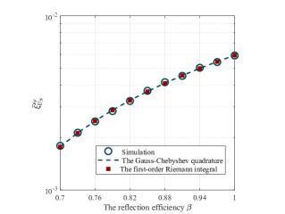
Recall that involves the product of (or ) and , making it challenging to obtain a closed-form expression for the integral. To evaluate this integral, we can employ the first-order Riemann integral444This method can be used when the integral interval is small. [18], i.e., , then (IV) becomes or we can employ the Gauss-Chebyshev quadrature method [15], resulting in
| (17) |
where represents the calculation accuracy, and
The accuracy of these two approximations is demonstrated in Fig. 2, shown at the top of previous page. It can be seen that both approximations exhibit high precision. Therefore, we herein adopt the simpler approximation method, i.e., the first-order Riemann integral, to obtain the approximations. Subsequently, we can achieve the following theorems.
Theorem 1.
Proof.
See Appendix C. ∎
Theorem 2.
The approximated expression for e2e average BLER at can be derived as
| (20) |
when ; otherwise, ; , , and have been defined in Lemma 1.
V Numerical Results
In this section, we verify the accuracy of theoretical expressions through Monte Carlo methods. Unless otherwise stated, the simulation parameters are set as follows [8, 9, 19, 20, 21]: Power allocation coefficients and ; time instant index ; carrier frequency GHz; transmitted symbol duration ms; vehicle speed km/h; blocklength of different streams bits; bit/s/Hz and bit/s/Hz; variances of different channels , , , , and ; error levels of different channels ; reflection efficiency .
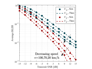
In Fig. 5, we present the average BLERs versus the transmit SNR with different vehicle speeds . The theoretical results of the average BLER performance exhibit good agreement with the simulated ones. As seen from Fig. 5, all the curves steadily decrease as increases. It is evident that higher speed levels degrade the performance of both users, since mobility can seriously interfere the estimated CSI at -th time instant. On the other hand, we find that the BLER of is always worse than that of , which is determined by the different SIC processes for the two users. Specifically, needs to successively decode three signals, while only needs to decode its own signal, leading to higher BLER for .
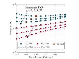
Fig. 5 illustrates the relationship between average BLER and the reflection efficiency with different transmit SNR levels. It’s evident that larger values correspond to larger SINRs, resulting in a decrease in average BLER as increases. Besides, regarding the average BLER of , it increases with increasing due to larger interference caused by the backscatter link. Conversely, for the average BLER of , it initially decreases to an optimal point and then increases with increasing . This is because with a smaller , the power of backscattered by BD is lower, causing larger , and finally resulting in poor BLER performance. However, as becomes larger, the enhancement of cannot eliminate the growth of interference caused by the backscatter link in and . Therefore, choosing an appropriate reflection efficiency is crucial.
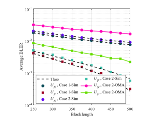
The average BLERs of different schemes versus blocklength when dB for different cases is plotted in Fig. 5, with for Case 1 and for Case 2. It can be observed that with increasing blocklength, the average BLER decreases. Clearly, AmBC-NOMA always exhibits better average BLER performance than the OMA counterpart, corroborating its capability of providing higher SE. Therefore, employing AmBC-NOMA in high-mobility communication is highly beneficial. Additionally, we find that higher levels of CSI error leads to a deterioration in the BLER performance. Hence, maintaining accurate CSI in high-mobility scenario is a critical requirement for achieving better BLER performance.
VI Conclusions
In this paper, we have proposed a two-user AmBC-NOMA-assisted high-mobility V2X system over time-selective fading channels under CSI imperfections. The derived theoretical expressions for the BLERs have effectively characterized the system’s performance. Simulation results have validated the accuracy of theoretical results and showed the impacts of different transmit SNRs, CSI imperfections, vehicle speeds, reflection efficiency coefficients, and blocklength on the BLER. Finally, simulation results have shown that the proposed AmBC-NOMA system outperforms the AmBC-OMA counterpart.
Appendix A Proof of Lemma 1
Appendix B Proof of Lemma 3
Appendix C Proof of Theorem 1
For convenience, let
| (C.1a) | ||||
| (C.1b) | ||||
| (C.1c) | ||||
Apparently, we have , , and . Utilizing the aforementioned equations and after performing some mathematical operations, can be converted to
| (C.2) |
Then, by substituting (C.1a), (C.1b), and (C.1c) into the above equation, we can derive the approximated expressions of , completing the proof.
References
- [1] M. Noor-A-Rahim, Z. Liu, H. Lee, M. O. Khyam, J. He, D. Pesch, K. Moessner, W. Saad, and H. V. Poor, “6G for vehicle-to-everything (V2X) communications: Enabling technologies, challenges, and opportunities,” Proc. IEEE, vol. 110, no. 6, pp. 712–734, 2022.
- [2] B. Di, L. Song, Y. Li, and Z. Han, “V2X meets NOMA: Non-orthogonal multiple access for 5G-enabled vehicular networks,” IEEE Wireless Commun., vol. 24, no. 6, pp. 14–21, 2017.
- [3] X. Lai, Q. Zhang, and J. Qin, “Cooperative NOMA short-packet communications in flat Rayleigh fading channels,” IEEE Trans. Veh. Technol., vol. 68, no. 6, pp. 6182–6186, 2019.
- [4] V. Liu, A. Parks, V. Talla, S. Gollakota, D. Wetherall, and J. R. Smith, “Ambient backscatter: Wireless communication out of thin air,” ACM SIGCOMM Comput. Commun. Rev, vol. 43, no. 4, pp. 39–50, 2013.
- [5] G. Yang, Q. Zhang, and Y.-C. Liang, “Cooperative ambient backscatter communications for green Internet-of-Things,” IEEE Internet Things J., vol. 5, no. 2, pp. 1116–1130, 2018.
- [6] Q. Zhang, L. Zhang, Y.-C. Liang, and P.-Y. Kam, “Backscatter-NOMA: A symbiotic system of cellular and Internet-of-Things networks,” IEEE Access, vol. 7, pp. 20 000–20 013, 2019.
- [7] W. U. Khan, F. Jameel, N. Kumar, R. Jäntti, and M. Guizani, “Backscatter-enabled efficient V2X communication with non-orthogonal multiple access,” IEEE Trans. Veh. Technol., vol. 70, no. 2, pp. 1724–1735, 2021.
- [8] Y. Zheng, X. Li, H. Zhang, M. D. Alshehri, S. Dang, G. Huang, and C. Zhang, “Overlay cognitive ABCom-NOMA-based ITS: An in-depth secrecy analysis,” IEEE Trans. Intell. Transp. Syst., vol. 24, no. 2, pp. 2217–2228, 2022.
- [9] W. U. Khan, M. A. Jamshed, E. Lagunas, S. Chatzinotas, X. Li, and B. Ottersten, “Energy efficiency optimization for backscatter enhanced NOMA cooperative V2X communications under imperfect CSI,” IEEE Trans. Intell. Transp. Syst., vol. 24, no. 11, pp. 12 961–12 972, 2023.
- [10] H. Peng, M. Liu, L. Yang, M. Zeng, J. Wang, K. Guo, and X. Li, “Ambient backscatter communication symbiotic intelligent transportation systems: Covertness performance analysis and optimization,” IEEE Trans. Consum. Electron., 2023.
- [11] A. Ihsan, W. Chen, W. U. Khan, Q. Wu, and K. Wang, “Energy-efficient backscatter aided uplink NOMA roadside sensor communications under channel estimation errors,” IEEE Trans. Intell. Transp. Syst., vol. 24, no. 5, pp. 4962–4974, 2023.
- [12] Y. M. Khattabi and M. M. Matalgah, “Performance analysis of multiple-relay AF cooperative systems over Rayleigh time-selective fading channels with imperfect channel estimation,” IEEE Trans. Veh. Technol., vol. 65, no. 1, pp. 427–434, 2015.
- [13] C. Xia, Z. Xiang, J. Meng, H. Liu, and G. Pan, “NOMA-assisted cognitive short-packet communication with node mobility and imperfect channel estimation,” IEEE Trans. Veh. Technol., vol. 72, no. 9, pp. 12 276–12 287, 2023.
- [14] G. Durisi, T. Koch, and P. Popovski, “Toward massive, ultrareliable, and low-latency wireless communication with short packets,” Proc. IEEE, vol. 104, no. 9, pp. 1711–1726, 2016.
- [15] I. S. Gradshteyn and I. M. Ryzhik, Table of Integrals, Series, and Products. Academic press, 2007.
- [16] W. Yang, G. Durisi, T. Koch, and Y. Polyanskiy, “Quasi-static multiple-antenna fading channels at finite blocklength,” IEEE Trans. Inf. Theory, vol. 60, no. 7, pp. 4232–4265, 2014.
- [17] B. Makki, T. Svensson, and M. Zorzi, “Finite block-length analysis of the incremental redundancy HARQ,” IEEE Wireless Commun. Lett., vol. 3, no. 5, pp. 529–532, 2014.
- [18] C. D. Ho, T.-V. Nguyen, T. Huynh-The, T.-T. Nguyen, D. B. da Costa, and B. An, “Short-packet communications in wireless-powered cognitive IoT networks: Performance analysis and deep learning evaluation,” IEEE Trans. Veh. Technol., vol. 70, no. 3, pp. 2894–2899, 2021.
- [19] J. Zhu, Y. Chen, X. Pei, T. Pei, X. Li, and T. A. Tsiftsis, “Rate-splitting multiple access with finite blocklength and high mobility for URLLC transmissions,” IEEE Wireless Commun. Lett., 2024.
- [20] X. Li, M. Zhao, M. Zeng, S. Mumtaz, V. G. Menon, Z. Ding, and O. A. Dobre, “Hardware impaired ambient backscatter NOMA systems: Reliability and security,” IEEE Trans. Commun., vol. 69, no. 4, pp. 2723–2736, 2021.
- [21] T.-H. Vu, T.-V. Nguyen, T.-T. Nguyen, and S. Kim, “Performance analysis and deep learning design of wireless powered cognitive NOMA IoT short-packet communications with imperfect CSI and SIC,” IEEE Internet Things J., vol. 9, no. 13, pp. 10 464–10 479, 2021.