On Sequential Loss Approximation for Continual Learning
Abstract
We introduce for continual learning Autodiff Quadratic Consolidation (AQC), which approximates the previous loss function with a quadratic function, and Neural Consolidation (NC), which approximates the previous loss function with a neural network. Although they are not scalable to large neural networks, they can be used with a fixed pre-trained feature extractor. We empirically study these methods in class-incremental learning, for which regularization-based methods produce unsatisfactory results, unless combined with replay. We find that for small datasets, quadratic approximation of the previous loss function leads to poor results, even with full Hessian computation, and NC could significantly improve the predictive performance, while for large datasets, when used with a fixed pre-trained feature extractor, AQC provides superior predictive performance. We also find that using tanh-output features can improve the predictive performance of AQC. In particular, in class-incremental Split MNIST, when a Convolutional Neural Network (CNN) with tanh-output features is pre-trained on EMNIST Letters and used as a fixed pre-trained feature extractor, AQC can achieve predictive performance comparable to joint training.
1 Introduction
Continual learning, also known as incremental learning or lifelong learning, is learning from a sequence of datasets called tasks which are not necessarily identically distributed. When a neural network (including a generalized linear model, which is essentially a neural network with no hidden layers) is trained on a task and fine-tuned on a new task, it loses predictive performance on the old task. This phenomenon is known as catastrophic forgetting [1] and can be prevented by joint training on all tasks, but previous data may not be accessible due to computational or privacy constraints. Thus, the goal of continual learning is to prevent catastrophic forgetting without accessing previous data.
Continual-learning settings vary considerably, and three main types are commonly studied [2]:
-
1.
Task-incremental learning, in which task IDs are provided and the classes change between tasks
-
2.
Domain-incremental learning, in which task IDs are not provided and the classes remain the same between tasks
-
3.
Class-incremental learning, in which task IDs are not provided and the classes change between tasks
Multi-headed models, in which there is one output head for each task, are commonly used for task-incremental learning. However, task-incremental learning has been criticized as task IDs make the problem of continual learning easier [3]. In fact, if there is only one class per task, then the task ID could be used to make a perfect prediction. In accordance with the desiderata proposed in [3], we focus on class-incremental learning with single-headed models on more than two similar tasks with no access to previous data.
Sequential Bayesian inference provides an elegant approach to continual learning. We assume that the parameters of the model are random and use the previous posterior Probability Density Function (PDF) as the current prior PDF. For Maximum-A-Posteriori (MAP) prediction, this can be formulated as sequential loss approximation. In this work, we use Autodiff Quadratic Consolidation (AQC), which approximates the previous loss function with a quadratic function, and Neural Consolidation (NC), which approximates the previous loss function with a neural network. Since these methods are not scalable to large models with millions of parameters, we use a fixed pre-trained feature extractor for image datasets. We show empirically that for small datasets, neural-network approximation of the previous loss function leads to significant improvements in predictive performance over quadratic approximation of the previous loss function and that using tanh-output features improves the predictive performance of AQC.
2 Sequential Bayesian inference and sequential loss approximation
Let be the parameters of the neural network, be the input data from time to and be the output data from time to . The independence assumptions are described by the following Bayesian network. In particular, are assumed to be independent, and given and , are assumed to be conditionally independent.
For , represents a task or dataset at time , and the individual points in each task are assumed to be independent and identically distributed.
Tasks are assumed to be similar, so the likelihood PDF at time , , is assumed to be the same for all tasks. It is defined by the neural network, which maps to some parameters of . In binary classification, is Bernoulli, and the neural network maps to the log-probability of the positive class, while in multi-class classification, is categorical, and the neural network maps to the un-normalized log-probabilities of the classes. The posterior PDF at time , , can be obtained by recursive application of Bayes’ rule, where the posterior PDF at time is used as the prior PDF at time :
where is a normalization term that does not depend on .
MAP prediction uses the maximum of the posterior PDF at time to make a point prediction. Since normalizing constants do not affect the maximum, is also equal to the maximum of the joint PDF . Maximizing the PDF is equivalent to minimizing the negative log PDF. Thus, the total loss at time could be defined as and the task loss at time as . This leads to a recursion of loss functions for :
Methods based on this recursion are also known as regularization-based methods as can be seen as regularizing . Note that , the negative log prior, may be in un-normalized form. In particular, a Gaussian prior PDF with zero mean vector and covariance matrix corresponds to an regularization term . In binary classification, is the sigmoid cross-entropy loss, while in multi-class classification, is the softmax cross-entropy loss.
2.1 Autodiff quadratic consolidation
Quadratic approximation of corresponds to Laplace approximation of the previous posterior PDF and requires computing the minimum and its Hessian matrix at the minimum. Since the Hessian operator is linear, successive quadratic approximation results in addition of the Hessian matrices of the previous tasks:
Autodiff Quadratic Consolidation (AQC) computes Hessian matrices by using automatic differentiation. The computational cost depends on the size of the model, i.e. the number of the parameters , and the size of the dataset. If the model is small but the dataset is large, the computation can be made tractable by computing in mini-batches. Since the Hessian operator is linear, the Hessian matrix of the batch loss function is equal to the sum of the Hessian matrices of the mini-batch loss functions. If are the mini-batch loss functions corresponding to the batch loss function , then
2.2 Neural consolidation
Neural Consolidation (NC) uses a consolidator neural network with parameters to approximate :
After finding the minimum , the consolidator neural network is trained by using mini-batch gradient descent. At each step, a sample of points are generated randomly and uniformly within a ball of radius around , and the consolidator loss function is minimized to obtain :
where is an regularization factor, and each is the Huber loss:
If the dataset is large, the true loss values can be computed by adding the mini-batch loss values.
2.3 Limitations
In sequential loss approximation, the total number of classes must be known in advance, even if the classes are learned incrementally, so that the number of parameters is fixed. Otherwise, the assumptions made above will be violated and sequential Bayesian inference will no longer be valid.
AQC and NC are local approximations, so if the minimum moves very far when learning a new task, the approximation will not be very accurate. NC is also sensitive to hyperparameters such as the radius , the sample size and the architecture of the consolidator neural network. These algorithms do not scale with model size, but the model size can be reduced by using a fixed pre-trained feature extractor. On the other hand, they scale with dataset size, and memory-mapped files can be used to increase the efficiency of the algorithms.
3 Related work
There are several works using quadratic approximation of the previous loss function. Elastic Weight Consolidation (EWC) approximates the Hessian matrix by using a diagonal Fisher information matrix, which is computed by averaging the squared gradients over mini-batches [4]. However, it adds a penalty term for every new task, and [5] points out that it is not well justified and that the penalty term can be updated by adding the Hessian matrices. Synpatic Intelligence (SI) also performs a diagonal approximation of the Hessian. However, it does so by using the change in loss during gradient descent, which is computed by summing the product of the gradient and the change in the parameter values during gradient descent [6]. Online Structured Laplace Approximation (OSLA) uses Kronecker factorization to perform a block-diagonal approximation of the Hessian, in which the diagonal blocks of the matrix correspond to a layer of the neural network [7].
The above methods are designed to be scalable to large models and have mainly been shown to perform well in Permuted MNIST [8], with OSLA performing better than EWC and SI. In class-incremental Split MNIST, EWC and SI have been shown to perform as poorly as fine-tuning [2]. It has also been observed that regularization-based methods generally perform worse than replay-based methods, which use stored or generated previous data [9, 2]. In our work, we examine how much predictive performance we can achieve by using a full Hessian computation and whether the quadratic approximation can be improved by approximation with a neural network, which is a powerful function approximator.
Recently, two types of pre-training have been studied for continual learning: pre-training for initialization and pre-training for feature extraction. In the former, the parameters of the neural network are initialized with the pre-trained parameters rather than randomly, which has been reported to reduce forgetting [10, 11]. In the latter, a pre-trained model is used as a feature extractor, which has also been reported to reduce forgetting [12, 13, 14]. Intuitively, neural networks do not need to learn lower-level features continually as much as they need to learn higher-level features, just as humans do not need to learn continually to recognize edges, corners and shapes as much as they need to learn to recognize objects. It has also been empirically shown that forgetting is more pronounced in later layers of a neural network [15]. Thus, in our work, we use pre-training for feature extraction for image datasets.
4 Experiments
In our experiments, we compare EWC, SI, AQC and NC in class-incremental-learning settings based on small and large datasets. For EWC, we use the variant with Huszár’s corrected penalty [5] and the Fisher information matrix, which is computed based on the empirical distribution of and the conditional distribution of given defined by the model (rather than the empirical Fisher information matrix, which is computed based on the empirical distribution of and ) [16].
The experiments are run on an on-premise NVIDIA GeForce RTX 4090 GPU with 24 GB of memory. In every experiment, swish activation functions are used except in some pre-trained neural networks with tanh activation functions before the final layer, the regularization factor is and optimization is done by using the Adam optimizer with learning rate 0.01. For Split Iris and Split Wine, the datasets are split randomly with 80% for training and 20% for testing, while for Split MNIST and Split CIFAR-10, the original dataset splits are used. Then, the each split dataset is split by class into multiple tasks. For NC, hyperparameters are chosen by manual tuning, while for EWC and SI, they are fixed at and , respectively. Evaluation is done by using the average accuracy, which is the average of testing accuracy scores of the tasks up to and including the current task.
4.1 Split Iris
Iris is a dataset consisting of 150 instances of flowers with 4 features (sepal length, sepal width, petal length and petal width) and a 3-class label (setosa, versicolor and virginica), and Split Iris splits the dataset into 3 tasks by class. Before evaluating on Split Iris, we visualize loss functions by using Split Iris 1, which consists of one feature (petal length) and a binary label indicating whether the species is virginica or not, and predictions by using Split Iris 2, which consists of two features (petal length and petal width) and a 3-class label.
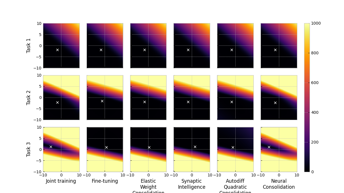
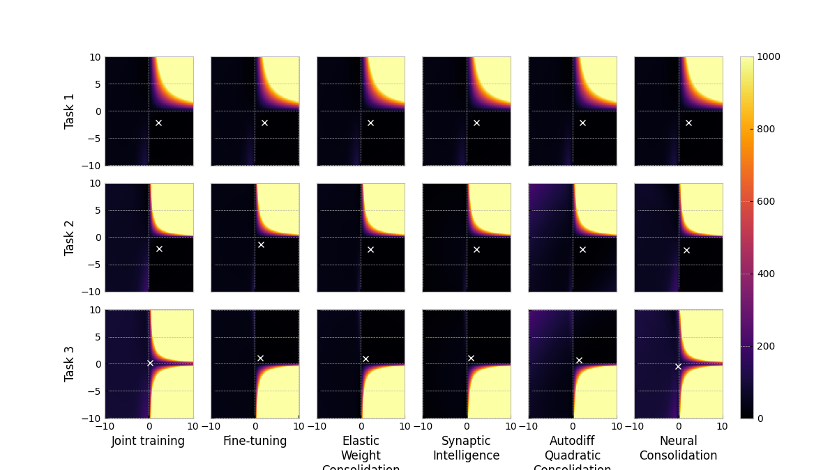
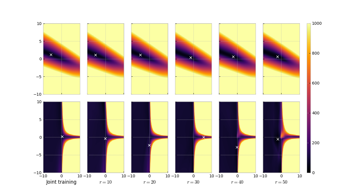
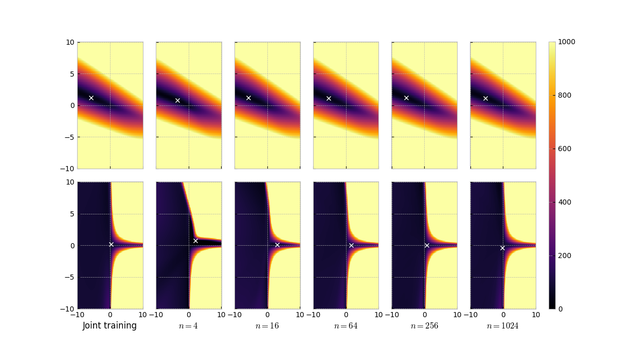
For Split Iris 1, we use two 2-parameter models for convenience of visualization of loss functions: a logistic-regression model, for which the consolidator neural network has two hidden layers each of 50 nodes, and a neural network with one hidden layer of one node and no bias, for which the consolidator neural network has two hidden layers each of 200 nodes. NC is done with radius and sample size . The visualization of the loss functions is shown in Figure 1, and the visualization of the final loss functions under different values of the radius and sample size is shown in Figure 2. It can be seen that NC could approximate the loss functions significantly better than EWC, SI and AQC, but NC is sensitive to hyperparameters such as the radius and the sample size .
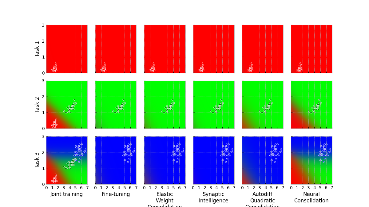
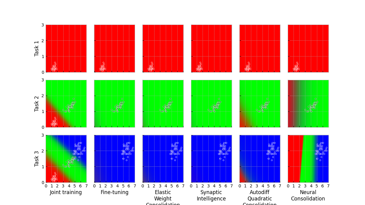
For Split Iris 2, we use the following two models: a softmax-regression model, for which the consolidator neural network has two hidden layers each of 50 nodes, and a neural network with one hidden layer of 3 nodes, for which the consolidator neural network has two hidden layers each of 200 nodes. NC is done with radius and sample size . The visualizations of the predictions are shown in Figure 3. It can be seen that the predictions of NC are better than those of EWC, SI and AQC, especially on the softmax-regression model. The loss function of a neural network is much more difficult to fit, so the results of NC on the neural network are not as good as those on the softmax-regression model.
For Split Iris, we use the following two models: a softmax-regression model, for which the consolidator neural network has two hidden layers each of 50 nodes, and a neural network with one hidden layer of one node and no bias, for which the consolidator neural network has two hidden layers each of 200 nodes. NC is done with radius and sample size . The results are shown in Table 1. It can be seen that EWC, SI and AQC perform as poorly as fine-tuning, and NC outperforms them significantly.
| Method | Task 1 | Task 2 | Task 3 |
|---|---|---|---|
| Softmax-regression model | |||
| Joint training | 100.00 | 100.00 | 100.00 |
| Fine-tuning | 100.00 | 50.00 | 33.33 |
| EWC | 100.00 | 50.00 | 33.33 |
| SI | 100.00 | 50.00 | 33.33 |
| AQC | 100.00 | 50.00 | 33.33 |
| NC | 100.00 | 100.00 | 93.33 |
| Neural network | |||
| Joint training | 100.00 | 100.00 | 100.00 |
| Fine-tuning | 100.00 | 50.00 | 33.33 |
| EWC | 100.00 | 50.00 | 33.33 |
| SI | 100.00 | 50.00 | 33.33 |
| AQC | 100.00 | 50.00 | 33.33 |
| NC | 100.00 | 100.00 | 100.00 |
4.2 Split Wine
Wine is a dataset consisting of 178 instances of wine each with 13 features and a 3-class label, and Split Wine splits the dataset into 3 tasks by class. We use the following two models: a softmax-regression model, for which the consolidator neural network has two hidden layers each of 50 nodes, and a neural network with one hidden layer of 3 nodes, for which the consolidator neural network has two hidden layers each of 2000 nodes. NC is done with radius and sample size . The results are shown in Table 2. It can be seen that EWC, SI and AQC perform as poorly as fine-tuning, and NC outperform them significantly on the softmax-regression model, but on the neural network, NC performs well only up to the second task.
| Method | Task 1 | Task 2 | Task 3 |
|---|---|---|---|
| Softmax-regression model | |||
| Joint training | 100.00 | 97.06 | 95.01 |
| Fine-tuning | 100.00 | 50.00 | 33.33 |
| EWC | 100.00 | 50.00 | 33.33 |
| SI | 100.00 | 50.00 | 33.33 |
| AQC | 100.00 | 50.00 | 33.33 |
| NC | 100.00 | 94.12 | 76.08 |
| Neural network | |||
| Joint training | 100.00 | 97.06 | 91.68 |
| Fine-tuning | 100.00 | 50.00 | 33.33 |
| EWC | 100.00 | 50.00 | 33.33 |
| SI | 100.00 | 50.00 | 33.33 |
| AQC | 100.00 | 50.00 | 33.33 |
| NC | 100.00 | 91.18 | 33.33 |
4.3 Split MNIST
MNIST is a dataset consisting of 60,000 instances of handwritten digits with a image and a 10-class label [17]. Split MNIST splits the dataset into 5 tasks, the first consisting of 1’s and 2’s, the second consisting of 3’s and 4’s and so on. EMNIST Letters consists of 26 classes of images of handwritten letters in both upper case and lower case [18] and has no class overlap with MNIST.
We pre-train two Convolutional Neural Networks (CNNs) on EMNIST Letters and use them as fixed feature extractors. Each consists of a convolutional layer of 32 filters, an average-pooling layer with a stride of 2, a convolutional layer of 32 filters, an average-pooling layer with a stride of 2, a dense layer of 32 nodes and finally a dense layer of 26 nodes. Features are extracted before the final layer, and in that layer, one CNN uses swish activation functions, while the other uses tanh activation functions.
For Split MNIST, we use the pre-trained CNNs to extract features and perform continual learning on a dense layer with 10 nodes, for which the consolidator neural network has two hidden layers each of 5000 nodes. NC is done with radius and sample size . It can be seen that AQC outperforms NC, EWC and SI, in both cases. Notably, using tanh-output features significantly reduces forgetting in EWC, SI, AQC and NC although it also slightly reduces the final average accuracy in joint training. In particular, AQC achieves performance comparable to joint training.
| Method | Task 1 | Task 2 | Task 3 | Task 4 | Task 5 |
|---|---|---|---|---|---|
| Feature extractor with swish output | |||||
| Joint training | 100.00 | 98.63 | 98.60 | 97.04 | 95.06 |
| Fine-tuning | 100.00 | 49.22 | 33.32 | 24.96 | 19.54 |
| EWC | 100.00 | 49.22 | 33.32 | 24.96 | 19.54 |
| SI | 100.00 | 49.22 | 33.32 | 24.96 | 19.54 |
| AQC | 100.00 | 96.14 | 81.04 | 61.79 | 47.55 |
| NC | 100.00 | 56.05 | 45.75 | 33.29 | 26.23 |
| Feature extractor with tanh output | |||||
| Joint training | 99.86 | 98.54 | 98.13 | 96.43 | 93.66 |
| Fine-tuning | 99.86 | 49.29 | 33.85 | 24.96 | 19.69 |
| EWC | 99.86 | 76.43 | 57.72 | 40.33 | 26.03 |
| SI | 99.86 | 76.31 | 57.27 | 39.41 | 25.33 |
| AQC | 99.86 | 98.52 | 97.96 | 96.11 | 92.26 |
| NC | 99.86 | 85.26 | 57.68 | 43.34 | 34.79 |
4.4 Split CIFAR-10
We pre-train two CNNs on CIFAR-100 and use them as fixed feature extractors. Each consists of two convolutional layers of 128 filters, an average-pooling layer with a stride of 2, two convolutional layers of 256 filters, an average-pooling layer with a stride of 2, a dense layer of 256 nodes, a dense layer of 128 nodes and finally a dense layer of 100 nodes. Features are extracted before the final layer, and in that layer, one CNN uses swish activation functions, while the other uses tanh activation functions.
For Split CIFAR-10, we use the pre-trained CNNs to extract features and perform continual learning on a dense layer with 10 nodes, for which the consolidator neural network has two hidden layers each of 5000 nodes. NC is done with radius and sample size . As in Split MNIST, it can be seen that AQC outperforms NC, EWC and SI, in both cases. Using tanh-output features significantly reduces forgetting only in AQC.
| Method | Task 1 | Task 2 | Task 3 | Task 4 | Task 5 |
|---|---|---|---|---|---|
| Feature extractor with swish output | |||||
| Joint training | 89.45 | 73.28 | 57.27 | 52.35 | 50.10 |
| Fine-tuning | 89.45 | 37.95 | 26.70 | 22.90 | 16.75 |
| EWC | 89.45 | 37.93 | 26.70 | 22.90 | 17.57 |
| SI | 89.45 | 37.95 | 26.70 | 22.90 | 16.77 |
| AQC | 89.45 | 47.58 | 31.98 | 26.10 | 21.03 |
| NC | 89.45 | 49.15 | 22.46 | 19.53 | 11.21 |
| Feature extractor with tanh output | |||||
| Joint training | 88.50 | 71.80 | 57.23 | 52.35 | 48.50 |
| Fine-tuning | 88.50 | 37.03 | 26.67 | 22.56 | 16.88 |
| EWC | 88.50 | 38.75 | 26.8 | 22.60 | 20.85 |
| SI | 88.50 | 37.95 | 26.72 | 22.59 | 19.22 |
| AQC | 88.50 | 61.63 | 45.08 | 40.53 | 39.24 |
| NC | 88.50 | 5.40 | 5.45 | 8.36 | 8.05 |
4.5 Data availability
All the datasets used in this paper are publicly available. Iris and Wine are available from the scikit-learn package [20], which is released under the 3-clause BSD license. MNIST, EMNIST, CIFAR-10 and CIFAR-100 are available from the pytorch package [21], which is also released under the 3-clause BSD license.
4.6 Code availability
Documented code for the experiments is available online under an MIT licence: https://github.com/blackblitz/bcl. Reproducibility is ensured by fixing the seed in pseudo-random-number generation and using deterministic GPU algorithms. Detailed instructions to reproduce the results are provided in the README file of the repository.
5 Conclusion
We proposed Autodiff Quadratic Consolidation (AQC) and Neural Consolidation (NC) for continual learning based on sequential loss approximation. Although they are not scalable to very large neural networks, they can be used together with fixed pre-trained feature extractors. In class-incremental learning settings with small datasets, methods based on quadratic approximation of the loss function, such as EWC, SI and AQC, perform as poorly as fine-tuning, and NC performs better. With large datasets, when used with pre-training, AQC performs very well and its performance can be improved by using tanh-output features, probably because the output of the tanh function is between -1 and 1, leading to a loss function that can be better approximated with a quadratic function.
NC is conceptually appealing as neural networks are much more powerful function approximators than quadratic functions. However, in practice, it is difficult to tune the hyperparameters. One possible reason that it does not work well with large datasets is that larger datasets lead to steeper loss functions, which may affect gradient descent. Moreover, although we have access to the loss function to be approximated, we need to take a sample of points from it to train the consolidator neural network. It would be better if we could fit directly to the loss function without generating a sample of points.
We hope that our work provides some insights on sequential loss approximation for continual learning.
Acknowledgments and Disclosure of Funding
We thank Pengcheng Hao, Yang Li and anonymous reviewers for their feedback.
References
- [1] Michael McCloskey and Neal J. Cohen “Catastrophic Interference in Connectionist Networks: The Sequential Learning Problem” In Psychology of Learning and Motivation - Advances in Research and Theory 24, 1989 DOI: 10.1016/S0079-7421(08)60536-8
- [2] Gido M. Ven, Tinne Tuytelaars and Andreas S. Tolias “Three Types of Incremental Learning” In Nature Machine Intelligence 4.12, 2022, pp. 1185–1197 DOI: 10.1038/s42256-022-00568-3
- [3] Sebastian Farquhar and Yarin Gal “Towards Robust Evaluations of Continual Learning”, 2019 arXiv:1805.09733
- [4] James Kirkpatrick, Razvan Pascanu, Neil Rabinowitz, Joel Veness, Guillaume Desjardins, Andrei A. Rusu, Kieran Milan, John Quan, Tiago Ramalho, Agnieszka Grabska-Barwinska, Demis Hassabis, Claudia Clopath, Dharshan Kumaran and Raia Hadsell “Overcoming Catastrophic Forgetting in Neural Networks” In Proceedings of the National Academy of Sciences of the United States of America 114.13, 2017, pp. 3521–3526 DOI: 10.1073/pnas.1611835114
- [5] Ferenc Huszár “Note on the Quadratic Penalties in Elastic Weight Consolidation” In Proceedings of the National Academy of Sciences of the United States of America 115.11, 2018, pp. E2496–E2497 DOI: 10.1073/pnas.1717042115
- [6] Friedemann Zenke, Ben Poole and Surya Ganguli “Continual Learning Through Synaptic Intelligence” In Proceedings of the 34th International Conference on Machine Learning 70, Proceedings of Machine Learning Research PMLR, 2017, pp. 3987–3995 URL: https://proceedings.mlr.press/v70/zenke17a.html
- [7] Hippolyt Ritter, Aleksandar Botev and David Barber “Online Structured Laplace Approximations for Overcoming Catastrophic Forgetting” In Advances in Neural Information Processing Systems 31 Curran Associates, Inc., 2018 URL: https://proceedings.neurips.cc/paper_files/paper/2018/file/f31b20466ae89669f9741e047487eb37-Paper.pdf
- [8] Ian J. Goodfellow, Mehdi Mirza, Da Xiao, Aaron Courville and Yoshua Bengio “An Empirical Investigation of Catastrophic Forgetting in Gradient-Based Neural Networks”, 2015 arXiv:1312.6211
- [9] Zheda Mai, Ruiwen Li, Jihwan Jeong, David Quispe, Hyunwoo Kim and Scott Sanner “Online Continual Learning in Image Classification: An Empirical Survey” In Neurocomputing 469, 2022, pp. 28–51 DOI: https://doi.org/10.1016/j.neucom.2021.10.021
- [10] Kuan-Ying Lee, Yuanyi Zhong and Yu-Xiong Wang “Do Pre-Trained Models Benefit Equally in Continual Learning?” In Proceedings of the IEEE/CVF Winter Conference on Applications of Computer Vision (WACV), 2023, pp. 6485–6493
- [11] Sanket Vaibhav Mehta, Darshan Patil, Sarath Chandar and Emma Strubell “An Empirical Investigation of the Role of Pre-training in Lifelong Learning” In Journal of Machine Learning Research 24.214, 2023, pp. 1–50 URL: http://jmlr.org/papers/v24/22-0496.html
- [12] Wenpeng Hu, Qi Qin, Mengyu Wang, Jinwen Ma and Bing Liu “Continual Learning by Using Information of Each Class Holistically”, 2021, pp. 7797–7805 DOI: 10.1609/aaai.v35i9.16952
- [13] Xiaojie Li, Haifeng Li and Lin Ma “Continual Learning of Medical Image Classification Based on Feature Replay” In 2022 16th IEEE International Conference on Signal Processing (ICSP) 1, 2022, pp. 426–430 DOI: 10.1109/ICSP56322.2022.9965230
- [14] Yang Yang, Zhiying Cui, Junjie Xu, Changhong Zhong, Wei-Shi Zheng and Ruixuan Wang “Continual Learning with Bayesian Model Based on a Fixed Pre-trained Feature Extractor” In Visual Intelligence 1.1, 2023, pp. 5 DOI: 10.1007/s44267-023-00005-y
- [15] Xialei Liu, Chenshen Wu, Mikel Menta, Luis Herranz, Bogdan Raducanu, Andrew D. Bagdanov, Shangling Jui and Joost van Weijer “Generative Feature Replay for Class-Incremental Learning” In Proceedings of the IEEE/CVF Conference on Computer Vision and Pattern Recognition (CVPR) Workshops, 2020
- [16] James Martens “New insights and perspectives on the natural gradient method” In Journal of Machine Learning Research 21.146, 2020, pp. 1–76
- [17] Y. Lecun, L. Bottou, Y. Bengio and P. Haffner “Gradient-based learning applied to document recognition” In Proceedings of the IEEE 86.11, 1998, pp. 2278–2324 DOI: 10.1109/5.726791
- [18] Gregory Cohen, Saeed Afshar, Jonathan Tapson and André Schaik “EMNIST: Extending MNIST to handwritten letters” In 2017 International Joint Conference on Neural Networks (IJCNN), 2017, pp. 2921–2926 DOI: 10.1109/IJCNN.2017.7966217
- [19] Alex Krizhevsky and Geoffrey Hinton “Learning multiple layers of features from tiny images” Toronto, ON, Canada, 2009
- [20] F. Pedregosa, G. Varoquaux, A. Gramfort, V. Michel, B. Thirion, O. Grisel, M. Blondel, P. Prettenhofer, R. Weiss, V. Dubourg, J. Vanderplas, A. Passos, D. Cournapeau, M. Brucher, M. Perrot and E. Duchesnay “Scikit-learn: Machine Learning in Python” In Journal of Machine Learning Research 12, 2011, pp. 2825–2830
- [21] Jason Ansel, Edward Yang, Horace He, Natalia Gimelshein, Animesh Jain, Michael Voznesensky, Bin Bao, Peter Bell, David Berard, Evgeni Burovski, Geeta Chauhan, Anjali Chourdia, Will Constable, Alban Desmaison, Zachary DeVito, Elias Ellison, Will Feng, Jiong Gong, Michael Gschwind, Brian Hirsh, Sherlock Huang, Kshiteej Kalambarkar, Laurent Kirsch, Michael Lazos, Mario Lezcano, Yanbo Liang, Jason Liang, Yinghai Lu, CK Luk, Bert Maher, Yunjie Pan, Christian Puhrsch, Matthias Reso, Mark Saroufim, Marcos Yukio Siraichi, Helen Suk, Michael Suo, Phil Tillet, Eikan Wang, Xiaodong Wang, William Wen, Shunting Zhang, Xu Zhao, Keren Zhou, Richard Zou, Ajit Mathews, Gregory Chanan, Peng Wu and Soumith Chintala “PyTorch 2: Faster Machine Learning Through Dynamic Python Bytecode Transformation and Graph Compilation” In 29th ACM International Conference on Architectural Support for Programming Languages and Operating Systems, Volume 2 (ASPLOS ’24) ACM, 2024 DOI: 10.1145/3620665.3640366