Causal-Aware Graph Neural Architecture Search under Distribution Shifts

Abstract

Graph neural architecture search (Graph NAS) has emerged as a promising approach for autonomously designing graph neural network architectures by leveraging the correlations between graphs and architectures. However, the existing methods fail to generalize under distribution shifts that are ubiquitous in real-world graph scenarios, mainly because the graph-architecture correlations they exploit might be spurious and varying across distributions. In this paper, we propose to handle the distribution shifts in the graph architecture search process by discovering and exploiting the causal relationship between graphs and architectures to search for the optimal architectures that can generalize under distribution shifts. The problem remains unexplored with the following critical challenges: 1) how to discover the causal graph-architecture relationship that has stable predictive abilities across distributions, 2) how to handle distribution shifts with the discovered causal graph-architecture relationship to search the generalized graph architectures. To address these challenges, we propose a novel approach, Causal-aware Graph Neural Architecture Search (CARNAS), which is able to capture the causal graph-architecture relationship during the architecture search process and discover the generalized graph architecture under distribution shifts. Specifically, we propose Disentangled Causal Subgraph Identification to capture the causal subgraphs that have stable prediction abilities across distributions. Then, we propose Graph Embedding Intervention to intervene on causal subgraphs within the latent space, ensuring that these subgraphs encapsulate essential features for prediction while excluding non-causal elements. Additionally, we propose Invariant Architecture Customization to reinforce the causal invariant nature of the causal subgraphs, which are utilized to tailor generalized graph architectures. Extensive experiments on synthetic and real-world datasets demonstrate that our proposed CARNAS achieves advanced out-of-distribution generalization ability by discovering the causal relationship between graphs and architectures during the search process.

1 Introduction

Graph neural architecture search (Graph NAS), aiming at automating the designs of GNN architectures for different graphs, has shown great success by exploiting the correlations between graphs and architectures. Present approaches [9, 19, 24] leverage a rich search space filled with GNN operations and employ strategies like reinforcement learning and continuous optimization algorithms to pinpoint an optimal architecture for specific datasets, aiming to decode the natural correlations between graph data and their ideal architectures. Based on the independently and identically distributed (I.I.D) assumption on training and testing data, existing methods assume the graph-architecture correlations are stable across graph distributions.

Nevertheless, distribution shifts are ubiquitous and inevitable in real-world graph scenarios, particularly evident in applications existing with numerous unforeseen and uncontrollable hidden factors like drug discovery, in which the availability of training data is limited, and the complex chemical properties of different molecules lead to varied interaction mechanisms [16]. Consequently, GNN models developed for such purposes must be generalizable enough to handle the unavoidable variations in data distribution between training and testing sets, underlining the critical need for models that can adapt to and perform reliably under such varying conditions.

However, existing Graph NAS methods fail to generalize under distribution shifts, since they do not specifically consider the relationship between graphs and architectures, and may exploit the spurious correlations between graphs and architectures unintendedly, which vary with distribution shifts, during the search process. Relying on these spurious correlations, the search process identifies patterns that are valid only in the training data but do not generalize to unseen data. This results in good performance on the training distribution but poor performance when the underlying data distribution changes in the test set.

In this paper, we study the problem of graph neural architecture search under distribution shifts by capturing the causal relationship between graphs and architectures to search for the optimal graph architectures that can generalize under distribution shifts. The problem is highly non-trivial with the following challenges: 1) How to discover the causal graph-architecture relationship that has stable predictive abilities across distributions? and 2) How to handle distribution shifts with the discovered causal graph-architecture relationship to search the generalized graph architectures?

To address these challenges, we propose the Causal-aware Graph NAS (CARNAS), which is able to capture the causal relationship, stable to distribution shifts, between graphs and architectures, and thus handle the distribution shifts in the graph architecture search process. Specifically, we design a Disentangled Causal Subgraph Identification module, which employs disentangled GNN layers to obtain node and edge representations, then further derive causal subgraphs based on the importance of each edge. This module enhances the generalization by deeply exploring graph features as well as latent information with disentangled GNNs, thereby enabling a more precise extraction of causal subgraphs, carriers of causally relevant information, for each graph instance. Following this, our Graph Embedding Intervention module employs another shared GNN to encode the derived causal subgraphs and non-causal subgraphs in the same latent space, where we perform interventions on causal subgraphs with non-causal subgraphs. Additionally, we ensure the causal subgraphs involve principal features by engaging the supervised classification loss of causal subgraphs into the training objective. We further introduce the Invariant Architecture Customization module, which addresses distribution shifts not only by constructing architectures for each graph with their causal subgraph but also by integrating a regularizer on simulated architectures corresponding to those intervention graphs, aiming to reinforce the causal invariant nature of causal subgraphs derived in module 1. We remark that the classification loss for causal subgraphs in module 2 and the regularizer on architectures for intervention graphs in module 3 help with ensuring the causality between causal subgraphs and the customized architecture for a graph instance. Moreover, by incorporating them into the training and search process, we make the Graph NAS model intrinsically interpretable to some degree. Empirical validation across both synthetic and real-world datasets underscores the remarkable out-of-distribution generalization capabilities of CARNAS over existing baselines. Detailed ablation studies further verify our designs. The contributions of this paper are summarized as follows:

• We are the first to study graph neural architecture search under distribution shifts from the causal perspective, by proposing the causal-aware graph neural architecture search (CARNAS), that integrates causal inference into graph neural architecture search, to the best of our knowledge.

• We propose three modules: disentangled causal subgraph identification, graph embedding intervention, and invariant architecture customization, offering a nuanced strategy for extracting and utilizing causal relationships between graph data and architecture, which is stable under distribution shifts, thereby enhancing the model’s capability of out-of-distribution generalization.

• Extensive experiments on both synthetic and real-world datasets confirm that CARNAS significantly outperforms existing baselines, showcasing its efficacy in improving graph classification accuracy across diverse datasets, and validating the superior out-of-distribution generalization capabilities of our proposed CARNAS.

2 Preliminary

2.1 Graph NAS under Distribution Shifts

Denote $\mathbb{G}$ and $\mathbb{Y}$ as the graph and label space. We consider a training graph dataset $\mathcal{G}_{tr}=\{(G_{i},Y_{i})\}_{i=1}^{N_{tr}}$ and a testing graph dataset $\mathcal{G}_{te}=\{(G_{i},Y_{i})\}_{i=1}^{N_{te}}$, where $G_{i}\in\mathbb{G}$ and $Y_{i}\in\mathbb{Y}$. The generalization of graph classification under distribution shifts can be formed as:

Problem 1

We aim to find the optimal prediction model $F^{*}(\cdot):\mathbb{G}\xrightarrow{}\mathbb{Y}$ that performs well on $\mathcal{G}_{te}$ when there is a distribution shift between training and testing data, i.e. $P(\mathcal{G}_{tr})\neq P(\mathcal{G}_{te})$:

$$F^{*}(\cdot)=\arg\min_{F}\mathbb{E}_{(G,Y)\sim P\left(\mathcal{G}_{te}\right)}\left[\ell(F(G),Y)\mid\mathcal{G}_{tr}\right],$$ (1)

where $\ell(\cdot,\cdot):\mathbb{Y}\times\mathbb{Y}\xrightarrow{}\mathbb{R}$ is a loss function.

Graph NAS methods search the optimal GNN architecture $A^{*}$ from the search space $\mathcal{A}$, and form the complete model $F$ together with the learnable parameters $\omega$. Unlike most existing works using a fixed GNN architecture for all graphs, [32] is the first to customize a GNN architecture for each graph, supposing that the architecture only depends on the graph. We follow the idea and inspect deeper concerning the graph neural architecture search process.

2.2 Causal View of the Graph NAS Process

Causal approaches are largely adopted when dealing with out-of-distribution (OOD) generalization by capturing the stable causal structures or patterns in input data that influence the results [20]. While in normal graph neural network cases, previous work that studies the problem from a causal perspective mainly considers the causality between graph data and labels [21, 40].

2.2.1 Causal analysis in Graph NAS

Based on the known that different GNN architectures suit different graphs [7, 47] and inspired by [43], we analyze the potential relationships between graph instance $G$, causal subgraph $G_{c}$, non-causal subgraph $G_{s}$ and optimal architecture $A^{*}$ for $G$ in the graph neural architecture search process as below:

• $G_{c}\rightarrow G\leftarrow G_{s}$ indicates that two disjoint parts, causal subgraph $G_{c}$ and non-causal subgraph $G_{s}$, together form the input graph $G$.

• $G_{c}\rightarrow A^{*}$ represents our assumption that there exists the causal subgraph which solely determines the optimal architecture $A^{*}$ for input graph $G$. Taking the Spurious-Motif dataset [50] as an example, [32] discovers that different shapes of graph elements prefer different architectures.

• $G_{c}\mathrel{\leavevmode\hbox to18.47pt{\vbox to3.2pt{\text{[drawing]}}}}G_{s}$ means that there are potential probabilistic dependencies between $G_{c}$ and $G_{s}$ [30, 31], which can make up spurious correlations between non-causal subgraph $G_{s}$ and the optimal architecture $A^{*}$.

2.2.2 Intervention

Inspired by the ideology of invariant learning [2, 18, 5], that forms different environments to abstract the invariant features, we do interventions on causal subgraph $G_{c}$ by adding different spurious (non-causal) subgraphs to it, and therefore simulate different environments for a graph instance $G$.

2.3 Problem Formalization

Based on the above analysis, we propose to search for a causal-aware GNN architecture for each input graph. To be specific, we target to guide the search for the optimal architecture $A^{*}$ by identifying the causal subgraph $G_{c}$ in the Graph NAS process. Therefore, Problem 1 is transformed into the following concrete task as in Problem 2.

Problem 2

We systematize model $F:\mathbb{G}\xrightarrow{}\mathbb{Y}$ into three modules, i.e. $F=f_{C}\circ f_{A}\circ f_{Y}$, in which $f_{C}(G)=G_{c}:\mathbb{G}\xrightarrow{}\mathbb{G}_{c}$ abstracts the causal subgraph $G_{c}$ from input graph $G$, where causal subgraph space $\mathbb{G}_{c}$ is a subset of $\mathbb{G}$, $f_{A}(G_{c})=A:\mathbb{G}_{c}\xrightarrow{}\mathcal{A}$ customizes the GNN architecture $A$ for causal subgraph $G_{c}$, and $f_{Y}(G,A)=\hat{Y}:\mathbb{G}\times\mathcal{A}\xrightarrow{}\mathbb{Y}$ outputs the prediction $\hat{Y}$. Further, we derive the following objective function:

$$\min_{f_{C},f_{A},f_{Y}}\sigma\mathcal{L}_{pred}+(1-\sigma)\mathcal{L}_{causal},$$ (2)

$$\mathcal{L}_{pred}=\sum_{i=1}^{N_{tr}}\ell\left(F_{f_{C}(G_{i}),f_{A}(G_{ci}),f_{Y}(G_{i},A_{i})}\left(G_{i}\right),Y_{i}\right),$$ (3)

where $\mathcal{L}_{pred}$ guarantees the final prediction performance of the whole model, $\mathcal{L}_{causal}$ is a regularizer for causal constraints and $\sigma$ is the hyper-parameter to adjust the optimization of those two parts.

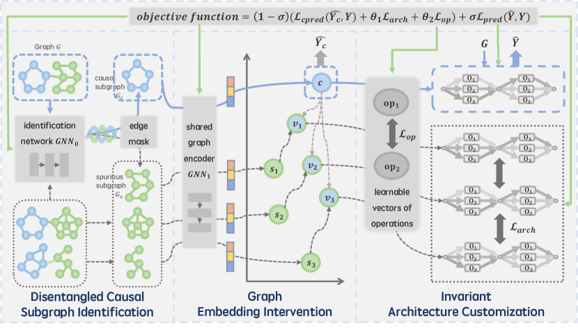
Figure 1: The framework of our proposed method CARNAS. As for an input graph $G$, the disentangled causal subgraph identification module abstracts its causal subgraph $G_{c}$ with disentangled GNN layers. Then, in the graph embedding intervention module, we conduct several interventions on $G_{c}$ with non-causal subgraphs in latent space and obtain $\mathcal{L}_{cpred}$ from the embedding of $G_{c}$ in the meanwhile. After that, the invariant architecture customization module aims to deal with distribution shift by customizing architecture from $G_{c}$ to attain $\hat{Y}$, $\mathcal{L}_{pred}$, and form $\mathcal{L}_{arch}$, $\mathcal{L}_{op}$ to further constrain the causal invariant property of $G_{c}$. Blue lines present the prediction approach and grey lines show other processes in the training stage. Additionally, green lines denote the updating process.

3 Method

We present our proposed method in this section based on the above causal view. Firstly, we present the disentangled causal subgraph identification module to obtain the causal subgraph for searching optimal architecture in Section 3.1. Then, we propose the intervention module in Section 3.2, to help with finding the invariant subgraph that is causally correlated with the optimal architectures, making the NAS model intrinsically interpretable to some degree. In Section 3.3, we introduce the simulated customization module which aims to deal with distribution shift by customizing for each graph and simulating the situation when the causal subgraph is affected by different spurious parts. Finally, we show the total invariant learning and optimization procedure in Section 3.4.

3.1 Disentangled Causal Subgraph Identification

This module utilizes disentangled GNN layers to capture different latent factors of the graph structure and further split the input graph instance $G$ into two subgraphs: causal subgraph $G_{c}$ and non-causal subgraph $G_{s}$. Specifically, considering an input graph $G=(\mathcal{V},\mathcal{E})$, its adjacency matrix is $\mathbf{D}\in\left\{0,1\right\}^{|\mathcal{V}|\times|\mathcal{V}|}$, where $\mathbf{D}_{i,j}=1$ denotes that there exists an edge between node $V_{i}$ and node $V_{j}$, while $\mathbf{D}_{i,j}=0$ otherwise. Since optimizing a discrete binary matrix $\mathbf{M}\in\left\{0,1\right\}^{|\mathcal{V}|\times|\mathcal{V}|}$ is unpractical due to the enormous number of subgraph candidates [50], and learning $\mathbf{M}$ separately for each input graph fails in generalizing to unseen test graphs [26], we adopt shared learnable disentangled GNN layers to comprehensively unveil the latent graph structural features and better abstract causal subgraphs. Firstly, we denote $Q$ as the number of latent features taken into account, and learn $Q$-chunk node representations by $Q$ GNNs:

$$\mathbf{Z}^{(l)}=\|_{q=1}^{Q}\operatorname{GNN_{0}}\left(\mathbf{Z}_{q}^{(l-1)},\mathbf{D}\right),$$ (4)

where $\mathbf{Z}_{q}^{l}$ is the $q$-th chunk of the node representation at $l$-th layer, $\mathbf{D}$ is the adjacency matrix, and $\|$ denotes concatenation. Then, we generate the edge importance scores $\mathcal{S}_{\mathcal{E}}\in\mathbb{R}^{|\mathcal{E}|\times 1}$ with an $\operatorname{MLP}$:

$$\mathcal{S}_{\mathcal{E}}=\operatorname{MLP}\left(\mathbf{Z}_{row}^{(L)},\mathbf{Z}_{col}^{(L)}\right),$$ (5)

where $\mathbf{Z}^{(L)}\in\mathbb{R}^{|\mathcal{V}|\times d}$ is the node representations after $L$ layers of disentangled GNN, and $\mathbf{Z}_{row}^{(L)},\mathbf{Z}_{col}^{(L)}$ are the subsets of $\mathbf{Z}^{(L)}$ containing the representations of row nodes and column nodes of edges $\mathcal{E}$ respectively. After that, we attain the causal and non-causal subgraphs by picking out the important edges through $\mathcal{S}_{\mathcal{E}}$:

$$\mathcal{E}_{c}=\operatorname{Top}_{t}(\mathcal{S}_{\mathcal{E}}),~{}\mathcal{E}_{s}=\mathcal{E}-\mathcal{E}_{c},$$ (6)

where $\mathcal{E}_{c}$ and $\mathcal{E}_{s}$ denotes the edge sets of $G_{c}$ and $G_{s}$, respectively, and $\operatorname{Top}_{t}(\cdot)$ selects the top $t$-percentage of edges with the largest edge score values.

3.2 Graph Embedding Intervention

After obtaining the causal subgraph $G_{c}$ and non-causal subgraph $G_{s}$ of an input graph $G$, we use another shared $\operatorname{GNN_{1}}$ to encode those subgraphs so as to do interventions in the same latent space:

$$\mathbf{Z_{c}}=\operatorname{GNN_{1}}\left(G_{c}\right),~{}\mathbf{Z_{s}}=\operatorname{GNN_{1}}\left(G_{s}\right).$$ (7)

Moreover, a readout layer is placed to aggregate node-level representations into graph-level representations:

$$\mathbf{H_{c}}=\operatorname{READOUT}\left(\mathbf{Z_{c}}\right),~{}\mathbf{H_{s}}=\operatorname{READOUT}\left(\mathbf{Z_{s}}\right).$$ (8)

3.2.1 Supervised classification for causal subgraphs

We claim that the causal subgraph $G_{c}$ inferred in Section 3.1 for finding the optimal GNN architecture is supposed to contain the main characteristic of graph $G$’s structure as well as capture the essential part for the final graph classification predicting task. Hence, we employ a classifier on $\mathbf{H_{c}}$ to construct a supervised classification loss:

$$\mathcal{L}_{cpred}=\sum_{i=1}^{N_{tr}}\ell\left(\hat{Y}_{c_{i}},Y_{i}\right),~{}\hat{Y}_{c_{i}}=\Phi\left({\mathbf{H_{c}}}_{i}\right),$$ (9)

where $\Phi$ is a classifier, $\hat{Y}_{c_{i}}$ is the prediction of graph $G_{i}$’s causal subgraph $G_{c_{i}}$ and $Y_{i}$ is the ground truth label of $G_{i}$.

3.2.2 Interventions by non-causal subgraphs

Based on subgraphs’ embedding $\mathbf{H_{c}}$ and $\mathbf{H_{s}}$, we formulate the intervened embedding $\mathbf{H_{v}}$ in the latent space. Specifically, we collect all the representations of non-causal subgraphs $\{{\mathbf{H_{s}}}_{i}\},i\in[1,N_{tr}]$, corresponding to each input graph $\{G_{i}\},i\in[1,N_{tr}]$, in the current batch, and randomly sample $N_{s}$ of them as the candidates $\{{\mathbf{H_{s}}}_{j}\},j\in[1,N_{s}]$ to do intervention with. As for a causal subgraph $G_{c}$ with representation $\mathbf{H_{c}}$, we define the representation under an intervention as:

$$do(S={G_{s}}_{j}):~{}\mathbf{H_{v}}_{j}=(1-\mu)\cdot{\mathbf{H_{c}}}+\mu\cdot{\mathbf{H_{s}}}_{j},~{}j\in[1,N_{s}],$$ (10)

in which $\mu\in(0,1)$ is the hyper-parameter to control the intensity of an intervention.

3.3 Invariant Architecture Customization

After obtaining graph representations $\mathbf{H_{c}}$ and ${{\mathbf{H_{v}}}}_{j},j\in[1,N_{s}]$, we introduce the method to construct a specific GNN architecture from a graph representation on the basis of differentiable NAS [24].

3.3.1 Architecture customization

To begin with, we denote the space of operator candidates as $\mathcal{O}$ and the number of architecture layers as $K$. Then, the ultimate architecture $A$ can be represented as a super-network:

$$g^{k}(\mathbf{x})=\sum_{u=1}^{|\mathcal{O}|}\alpha_{u}^{k}o_{u}(\mathbf{x}),~{}k\in[1,K],$$ (11)

where $\mathbf{x}$ is the input to layer $k$, $o_{u}(\cdot)$ is the operator from $\mathcal{O}$, $\alpha_{u}^{k}$ is the mixture coefficient of operator $o_{u}(\cdot)$ in layer $k$, and $g^{k}(x)$ is the output of layer $k$. Thereat, an architecture $A$ can be represented as a matrix $\mathbf{A}\in\mathbb{R}^{K\times|\mathcal{O}|}$, in which $\mathbf{A}_{k,u}=\alpha_{u}^{k}$. We learn these coefficients from graph representation $\mathbf{H}$ via trainable prototype vectors $\mathbf{op}_{u}^{k}~{}(u\in[1,|\mathcal{O}|],k\in[1,K])$, of operators:

$$\alpha_{u}^{k}=\frac{\exp\left({\mathbf{op}_{u}^{k}}^{T}\mathbf{H}\right)}{\sum_{u^{\prime}=1}^{|\mathcal{O}|}\exp\left({\mathbf{op}_{u^{\prime}}^{k}}^{T}\mathbf{H}\right)}.$$ (12)

In addition, the regularizer for operator prototype vectors:

$$\mathcal{L}_{op}=\sum_{k}\sum_{u,u^{\prime}\in[1,|\mathcal{O}|],u\neq u^{\prime}}\operatorname{cos}(\mathbf{op}_{u}^{k},\mathbf{op}_{u^{\prime}}^{k}),$$ (13)

where $\operatorname{cos}(\cdot,\cdot)$ is the cosine distance between two vectors, is engaged to avoid the mode collapse, following the exploration in [32].

3.3.2 Architectures from causal subgraph and intervention graphs

So far we form the mapping of $f_{A}:\mathbb{G}\rightarrow\mathcal{A}$ in Problem 2. As for an input graph $G$, we get its optimal architecture $A_{c}$ with the matrix $\mathbf{A_{c}}$ based on its causal subgraph’s representation $\mathbf{H_{c}}$ through equation (12), while for each intervention graph we have ${\mathbf{A_{v}}}_{j}$ based on ${\mathbf{H_{v}}}_{j},~{}j\in[1,N_{s}]$ similarly.

The customized architecture $A_{c}$ is used to produce the ultimate prediction of input graph $G$ by $f_{Y}:\mathbb{G}\times\mathcal{A}\rightarrow\mathbb{Y}$ in Problem 2, and we formulate the main classification loss as:

$$\mathcal{L}_{pred}=\sum_{i=1}^{N_{tr}}\ell(\hat{Y_{i}},Y_{i}),~{}\hat{Y_{i}}=f_{Y}(G_{i},{A_{c}}_{i}).$$ (14)

Furthermore, we regard each $\mathbf{A_{v}}_{j},~{}j\in[1,N_{s}]$ as an outcome when causal subgraph $G_{c}$ is in a specific environment (treating the intervened part, i.e. non-causal subgraphs, as different environments). Therefore, the following variance regularizer is proposed as a causal constraint to compel the inferred causal subgraph $G_{c}$ to have the steady ability to solely determine the optimal architecture for input graph instance $G$:

$$\mathcal{L}_{arch}=\frac{1}{N_{tr}}\sum_{i=1}^{N_{tr}}\mathbf{1}^{T}\cdot\mathbf{Var}_{i}\cdot\mathbf{1},\mathbf{Var}_{i}=\operatorname{var}\left(\left\{\mathbf{A_{v}}_{ij}\right\}\right),~{}j\in[1,N_{s}],$$ (15)

where $\operatorname{var}(\cdot)$ calculates the variance of a set of matrix, $\mathbf{1}^{T}\cdot\mathbf{Var}_{i}\cdot\mathbf{1}$ represents the summation of elements in matrix $\mathbf{Var}_{i}$.

3.4 Optimization Framework

Up to now, we have introduced $f_{C}:\mathbb{G}\xrightarrow{}\mathbb{G}_{c}$ in section 3.1, $f_{A}:\mathbb{G}_{c}\xrightarrow{}\mathcal{A}$ in section 3.2 and 3.3.1, $f_{Y}:\mathbb{G}\times\mathcal{A}\xrightarrow{}\mathbb{Y}$ in section 3.3.2, and whereby deal with Problem 2. To be specific, the overall objective function in equation (2) is as below:

$$\mathcal{L}_{all}=\sigma\mathcal{L}_{pred}+(1-\sigma)\mathcal{L}_{causal},\mathcal{L}_{causal}=\mathcal{L}_{cpred}+\theta_{1}\mathcal{L}_{arch}+\theta_{2}\mathcal{L}_{op},$$ (16)

where $\theta_{1}$, $\theta_{2}$ and $\sigma$ are hyper-parameters. Additionally, we adopt a linearly growing $\sigma_{p}$ corresponding to the epoch number $p$ as:

$$\sigma_{p}=\sigma_{min}+(p-1)\frac{\sigma_{max}-\sigma_{min}}{P},~{}p\in[1,P],$$ (17)

where $P$ is the maximum number of epochs. In this way, we can dynamically adjust the training key point in each epoch by focusing more on the causal-aware part (i.e. identifying suitable causal subgraph and learning vectors of operators) in the early stages and focusing more on the performance of the customized super-network in the later stages. We show the dynamic training process and how $\sigma_{p}$ improve the training and convergence efficiency in Appendix D.3. The overall framework and optimization procedure of the proposed CARNAS are summarized in Figure 1 and Algorithm 1.

4 Experiments

In this section, we present the comprehensive results of our experiments on both synthetic and real-world datasets to validate the effectiveness of our approach. We also conduct a series of ablation studies to thoroughly examine the contribution of the components within our framework. More analysis on experimental results, training efficiency, complexity and sensitivity are in Appendix D.

4.1 Experiment Setting

Setting.

To ensure reliability and reproducibility, we execute each experiment ten times using distinct random seeds and present the average results along with their standard deviations. We do not employ validation dataset for conducting architecture search. The configuration and use of datasets in our method align with those in other GNN methods, ensuring fairness across all approaches.

Baselines.

Table 1: The test accuracy of all methods on synthetic dataset Spurious-Motif. Values after $\pm$ denote the standard deviations. The best results overall are in bold and the best results of baselines in each category are underlined separately.

Method $b=0.7$ $b=0.8$ $b=0.9$ GCN $48.39_{\pm 1.69}$ $41.55_{\pm 3.88}$ $39.13_{\pm 1.76}$ GAT $50.75_{\pm 4.89}$ $42.48_{\pm 2.46}$ $40.10_{\pm 5.19}$ GIN $36.83_{\pm 5.49}$ $34.83_{\pm 3.10}$ $37.45_{\pm 3.59}$ SAGE $46.66_{\pm 2.51}$ $44.50_{\pm 5.79}$ $44.79_{\pm 4.83}$ GraphConv $47.29_{\pm 1.95}$ $44.67_{\pm 5.88}$ $44.82_{\pm 4.84}$ MLP $48.27_{\pm 1.27}$ $46.73_{\pm 3.48}$ $\underline{46.41_{\pm 2.34}}$ ASAP $\underline{54.07_{\pm 13.85}}$ $\underline{48.32_{\pm 12.72}}$ $43.52_{\pm 8.41}$ DIR $50.08_{\pm 3.46}$ $48.22_{\pm 6.27}$ $43.11_{\pm 5.43}$ Random $45.92_{\pm 4.29}$ $51.72_{\pm 5.38}$ $45.89_{\pm 5.09}$ DARTS $50.63_{\pm 8.90}$ $45.41_{\pm 7.71}$ $44.44_{\pm 4.42}$ GNAS $55.18_{\pm 18.62}$ $51.64_{\pm 19.22}$ $37.56_{\pm 5.43}$ PAS $52.15_{\pm 4.35}$ $43.12_{\pm 5.95}$ $39.84_{\pm 1.67}$ GRACES $65.72_{\pm 17.47}$ $59.57_{\pm 17.37}$ $50.94_{\pm 8.14}$ DCGAS $\underline{87.68_{\pm 6.12}}$ $\underline{75.45_{\pm 17.40}}$ $\underline{61.42_{\pm 16.26}}$ CARNAS $\textbf{94.41}_{\pm 4.58}$ $\textbf{88.04}_{\pm 13.77}$ $\textbf{87.15}_{\pm 11.85}$

We compare our model with 12 baselines from the following two different categories:

• Manually design GNNs. We incorporate widely recognized architectures GCN [17], GAT [38], GIN [46], SAGE [12], and GraphConv [28], and MLP into our search space as candidate operators as well as baseline methods in our experiments. Apart from that, we include two recent advancements: ASAP [33] and DIR [43], which is specifically proposed for out-of-distribution generalization.

• Graph Neural Architecture Search. For classic NAS, we compare with DARTS [24], a differentiable architecture search method, and random search. For graph NAS, we explore a reinforcement learning-based method GNAS [9], and PAS [39] that is specially designed for graph classification tasks. Additionally, we compare two state-of-the-art graph NAS methods that are specially designed for non-i.i.d. graph datasets, including GRACES [32] and DCGAS [48].

4.2 On Synthetic Datasets

Datasets.

The synthetic dataset, Spurious-Motif [32, 43, 50], encompasses 18,000 graphs, each uniquely formed by combining a base shape (denoted as Tree, Ladder, or Wheel with $S=0,1,2$) with a motif shape (represented as Cycle, House, or Crane with $C=0,1,2$). Notably, the classification of each graph relies solely on its motif shape, despite the base shape typically being larger. This dataset is particularly designed to study the effect of distribution shifts, with a distinct bias introduced solely on the training set through the probability distribution $P(S)=b\times\mathbb{I}(S=C)+\frac{1-b}{2}\times\mathbb{I}(S\neq C),$ where $b$ modulates the correlation between base and motif shapes, thereby inducing a deliberate shift between the training set and testing set, where all base and motif shapes are independent with equal probabilities. We choose $b=0.7/0.8/0.9$, enabling us to explore our model’s performance under various significant distributional variations. The effectiveness of our approach is measured using accuracy as the evaluation metric on this dataset.

Results.

Table 1 presents the experimental results on three synthetic datasets, revealing that our model significantly outperforms all baseline models across different scenarios.

Specifically, we observe that the performance of all GNN models is particularly poor, suggesting their sensitivity to spurious correlations and their inability to adapt to distribution shifts. However, DIR [43], designed specifically for non-I.I.D. datasets and focusing on discovering invariant rationale to enhance generalizability, shows pretty well performance compared to most of the other GNN models. This reflects the feasibility of employing causal learning to tackle generalization issues.

Moreover, NAS methods generally yield slightly better outcomes than manually designed GNNs in most scenarios, emphasizing the significance of automating architecture by learning the correlations between input graph data and architecture to search for the optimal GNN architecture. Notably, methods specifically designed for non-I.I.D. datasets, such as GRACES [32], DCGAS [48], and our CARNAS, exhibit significantly less susceptibility to distribution shifts compared to NAS methods intended for I.I.D. data.

Among these, our approach consistently achieves the best performance across datasets with various degrees of shifts, demonstrating the effectiveness of our method in enhancing Graph NAS performance, especially in terms of out-of-distribution generalization, which is attained by effectively capturing causal invariant subgraphs to guide the architecture search process, and filtering out spurious correlations meanwhile.

4.3 On Real-world Datasets

Table 2: The test ROC-AUC of all methods on real-world datasets OGBG-Mol*. Values after $\pm$ denote the standard deviations. The best results overall are in bold and the best results of baselines in each category are underlined separately.

Method	HIV	SIDER	BACE
GCN	$75.99_{\pm 1.19}$	$\underline{59.84_{\pm 1.54}}$	$68.93_{\pm 6.95}$
GAT	$76.80_{\pm 0.58}$	$57.40_{\pm 2.01}$	$75.34_{\pm 2.36}$
GIN	$\underline{77.07_{\pm 1.49}}$	$57.57_{\pm 1.56}$	$73.46_{\pm 5.24}$
SAGE	$75.58_{\pm 1.40}$	$56.36_{\pm 1.32}$	$74.85_{\pm 2.74}$
GraphConv	$74.46_{\pm 0.86}$	$56.09_{\pm 1.06}$	$\underline{78.87_{\pm 1.74}}$
MLP	$70.88_{\pm 0.83}$	$58.16_{\pm 1.41}$	$71.60_{\pm 2.30}$
ASAP	$73.81_{\pm 1.17}$	$55.77_{\pm 1.18}$	$71.55_{\pm 2.74}$
DIR	$77.05_{\pm 0.57}$	$57.34_{\pm 0.36}$	$76.03_{\pm 2.20}$
DARTS	$74.04_{\pm 1.75}$	$60.64_{\pm 1.37}$	$76.71_{\pm 1.83}$
PAS	$71.19_{\pm 2.28}$	$59.31_{\pm 1.48}$	$76.59_{\pm 1.87}$
GRACES	${77.31_{\pm 1.00}}$	${61.85_{\pm 2.58}}$	${79.46_{\pm 3.04}}$
DCGAS	$\underline{78.04_{\pm 0.71}}$	$\underline{63.46_{\pm 1.42}}$	$\underline{81.31_{\pm 1.94}}$
CARNAS	$\textbf{78.33}_{\pm 0.64}$	$\mathbf{83.36}_{\pm 0.62}$	$\textbf{81.73}_{\pm 2.92}$

Datasets.

The real-world datasets OGBG-Mol*, including Ogbg-molhiv, Ogbg-molbace, and Ogbg-molsider [13, 45], feature 41127, 1513, and 1427 molecule graphs, respectively, aimed at molecular property prediction. The division of the datasets is based on scaffold values, designed to segregate molecules according to their structural frameworks, thus introducing a significant challenge to the prediction of graph properties. The predictive performance of our approach across these diverse molecular structures and properties is measured using ROC-AUC as the evaluation metric.

Results.

Results from real-world datasets are detailed in Table 2, where our CARNAS model once again surpasses all baselines across three distinct datasets, showcasing its ability to handle complex distribution shifts under various conditions.

For manually designed GNNs, the optimal model varies across different datasets: GIN achieves the best performance on Ogbg-molhiv, GCN excels on Ogbg-molsider, and GraphConv leads on Ogbg-molbace. This diversity in performance confirms a crucial hypothesis in our work, that different GNN models are predisposed to perform well on graphs featuring distinct characteristics.

In the realm of NAS models, we observe that DARTS and PAS, proposed for I.I.D. datasets, perform comparably to manually crafted GNNs, whereas GRACES, DCGAS and our CARNAS, specifically designed for non-I.I.D. datasets outshine other baselines. Our approach reaches the top performance across all datasets, with a particularly remarkable breakthrough on Ogbg-molsider, highlighting our method’s superior capability in adapting to and excelling within diverse data environments.

4.4 Ablation Study

In this section, we conduct ablation studies to examine the effectiveness of each vital component in our framework. Detailed settings are in Appendix C.3.1.

Results.

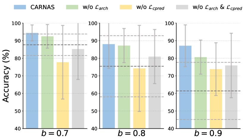
Figure 2: Results of ablation studies on synthetic datasets, where ‘w/o $\mathcal{L}_{arch}$’ removes $\mathcal{L}_{arch}$ from the overall loss in Eq. (16), ‘w/o $\mathcal{L}_{cpred}$’ removes $\mathcal{L}_{cpred}$, and ‘w/o $\mathcal{L}_{arch}$ & $\mathcal{L}_{cpred}$’ removes both of them. The error bars report the standard deviations. Besides, the average and standard deviations of the best-performed baseline on each dataset are denoted as the dark and light thick dash lines respectively.

From Figure 2, we have the following observations. First of all, our proposed CARNAS outperforms all the variants as well as the best-performed baseline on all datasets, demonstrating the effectiveness of each component of our proposed method. Secondly, the performance of ‘CARNAS w/o $\mathcal{L}_{arch}$’, ‘CARNAS w/o $\mathcal{L}_{cpred}$’ and ‘CARNAS w/o $\mathcal{L}_{arch}$ & $\mathcal{L}_{cpred}$’ dropped obviously on all datasets comparing with the full CARNAS , which validates that our proposed modules help the model to identify stable causal components from comprehensive graph feature and further guide the Graph NAS process to enhance its performance significantly especially under distribution shifts. What’s more, though ‘CARNAS w/o $\mathcal{L}_{arch}$’ decreases, its performance still surpasses the best results in baselines across all datasets, indicating that even if the invariance of the influence of the causal subgraph on the architecture is not strictly restricted by $\mathcal{L}_{arch}$, it is effective to use merely the causal subgraph guaranteed by $\mathcal{L}_{cpred}$ to contain the important information of the input graph and use it to guide the architecture search.

5 Related Work

Neural Architecture Search (NAS) automates creating optimal neural networks using RL-based [57], evolutionary [34], and gradient-based methods [24]. GraphNAS [9] inspired studies on GNN architectures for graph classification in various datasets [32, 48]. Real-world data differences between training and testing sets impact GNN performance [35, 20, 52, 53]. Studies [21, 8] identify invariant subgraphs to mitigate this, usually with fixed GNN encoders. Our method automates designing generalized graph architectures by discovering causal relationships. Causal learning explores variable interconnections [31], enhancing deep learning [51]. In graphs, it includes interventions on non-causal components [44], causal and bias subgraph decomposition [8], and ensuring out-of-distribution generalization [6, 54, 55]. These methods use fixed GNN architectures, while we address distribution shifts by discovering causal relationships between graphs and architectures.

6 Conclusion

In this paper, we address distribution shifts in graph neural architecture search (Graph NAS) from a causal perspective. Existing methods struggle with distribution shifts between training and testing sets due to spurious correlations. To mitigate this, we introduce Causal-aware Graph Neural Architecture Search (CARNAS). Our approach identifies stable causal structures and their relationships with architectures. We propose three key modules: Disentangled Causal Subgraph Identification, Graph Embedding Intervention, and Invariant Architecture Customization. These modules leverage causal relationships to search for generalized graph neural architectures. Experiments on synthetic and real-world datasets show that CARNAS achieves superior out-of-distribution generalization, highlighting the importance of causal awareness in Graph NAS.

Appendix A Notation

Table 3: Important Notation

Notation	Meaning
$\mathbb{G}$, $\mathbb{Y}$	Graph space and Label space
$\mathcal{G}_{tr}$, $\mathcal{G}_{te}$	Training graph dataset, Testing graph dataset
$G_{i}$, $Y_{i}$	Graph instance $i$, Label of graph instance $i$
$G_{c}$, $G_{s}$	Causal subgraph and Non-causal subgraph
$\mathbf{D}$	Adjacency matrix of graph $G$
$\mathbf{Z}$	Node representations
$\mathcal{S}_{\mathcal{E}}$	Edge importance scores
$\mathcal{E}_{c}$, $\mathcal{E}_{s}$	Edge set of the causal subgraph and the non-causal subgraph
$\mathbf{H_{c}}$, $\mathbf{H_{s}}$	Graph-level representation of causal subgraph and non-causal subgraph
$\hat{Y}_{c_{i}}$	Prediction of graph $G_{i}$’s causal subgraph $G_{c_{i}}$
$\mathbf{H_{v}}$	Intervened graph representation
$\mathcal{O}$, $o_{u}(\cdot)$	Space of operator candidates, operator from $\mathcal{O}$
$K$	Number of architecture layers
$\mathcal{A}$	Search space of GNN architectures
$A$, $\mathbf{A}$	An architecture represented as a super-network; matrix of architecture A
$g^{k}(\mathbf{x})$	Output of layer $k$ in the architecture.
$\alpha_{u}^{k}$	Mixture coefficient of operator $o_{u}(\cdot)$ in layer $k$
$\mathbf{op}_{u}^{k}$	Trainable prototype vectors of operators

Appendix B Algorithm

The overall framework and optimization procedure of the proposed CARNAS are summarized in Figure 1 and Algorithm 1, respectively.

Algorithm 1 The overall algorithm of CARNAS

0:  Training Dataset $\mathcal{G}_{tr}$, Hyper-parameters $t$ in Eq. (6), $\mu$ in Eq. (10), $\theta_{1}$, $\theta_{2}$ in Eq. (16)

1:  Initialize all trainable parameters

2:  for $p=1,\ldots,P$ do

3:     Set $\sigma_{p}$ as Eq. (17)

4:     Derive causal and non-causal subgraphs as Eq. (4) (5) (6)

5:     Calculate graph representations of causal and non-causal subgraphs as Eq. (7) (8)

6:     Calculate $\mathcal{L}_{cpred}$ using Eq. (9)

7:     Sample $N_{s}$ non-causal subgraphs as candidates

8:     for causal subgraph $G_{c}$ of graph $G$ in $\mathcal{G}_{tr}$ do

9:        Do interventions on $G_{c}$ in latent space as Eq. (10)

10:        Calculate architecture matrix $\mathbf{A_{c}}$ and $\{\mathbf{A_{v}}_{j}\}$ from causal subgraph and their intervention graphs as Eq. (12)

11:     end for

12:     Calculate $\mathcal{L}_{op}$ using Eq. (13)

13:     Calculate $\mathcal{L}_{pred}$ using Eq. (11) (14)

14:     Calculate $\mathcal{L}_{arch}$ using Eq. (15))

15:     Calculate the overall loss $\mathcal{L}_{all}$ using Eq. (16)

16:     Update parameters using gradient descends

17:  end for

Appendix C Reproducibility Details

C.1 Definition of Search Space

The number of layers in our model is predetermined before training, and the type of operator for each layer can be selected from our defined operator search space $\mathcal{O}$. We incorporate widely recognized architectures GCN, GAT, GIN, SAGE, GraphConv, and MLP into our search space as candidate operators in our experiments. This allows for the combination of various sub-architectures within a single model, such as using GCN in the first layer and GAT in the second layer. Furthermore, we consistently use standard global mean pooling at the end of the GNN architecture to generate a global embedding.

C.2 Datasets Details

We utilize synthetic SPMotif datasets, which are characterized by three distinct degrees of distribution shifts, and three different real-world datasets, each with varied components, following previous works [32, 48, 43]. Based on the statistics of each dataset as shown in Table 4, we conducted a comprehensive comparison across various scales and graph sizes. This approach has empirically validated the scalability of our model.

Table 4: Statistics for different datasets.

	Graphs	Avg. Nodes	Avg. Edges
ogbg-molhiv	41127	25.5	27.5
ogbg-molsider	1427	33.6	35.4
ogbg-molbace	1513	34.1	36.9
SPMotif-0.7/0.8/0.9	18000	26.1	36.3

Detailed description for real-world datasets

The real-world datasets are 3 molecular property prediction datasets in OGB [13], and are adopted from the MoleculeNet [45]. Each graph represents a molecule, where nodes are atoms, and edges are chemical bonds.

• The HIV dataset was introduced by the Drug Therapeutics Program (DTP) AIDS Antiviral Screen, which tested the ability to inhibit HIV replication for over 40000 compounds. Screening results were evaluated and placed into 2 categories: inactive (confirmed inactive CI) and active (confirmed active CA and confirmed moderately active CM).

• The Side Effect Resource (SIDER) is a database of marketed drugs and adverse drug reactions (ADR). The version of the SIDER dataset in DeepChem has grouped drug side-effects into 27 system organ classes following MedDRA classifications measured for 1427 approved drugs (following previous usage).

• The BACE dataset provides quantitative ($IC_{50}$) and qualitative (binary label) binding results for a set of inhibitors of human $\beta$-secretase 1 (BACE-1). It merged a collection of 1522 compounds with their 2D structures and binary labels in MoleculeNet, built as a classification task.

The division of the datasets is based on scaffold values, designed to segregate molecules according to their structural frameworks, thus introducing a significant challenge to the prediction of graph properties.

C.3 Detailed Hyper-parameter Settings

We fix the number of latent features $Q=4$ in Eq. (4), number of intervention candidates $N_{s}$ as batch size in Eq. (10), $\sigma_{min}=0.1$, $\sigma_{max}=0.7$, $P=100$ in Eq. (17), and the tuned hyper-parameters for each dataset are as in Table 5.

Table 5: Hyper-parameter settings

Dataset	$t$ in Eq. (6)	$\mu$ in Eq. (10)	$\theta_{1}$ in Eq. (16)	$\theta_{2}$ in Eq. (16)
SPMotif-0.7/0.8/0.9	0.85	0.26	0.36	0.010
ogbg-molhiv	0.46	0.68	0.94	0.007
ogbg-molsider	0.40	0.60	0.85	0.005
ogbg-molbace	0.49	0.54	0.80	0.003

C.3.1 Detailed Settings for Ablation Study

We compare the following ablated variants of our model in Section 4.4:

• ‘CARNAS w/o $\mathcal{L}_{arch}$’ removes $\mathcal{L}_{arch}$ from the overall loss in Eq. (16). In this way, the contribution of the graph embedding intervention module together with the invariant architecture customization module to improve generalization performance by restricting the causally invariant nature for constructing architectures of the causal subgraph is removed.

• ‘CARNAS w/o $\mathcal{L}_{cpred}$’ removes $\mathcal{L}_{cpred}$, thereby relieving the supervised restriction on causal subgraphs for encapsulating sufficient graph features, which is contributed by disentangled causal subgraph identification module together with the graph embedding intervention module to enhance the learning of causal subgraphs.

• ‘CARNAS w/o $\mathcal{L}_{arch}$ & $\mathcal{L}_{cpred}$’ further removes both of them.

Appendix D Deeper Analysis

D.1 Supplementary Analysis of the Experimental Results

Sythetic datasets.

We notice that the performance of CARNAS is way better than DIR [43], which also introduces causality in their method, on synthetic datasets. We provide an explanation as follows: Our approach differs from and enhances upon DIR in several key points. Firstly, unlike DIR, which uses normal GNN layers for embedding nodes and edges to derive a causal subgraph, we employ disentangled GNN. This allows for more effective capture of latent features when extracting causal subgraphs. Secondly, while DIR focuses on the causal relationship between a graph instance and its label, our study delves into the causal relationship between a graph instance and its optimal architecture, subsequently using this architecture to predict the label. Additionally, we incorporate NAS method, introducing an invariant architecture customization module, which considers the impact of architecture on performance. Based on these advancements, our method may outperform DIR.

Figure 3: Results of ablation studies on SIDER, where ‘w/o $\mathcal{L}_{arch}$’ removes $\mathcal{L}_{arch}$ from the overall loss in Eq. (16), ‘w/o $\mathcal{L}_{cpred}$’ removes $\mathcal{L}_{cpred}$, and ‘w/o $\mathcal{L}_{arch}$ & $\mathcal{L}_{cpred}$’ removes both of them. The error bars report the standard deviations. Besides, the average and standard deviations of the best-performed baseline on each dataset are denoted as the dark and light thick dash lines respectively.

Real-world datasets.

We also notice that our methods improves a lot on the performance for the second real-world dataset SIDER. We further conduct an ablation study on SIDER to confirm that each proposed component contributes to its performance, as present in Figure 3. The model ‘w/o $L{arch}$’ shows a slight decrease in performance, while ‘w/o $L{cpred}$’ exhibits a substantial decline. This indicates that both restricting the invariance of the influence of the causal subgraph on the architecture via $L{arch}$, and ensuring that the causal subgraph retains crucial information from the input graph via $L{cpred}$, are vital for achieving high performance on SIDER, especially the latter which empirically proves to be exceptionally effective.

D.2 Complexity Analysis

In this section, we analyze the complexity of our proposed method in terms of its computational time and the quantity of parameters that require optimization. Let’s denote by $|V|$ the number of nodes in a graph, by $|E|$ the number of edges, by $|\mathcal{O}|$ the size of search space, and by $d$ the dimension of hidden representations within a traditional graph neural network (GNN) framework. In our approach, $d_{0}$ represents the dimension of the hidden representations within the identification network $\operatorname{GNN_{0}}$, $d_{1}$ represents the dimension of the hidden representations within the shared graph encoder $\operatorname{GNN_{1}}$, and $d_{s}$ denotes the dimension within the tailored super-network. Notably, $d_{0}$ encapsulates the combined dimension of $Q$ chunks, meaning the dimension per chunk is $d_{0}/Q$.

D.2.1 Time complexity analysis

For most message-passing GNNs, the computational time complexity is traditionally $O(|E|d+|V|d^{2})$. Following this framework, the $\operatorname{GNN_{0}}$ in our model exhibits a time complexity of $O(|E|d_{0}+|V|d_{0}^{2})$, and the $\operatorname{GNN_{1}}$ in our model exhibits a time complexity of $O(|E|d_{1}+|V|d_{1}^{2})$. The most computationally intensive operation in the invariant architecture customization module, which involves the computation of $\mathcal{L}_{op}$, leads to a time complexity of $O(|\mathcal{O}|^{2}d_{1})$. The time complexity attributed to the customized super-network is $O(|\mathcal{O}|(|E|d_{s}+|V|d_{s}^{2}))$. Consequently, the aggregate time complexity of our method can be summarized as $O(|E|(d_{0}+d_{1}+|\mathcal{O}|d_{s})+|V|(d_{0}^{2}+d_{1}^{2}+|\mathcal{O}|d_{s}^{2})+|\mathcal{O}|^{2}d_{1})$.

D.2.2 Parameter complexity analysis

A typical message-passing GNN has a parameter complexity of $O(d^{2})$. In our architecture, the disentangled causal subgraph identification network $\operatorname{GNN_{0}}$ possesses $O(d_{0}^{2})$ parameters, the shared GNN encoder $\operatorname{GNN_{1}}$ possesses $O(d_{1}^{2})$, the invariant architecture customization module contains $O(|\mathcal{O}|d_{1})$ parameters and the customized super-network is characterized by $O(|\mathcal{O}|d_{s}^{2})$ parameters. Therefore, the total parameter complexity in our framework is expressed as $O(d_{0}^{2}+d_{1}^{2}+|\mathcal{O}|d_{1}+|\mathcal{O}|d_{s}^{2})$.

The analyses underscore that the proposed method scales linearly with the number of nodes and edges in the graph and maintains a constant number of learnable parameters, aligning it with the efficiency of prior GNN and graph NAS methodologies. Moreover, given that $|\mathcal{O}|$ typically represents a modest constant (for example, $|\mathcal{O}|=6$ in our search space) and that $d_{0}$ and $d_{1}$ is generally much less than $d_{s}$, the computational and parameter complexities are predominantly influenced by $d_{s}$. To ensure equitable comparisons with existing GNN baselines, we calibrate $d_{s}$ within our model such that the parameter count, specifically $|\mathcal{O}|d_{s}^{2}$, approximates $d^{2}$, thereby achieving a balance between efficiency and performance.

D.3 Dynamic Training Process and Convergence

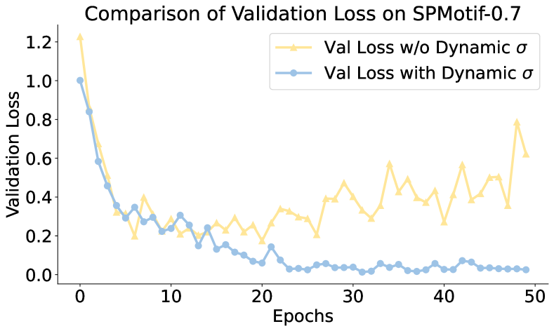
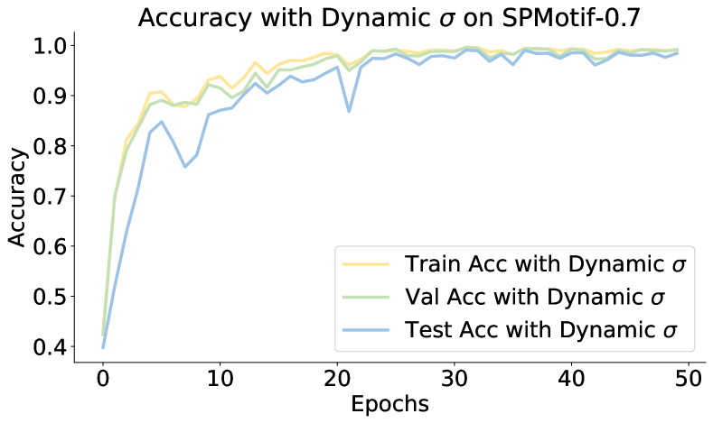
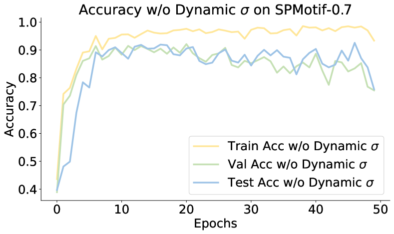
Figure 4: Training process of synthetic datasets.

For a deeper understanding of our model training process, and further remark the impact of the dynamic $\sigma_{p}$ in Eq.(17), we conduct experiments and compare the training process in the following settings:

• ‘with Dynamic $\sigma$’ means we use the dynamic $\sigma_{p}$ in Eq.(17) to adjust the training key point in each epoch.

• ‘w/o Dynamic $\sigma$’ means we fix the $\sigma$ in Eq.(16) as a constant value $\frac{\sigma_{max}+\sigma_{min}}{2}$.

According to Figure 4, our method can converge rapidly in 10 epochs. Figure 4 also obviously reflects that after 10 epochs the validation loss with dynamic $\sigma$ keeps declining and its accuracy continuously rising. However, in the setting without dynamic $\sigma$, the validation loss may rise again, and accuracy cannot continue to improve.

These results verify our aim to adopt this $\sigma_{p}$ to elevate the efficiency of model training in the way of dynamically adjusting the training key point in each epoch by focusing more on the causal-aware part (i.e. identifying suitable causal subgraph and learning vectors of operators) in the early stages and focusing more on the performance of the customized super-network in the later stages. We also empirically confirm that our method is not complex to train.

D.4 Training Efficiency

To further illustrate the efficiency of CARNAS, we provide a direct comparison with the best-performed NAS baseline, DCGAS, based on the total runtime for 100 epochs. As shown in Table 6, CARNAS consistently requires less time across different datasets while achieving superior best performance, demonstrating its enhanced efficiency and effectiveness.

Table 6: Comparison of runtime

Method	SPMotif	HIV	BACE	SIDER
DCGAS	104 min	270 min	12 min	11 min
CARNAS	76 min	220 min	8 min	8 min

D.5 Hyper-parameters Sensitivity

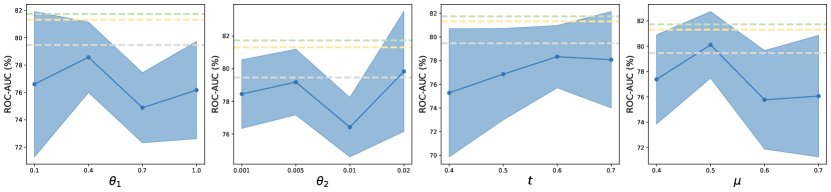
Figure 5: Hyper-parameters sensitivity analysis. The area shows the average ROC-AUC and standard deviations. The green, yellow, grey dashed lines represent the average performance corresponding to the fine-tuned hyper-parameters of CARNAS, best performed baseline DCGAS, 2nd best performed baseline GRACES, respectively.

We empirically observe that our model is insensitive to most hyper-parameters, which remain fixed throughout our experiments. Consequently, the number of parameters requiring tuning in practice is relatively small. $t$, $\mu$, $\theta_{1}$ and $\theta_{2}$ have shown more sensitivity, prompting us to focus our tuning efforts on these 4 hyper-parameters.

Therefore, we conduct sensitivity analysis (on BACE) for the 4 important hyper-parameters, as shown in Figure 5. The value selection for these parameters were deliberately varied evenly within a defined range to assess sensitivity thoroughly. The specific hyper-parameter settings used for the CARNAS reported in Table 2 are more finely tuned and demonstrate superior performance to the also finely tuned other baselines. The sensitivity allows for potential performance improvements through careful parameter tuning, and our results in sensitivity analysis outperform most baseline methods, indicating a degree of stability and robustness in response to these hyper-parameters.

Mention that, the best performance of the fine-tuned DCGAS may exceed the performance of our method without fine-tuning sometimes. This is because, DCGAS addresses the challenge of out-of-distribution generalization through data augmentation, generating a sufficient quantity of graphs for training. In contrast, CARNAS focuses on capturing and utilizing causal and stable subparts to guide the architecture search process. The methodological differences and the resulting disparity in the volume of data used could also contribute to the performance variations observed.

Limitation.

Although the training time and search efficiency of our method is comparable to most of the Graph NAS methods, we admit that it is less efficient than standard GNNs. At the same time, in order to obtain the best performance for a certain application scenario, our method does need to fine-tune four sensitive hyper-parameters.

Appendix E Related Work

E.1 Graph Neural Architecture Search

In the rapidly evolving domain of automatic machine learning, Neural Architecture Search (NAS) represents a groundbreaking shift towards automating the discovery of optimal neural network architectures. This shift is significant, moving away from the traditional approach that heavily relies on manual expertise to craft models. NAS stands out by its capacity to autonomously identify architectures that are finely tuned for specific tasks, demonstrating superior performance over manually engineered counterparts. The exploration of NAS has led to the development of diverse strategies, including reinforcement learning (RL)-based approaches [57, 14], evolutionary algorithms-based techniques [34, 25], and methods that leverage gradient information [24, 49]. Among these, graph neural architecture search has garnered considerable attention.

The pioneering work of GraphNAS [9] introduced the use of RL for navigating the search space of graph neural network (GNN) architectures, incorporating successful designs from the GNN literature such as GCN, GAT, etc. This initiative has sparked a wave of research [9, 39, 32, 4, 11, 56, 10], leading to the discovery of innovative and effective architectures. Recent years have seen a broadening of focus within Graph NAS towards tackling graph classification tasks, which are particularly relevant for datasets comprised of graphs, such as those found in protein molecule studies. This research area has been enriched by investigations into graph classification on datasets that are either independently identically distributed [39] or non-independently identically distributed, with GRACES [32] and DCGAS [48] being notable examples of the latter. Through these efforts, the field of NAS continues to expand its impact, offering tailored solutions across a wide range of applications and datasets.

E.2 Graph Out-of-Distribution Generalization

In the realm of machine learning, a pervasive assumption posits the existence of identical distributions between training and testing data. However, real-world scenarios frequently challenge this assumption with inevitable shifts in distribution, presenting significant hurdles to model performance in out-of-distribution (OOD) scenarios [35, 52, 53]. The drastic deterioration in performance becomes evident when models lack robust OOD generalization capabilities, a concern particularly pertinent in the domain of Graph Neural Networks (GNNs), which have gained prominence within the graph community [20]. Several noteworthy studies [42, 41, 21, 8, 36, 23, 37] have tackled this challenge by focusing on identifying environment-invariant subgraphs to mitigate distribution shifts. These approaches typically rely on pre-defined or dynamically generated environment labels from various training scenarios to discern variant information and facilitate the learning of invariant subgraphs. Moreover, the existing methods usually adopt a fixed GNN encoder in the whole optimization process, neglecting the role of graph architectures in out-of-distribution generalization. In this paper, we focus on automating the design of generalized graph architectures by discovering causal relationships between graphs and architectures, and thus handle distribution shifts on graphs.

E.3 Causal Learning on Graphs

The field of causal learning investigates the intricate connections between variables [31, 29], offering profound insights that have significantly enhanced deep learning methodologies. Leveraging causal relationships, numerous techniques have made remarkable strides across diverse computer vision applications  [51, 27]. Additionally, recent research has delved into the realm of graphs [54, 55]. For instance,  [44] implements interventions on non-causal components to generate representations, facilitating the discovery of underlying graph rationales.  [8] decomposes graphs into causal and bias subgraphs, mitigating dataset biases.  [22] introduces invariance into self-supervised learning, preserving stable semantic information.  [6] ensures out-of-distribution generalization by capturing graph invariance.  [15] tackled the challenge of learning causal graphs involving latent variables, which are derived from a mixture of observational and interventional distributions with unknown interventional objectives. To mitigate this issue, the study proposed an approach leveraging a $\Psi$-Markov property.  [1] introduced a randomized algorithm, featuring $p$-colliders, for recovering the complete causal graph while minimizing intervention costs. Additionally,  [3] presented an adaptable method for causality detection, which notably benefits from various types of interventional data and incorporates sophisticated neural architectures such as normalizing flows, operating under continuous constraints. However, these methods adopt a fixed GNN architecture in the optimization process, neglecting the role of architectures in causal learning on graphs. In contrast, in this paper, we focus on handling distribution shifts in the graph architecture search process from the causal perspective by discovering the causal relationship between graphs and architectures.

References

- [1] Raghavendra Addanki, Shiva Kasiviswanathan, Andrew McGregor, and Cameron Musco. Efficient intervention design for causal discovery with latents. In International Conference on Machine Learning, pages 63–73. PMLR, 2020.
- [2] Martin Arjovsky, Léon Bottou, Ishaan Gulrajani, and David Lopez-Paz. Invariant risk minimization. arXiv preprint arXiv:1907.02893, 2019.
- [3] Philippe Brouillard, Sébastien Lachapelle, Alexandre Lacoste, Simon Lacoste-Julien, and Alexandre Drouin. Differentiable causal discovery from interventional data. Advances in Neural Information Processing Systems, 33:21865–21877, 2020.
- [4] Shaofei Cai, Liang Li, Jincan Deng, Beichen Zhang, Zheng-Jun Zha, Li Su, and Qingming Huang. Rethinking graph neural architecture search from message-passing. In Proceedings of the IEEE/CVF Conference on Computer Vision and Pattern Recognition, pages 6657–6666, 2021.
- [5] Shiyu Chang, Yang Zhang, Mo Yu, and Tommi Jaakkola. Invariant rationalization. In International Conference on Machine Learning, pages 1448–1458. PMLR, 2020.
- [6] Yongqiang Chen, Yonggang Zhang, Yatao Bian, Han Yang, MA Kaili, Binghui Xie, Tongliang Liu, Bo Han, and James Cheng. Learning causally invariant representations for out-of-distribution generalization on graphs. Advances in Neural Information Processing Systems, 35:22131–22148, 2022.
- [7] Gabriele Corso, Luca Cavalleri, Dominique Beaini, Pietro Liò, and Petar Veličković. Principal neighbourhood aggregation for graph nets. Advances in Neural Information Processing Systems, 33:13260–13271, 2020.
- [8] Shaohua Fan, Xiao Wang, Yanhu Mo, Chuan Shi, and Jian Tang. Debiasing graph neural networks via learning disentangled causal substructure. In NeurIPS, 2022.
- [9] Yang Gao, Hong Yang, Peng Zhang, Chuan Zhou, and Yue Hu. Graph neural architecture search. In International joint conference on artificial intelligence. International Joint Conference on Artificial Intelligence, 2021.
- [10] Chaoyu Guan, Xin Wang, Hong Chen, Ziwei Zhang, and Wenwu Zhu. Large-scale graph neural architecture search. In International Conference on Machine Learning, pages 7968–7981. PMLR, 2022.
- [11] Chaoyu Guan, Xin Wang, and Wenwu Zhu. Autoattend: Automated attention representation search. In International conference on machine learning, pages 3864–3874. PMLR, 2021.
- [12] Will Hamilton, Zhitao Ying, and Jure Leskovec. Inductive representation learning on large graphs. Advances in neural information processing systems, 30, 2017.
- [13] Weihua Hu, Matthias Fey, Marinka Zitnik, Yuxiao Dong, Hongyu Ren, Bowen Liu, Michele Catasta, and Jure Leskovec. Open graph benchmark: Datasets for machine learning on graphs. Advances in neural information processing systems, 33:22118–22133, 2020.
- [14] Yesmina Jaafra, Jean Luc Laurent, Aline Deruyver, and Mohamed Saber Naceur. Reinforcement learning for neural architecture search: A review. Image and Vision Computing, 89:57–66, 2019.
- [15] Amin Jaber, Murat Kocaoglu, Karthikeyan Shanmugam, and Elias Bareinboim. Causal discovery from soft interventions with unknown targets: Characterization and learning. Advances in neural information processing systems, 33:9551–9561, 2020.
- [16] Yuanfeng Ji, Lu Zhang, Jiaxiang Wu, Bingzhe Wu, Long-Kai Huang, Tingyang Xu, Yu Rong, Lanqing Li, Jie Ren, Ding Xue, et al. Drugood: Out-of-distribution (ood) dataset curator and benchmark for ai-aided drug discovery–a focus on affinity prediction problems with noise annotations. arXiv preprint arXiv:2201.09637, 2022.
- [17] Thomas N Kipf and Max Welling. Semi-supervised classification with graph convolutional networks. In International Conference on Learning Representations, 2016.
- [18] David Krueger, Ethan Caballero, Joern-Henrik Jacobsen, Amy Zhang, Jonathan Binas, Dinghuai Zhang, Remi Le Priol, and Aaron Courville. Out-of-distribution generalization via risk extrapolation (rex). In International Conference on Machine Learning, pages 5815–5826. PMLR, 2021.
- [19] Guohao Li, Guocheng Qian, Itzel C Delgadillo, Matthias Muller, Ali Thabet, and Bernard Ghanem. Sgas: Sequential greedy architecture search. In Proceedings of the IEEE/CVF Conference on Computer Vision and Pattern Recognition, pages 1620–1630, 2020.
- [20] Haoyang Li, Xin Wang, Ziwei Zhang, and Wenwu Zhu. Out-of-distribution generalization on graphs: A survey. arXiv preprint arXiv:2202.07987, 2022.
- [21] Haoyang Li, Ziwei Zhang, Xin Wang, and Wenwu Zhu. Learning invariant graph representations for out-of-distribution generalization. Advances in Neural Information Processing Systems, 35:11828–11841, 2022.
- [22] Sihang Li, Xiang Wang, An Zhang, Yingxin Wu, Xiangnan He, and Tat-Seng Chua. Let invariant rationale discovery inspire graph contrastive learning. In ICML, pages 13052–13065, 2022.
- [23] Gang Liu, Tong Zhao, Jiaxin Xu, Tengfei Luo, and Meng Jiang. Graph rationalization with environment-based augmentations. In Proceedings of the 28th ACM SIGKDD International Conference on Knowledge Discovery & Data Mining, 2022.
- [24] Hanxiao Liu, Karen Simonyan, and Yiming Yang. Darts: Differentiable architecture search. In International Conference on Learning Representations, 2018.
- [25] Yuqiao Liu, Yanan Sun, Bing Xue, Mengjie Zhang, Gary G Yen, and Kay Chen Tan. A survey on evolutionary neural architecture search. IEEE transactions on neural networks and learning systems, 2021.
- [26] Dongsheng Luo, Wei Cheng, Dongkuan Xu, Wenchao Yu, Bo Zong, Haifeng Chen, and Xiang Zhang. Parameterized explainer for graph neural network. Advances in neural information processing systems, 33:19620–19631, 2020.
- [27] Jovana Mitrovic, Brian McWilliams, Jacob C Walker, Lars Holger Buesing, and Charles Blundell. Representation learning via invariant causal mechanisms. In ICLR, 2020.
- [28] Christopher Morris, Martin Ritzert, Matthias Fey, William L Hamilton, Jan Eric Lenssen, Gaurav Rattan, and Martin Grohe. Weisfeiler and leman go neural: Higher-order graph neural networks. In Proceedings of the AAAI conference on artificial intelligence, volume 33, pages 4602–4609, 2019.
- [29] Judea Pearl. Causality. Cambridge university press, 2009.
- [30] Judea Pearl et al. Models, reasoning and inference. Cambridge, UK: CambridgeUniversityPress, 19(2):3, 2000.
- [31] Judea Pearl, Madelyn Glymour, and Nicholas P Jewell. Causal inference in statistics: A primer. John Wiley & Sons, 2016.
- [32] Yijian Qin, Xin Wang, Ziwei Zhang, Pengtao Xie, and Wenwu Zhu. Graph neural architecture search under distribution shifts. In International Conference on Machine Learning, pages 18083–18095. PMLR, 2022.
- [33] Ekagra Ranjan, Soumya Sanyal, and Partha Talukdar. Asap: Adaptive structure aware pooling for learning hierarchical graph representations. In Proceedings of the AAAI Conference on Artificial Intelligence, volume 34, pages 5470–5477, 2020.
- [34] Esteban Real, Sherry Moore, Andrew Selle, Saurabh Saxena, Yutaka Leon Suematsu, Jie Tan, Quoc V Le, and Alexey Kurakin. Large-scale evolution of image classifiers. In International conference on machine learning, pages 2902–2911. PMLR, 2017.
- [35] Zheyan Shen, Jiashuo Liu, Yue He, Xingxuan Zhang, Renzhe Xu, Han Yu, and Peng Cui. Towards out-of-distribution generalization: A survey. arXiv:2108.13624, 2021.
- [36] Yongduo Sui, Xiang Wang, Jiancan Wu, Min Lin, Xiangnan He, and Tat-Seng Chua. Causal attention for interpretable and generalizable graph classification. Proceedings of the 28th ACM SIGKDD International Conference on Knowledge Discovery & Data Mining, 2022.
- [37] Yongduo Sui, Qitian Wu, Jiancan Wu, Qing Cui, Longfei Li, Jun Zhou, Xiang Wang, and Xiangnan He. Unleashing the power of graph data augmentation on covariate distribution shift. In Thirty-seventh Conference on Neural Information Processing Systems, 2023.
- [38] Petar Velickovic, Guillem Cucurull, Arantxa Casanova, Adriana Romero, Pietro Lio, Yoshua Bengio, et al. Graph attention networks. stat, 1050(20):10–48550, 2017.
- [39] Lanning Wei, Huan Zhao, Quanming Yao, and Zhiqiang He. Pooling architecture search for graph classification. In Proceedings of the 30th ACM International Conference on Information & Knowledge Management, pages 2091–2100, 2021.
- [40] Qitian Wu, Hengrui Zhang, Junchi Yan, and David Wipf. Handling distribution shifts on graphs: An invariance perspective. In International Conference on Learning Representations, 2021.
- [41] Qitian Wu, Hengrui Zhang, Junchi Yan, and David Wipf. Handling distribution shifts on graphs: An invariance perspective. International Conference on Learning Representations, 2022.
- [42] Ying-Xin Wu, Xiang Wang, An Zhang, Xiangnan He, and Tat seng Chua. Discovering invariant rationales for graph neural networks. In ICLR, 2022.
- [43] Yingxin Wu, Xiang Wang, An Zhang, Xiangnan He, and Tat-Seng Chua. Discovering invariant rationales for graph neural networks. In International Conference on Learning Representations, 2021.
- [44] Yingxin Wu, Xiang Wang, An Zhang, Xiangnan He, and Tat-Seng Chua. Discovering invariant rationales for graph neural networks. In ICLR, 2022.
- [45] Zhenqin Wu, Bharath Ramsundar, Evan N Feinberg, Joseph Gomes, Caleb Geniesse, Aneesh S Pappu, Karl Leswing, and Vijay Pande. Moleculenet: a benchmark for molecular machine learning. Chemical science, 9(2):513–530, 2018.
- [46] Keyulu Xu, Weihua Hu, Jure Leskovec, and Stefanie Jegelka. How powerful are graph neural networks? In International Conference on Learning Representations, 2018.
- [47] Keyulu Xu, Mozhi Zhang, Jingling Li, Simon Shaolei Du, Ken-Ichi Kawarabayashi, and Stefanie Jegelka. How neural networks extrapolate: From feedforward to graph neural networks. In International Conference on Learning Representations, 2020.
- [48] Yang Yao, Xin Wang, Yijian Qin, Ziwei Zhang, Wenwu Zhu, and Hong Mei. Data-augmented curriculum graph neural architecture search under distribution shifts. 2024.
- [49] Peng Ye, Baopu Li, Yikang Li, Tao Chen, Jiayuan Fan, and Wanli Ouyang. beta-darts: Beta-decay regularization for differentiable architecture search. In 2022 IEEE/CVF Conference on Computer Vision and Pattern Recognition (CVPR), pages 10864–10873. IEEE, 2022.
- [50] Zhitao Ying, Dylan Bourgeois, Jiaxuan You, Marinka Zitnik, and Jure Leskovec. Gnnexplainer: Generating explanations for graph neural networks. Advances in neural information processing systems, 32, 2019.
- [51] Dong Zhang, Hanwang Zhang, Jinhui Tang, Xian-Sheng Hua, and Qianru Sun. Causal intervention for weakly-supervised semantic segmentation. NeurIPS, pages 655–666, 2020.
- [52] Zeyang Zhang, Xingwang Li, Fei Teng, Ning Lin, Xueling Zhu, Xin Wang, and Wenwu Zhu. Out-of-distribution generalized dynamic graph neural network for human albumin prediction. In IEEE International Conference on Medical Artificial Intelligence, 2023.
- [53] Zeyang Zhang, Xin Wang, Ziwei Zhang, Haoyang Li, Zhou Qin, and Wenwu Zhu. Dynamic graph neural networks under spatio-temporal distribution shift. In Advances in Neural Information Processing Systems, 2022.
- [54] Zeyang Zhang, Xin Wang, Ziwei Zhang, Haoyang Li, and Wenwu Zhu. Out-of-distribution generalized dynamic graph neural network with disentangled intervention and invariance promotion. arXiv preprint arXiv:2311.14255, 2023.
- [55] Zeyang Zhang, Xin Wang, Ziwei Zhang, Zhou Qin, Weigao Wen, Hui Xue, Haoyang Li, and Wenwu Zhu. Spectral invariant learning for dynamic graphs under distribution shifts. In Advances in Neural Information Processing Systems, 2023.
- [56] Zeyang Zhang, Ziwei Zhang, Xin Wang, Yijian Qin, Zhou Qin, and Wenwu Zhu. Dynamic heterogeneous graph attention neural architecture search. In Thirty-Seventh AAAI Conference on Artificial Intelligence, 2023.
- [57] Barret Zoph and Quoc Le. Neural architecture search with reinforcement learning. In International Conference on Learning Representations, 2016.