Decomposing the Neurons:
Activation Sparsity via Mixture of Experts for Continual Test Time Adaptation

Abstract

Continual Test-Time Adaptation (CTTA), which aims to adapt the pre-trained model to ever-evolving target domains, emerges as an important task for vision models. As current vision models appear to be heavily biased towards texture, continuously adapting the model from one domain distribution to another can result in serious catastrophic forgetting. Drawing inspiration from the human visual system’s adeptness at processing both shape and texture according to the famous Trichromatic Theory, we explore the integration of a Mixture-of-Activation-Sparsity-Experts (MoASE) as an adapter for the CTTA task. Given the distinct reaction of neurons with low/high activation to domain-specific/agnostic features, MoASE decomposes the neural activation into high-activation and low-activation components with a non-differentiable Spatial Differentiate Dropout (SDD). Based on the decomposition, we devise a multi-gate structure comprising a Domain-Aware Gate (DAG) that utilizes domain information to adaptive combine experts that process the post-SDD sparse activations of different strengths, and the Activation Sparsity Gate (ASG) that adaptively assigned feature selection threshold of the SDD for different experts for more precise feature decomposition. Finally, we introduce a Homeostatic-Proximal (HP) loss to bypass the error accumulation problem when continuously adapting the model. Extensive experiments on four prominent benchmarks substantiate that our methodology achieves state-of-the-art performance in both classification and segmentation CTTA tasks. Our code is now available at https://github.com/RoyZry98/MoASE-Pytorch.

1 Introduction

With the emergence of deep-learning-based methods in autonomous driving[1, 2, 3, 4, 5] and robotics[6, 7, 8, 9, 10], the continuously changing test-time scenarios in these applications raise significant challenges for stationary machine perception systems[11, 12, 13, 14] which anticipates that the test-time data distribution always mirrors that of the training data, resulting in severe error accumulation and catastrophic forgetting. To address this issue, Continual Test-Time Adaptation (CTTA) has been proposed [15, 16], which moves beyond the conventional setting of Test-Time Adaptation (TTA) that handles a single shift [17, 18, 19] to manage a sequence of distribution shifts over time. Current CTTA approaches [20, 21, 22, 23] predominantly utilize a teacher-student framework to concurrently extract domain knowledge in target domains by generating pseudo-labels. However, such methods frequently struggle to identify and differentiate domain-specific and domain-agnostic features with implicit[21, 20] self-training visual prompt and high/low-rank adapter, which lacks interpretability and reduced controllability over the training process. Moreover, in contrast to implicit models, vision science reveals that the human visual system employs a clearly defined, explicit mechanism with an absolute threshold [24, 25] to process visual signals. Therefore, we aim to explore the solution for CTTA tasks from an explicit perspective to decompose the feature representations for better perception.

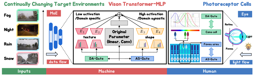
Figure 1: The problem and motivation. Our goal is to effectively adapt the source pre-trained model to continually changing target domains. We propose a Mixture-of-Experts (MoE) based to encode the different features of texture and shape with different experts. Our design is inspired by the photoreceptor cells in the human visual system, where the three types of cone cells are sensitive to different wavelengths of light and the Fovea.

The renowned Trichromatic Theory[26] demonstrates that the Retina in the human eye consists of different types of cone cells[27], each sensitive to specific light wavelengths. This photoreceptor cells are densely packed in the Fovea[28], an area highly sensitive to detail and essential for high-resolution vision tasks to enable self-attention, while other cone cells work with additional rod cells to manage perception in less focused areas of the visual field as well as the dimly lit environment, as shown in the blue part of the Fig. 1. Similarly, deep neural networks (DNN) also exhibit parallel characteristics which have been proven by previous works[29, 30, 31, 32] that strongly activated neuron encodes shape and structure, which are domain agnostic, while weak activation corresponds to domain-specific texture and style. Therefore, we can delineate the conceptual associations between {low/high activation}-{domain specific/agnostic}-{texture/shape}. Drawing inspiration from the human visual system and the prior research, we propose an intriguing hypothesis: $\spadesuit$ Can we explicitly decompose neurons by activation degree to encode shapes and textures separately for better model perception to differentiate the continuously changing environments?

To demystify the role of activation sparsity in CTTA, we manually decompose strongly and weakly activated neurons in a pretrained and visualize their responses to inputs from varying domains in Fig. 2. We observe a clear distinction in the neuron attention, where strongly activated neurons focus on domain-agnostic foreground features relating to the main object; while weakly activated neurons attend to domain-specific background features of styles and noises. This motivates our study on the explicit decomposition of neural activation with a sparse Mixture-of-Experts (MoE)[33, 34, 35, 36, 37] architecture to mimic the partitioned processing of visual signals by the Fovea and peripheral regions in the Retina[38]. We propose the Mixture-of-Activation-Sparsity-Experts (MoASE), an adapter integrated into pre-trained models, featuring a non-differentiable Spatial Differentiate Dropout (SDD) mechanism. This setup enhances the extraction of domain-agnostic object shapes and structures and identifies domain-specific textures from a spatial-wise perspective, such as weather-related noise from fog and snow[11] through specialized expert modules, whose functionality is highlighted in the red section of Fig. 1.

Moreover, we developed a multi-gate module to enhance dynamic perception in the fluctuating CTTA scenario[15, 16, 20, 21, 22, 23], comprising the Domain Aware Gate (DAG) to inform the experts with domain-specific information and the Activation Sparsity Gate (ASG) to adjust the threshold of activation selection for each expert. Moreover, to mitigate error accumulation caused by the random initialization of the injected MoASE, we have devised a Homeostatic-Proximal (HP) loss to regularize and balance the updates of domain-specific and domain-agnostic parameters.

Extensive experiments demonstrate the superiority of our proposed Mixture-of-Activation-Sparsity-Experts (MoASE) across three image classification benchmarks[39, 40] and one segmentation benchmark[41, 42] on CTTA scenarios with improvements exceeding 15.3% in classification accuracy and 5.5% in segmentation mIoU. The major contribution of our paper can be summarized as follows:

• We draw inspiration from the human visual system to develop a Mixture-of-Sparsity-Activation-Experts (MoASE) model, which addresses the issues of error accumulation and catastrophic forgetting to face the continuously changing distribution.

• We decompose the neuron-encoded activation into domain-specific and domain-agnostic features, using distinct expert models to encode texture and shape independently with Spatial Differentiate Dropout (SDD).

• We developed a multi-gate module featuring the Domain Aware Gate (DAG) and Activation Sparsity Gate (ASG), utilizing domain information to dynamically generate adaptive routing strategies and activation thresholds for experts.

• We propose a novel Homeostatic-Proximal (HP) loss to mitigate the accumulation error and enhance performance within the teacher-student framework. Extensive experiments demonstrate the efficacy of our MoASE across diverse CTTA scenarios.

2 Related works

Continual Test-Time Adaptation (CTTA) addresses the challenge of adapting to a non-static target domain, which complicates traditional TTA methods. The pioneering work by Wang et al. [15] combined bi-average pseudo labels with stochastic weight resets to tackle this issue. To mitigate error accumulation, Ecotta [16] employs a meta-network for output regularization. While these approaches focus on model-level solutions, other studies [43, 21, 44, 20] explore the use of visual domain prompts or minimal parameter adjustments for continual learning. Liu [23] introduced reconstruction techniques for continual adaptation, and BECotta [45] implemented a Mixture of Experts strategy in CTTA, promoting effective domain-specific knowledge retention. Unlike previous implicit methods, our MoASE adopts an explicit approach to this challenge.

Activation Sparsity refers to the presence of numerous weakly-contributing elements in activation outputs[46, 47, 48, 49]. SparseViT[50] revisits this concept for modern window-based vision transformers, aiming to increase speed and reduce computation. Grimaldi[51] introduces semi-structured activation sparsity that can be leveraged with minor runtime adjustments to significantly enhance speed on embedded devices. Meanwhile, Mirzadeh[52] explores the reuse of activated neurons in LLMs, proposing strategies to reduce computation. However, all the previous works aim to improve model efficiency until [30, 29] reveal the contribution of shape bias for model performance.

Mixture-of-Experts (MoE) is initially introduced by Jacobs and Jordan [33, 53], uses independent modules to boost expressiveness and cut computational costs. Eigen and Ma [54, 55] evolved it into the MoE layer. In natural language processing, GShard [56] and Switch Transformer [57] incorporated MoE with top-1/2 routing to enhance capacity. Fixed routing [58, 59] and ST-MoE [60] aimed to stabilize training. Recent developments [61, 36] introduced efficient adaptors within MoE and [62] combined MoE with implicit neural network for image compression. In computer vision, M³ViT by Liang et al. [63] selectively engages experts, while Zhang et al. [11] merged feature modulation with MoE for better image restoration. Our MoASE leverages a multi-expert setup to manage diverse neuronal activation.

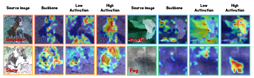
Figure 2: The visualization analysis of the Class Activation Map (CAM). We adopt CAM to compare the attention of the low-activation MoASE, high-activation MoASE, and the original model during the continual adaptation process.

3 Motivation

Drawing inspiration from the complexities of the human visual system [26, 27, 28] and reinforced by seminal findings in recent research [29, 30, 31, 32], we come up with the hypothesis of leveraging activation sparsity via the innovative integration of a parallel MoE for CTTA. This MoE employs a network of architecture-consistent experts, combined with the Spatial Differentiate Dropout technique, to effectively decompose activation neurons. Such a configuration not only enhances the model’s capability to perceive domain-agnostic object structures but also sharpens its accuracy in identifying domain-specific knowledge within dynamically changing environments.

To provide empirical support for our hypothesis, we extended our analysis to include a qualitative evaluation using Class Activation Mapping (CAM)[64] within the ImageNet-to-ImageNet-C CTTA scenario. As depicted in Fig. 2, our study explores feature representations in various target domains, each characterized by different activation intensities, including Gaussian and Elastic noise, as well as Snow and Fog weather conditions. Specifically, we selectively retained only the high or low activation values within the ViT-base model under the CTTA scenario[15]. Our findings reveal that models maintaining only weakly activated neurons primarily accentuate fluctuations in background noise while overlooking the foreground object. This implies that weakly activated neurons are adept at capturing domain-relevant information. Conversely, models with strongly activated neurons exhibit a contrasting pattern, focusing more intensively on object shapes and structures. This observation supports the notion that strongly activated neurons are sensitive to domain-agnostic object structures, thus validating previous visual science principles and our hypothesis.

4 Methods

4.1 Preliminary

Continual Test-Time Adaptation. We pre-train the model $\theta(y_{s}|x_{s})$ on source domain $D_{S}={(\mathcal{Y}_{S},\mathcal{X}_{S})}$ and adapt it to multiple target domains $D_{T_{i}}={\{\mathcal{X}_{\mathcal{T}_{i}}\}}_{i=1}^{n}$, where $n$ indicates the number of target datasets. Utilizing the robustness of mean teacher predictions [65, 66], we implement a teacher-student framework ($\theta^{\mathcal{T}}$ and $\theta^{\mathcal{S}}$) to maintain stability during adaptation[15, 22]. This adaptation process, which is unsupervised and single-pass for target domain data $x\in\mathcal{X}_{T}$, does not require access to source domain data. We aim to adapt the pre-trained model to continuously evolving target domains while maintaining recognition capabilities on familiar distributions. The framework and methodology are outlined in Fig. 3.

Mixture-of-Experts. The MoE model is fundamentally composed of $E$ expert functions $e_{i}:\mathcal{X}_{\mathcal{T}}\rightarrow\mathbb{R}^{p}$ for $i\in E$, alongside a trainable gating mechanism $g:\mathcal{X}_{\mathcal{T}}\rightarrow\mathbb{R}^{q}$ which allocates inputs to experts by outputting a probability vector. For an input sample $x$, the MoE’s output is the aggregate of expert contributions, each weighted by the router’s assigned probabilities, which can be mathematically represented with soft routing as:

$$y=\sum_{i=1}^{E}e_{i}(x)g_{i}(x),\ \ g(x)=\sigma(\boldsymbol{A}x+\boldsymbol{b})\quad s.t.\ \ g(x)\geq 0\ \ \text{and}\ \ \sum_{i=1}^{E}g_{i}(x)=1$$ (1)

where $\sigma(\cdot)$ signifies the softmax function, $\boldsymbol{A}\in\mathbb{R}^{n\times d}$ represents a matrix of trainable weights, and $\boldsymbol{b}\in\mathbb{R}^{n}$ is the bias vector. This gate operates densely, allocating nonzero probabilities to all experts.

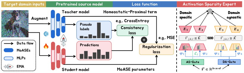
Figure 3: The overall framework of Mixture-of-Activation-Sparsity-Experts (MoASE). (Left) We integrate the MoASE into the linear layers of a pre-trained source model with a teacher-student framework, using consistency loss and a specially formulated Homeostatic-Proximal (HP) loss as the optimization target. (Right) Depending on the degree of distribution shift, we devised a multi-router structure that includes the Domain Aware Gate (DAG) and the Activation Sparsity Gate (ASG).

4.2 Mixture-of-Activation-Sparsity-Experts

Spatial Differentiate Dropout. We have adopted the sparse coding principle by incorporating a spatially oriented Top-K dropout operation in our framework. The MoASE architecture follows the same as previous MoE works[33, 53] with a gate $g(\cdot)$ and multiple experts $e(\cdot)$ with two linear layers. However, unlike traditional dropout layer between the linear layers that randomly discard $p(\%)$ of neuron activation on channel dimension, our MoASE incorporates the innovative Spatial Differentiate Dropout (SDD) that selectively retains the top/bottom $q(\%)$ significant responses from the spatial-wise token dimension following the non-linear activation function (e.g., ReLU) since the domain-related information was distributed across each token. Specifically, for an input feature $\mathcal{F}\in\mathbb{R}^{b\times n\times d}$, the SDD layer $\delta(\cdot)$ receive the non-linear-transformed activated feature and generate the $\hat{\mathcal{F}}\in\mathbb{R}^{b\times n\times d}$ with the sorting function $\delta=argsort(\mathcal{F},K,L)$:

$$\hat{\mathcal{F}}[j,k,l]:=\left\{\begin{aligned} \ \mathcal{F}[j,k,l],\quad&\text{if}\ \ \mathcal{F}[j,k,l]\ \geq\ argsort(\mathcal{F}[j,:,:])[K]\ \ \text{and}\ \ L=True\\ \ \mathcal{F}[j,k,l],\quad&\text{if}\ \ \mathcal{F}[j,k,l]\ \leq\ argsort(\mathcal{F}[j,:,:])[K]\ \ \text{and}\ \ L=False\\ \ 0,\quad&\text{otherwise}\end{aligned}\right.$$ (2)

where $K=\lfloor nd\times q\rfloor$ is the index, $L$ is the boolean variable in the $argsort(\cdot)$ function indicating whether to select the largest or smallest values. For the domain-agnostic experts $L$ is set to $True$, while for the domain-specific experts, $L$ is set to $False$. To ensure that different experts can precept different levels of activation, we set the threshold according to the number of experts as hyperparameters which are detailed in Appendix B.

Domain Aware Gate and Activation Sparsity Gate. To enhance dynamic perception in the fluctuating CTTA scenario [15, 16, 20, 21, 22, 23], we propose a multi-gate module consisting of the Domain Aware Gate (DAG) and the Activation Sparsity Gate (ASG). These gates provide domain-specific information and differentiate domain-agnostic objects for each expert. Both gates employ the architecture of $g(\cdot)$ described in Eq. 1, but serve distinct proposes. Specifically, the DAG determines the routing of input tokens across the experts. To better help the router adapt to diverse domains in the CTTA scenario, we specifically decompose low activations from the input feature $\mathcal{F}\in\mathbb{R}^{b\times n\times d}$ using the SDD layer with $q\%=\frac{1}{2}$,to let the router weight $G$ focuses more on domain-specific information. Simultaneously, the ASG uses the full input to generate a dynamic threshold $T\in\mathbb{R}^{1\times E}$ for SDD in each expert to facilitate adaptive activation decomposition in response to ongoing changes. The mathematics formulation can be described as:

$$G=DAG(\delta(\mathcal{F},\lfloor\frac{nd}{2}\rfloor,False)),\quad\quad T=ASG(\mathcal{F})$$ (3)

where $G\in\mathbb{R}^{b\times n\times E}$ is the expert weight. The thresholds generated by ASG are combined with predefined thresholds in Eq. 2 to compute the final $\hat{K}_{i}=\lfloor nd\times(q+\eta\cdot T_{i})\rfloor$ for each expert, where $\eta$ is a temperature scale that ensures $\hat{K}$ does not exceed the upper limit. This integration supports a responsive and balanced adaptation to the evolving scenario demands.

4.3 Optimization objective

Homeostatic-Proximal loss. Building on prior CTTA research  [15], we employ the teacher model $\theta^{\mathcal{T}}$ to generate pseudo labels $y_{pd}$ to minimize the task-specific training objective $\mathcal{L}_{TS}(\cdot)$, which are used to update MoASE. Despite the successful implementation of multiple experts to perceive various degrees of activation, we also strive to maintain statistical homeostasis amid continuous domain shifts by constraining student updates $\theta^{\mathcal{S}}$ to stay closely aligned with the initial (teacher) model $\theta^{\mathcal{T}}$, thus eliminating the need for manual intervention. In particular, instead of just minimizing the $\mathcal{L}_{TS}(\cdot)$, we further introduce the Homeostatic-Proximal term to the original loss[15] to approximately minimize the following optimization objective $\mathcal{L}_{Overall}$:

$$\mathcal{L}_{Overall}=\mathcal{L}_{TS}(\theta^{\mathcal{S}})+\frac{\mu}{2}\sum_{e=1}^{E}||\theta_{e}^{\mathcal{S}}-\theta_{e}^{\mathcal{T}}||^{2}.$$ (4)

where $\mu$ is a hyperparameter, $\theta_{e}^{\mathcal{S}}$ and $\theta_{e}^{\mathcal{T}}$ represent the parameters of each expert in the MoASE teacher-student framework, respectively.

Exponential Moving Average. Moreover, as for the update of the teacher model, we initialize both models with source pre-trained parameters and use the Exponential Moving Average (EMA) approach to update the teacher model $\theta^{\mathcal{T}}$ following established practices [43]:

$$\theta^{\mathcal{T}}_{t}=\alpha\times\theta^{\mathcal{T}}_{t-1}+(1-\alpha)\times\theta^{\mathcal{S}}_{t}$$ (5)

In this setup, $t$ indicates the time step, and we set the update weight $\alpha=0.999$ [67].

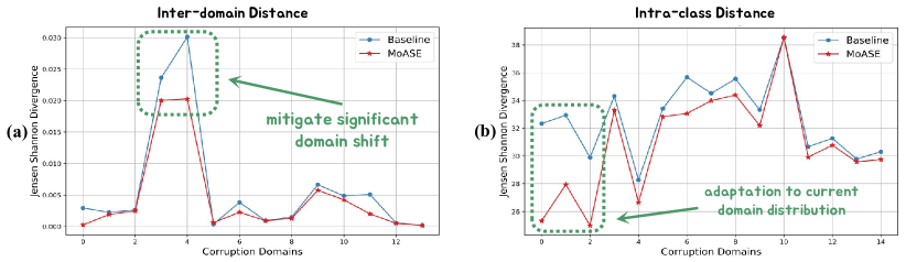
Figure 4: Inter-domain and intra-class distance. The X-axis displays the 15 corruption domains in CIFAR10-C, listed in sequential order. (a) MoASE more effectively reduces inter-domain divergence than the source model across all 14 domain shifts. (b) MoASE significantly improves intra-class feature aggregation, producing results that closely align with those of our proposed method.

5 Justification

To substantiate our hypothesis, we measure the domain representation of MoASE by calculating the distribution distance using Ben-David’s domain distance definition [68, 69] and the $\mathcal{H}$-divergence metric, building on previous domain transfer studies [70]. The $\mathcal{H}$-divergence between source domain $D_{S}$ and target domain $D_{T_{i}}$ is given as follows and error bound analysis can be found in Appendix A:

$$d_{\mathcal{H}}(D_{S},D_{T_{i}})=2\mathop{\mathrm{sup}}_{\mathcal{D}\sim\mathcal{H}}|\mathop{\mathrm{Pr}}_{x\sim D_{S}}[\mathcal{D}(x)=1]-\mathop{\mathrm{Pr}}_{x\sim D_{T_{i}}}[\mathcal{D}(x)=1]|$$ (6)

where $\mathcal{H}$ is the hypothesis space and $\mathcal{D}$ the discriminator. Consistent with the methodologies presented in [71, 72], we employ the $Jensen$-$Shannon\ (JS)\ divergence$ between two adjacent domains as an approximation of $\mathcal{H}$-divergence, owing to its demonstrated efficacy in differentiating between domains. A relatively small inter-domain divergence suggests that the feature representation is robust and exhibits reduced susceptibility to cross-domain shifts, as elaborated in [70]:

$$JS(P_{D_{S}}||P_{D_{T_{i}}})=\frac{1}{2}KL(P_{D_{S}}||\frac{P_{D_{S}}+P_{D_{T_{i}}}}{2})+\frac{1}{2}KL(P_{D_{T_{i}}}||\frac{P_{D_{S}}+P_{D_{T_{i}}}}{2}),$$ (7)

where $P$ denotes probability distribution of model output features and $KL(\cdot||\cdot)$ denotes the $Kullback-Leibler\ (KL)\ divergence$. As shown in Fig. 4(a), the MoASE shows significantly lower inter-domain divergence, indicating robust feature representation across domains. Moreover, we evaluate domain representation based on intra-class divergence, inspired by $k$-means clustering [73]. The mathematical representation can be formulated as:

$$IC=\frac{1}{|C|}\sum_{f_{i}\sim C}||f_{i}-\frac{1}{|C|}\sum_{f_{i}\sim C}f_{i}||_{2}^{2}$$ (8)

where $f_{i}$ is the encoder output feature from each domain. Smaller intra-class divergence indicates a superior understanding of the domain, as depicted for the in Fig. 4(b). The substantial and consistent margin between MoASE and the baseline model, as shown in Fig. 4, demonstrates the effectiveness of our proposed method in mitigating domain shifts.

6 Experiments

CTTA Task setting. Following [15], in classification CTTA tasks, we adapt the pre-trained source model sequentially across fifteen target domains on CIFAR10-C, CIFAR100C, and ImageNet-C exhibiting the highest level of corruption severity (level 5). In the context of segmentation CTTA, as per [21, 20], we employ an off-the-shelf model pre-trained on the Cityscapes dataset. For the continual adaptation to target domains, we utilize the ACDC dataset, which comprises images captured under four distinct adverse weather conditions: Fog→Night→Rain→Snow.

Implementation Details. For the backbone architectures in classification CTTA, we employ ViT-base [74], where we standardize input image sizes to 384$\times$384 for CIFAR and 224$\times$224 pixels for ImageNet. In segmentation CTTA, the Segformer-B5 model [14], pre-trained, serves as our source model, with input dimensions reduced from 1920x1080 to 960x540 for processing in target domains. $\eta$ is set to 0.1. Optimization utilizes the Adam algorithm [75] with $(\beta_{1},\beta_{2})=(0.9,0.99)$. Specific learning rates are assigned to each task: 1e-4 for classification, and 2e-4 for segmentation.

Table 1: Classification error rate(%) for ImageNet-to-ImageNet-C online CTTA task. Gain(%) represents the percentage of improvement in model accuracy compared with the source method.

Method Venue Gaussian shot impulse defocus glass motion zoom snow frost fog brightness contrast elastic_trans pixelate jpeg Mean$\downarrow$ Gain$\uparrow$ CIFAR10  $\Rightarrow$  CIFAR10-C Source[74] ICLR2021 60.1 53.2 38.3 19.9 35.5 22.6 18.6 12.1 12.7 22.8 5.3 49.7 23.6 24.7 23.1 28.2 0.0 TENT[76] CVPR2021 57.7 56.3 29.4 16.2 35.3 16.2 12.4 11.0 11.6 14.9 4.7 22.5 15.9 29.1 19.5 23.5 +4.7 CoTTA[15] CVPR2022 58.7 51.3 33.0 20.1 34.8 20 15.2 11.1 11.3 18.5 4.0 34.7 18.8 19.0 17.9 24.6 +3.6 VDP[43] AAAI2023 57.5 49.5 31.7 21.3 35.1 19.6 15.1 10.8 10.3 18.1 4.0 27.5 18.4 22.5 19.9 24.1 +4.1 ViDA[20] ICLR2024 52.9 47.9 19.4 11.4 31.3 13.3 7.6 7.6 9.9 12.5 3.8 26.3 14.4 33.9 18.2 20.7 +7.5 Ours Proposed 43.7 31.3 25.1 16.5 28.1 13.8 9.7 8.3 7.1 10.1 3.0 12.9 12.0 16.3 13.5 16.8 +11.4 CIFAR100  $\Rightarrow$  CIFAR100-C Source[74] ICLR2021 55.0 51.5 26.9 24.0 60.5 29.0 21.4 21.1 25.0 35.2 11.8 34.8 43.2 56.0 35.9 35.4 0.0 TENT[76] CVPR2021 53.0 47.0 24.6 22.3 58.5 26.5 19.0 21.0 23.0 30.1 11.8 25.2 39.0 47.1 33.3 32.1 +3.3 CoTTA[15] CVPR2022 55.0 51.3 25.8 24.1 59.2 28.9 21.4 21.0 24.7 34.9 11.7 31.7 40.4 55.7 35.6 34.8 +0.6 VDP[43] AAAI2023 54.8 51.2 25.6 24.2 59.1 28.8 21.2 20.5 23.3 33.8 7.5 11.7 32.0 51.7 35.2 32.0 +3.4 ViDA[20] ICLR2024 50.1 40.7 22.0 21.2 45.2 21.6 16.5 17.9 16.6 25.6 11.5 29.0 29.6 34.7 27.1 27.3 +8.1 Ours Proposed 42.6 34.2 20.5 23.1 38.7 22.2 17.3 18.8 18.0 24.1 12.7 24.4 28.2 32.7 29.0 25.8 +9.6 ImageNet  $\Rightarrow$  ImageNet-C Source[74] ICLR2021 53.0 51.8 52.1 68.5 78.8 58.5 63.3 49.9 54.2 57.7 26.4 91.4 57.5 38.0 36.2 55.8 0.0 TENT[76] CVPR2021 52.2 48.9 49.2 65.8 73 54.5 58.4 44.0 47.7 50.3 23.9 72.8 55.7 34.4 33.9 51.0 +4.8 CoTTA[15] CVPR2022 52.9 51.6 51.4 68.3 78.1 57.1 62.0 48.2 52.7 55.3 25.9 90.0 56.4 36.4 35.2 54.8 +1.0 VDP[43] AAAI2023 52.7 51.6 50.1 58.1 70.2 56.1 58.1 42.1 46.1 45.8 23.6 70.4 54.9 34.5 36.1 50.0 +5.8 ViDA[20] ICLR2024 47.7 42.5 42.9 52.2 56.9 45.5 48.9 38.9 42.7 40.7 24.3 52.8 49.1 33.5 33.1 43.4 +12.4 Ours Proposed 43.1 38.4 36.8 54.7 52.2 41.2 48.3 37.7 35.6 41.1 25.2 63.5 34.7 27.7 28.3 40.5 +15.3

6.1 Quantitative analysis

The effectiveness on classification CTTA validate the effectiveness of our method, we conduct experiments on CIFAR10-to-CIFAR10-C, CIFAR100-to-CIFAR100-C, and ImageNet-to-ImageNet-C, which consists of fifteen corruption types that occur sequentially during the test time, in Tab. 1. For MoASE, the average classification error is up to 55.8% when we directly test the source model on target domains with ImageNet-C. Our method can outperform all previous methods, achieving a 15.3% and 2.9% improvement over the source model and previous SOTA method, respectively. Moreover, our method showcases remarkable performance across the majority of corruption types, highlighting its effective mitigation of error accumulation and catastrophic forgetting.

The effectiveness on segmentation CTTA As presented in Tab. 2, we observed a gradual decrease in the mIoUs of TENT and DePT over time, indicating the occurrence of catastrophic forgetting. In contrast, our method has a continual improvement of average mIoU (61.8→62.3→62.3) when the same sequence of target domains is repeated. Significantly, the proposed method surpasses the previous SOTA CTTA method [15] by achieving a 4.0% increase in mIoU. This notable improvement showcases our method’s ability to adapt continuously to dynamic target domains in segmentation.

Adaptation across various model backbone. We evaluate the flexibility of our MoASE with Segformer-B0[14] and introduce the foundation model SAM[77] as the pre-trained model and adapt them to continual target domains in the Cityscapes-to-ACDC CTTA scenario. Our method significantly enhanced performance in dynamic target domains, as shown in Tab. 4, achieving improvements of 0.6% and 0.4% for Segformer-B0 and SAM-SETR, respectively. These findings confirm that the MoASE supports effective transfer learning across model sizes and is well-suited for a variety of real-world applications, including those in resource-limited environments like autonomous driving. Note that, we only use the pre-trained encoder of SAM[77] loaded into SETR model[78] and add a classification head, which is fine-tuned on the source domain.

Exploration on domain generalization. To evaluate the domain generalization (DG) capabilities of our method, we employed a leave-one-domain-out approach [79, 80], training on 10 of the 15 ImageNet-C domains and using the remaining 5 as unsupervised target domains. Our method adapts a pre-trained model to these 10 domains, then tests directly on the five unseen domains, as shown in Tab. 4. Impressively, it reduces average error in these domains by 12.4%, outperforming other approaches such as ViDA by over 4.8%. These results confirm our method’s effectiveness in enhancing DG capabilities. More experiment results are in Appendices C, D, E, F, G and H.

Table 2: Performance comparison for Cityscape-to-ACDC CTTA. We sequentially repeat the same sequence of target domains three times. C-MAE stands for Continual-MAE. Mean is the average score of mIoU.

Time $t$ Round 1 2 3 Mean$\uparrow$ Gain$\uparrow$ Method Venue Fog Night Rain Snow Mean$\uparrow$ Fog Night Rain Snow Mean$\uparrow$ Fog Night Rain Snow Mean$\uparrow$ Source[14] NIPS2021 69.1 40.3 59.7 57.8 56.7 69.1 40.3 59.7 57.8 56.7 69.1 40.3 59.7 57.8 56.7 56.7 0.0 CoTTA[15] CVPR2022 70.9 41.2 62.4 59.7 58.6 70.9 41.1 62.6 59.7 58.6 70.9 41.0 62.7 59.7 58.6 58.6 +1.9 VDP[43] AAAI2023 70.5 41.1 62.1 59.5 58.3 70.4 41.1 62.2 59.4 58.2 70.4 41.0 62.2 59.4 58.2 58.2 +1.5 DAT[44] ICRA2024 71.7 44.4 65.4 62.9 61.1 71.6 45.2 63.7 63.3 61.0 70.6 44.2 63.0 62.8 60.2 60.8 +4.1 SVDP[21] AAAI2024 72.1 44.0 65.2 63.0 61.1 72.2 44.5 65.9 63.5 61.5 72.1 44.2 65.6 63.6 61.4 61.1 +4.4 ViDA[20] ICLR2024 71.6 43.2 66.0 63.4 61.1 73.2 44.5 67.0 63.9 62.2 73.2 44.6 67.2 64.2 62.3 61.9 +5.2 C-MAE[23] CVPR2024 71.9 44.6 67.4 63.2 61.8 71.7 44.9 66.5 63.1 61.6 72.3 45.4 67.1 63.1 62.0 61.8 +5.1 Ours Proposed 72.4 44.5 66.4 63.8 61.8 73.0 45.1 67.5 63.5 62.3 73.5 44.5 67.4 63.5 62.3 62.2 +5.5

Table 3: Different size of model backbone and foundation model. mIoU score for Cityscape-to-ACDC. Mean(%) is the average results in the first round.

Backbone	Method	Fog	Night	Rain	Snow	Mean$\uparrow$
Segformer-B0[14]	ViDA[20]	57.9	27.8	53.1	51.6	47.6
	Ours	58.2	28.7	53.6	52.2	48.2
SAM[77]-SETR [78]	ViDA[20]	76.5	47.2	68.1	70.7	65.6
	Ours	76.8	47.6	68.7	71.0	66.0

Table 4: The domain generalization comparisons on ImageNet-C. Results are evaluated on ViT-base. Mean(%) represents the performance on unseen target domains.

Method	bri.	contrast	elastic	pixelate	jpeg	Mean$\downarrow$
Source[14]	26.4	91.4	57.5	38.0	36.2	49.9
CoTTA[15]	25.3	88.1	55.7	36.4	34.6	48.0
ViDA[20]	24.6	68.2	49.8	34.7	34.1	42.3
Ours	25.4	65.5	37.3	29.5	29.6	37.5

6.2 Ablation study

Different number of experts. In this study, we evaluate the impact of varying expert module counts in the MoASE on mIoU scores under adverse weather conditions within the Cityscape-to-ACDC CTTA scenario, as shown in Tab. 6. We tested configurations with 2 to 16 expert modules. The baseline, with no experts, achieved a mean mIoU of 58.6%. Our findings reveal that a setup with four experts delivered the highest scores in Fog and Snow, achieving an overall mean mIoU of 61.8%. These results demonstrate that the relationship between the number of experts and model performance in CTTA is not linear; rather, precise activation decomposition is essential for optimal performance.

Effectiveness of each proposed module. We conducted an ablation study in the Cityscape-to-ACDC CTTA scenario to evaluate the effects of our modules including Spatial Differentiate Dropout (SDD), Domain Agnostic Gate (DAG), Activation Sparsity Gate (ASG), and Homeostatic-Proximal (HP) loss. Tab. 6 shows $Ex_{0}$ as the baseline using the CoTTA [15] and $Ex_{1}$ adding a 4-expert MoE architecture to $Ex_{0}$. However, simply adding MoE did not enhance performance; it instead decreased by 0.7%. In contrast, implementing our SDD in $Ex_{2}$ improved segmentation results by 3.2%. Further introductions of our modules from $Ex_{3}$ to $Ex_{5}$ increased mIoU from 61.5% to 62.2%, confirming the effectiveness of our proposed methods.

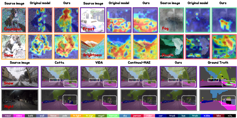
Figure 5: The qualitative analysis of the CAM and the segmentation qualitative comparison of our method with previous SOTA methods on the ACDC dataset.

Table 5: Different number of experts. mIoU score for Cityscape to ACDC with MoASE within the first round.

num. E.	Fog	Night	Rain	Snow	Mean$\uparrow$
$E=0$	70.9	41.2	62.4	59.7	58.6
$E=2$	71.6	44.0	66.5	63.7	61.5
$E=4$	72.4	44.5	66.4	63.8	61.8
$E=8$	71.4	44.0	65.0	61.7	60.5
$E=16$	71.5	44.1	65.9	63.3	61.2

Table 6: Ablation study on Cityscape to ACDC showing the effectiveness of each module.

	MoE	SDD	DAG	ASG	HP	Mean$\uparrow$
$Ex_{0}$	-	-	-	-	-	58.6
$Ex_{1}$	✓	-	-	-	-	57.9
$Ex_{2}$	✓	✓	-	-	-	61.1
$Ex_{3}$	✓	✓	✓	-	-	61.5
$Ex_{4}$	✓	✓	✓	✓	-	62.0
$Ex_{5}$	✓	✓	✓	✓	✓	62.2

6.3 Qualitative analysis

CAM visualization. We conducted a qualitative analysis of the CAM on ImageNet-C, as illustrated at the top of Fig. 5. MoASE effectively concentrates on regions relevant to the target categories, such as dogs and cars, during classification decisions. In contrast, the original model’s attention is dispersed due to continuous domain shifts. These findings underscore MoASE’s superiority.

Segmentation results. For further validation, we provide additional qualitative comparisons in the Cityscapes-to-ACDC CTTA scenario, shown at the bottom of Fig. 5. Our method outperforms CoTTA[15], ViDA[20], and Continual-MAE[23] in producing segmentation maps for snow and night domains, precisely differentiating sidewalks from roads and identifying small objects like people, vegetation, and fences (highlighted in the white box). These results highlight our method’s precise segmentation capabilities and robustness against dynamic domain shifts. Additionally, our segmentation maps align closely with the Ground Truth, leading to significant visual improvements.

7 Conclusion and limitations

Inspired by the human visual system where specialized cone cells perceive different light spectrum sections, this paper explores deep neural networks (DNNs) under the Continual Test-time Adaptation (CTTA) scenario. We introduce a novel architecture, the Mixture-of-Activation-Sparsity-Experts (MoASE). This design decouples neural activation into high-activation and low-activation components using Spatial Differentiate Dropout (SDD) and enhances domain-specific feature extraction while improving the perception of domain-agnostic objects through expert modules. Enhanced by a multi-gate module and Homeostatic-Proximal (HP) loss, MoASE surpasses state-of-the-art baselines in four benchmarks. However, the additional computational overhead introduced to the system can potentially be further minimized in future research. Exploring methods such as feature modulation or quantization could enhance model efficiency.

Appendix

The supplementary materials accompanying this paper provide a comprehensive quantitative and qualitative analysis of the proposed method. To begin with, we provide the error bound analysis in Appendix A. In Section Appendix B, we offer detailed insights into the experimental settings, including datasets and additional implementation specifics. Furthermore, we expand our investigation into the effects of varying middle-layer dimensions on CIFAR10-C performance in Section Appendix C. To evaluate the domain generalization capabilities of our method, we conducted experiments that directly tested its performance across a varying number of unseen domains, as detailed in Section Appendix D. Section Appendix E describes five rounds of semantic segmentation CTTA experiments, providing deeper insights into the method’s adaptability and effectiveness. Additionally, we include an experiment in Appendix F that elucidates our decision to apply Spatial Differentiate Dropout (SDD) on the spatial-wise token dimension rather than the channel dimension, highlighting the strategic rationale behind this choice. Finally, Section Appendix H presents further qualitative analysis, offering a visual and descriptive exploration of the method’s performance enhancements and capabilities.

Appendix A A bound relating the source and target error

We now turn our attention to establishing bounds on the target domain generalization performance of a discriminator trained within the source domain. Initially, we aim to quantify the target error about the source error[68, 69], the discrepancy between the labeling functions $f_{S}$ and $f_{T}$, and the divergence between the distributions $D_{S}$ and $D_{T}$. Given the practical assumption that the difference between labeling functions is minimal, our analysis primarily concentrates on quantifying distribution divergence. Particularly, we explore methods for estimating this divergence using finite samples of unlabeled data from $D_{S}$ and $D_{T}$. A pertinent measure for evaluating divergence between distributions is the variation divergence:

$$d(D,D^{\prime})=2\mathop{\mathrm{sup}}_{W\in\mathcal{W}}|\mathrm{Pr}_{D}[W]-\mathrm{Pr}_{D^{\prime}}[W]|$$ (9)

where $\mathcal{W}$ represents the set of measurable subsets with respect to distributions $D$ and $D^{\prime}$. We employ this measure to establish an initial bound on the target error of a discriminator.

Theorem 1

For a hypothesis h,

$$\epsilon_{T}(h)\leq\epsilon_{S}(h)+d(D,D^{\prime})+min\{E_{D}[|f_{S}(\textbf{x})-f_{T}(\textbf{x})|],E_{D^{\prime}}[|f_{S}(\textbf{x})-f_{T}(\textbf{x})|]\}$$ (10)

Proof 1

Given that $\epsilon_{T}(h)=\epsilon_{T}(h,f_{T})$ and $\epsilon_{S}(h)=\epsilon_{S}(h,f_{S})$, let $\phi_{S}$ and $\phi_{T}$ denote the density functions of distributions $D$ and $D^{\prime}$, respectively.

$$\epsilon_{T}(h) =\epsilon_{T}(h)+\epsilon_{S}(h)-\epsilon_{S}(h)+\epsilon_{S}(h,f_{T})-\epsilon_{S}(h,f_{T})$$ (11)

$$\leq\epsilon_{S}(h)+|\epsilon_{S}(h,f_{T})-\epsilon_{S}(h,f_{S})|+|\epsilon_{T}(h,f_{T})-\epsilon_{S}(h,f_{T})|$$ (12)

$$\leq\epsilon_{S}(h)+E_{D}[|f_{S}(\textbf{x})-f_{T}(\textbf{x})|]+|\epsilon_{T}(h,f_{T})-\epsilon_{S}(h,f_{T})|$$ (13)

$$\leq\epsilon_{S}(h)+E_{D}[|f_{S}(\textbf{x})-f_{T}(\textbf{x})|]+\int|\phi_{S}(\textbf{x})-\phi_{T}(\textbf{x})||h(\textbf{x})-f_{T}(\textbf{x})|d\textbf{x}$$ (14)

$$\leq\epsilon_{S}(h)+E_{D}[|f_{S}(\textbf{x})-f_{T}(\textbf{x})|]+d(D,D^{\prime})$$ (15)

In the first line, we can alternatively add and subtract $\epsilon_{T}(h,f_{S})$ instead of $\epsilon_{T}(h,f_{T})$. This adjustment leads to the same theoretical bound, albeit with the expectation calculated concerning distribution $D^{\prime}$ rather than $D$. Choosing the smaller of the two bounds provides a more favorable constraint.

However, approximating the error of the optimal hyperplane discriminator for arbitrary distributions is recognized as an NP-hard problem. In response, we approximate the optimal hyperplane discriminator by minimizing a convex upper bound on the error, a common approach in classification. It is crucial to recognize that this method does not yield a valid upper bound on the target error. Therefore, we utilize the $Jensen$-$Shannon\ (JS)\ divergence$ between two adjacent domains as an approximation of $\mathcal{H}$-divergence with respect to $d(D,D^{\prime})$.

Appendix B Detailed experiment settings

Following [15], in classification CTTA tasks, the model’s online prediction capabilities are evaluated immediately upon processing the input data. To mimic real-life scenarios of environmental change, we cyclically expose the model to these conditions in a repeated sequence (Fog→Night→Rain→Snow) across multiple cycles.

Dataset. We evaluate our method on three classification CTTA benchmarks: CIFAR10-to-CIFAR10C, CIFAR100-to-CIFAR100C [39], and ImageNet-to-ImageNet-C [40]. CIFAR10-C, CIFAR100-C, and ImageNet-C are specifically designed to test the robustness of machine learning models against common real-world image corruptions and perturbations, including noise, blur, and compression. For the segmentation CTTA context [21, 20], we conduct evaluations using the Cityscapes-to-ACDC benchmark. Cityscapes dataset [41] is used as the source domain, while the ACDC dataset [42] serves as the target domain, assessing adaptation effectiveness.

Implementation Details. In our CTTA experiments, we meticulously adhere to the implementation protocols established in previous research [15] to ensure both consistency and comparability across our studies. As part of our augmentation strategy, we employ a range of image resolution scaling factors [0.5, 0.75, 1.0, 1.25, 1.5, 1.75, 2.0] to generate inputs for the teacher model, as suggested by Wang et al. [15]. The batch size is set to 40 according to ViDA[20]. For the segmentation task, the learning rate decay is set at 0.5 for each 3200 iterations. The hyperparameter $\mu$ in Eq. 4 is set to 1, aligning with the findings from previous studies [81]. The threshold is manually set for SDD as $q\%=\{\frac{id_{h}}{E},...,\frac{1}{2},\frac{id_{l}}{E},...,\frac{1}{2}\}$, where $id_{h}$ and $id_{l}$ suggests the expert ID for domain-agnostic experts and domain-specific experts. In the initialization process of the MoASE, we adopt the methodology from Adaptformer [82]. The weights of the down-projection layers are initialized using Kaiming Normal initialization [83], which is well-suited for preserving the mean and variance of inputs through the layers during forward and backward passes. Conversely, the biases in the additional networks and the weights of the up-projection layers are set to zero. This combination of initialization is designed to optimize the performance and stability of the model during training, ensuring that each component contributes effectively to the overall learning process. The random seed is set to 1.

Table 7: Classification error rate(%) for CIFAR10-to-CIFAR10-C online CTTA task. Gain(%) represents the percentage of improvement in model accuracy compared with the source method with different hidden size $h$ in Activation Sparsity Experts.

Method Gaussian shot impulse defocus glass motion zoom snow frost fog brightness contrast elastic pixelate jpeg Mean$\downarrow$ $Ex_{1}$ Source 60.1 53.2 38.3 19.9 35.5 22.6 18.6 12.1 12.7 22.8 5.3 49.7 23.6 24.7 23.1 28.2 $Ex_{2}$ CoTTA 58.7 51.3 33.0 20.1 34.8 20 15.2 11.1 11.3 18.5 4.0 34.7 18.8 19.0 17.9 24.6 $Ex_{3}$ $h=24$ 65.4 56.3 32.8 16.2 31.4 13.5 9.4 8.8 8.3 10.6 3.0 16.1 12.1 15.5 13.3 20.8 $Ex_{4}$ $h=48$ 43.7 31.3 25.1 16.5 28.1 13.8 9.7 8.3 7.1 10.1 3.0 12.9 12.0 16.3 13.5 16.8 $Ex_{5}$ $h=96$ 63.4 52.4 36.4 18.7 31.9 15.4 11.2 9.7 8.5 12.0 3.3 15.5 12.8 17.1 14.2 21.5 $Ex_{6}$ $h=192$ 59.1 47.7 27.4 16.0 28.6 13.0 9.2 8.4 7.7 9.8 3.0 14.5 12.3 15.5 13.2 19.0

Appendix C How does the middle-layer dimension influence the performance?

According to the results presented in Tab. 7, the table provides a comparative analysis of the baseline method’s performance against three experimental configurations with hidden sizes of 24, 48, 96, and 192 on the CIFAR10-to-CIFAR10-C online CTTA task. An interesting observation from the table is that the correlation between model performance and the size of the hidden dimension does not follow a linear trend. Specifically, a hidden size of $h=48$ demonstrates optimal model performance with a mean error rate of 16.8%, whereas a smaller hidden size of $h=24$ results in a higher error rate of 20.8% where the larger hidden size of $h=96$ with an even higher error rate of 21.5%. Moreover, further increasing the hidden dimension to $h=192$ does not yield a significant improvement in performance, with the error rate marginally reduced to 19.0%, but it entails a substantial increase in the model size.

The nonlinear relationship between model architecture and task complexity is critical in resource-limited settings like mobile computing or autonomous driving, where efficient yet effective models are essential. Therefore, we selected a hidden size of $h=48$ for our experiments to best balance performance and computational efficiency.

Appendix D Domain generalization on a different number of unseen target domains

Table 8: The domain generalization experiments on ImageNet-C, where the source model was continually adapted on the first 5 domains and directly tested on 10 unseen domains. The evaluation of the results was conducted using ViT-base.

	Directly test on 10 unseen domains										Unseen
Method	motion	zoom	snow	frost	fog	brightness	contrast	elastic_trans	pixelate	jpeg	Mean$\downarrow$
Source[14]	58.5	63.3	49.9	54.2	57.7	26.4	91.4	57.5	38.0	36.2	53.3
TENT[76]	56.0	61.3	45.7	49.6	56.6	24.8	94.0	55.6	37.1	35.1	51.6
CoTTA[15]	57.3	62.1	49.1	52.0	57.1	26.4	91.9	57.1	37.6	35.3	52.6
ViDA[20]	46.4	52.7	39.8	43.7	42.2	23.5	71.5	49.6	33.9	33.3	43.7
Ours	43.9	53.7	38.0	37.6	46.0	24.0	66.0	42.8	28.9	29.6	41.0

In this study, we adhere to the leave-one-domain-out principle, similar to previous works [79, 80]. We select a subset of ImageNet-C domains as new source domains for model updating while designating the remaining domains as target domains where no adaptation occurs. This approach diverges from earlier domain generalization experiments; here, we implement an unsupervised continual test-time adaptation (CTTA) approach, updating the model solely on these unlabeled source domains. The initial model weights are derived exclusively from ImageNet pre-trained parameters.

We specify that 5 out of 15 domains from ImageNet-C are used as source domains, with the other 10 and 8 out of 15 domains serving as unseen target domains. The results, as detailed in Tab. 8, are noteworthy. Our method achieves a significant reduction of 12.3% in average error across these unseen domains. These encouraging results validate the domain generalization (DG) capabilities of our approach, demonstrating its effectiveness in extracting domain-shared knowledge. This success offers a novel perspective on enhancing DG performance within an unsupervised framework.

Table 9: 5 rounds segmentation CTTA on Cityscape-to-ACDC. We sequentially repeat the same sequence of target domains 5 times with different number of experts in our proposed MoASE. Mean is the average score of mIoU.

Round 1 2 3 4 5 Mean Method Fog Night Rain Snow Mean Fog Night Rain Snow Mean Fog Night Rain Snow Mean Fog Night Rain Snow Mean Fog Night Rain Snow Mean Source 69.1 40.3 59.7 57.8 56.7 69.1 40.3 59.7 57.8 56.7 69.1 40.3 59.7 57.8 56.7 56.7 40.3 59.7 57.8 56.7 56.7 40.3 59.7 57.8 56.7 56.7 CoTTA 70.9 41.2 62.4 59.7 58.6 70.9 41.1 62.6 59.7 58.6 70.9 41.0 62.7 59.7 58.6 70.9 41.0 62.7 59.7 58.6 70.9 41.0 62.8 59.7 58.6 58.6 CoTTA^∗ 71.4 45.1 66.8 63.0 61.8 71.9 43.3 65.9 61.8 60.7 70.1 39.5 63.0 60.6 58.3 68.1 39.8 62.0 60.0 57.4 68.0 38.3 62.0 59.8 57.0 59.0 ViDA 71.6 43.2 66.0 63.4 61.1 73.2 44.5 67.0 63.9 62.2 73.2 44.6 67.2 64.2 62.3 70.9 44.0 66.0 63.2 61.0 72.0 43.7 66.3 63.1 61.3 61.6 E=2 71.6 44.0 66.5 63.8 61.5 72.7 45.6 67.5 63.9 62.3 72.5 44.6 67.5 63.0 62.0 71.8 44.4 67.3 63.3 61.7 71.3 43.2 66.8 62.3 60.9 61.7 E=4 72.4 44.5 66.4 63.8 61.8 73.0 45.1 67.5 63.5 62.3 73.5 44.5 67.4 63.5 62.3 71.8 44.3 66.3 62.7 61.3 72.0 44.1 66.5 62.2 61.2 61.8 E=8 71.4 44.0 65.0 61.7 60.5 72.3 43.5 65.5 62.0 60.8 71.6 43.1 64.6 61.4 60.2 71.2 42.5 64.7 62.4 60.2 70.6 43.3 65.2 61.4 60.1 60.4 E=16 71.5 44.1 65.9 63.3 61.2 72.7 44.6 67.3 63.3 62.0 72.2 43.5 67.8 63.0 61.6 71.3 43.2 67.3 62.3 61.0 70.8 43.0 66.7 61.8 60.6 61.3

Appendix E Additional experiments with different number of experts

We present the segmentation CTTA experiment across 5 rounds in Tab. 9, showing consistent mean mIoU enhancement during the initial rounds (1-3) and stable performance thereafter. Our method achieved a 0.2% mIoU improvement over the previous SOTA after averaging results from all rounds. Additionally, Tab. 9 (CoTTA^∗) details our adjustment of CoTTA’s hyperparameters, specifically increasing the learning rate to 2e-4. This change initially improves performance but leads to a decline in segmentation accuracy and catastrophic forgetting in later rounds.

Furthermore, we present the comprehensive results in Tab. 6 with different numbers of experts, which are detailed in the last four lines of Tab. 9. These results further underscore the robustness and flexibility of our proposed Mixture of Activation Sparsity Experts (MoASE), demonstrating its capability to achieve satisfactory outcomes across various experimental settings. Moreover, we observed a similar trend between the number of experts and the dimension of the hidden layer, suggesting that the appropriate activation decomposition is more crucial than the model size.

Table 10: Classification error rate(%) for ImageNet-to-ImageNet-C online CTTA task. Gain(%) represents the percentage of improvement in model accuracy compared with the source method.

Method Venue Gaussian shot impulse defocus glass motion zoom snow frost fog brightness contrast elastic_trans pixelate jpeg Mean$\downarrow$ Gain$\uparrow$ CIFAR10  $\Rightarrow$  CIFAR10-C Source[74] ICLR2021 60.1 53.2 38.3 19.9 35.5 22.6 18.6 12.1 12.7 22.8 5.3 49.7 23.6 24.7 23.1 28.2 0.0 CoTTA[15] CVPR2022 58.7 51.3 33.0 20.1 34.8 20 15.2 11.1 11.3 18.5 4.0 34.7 18.8 19.0 17.9 24.6 +3.6 Ours-Channel Proposed 59.2 48.0 28.1 15.8 29.5 13.5 9.3 8.4 7.7 10.2 3.3 13.6 12.1 15.6 13.3 19.2 +9.0 Ours-Token Proposed 52.4 40.1 25.6 16.2 28.5 13.7 9.5 8.1 7.3 10.2 3.1 14.0 12.0 15.6 13.6 18.0 +10.2

Appendix F Why conduct the SDD on spatial-wise token dimension instead of channel dimension?

In our experiments, we implemented Spatial Differentiate Dropout (SDD) on both the spatial-wise token dimension $n$ and the channel dimension $d$ of the input feature $\mathcal{F}\in\mathbb{R}^{b\times n\times d}$, as shown in Tab. 10. We observed that in most target domains, channel-wise MoASE maintained satisfactory performance levels that were comparable to those of spatial-wise MoASE, with an average error rate of 19.2% and a +9.0% improvement over the baseline from the source domain. However, in the first two target domains, implementing SDD specifically on the spatial-wise token dimension significantly enhanced model performance, reducing the error rate to an average of over 10%. We attribute this improvement to the distribution of domain-related information—such as styles and noises—across the entire images on each token. Consequently, decomposing the activation at the token dimension appears more effective for differentiating between domain-specific and domain-agnostic features, thereby tailoring the model more adeptly to the nuances of each domain.

Table 11: Analysis of computational costs for our proposed MoASE and previous SOTA baselines including a detailed comparison in terms of the number of parameters, FLOPs, and memory usage.

Round Parameters (M) FLOPs (GMac) GPU Memory (M) Method Venue Number Overhead (%) Number Overhead (%) Number Overhead (%) CoTTA[15] CVPR2022 173.14 - 650.72 - 20842 - ViDA[20] ICLR2024 177.95 2.8 668.25 2.7 22330 6.7 Ours Proposed 180.44 4.2 677.31 4.0 24530 17.6

Appendix G Computation analysis.

A primary concern in the Continual Test-Time Adaptation (CTTA) task is the requisite for computational efficiency, particularly in mobile computing applications such as autonomous driving vehicles, which are often constrained by limited computational resources. To address this issue, we present a detailed analysis of the computational costs of our proposed MoASE framework, including FLOPs, memory consumption, and model parameters with one Tesla A100, as shown in Tab. 11. It is observed that while MoASE incurs a slightly higher computational cost, the increase is modest with only 4.2% in a number of parameters, and 4.0% in FLOP—amounting to only a small percentage of the original model’s resources. This is juxtaposed against a substantial accuracy improvement of 15.3%, demonstrating the effectiveness of our approach in resource-constrained environments.

Appendix H More qualitative results.

To further validate the effectiveness of our proposed method, we have expanded our evaluation by providing additional qualitative Class Activation Map (CAM) visualizations across nine distinct target domains. These visualizations are coupled with comparative analyses in the challenging Cityscapes-to-ACDC Cross-Domain Task-Aware Adaptation (CTTA) scenario. The segmentation outputs, meticulously derived through the CTTA process, are vividly illustrated at the top and bottom of Fig. 6, respectively. These illustrations not only showcase the segmentation prowess of our method but also serve as a testament to the nuanced understanding of contextual discrepancies across different domains under th3cCTTA scenario.

The CAM visualizations, in particular, are pivotal in demonstrating the effectiveness of our MoASE method’s activation decomposition strategy. By focusing on specific areas of interest within the images, these maps reveal how our method enhances domain-specific feature extraction, thereby facilitating more precise and contextually relevant insights into the underlying segmentation process. The top part of Fig. 6 displays these class attention maps, highlighting areas where our method has successfully concentrated its attention, correlating strongly with regions of significant semantic importance within each target domain.

At the bottom of Fig. 6, our method’s segmentation maps are displayed, offering a direct comparison with those generated by competing methodologies such as CoTTA, ViDA, and Continual-MAE across two additional target domains. Our method excels particularly in distinguishing subtle yet critical features such as the sidewalk from the road. This capability is emphasized by a white box in the visualizations, which draws attention to the precise delineation achieved by our segmentation approach. This distinction is crucial as it not only underscores our method’s ability to produce more accurate segmentation outcomes but also highlights its robustness in effectively mitigating the impact of dynamic domain shifts.

Furthermore, in other categories beyond the highlighted examples, our method’s segmentation outputs exhibit a high degree of resemblance to the ground truth. This close alignment leads to notable visual enhancements and provides a strong indication of the method’s generalizability and effectiveness in handling diverse urban landscapes. The visual fidelity of these segmentation maps, coupled with the insightful CAM visualizations, collectively demonstrate the comprehensive capabilities of our proposed approach in adapting to and excelling within varied and dynamically changing environments.

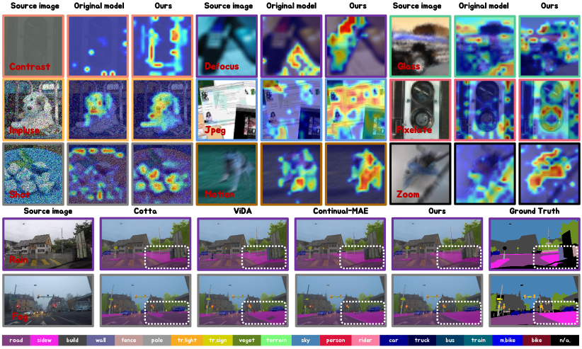
Figure 6: The qualitative analysis of the CAM and the segmentation qualitative comparison of our method with previous SOTA methods on the ACDC dataset.

References

- [1] Ekim Yurtsever, Jacob Lambert, Alexander Carballo, and Kazuya Takeda. A survey of autonomous driving: Common practices and emerging technologies. IEEE access, 8:58443–58469, 2020.
- [2] Jiaming Liu, Rongyu Zhang, Xiaowei Chi, Xiaoqi Li, Ming Lu, Yandong Guo, and Shanghang Zhang. Multi-latent space alignments for unsupervised domain adaptation in multi-view 3d object detection. arXiv preprint arXiv:2211.17126, 2022.
- [3] Xiaowei Chi, Jiaming Liu, Ming Lu, Rongyu Zhang, Zhaoqing Wang, Yandong Guo, and Shanghang Zhang. Bev-san: Accurate bev 3d object detection via slice attention networks. In Proceedings of the IEEE/CVF Conference on Computer Vision and Pattern Recognition, pages 17461–17470, 2023.
- [4] Siyu Teng, Xuemin Hu, Peng Deng, Bai Li, Yuchen Li, Yunfeng Ai, Dongsheng Yang, Lingxi Li, Zhe Xuanyuan, Fenghua Zhu, et al. Motion planning for autonomous driving: The state of the art and future perspectives. IEEE Transactions on Intelligent Vehicles, 2023.
- [5] Chenyu Yang, Yuntao Chen, Hao Tian, Chenxin Tao, Xizhou Zhu, Zhaoxiang Zhang, Gao Huang, Hongyang Li, Yu Qiao, Lewei Lu, et al. Bevformer v2: Adapting modern image backbones to bird’s-eye-view recognition via perspective supervision. In Proceedings of the IEEE/CVF Conference on Computer Vision and Pattern Recognition, pages 17830–17839, 2023.
- [6] Peter J Chen and David R Liu. Prime editing for precise and highly versatile genome manipulation. Nature Reviews Genetics, 24(3):161–177, 2023.
- [7] Xiaoqi Li, Mingxu Zhang, Yiran Geng, Haoran Geng, Yuxing Long, Yan Shen, Renrui Zhang, Jiaming Liu, and Hao Dong. Manipllm: Embodied multimodal large language model for object-centric robotic manipulation. arXiv preprint arXiv:2312.16217, 2023.
- [8] Xiaoqi Li, Yanzi Wang, Yan Shen, Ponomarenko Iaroslav, Haoran Lu, Qianxu Wang, Boshi An, Jiaming Liu, and Hao Dong. Imagemanip: Image-based robotic manipulation with affordance-guided next view selection. arXiv preprint arXiv:2310.09069, 2023.
- [9] Yihan Hu, Jiazhi Yang, Li Chen, Keyu Li, Chonghao Sima, Xizhou Zhu, Siqi Chai, Senyao Du, Tianwei Lin, Wenhai Wang, et al. Planning-oriented autonomous driving. In Proceedings of the IEEE/CVF Conference on Computer Vision and Pattern Recognition, pages 17853–17862, 2023.
- [10] William Gao, Noam Aigerman, Thibault Groueix, Vova Kim, and Rana Hanocka. Textdeformer: Geometry manipulation using text guidance. In ACM SIGGRAPH 2023 Conference Proceedings, pages 1–11, 2023.
- [11] Rongyu Zhang, Yulin Luo, Jiaming Liu, Huanrui Yang, Zhen Dong, Denis Gudovskiy, Tomoyuki Okuno, Yohei Nakata, Kurt Keutzer, Yuan Du, et al. Efficient deweahter mixture-of-experts with uncertainty-aware feature-wise linear modulation. In Proceedings of the AAAI Conference on Artificial Intelligence, volume 38, pages 16812–16820, 2024.
- [12] Lei Han, Tian Zheng, Lan Xu, and Lu Fang. Occuseg: Occupancy-aware 3d instance segmentation. In Proceedings of the IEEE/CVF conference on computer vision and pattern recognition, pages 2940–2949, 2020.
- [13] Xiaoyu Tian, Tao Jiang, Longfei Yun, Yucheng Mao, Huitong Yang, Yue Wang, Yilun Wang, and Hang Zhao. Occ3d: A large-scale 3d occupancy prediction benchmark for autonomous driving. Advances in Neural Information Processing Systems, 36, 2024.
- [14] Enze Xie, Wenhai Wang, Zhiding Yu, Anima Anandkumar, Jose M Alvarez, and Ping Luo. Segformer: Simple and efficient design for semantic segmentation with transformers. Advances in Neural Information Processing Systems, 34:12077–12090, 2021.
- [15] Qin Wang, Olga Fink, Luc Van Gool, and Dengxin Dai. Continual test-time domain adaptation. In Proceedings of the IEEE/CVF Conference on Computer Vision and Pattern Recognition, pages 7201–7211, 2022.
- [16] Junha Song, Jungsoo Lee, In So Kweon, and Sungha Choi. Ecotta: Memory-efficient continual test-time adaptation via self-distilled regularization. In Proceedings of the IEEE/CVF Conference on Computer Vision and Pattern Recognition, pages 11920–11929, 2023.
- [17] Dequan Wang, Evan Shelhamer, Shaoteng Liu, Bruno Olshausen, and Trevor Darrell. Tent: Fully test-time adaptation by entropy minimization. arXiv preprint arXiv:2006.10726, 2020.
- [18] Jian Liang, Ran He, and Tieniu Tan. A comprehensive survey on test-time adaptation under distribution shifts. arXiv preprint arXiv:2303.15361, 2023.
- [19] Dhanajit Brahma and Piyush Rai. A probabilistic framework for lifelong test-time adaptation. In Proceedings of the IEEE/CVF Conference on Computer Vision and Pattern Recognition, pages 3582–3591, 2023.
- [20] Jiaming Liu, Senqiao Yang, Peidong Jia, Ming Lu, Yandong Guo, Wei Xue, and Shanghang Zhang. Vida: Homeostatic visual domain adapter for continual test time adaptation. arXiv preprint arXiv:2306.04344, 2023.
- [21] Senqiao Yang, Jiarui Wu, Jiaming Liu, Xiaoqi Li, Qizhe Zhang, Mingjie Pan, and Shanghang Zhang. Exploring sparse visual prompt for cross-domain semantic segmentation. arXiv preprint arXiv:2303.09792, 2023.
- [22] Yulu Gan, Xianzheng Ma, Yihang Lou, Yan Bai, Renrui Zhang, Nian Shi, and Lin Luo. Decorate the newcomers: Visual domain prompt for continual test time adaptation. arXiv preprint arXiv:2212.04145, 2022.
- [23] Jiaming Liu, Ran Xu, Senqiao Yang, Renrui Zhang, Qizhe Zhang, Zehui Chen, Yandong Guo, and Shanghang Zhang. Adaptive distribution masked autoencoders for continual test-time adaptation. arXiv preprint arXiv:2312.12480, 2023.
- [24] Horace B Barlow. Retinal noise and absolute threshold. Josa, 46(8):634–639, 1956.
- [25] Darren Koenig and Heidi Hofer. The absolute threshold of cone vision. Journal of vision, 11(1):21–21, 2011.
- [26] Hermann Von Helmholtz. Handbuch der physiologischen Optik, volume 9. Voss, 1867.
- [27] Debarshi Mustafi, Andreas H Engel, and Krzysztof Palczewski. Structure of cone photoreceptors. Progress in retinal and eye research, 28(4):289–302, 2009.
- [28] Andreas Bringmann, Steffen Syrbe, Katja Görner, Johannes Kacza, Mike Francke, Peter Wiedemann, and Andreas Reichenbach. The primate fovea: structure, function and development. Progress in retinal and eye research, 66:49–84, 2018.
- [29] Tianqin Li, Ziqi Wen, Yangfan Li, and Tai Sing Lee. Emergence of shape bias in convolutional neural networks through activation sparsity. Advances in Neural Information Processing Systems, 36, 2024.
- [30] Rongyu Zhang, Yun Chen, Chenrui Wu, Fangxin Wang, and Bo Li. Multi-level personalized federated learning on heterogeneous and long-tailed data. arXiv preprint arXiv:2405.06413, 2024.
- [31] Yanchao Yang and Stefano Soatto. Fda: Fourier domain adaptation for semantic segmentation. In Proceedings of the IEEE/CVF Conference on Computer Vision and Pattern Recognition, pages 4085–4095, 2020.
- [32] Qinwei Xu, Ruipeng Zhang, Ya Zhang, Yanfeng Wang, and Qi Tian. A fourier-based framework for domain generalization. In Proceedings of the IEEE/CVF conference on computer vision and pattern recognition, pages 14383–14392, 2021.
- [33] Robert A Jacobs, Michael I Jordan, Steven J Nowlan, and Geoffrey E Hinton. Adaptive mixtures of local experts. Neural computation, 3(1):79–87, 1991.
- [34] Saeed Masoudnia and Reza Ebrahimpour. Mixture of experts: a literature survey. Artificial Intelligence Review, 42:275–293, 2014.
- [35] Carlos Riquelme, Joan Puigcerver, Basil Mustafa, Maxim Neumann, Rodolphe Jenatton, André Susano Pinto, Daniel Keysers, and Neil Houlsby. Scaling vision with sparse mixture of experts. Advances in Neural Information Processing Systems, 34:8583–8595, 2021.
- [36] Yijiang Liu, Rongyu Zhang, Huanrui Yang, Kurt Keutzer, Yuan Du, Li Du, and Shanghang Zhang. Intuition-aware mixture-of-rank-1-experts for parameter efficient finetuning. arXiv preprint arXiv:2404.08985, 2024.
- [37] Yanqi Zhou, Tao Lei, Hanxiao Liu, Nan Du, Yanping Huang, Vincent Zhao, Andrew M Dai, Quoc V Le, James Laudon, et al. Mixture-of-experts with expert choice routing. Advances in Neural Information Processing Systems, 35:7103–7114, 2022.
- [38] Greg D Field, Alapakkam P Sampath, and Fred Rieke. Retinal processing near absolute threshold: from behavior to mechanism. Annu. Rev. Physiol., 67:491–514, 2005.
- [39] Alex Krizhevsky, Geoffrey Hinton, et al. Learning multiple layers of features from tiny images. 2009.
- [40] Dan Hendrycks and Thomas Dietterich. Benchmarking neural network robustness to common corruptions and perturbations. arXiv preprint arXiv:1903.12261, 2019.
- [41] Marius Cordts, Mohamed Omran, Sebastian Ramos, Timo Rehfeld, Markus Enzweiler, Rodrigo Benenson, Uwe Franke, Stefan Roth, and Bernt Schiele. The cityscapes dataset for semantic urban scene understanding. In Proceedings of the IEEE conference on computer vision and pattern recognition, pages 3213–3223, 2016.
- [42] Christos Sakaridis, Dengxin Dai, and Luc Van Gool. Acdc: The adverse conditions dataset with correspondences for semantic driving scene understanding. In Proceedings of the IEEE/CVF International Conference on Computer Vision, pages 10765–10775, 2021.
- [43] Yulu Gan, Yan Bai, Yihang Lou, Xianzheng Ma, Renrui Zhang, Nian Shi, and Lin Luo. Decorate the newcomers: Visual domain prompt for continual test time adaptation. In Proceedings of the AAAI Conference on Artificial Intelligence, volume 37, pages 7595–7603, 2023.
- [44] Jiayi Ni, Senqiao Yang, Jiaming Liu, Xiaoqi Li, Wenyu Jiao, Ran Xu, Zehui Chen, Yi Liu, and Shanghang Zhang. Distribution-aware continual test time adaptation for semantic segmentation. arXiv preprint arXiv:2309.13604, 2023.
- [45] Daeun Lee, Jaehong Yoon, and Sung Ju Hwang. Becotta: Input-dependent online blending of experts for continual test-time adaptation. arXiv preprint arXiv:2402.08712, 2024.
- [46] Xuanyao Chen, Zhijian Liu, Haotian Tang, Li Yi, Hang Zhao, and Song Han. Sparsevit: Revisiting activation sparsity for efficient high-resolution vision transformer. In Proceedings of the IEEE/CVF Conference on Computer Vision and Pattern Recognition (CVPR), pages 2061–2070, June 2023.
- [47] Mark Kurtz, Justin Kopinsky, Rati Gelashvili, Alexander Matveev, John Carr, Michael Goin, William Leiserson, Sage Moore, Nir Shavit, and Dan Alistarh. Inducing and exploiting activation sparsity for fast inference on deep neural networks. In International Conference on Machine Learning, pages 5533–5543. PMLR, 2020.
- [48] Qing Yang, Jiachen Mao, Zuoguan Wang, and Hai Li. Dasnet: Dynamic activation sparsity for neural network efficiency improvement. In 2019 IEEE 31st International Conference on Tools with Artificial Intelligence (ICTAI), pages 1401–1405. IEEE, 2019.
- [49] Tzu-Hsien Yang, Hsiang-Yun Cheng, Chia-Lin Yang, I-Ching Tseng, Han-Wen Hu, Hung-Sheng Chang, and Hsiang-Pang Li. Sparse reram engine: Joint exploration of activation and weight sparsity in compressed neural networks. In Proceedings of the 46th International Symposium on Computer Architecture, pages 236–249, 2019.
- [50] Chenyang Song, Xu Han, Zhengyan Zhang, Shengding Hu, Xiyu Shi, Kuai Li, Chen Chen, Zhiyuan Liu, Guangli Li, Tao Yang, and Maosong Sun. Prosparse: Introducing and enhancing intrinsic activation sparsity within large language models, 2024.
- [51] Matteo Grimaldi, Darshan C. Ganji, Ivan Lazarevich, and Sudhakar Sah. Accelerating deep neural networks via semi-structured activation sparsity. In Proceedings of the IEEE/CVF International Conference on Computer Vision (ICCV) Workshops, pages 1179–1188, October 2023.
- [52] Iman Mirzadeh, Keivan Alizadeh, Sachin Mehta, Carlo C Del Mundo, Oncel Tuzel, Golnoosh Samei, Mohammad Rastegari, and Mehrdad Farajtabar. Relu strikes back: Exploiting activation sparsity in large language models, 2023.
- [53] Michael I Jordan and Robert A Jacobs. Hierarchical mixtures of experts and the EM algorithm. Neural computation, 6(2):181–214, 1994.
- [54] David Eigen, Marc’Aurelio Ranzato, and Ilya Sutskever. Learning factored representations in a deep mixture of experts. arXiv:1312.4314, 2013.
- [55] Jiaqi Ma, Zhe Zhao, Xinyang Yi, Jilin Chen, Lichan Hong, and Ed H Chi. Modeling task relationships in multi-task learning with multi-gate mixture-of-experts. In Proceedings of the ACM SIGKDD International Conference on Knowledge Discovery and Data Mining (KDD), 2018.
- [56] Dmitry Lepikhin, HyoukJoong Lee, Yuanzhong Xu, Dehao Chen, Orhan Firat, Yanping Huang, Maxim Krikun, Noam Shazeer, and Zhifeng Chen. Gshard: Scaling giant models with conditional computation and automatic sharding. In 9th International Conference on Learning Representations, ICLR 2021. OpenReview.net, 2021.
- [57] William Fedus, Barret Zoph, and Noam Shazeer. Switch transformers: Scaling to trillion parameter models with simple and efficient sparsity. CoRR, abs/2101.03961, 2021.
- [58] Stephen Roller, Sainbayar Sukhbaatar, Arthur Szlam, and Jason Weston. Hash layers for large sparse models. CoRR, abs/2106.04426, 2021.
- [59] Damai Dai, Li Dong, Shuming Ma, Bo Zheng, Zhifang Sui, Baobao Chang, and Furu Wei. Stablemoe: Stable routing strategy for mixture of experts. In Smaranda Muresan, Preslav Nakov, and Aline Villavicencio, editors, Proceedings of the 60th Annual Meeting of the Association for Computational Linguistics (Volume 1: Long Papers), ACL 2022, Dublin, Ireland, May 22-27, 2022, pages 7085–7095. Association for Computational Linguistics, 2022.
- [60] Barret Zoph. Designing effective sparse expert models. In IEEE International Parallel and Distributed Processing Symposium, IPDPS Workshops 2022, Lyon, France, May 30 - June 3, 2022, page 1044. IEEE, 2022.
- [61] Yun Zhu, Nevan Wichers, Chu-Cheng Lin, Xinyi Wang, Tianlong Chen, Lei Shu, Han Lu, Canoee Liu, Liangchen Luo, Jindong Chen, et al. Sira: Sparse mixture of low rank adaptation. arXiv preprint arXiv:2311.09179, 2023.
- [62] Jianchen Zhao, Cheng-Ching Tseng, Ming Lu, Ruichuan An, Xiaobao Wei, He Sun, and Shanghang Zhang. Moec: Mixture of experts implicit neural compression. arXiv preprint arXiv:2312.01361, 2023.
- [63] Hanxue Liang, Zhiwen Fan, Rishov Sarkar, Ziyu Jiang, Tianlong Chen, Kai Zou, Yu Cheng, Cong Hao, and Zhangyang Wang. M3 ViT: Mixture-of-experts vision transformer for efficient multi-task learning with model-accelerator co-design. In Advances in Neural Information Processing Systems (NIPS), 2022.
- [64] Bolei Zhou, Aditya Khosla, Agata Lapedriza, Aude Oliva, and Antonio Torralba. Learning deep features for discriminative localization. In Proceedings of the IEEE conference on computer vision and pattern recognition, pages 2921–2929, 2016.
- [65] Antti Tarvainen and Harri Valpola. Mean teachers are better role models: Weight-averaged consistency targets improve semi-supervised deep learning results. Advances in neural information processing systems, 30, 2017.
- [66] Mario Döbler, Robert A Marsden, and Bin Yang. Robust mean teacher for continual and gradual test-time adaptation. In Proceedings of the IEEE/CVF Conference on Computer Vision and Pattern Recognition, pages 7704–7714, 2023.
- [67] Antti Tarvainen and Harri Valpola. Mean teachers are better role models: Weight-averaged consistency targets improve semi-supervised deep learning results. Learning, 2017.
- [68] Shai Ben-David, John Blitzer, Koby Crammer, and Fernando Pereira. Analysis of representations for domain adaptation. Advances in neural information processing systems, 19, 2006.
- [69] Shai Ben-David, John Blitzer, Koby Crammer, Alex Kulesza, Fernando Pereira, and Jennifer Wortman Vaughan. A theory of learning from different domains. Machine learning, 79(1):151–175, 2010.
- [70] Yaroslav Ganin, Evgeniya Ustinova, Hana Ajakan, Pascal Germain, Hugo Larochelle, François Laviolette, Mario Marchand, and Victor Lempitsky. Domain-adversarial training of neural networks. The journal of machine learning research, 17(1):2096–2030, 2016.
- [71] Sebastian Ruder and Barbara Plank. Learning to select data for transfer learning with bayesian optimization. arXiv preprint arXiv:1707.05246, 2017.
- [72] Emily Allaway, Malavika Srikanth, and Kathleen McKeown. Adversarial learning for zero-shot stance detection on social media. arXiv preprint arXiv:2105.06603, 2021.
- [73] J MacQueen. Classification and analysis of multivariate observations. In 5th Berkeley Symp. Math. Statist. Probability, pages 281–297. University of California Los Angeles LA USA, 1967.
- [74] Alexey Dosovitskiy, Lucas Beyer, Alexander Kolesnikov, Dirk Weissenborn, Xiaohua Zhai, Thomas Unterthiner, Mostafa Dehghani, Matthias Minderer, Georg Heigold, Sylvain Gelly, et al. An image is worth 16x16 words: Transformers for image recognition at scale. arXiv preprint arXiv:2010.11929, 2020.
- [75] Diederik P Kingma and Jimmy Ba. Adam: A method for stochastic optimization. arXiv preprint arXiv:1412.6980, 2014.
- [76] Dequan Wang, Evan Shelhamer, Shaoteng Liu, Bruno A. Olshausen, and Trevor Darrell. Tent: Fully test-time adaptation by entropy minimization. In ICLR, 2021.
- [77] Alexander Kirillov, Eric Mintun, Nikhila Ravi, Hanzi Mao, Chloe Rolland, Laura Gustafson, Tete Xiao, Spencer Whitehead, Alexander C Berg, Wan-Yen Lo, et al. Segment anything. arXiv preprint arXiv:2304.02643, 2023.
- [78] Sixiao Zheng, Jiachen Lu, Hengshuang Zhao, Xiatian Zhu, Zekun Luo, Yabiao Wang, Yanwei Fu, Jianfeng Feng, Tao Xiang, Philip HS Torr, et al. Rethinking semantic segmentation from a sequence-to-sequence perspective with transformers. In Proceedings of the IEEE/CVF conference on computer vision and pattern recognition, pages 6881–6890, 2021.
- [79] Kaiyang Zhou, Ziwei Liu, Yu Qiao, Tao Xiang, and Chen Change Loy. Domain generalization in vision: A survey. arXiv preprint arXiv:2103.02503, 2021.
- [80] Da Li, Yongxin Yang, Yi-Zhe Song, and Timothy M Hospedales. Deeper, broader and artier domain generalization. In Proceedings of the IEEE international conference on computer vision, pages 5542–5550, 2017.
- [81] Tian Li, Anit Kumar Sahu, Manzil Zaheer, Maziar Sanjabi, Ameet Talwalkar, and Virginia Smith. Federated optimization in heterogeneous networks. Proceedings of Machine learning and systems, 2:429–450, 2020.
- [82] Shoufa Chen, Chongjian Ge, Zhan Tong, Jiangliu Wang, Yibing Song, Jue Wang, and Ping Luo. Adaptformer: Adapting vision transformers for scalable visual recognition. Advances in Neural Information Processing Systems, 35:16664–16678, 2022.
- [83] Kaiming He, Xiangyu Zhang, Shaoqing Ren, and Jian Sun. Delving deep into rectifiers: Surpassing human-level performance on imagenet classification. In Proceedings of the IEEE international conference on computer vision, pages 1026–1034, 2015.