(eccv) Package eccv Warning: Package ‘hyperref’ is loaded with option ‘pagebackref’, which is *not* recommended for camera-ready version
22email: {tanhaoru2018,wangchuang,chenglin.liu}@ia.ac.cn
Differentiable Proximal Graph Matching
Abstract
Graph matching is a fundamental tool in computer vision and pattern recognition. In this paper, we introduce an algorithm for graph matching based on the proximal operator, referred to as differentiable proximal graph matching (DPGM). Specifically, we relax and decompose the quadratic assignment problem for the graph matching into a sequence of convex optimization problems. The whole algorithm can be considered as a differentiable map from the graph affinity matrix to the prediction of node correspondence. Therefore, the proposed method is able to be organically integrated into an end-to-end deep learning framework to jointly learn both the deep feature representation and the graph affinity matrix. In addition, we provide a theoretical guarantee to ensure the proposed method converges to a stable point with a reasonable number of iterations. Numerical experiments show that PGM outperforms existing graph matching algorithms on diverse datasets such as synthetic data, CMU House. Meanwhile, PGM can fully harness the capability of deep feature extractor and achieves state-of-art performance on PASCAL VOC keypoints.
1 Introduction
Graph matching (GM) is ubiquitous in computer vision and pattern recognition to establish correspondence between two sets of visual features. Applications ranges from object recognition [3, 15], tracking [21, 17, 34] and shape matching [1, 29, 20], as well as computational biology [13]. People, who deploy GM to practical applications, encounter two major challenges. First, graph matching algorithm is often hard to reach satisfiable performance due to its intrinsic nature of NP-hardness. Second, one has to take considerable efforts to find a good feature representation to construct graph affinity matrix in the GM objective.
Traditionally, people consider developing matching algorithm and seeking feature extractor as two separated problems. GM is commonly formulated as a quadratic assignment optimization problem [23, 4]. Existing algorithms deploy different relaxation strategies, for example, spectral methods [24, 11, 32, 28, 8, 5], probabilistic approaches [6, 35, 19, 10, 26], or directly work on the integer optimization problem [25]. Meanwhile, the features fed into the GM problem are majorly hand-crafted, e.g., using point locations in an image, or local pixel features, or, in recent works, got from a pretrained DNN feature extractor [27][18].
More recently, several works attempted to consider the two tasks of solving the GM problem and learning the feature representation as a joint problem [7, 36, 33]. In [36], the authors proposed a deep neural network model to simultaneously learn a feature extractor and an affinity matrix for GM. The core idea is following: The GM solver, of which the major part is the spectrum method for computing the leading eigenvector of the affinity matrix, can be considered as a differentiable map from the node feature vector to the matching score. Thus, the GM solver can be appended after the feature extractor to build a new feedforward network. Then, the feature extractor and GM solver module are trained simultaneously by the gradient backward propagation. In another work [33], the authors deployed the graph convolution network (GCN) as a solver for GM problem. The feature extractor and the GCN module are jointly trained as well. Compared with [36], the GCN module contains additional learnable parameters in the message passing iteration, resulting better expressivity and reaching a state-of-art result in PASCAL VOC key-points matching problem. On the other hand, the extra parameters can lead to overfitting if training sample is small, and be more sensitive to noise.
In our work, we proposed a differentiable proximal graph matching (DPGM) module. It can either be treated as an independent GM solver or be integrated into a deep learning framework to learn the node feature representation that is best for GM task. Similar to [36], our DPGM module does not contains any learnable parameters, but compared to previous work [36] in PASCAL VOC graph matching dataset, we achieve more than 10% improvement. This result is even better than the current state-of-art [33], which utilizes the power of GCN at a cost of training lots of extra parameters. In addition, we can also combine the proposed DPGM module with the GCN and further improve the matching performance.
To understand why our approach works well. We establish a series of theoretical and experimental analyses. We find that how to relax the original integer optimization problem of GM into a continuous one is crucial for learning a better node feature representation. One way is to simply relax discrete assignment variable into a continuous version while preserving the quadratic objective unchanged. This relaxation is commonly used in spectrum-based methods, and the follow-up learning-based method [36]. Another method is to split the affinity matrix into two parts: a unitary potential and a pair-wise potential. This approach is a popular form of probability-based method, and is used in our DPGM module. The two methods are equivalent if the decision variables take only discrete value 0 or 1, but has different performance in the continuous relaxation setting. The latter is significantly better than the former in the jointly training procedure. Moreover, we provide an interpretation of the relaxation method used in our DPGM module from the mean-field variational inference. Based on this insight, we present a converges analysis of the proximal iterations, which justifies the validation of our proposed method.
Finally, as comparison, we implements several other classical GM algorithms [16, 9, 12] that can also be considered as differentiable modules. Among all of them, our DPGM consistently performs well in both classical separated training and joint training in various conditions, e.g. when the training and test samples have different labels, and when the number of training samples is drastically smaller than the number of test samples.
[TBA outline: The remaining part of this paper is organized as follows.]
2 Problem Formulation
In this section, we present a conventional formulation of the graph matching problem as a quadratic assignment problem.
Objective.
Let and be two undirected graphs with an equal number of nodes, i.e.,, where and for represents nodes set and edges set of the graph respectively. For the case , one can add additional auxiliary nodes into the graphs to meet the equal-number-of-nodes condition. Graph matching aims to find a one-to-one correspondence map between the nodes of the two graphs such that a utility function of the corresponding nodes and edges is maximized.
Formulation.
Formally, graph matching is formulated as a quadratic assignment problem [23, 4]. Let be an assignment vector such that if node in is mapped to node in , then , and for all and . The optimal assignment of graph matching is formulated as
| (1) |
where the binary matrix encodes linear constraints ensuring that and for all and . The non-negative affinity matrix defines the utility function of the graph matching problem.
Decomposition and Construction of the Affinity Matrix .
The diagonal terms represents the reward if node in is mapped to node in , and the off-diagonal terms represents the reward if pair in corresponds to pair in . Based on this physical meaning, it is convenient to decompose the affinity matrix into two parts
| (2) |
where is the diagonal vector of , and the matrix contains all off-diagonal entries of . Traditionally, the affinity matrix is defined manually based on concrete applications. For example, Koopman-Beckmann’s formula [23] constructs the affinity matrix by setting , where and are adjacent matrices of and respectively. Intuitively, if and only if both pairs of and are directly connected in and respectively, and otherwise. If only adjacent matrix is used, the diagonal terms are all zero. In many computer vision applications, we usually have additional prior information on nodes correspondence, such as, locations of nodes in an image, local pixel property (e.g. SIFT). Those prior information forms a node feature vector. A common way to construct node affinity vector is , where and are th node’s feature vector in and the node’s feature vector in , and is a weight matrix. We can either assign a mannually, e.g. setting as an identity matrix, or learn a by using the data-driven approach.
3 Proximal Graph Matching
3.1 Continuous relaxation and entropy regulerizer
We relax the original integer optimization problem (1) to a continuous version:
| (3) | ||||
| s.t. |
with an entropy regularizer . The scalar is the regularizer parameter, and the matrix is the same as the one in (1), which ensures that is a doubly stochastic matrix, i.e., and for all and .
The relaxed optimization problem (3) relates to (1) in the following way: The entries of the assignment vector are either or in (1). Thus, for all and . From the affinity decomposition (2), we have
| (4) |
Substituting (4) into (1), and relaxing the binary assignment vector into a non-negative vector , we get (3).
Moreover, we note that the entropy regularized version (3) can be considered as a mean-field variational inference of the original GM problem (1) to estimate the following Boltzmann-Gibbs distribution
| (5) |
under the independent approximation . We explain the detailed connection between (3) and the mean-field variational inference in the appendix. Based on this insight, we have a few remarks.
Remark 1
Remark 2
The temperature parameter controls the hardness of the optimization problem (3). In the high-temperate region , the entropy term dominates (3). As increases, the optimization becomes easier but the prediction becomes worse. In the limit , it results a uniform prediction , where is the number of nodes. In the low temperate region , the energy term, , dominates (3), but in this situation the optimization problem becomes hard with many local minimals in the energy landscape.
3.2 Proximal method
Next, we review the general proximal method, and then apply it to solve the relaxed problem .
Introduction of the proximal method.
For a general optimization problem
| (6) |
where is a closed convex set, is a convex function and is a general function. Proximal method optimizes (6) iteratively by solving a sequence of convex optimization problems. Let be the iterand at step . The update rule is
| (7) |
where is a scalar parameter controlling the proximal weight, and is a non-negative proximal function satisfying that if and only if . The proximal function can be understood as a distance function for the geometry of . The two parts and in the objective function (6) are treated separately in the proximal step (7). The first part contains complicated terms that we should use a first-order approximation , and the second part is a simple convex term such that we can directly solve (7) without any approximation on .
Proximal Graph Matching
We next use the proximal iteration (7) to solve (3). The objective function in (3) contains a concave energy term
| (8) |
and a convex entropy term . We choose the Kullback-Leibler divergence as the proximal function
| (9) |
The KL divergence has a better description of the geometry of the variable , as can be interpreted as the probability mapping node in to node in . In addition, KL divergence is convex with if and only if . The domain in (6) is a simplex described by and same as (3). Above all, our proximal graph matching solves a sequence of convex optimization problems
| (10) | ||||
| s.t. |
The convex optimization (10) has an analytical solution
| (11) | ||||
| (12) |
where is the Sinkhorn-Knopp transform [31] that maps a nonnegative matrix of size to a doubly stochastic matrix. Here, the input and output variables are vector. When use the Sinkhorn-Knopp transform, we reshape the input (output) as an matrix ( vector) respectively. One can check that (11) outputs the minimum in (10) ignoring the constraint . The first-order derivative on the left-hand side of (10) is 0 when shown in (11). In addition, the exponential function in (11) ensures all entries of are nonnegative. At the second step (12), the unconstrained solution is mapped to , a point in the valid simplex so that is a doubly stochastic matrix. In the appendix, we provide a detailed proof that is the solution of (10). Finally, we summarize our PGM algorithm in Algorithm 1.
4 Convergence Analysis
In this section, we show that under a mild assumption, the proposed DPGM method converges to a stationary point within a reasonable step. The main technique of the proof in this analysis follows [22], which studied variational inference problems using proximal-gradient method using a general divergence function. Before presenting the main proposition, we first show a technical lemma.
Lemma 1
One can find the proofs of both of this lemma and the proposition shown below in the supplementary materials. Next, we show the main result of our convergence analysis.
Proposition 1
On the Lipschitz constant , if we construct by Koopman-Beckmann’s form, then , where and are the numbers of edges of the graph and respectively. This is due to the fact that
where .
Proposition 1 guarantees that PGM converges to a stationary point within a reasonable number of iterations. In particular, the average difference of the iterand converges with a rate .
5 Integration of DPGM into Deep Neural Networks
In this section, we demonstrate how to integrate the proposed DPGM algorithm into a deep learning framework, so that one can utilize the data-driven approach to improve the performance by learning the affinity matrix and fine-tuning the feature extractor. The general idea follows [36, 33]. The major difference between our approach and [36, 33] is that the graph matching layer uses DPGM module in our framework, whereas the counterpart in [36] is the spectrum method, and [33] deployed a graph convolutional network as a graph matching solver.
5.1 Problem Setting of key points matching
We take the problem of supervised key points matching as an example to illustrate the learning framework. Suppose we have a set of a pair of images, where each image is marked some key points. The task of key points matching aims to find corresponding points between the two images. In the supervised case, we have a training set, where the ground truth of key points correspondence are manually labeled. In practical situations, those image points pairs correspond to each other either by viewing the same 3d physical object in different angles, or by the same semantic category of two different objects, e.g. tires of two different cars. In our model, we build the graph of key points associated with an image by setting the key points as nodes. We then use the Delaunay triangulation to generates edges, i.e., triangulation of the convex hull of the points on a plane in which every circumcircle of a triangle is an empty circle.
5.2 Feature extractor module
The feature module takes an image pair , and a set of key point positions as the input, where , are the image pair index, and point index respectively, and or indicates the first or second image in the image pair. The output is a feature vector
| (15) |
where represents all learnable parameters in the feature extractor. The Feature map is implemented by a deep convolutional network. Specifically, we use VGG16 pretrained with ImageNet as the backbone model. Following [33], we extract the node feature from a coarse-grained layer via bilinear interpolation. We put additional details on the implementation in Section 6.3.
5.3 Optional Graph Convolution Module
An optional graph convolution module can be attached after the feature extractor module. The graph convolution module contains a sequence of graph convolution layer. Each layer transforms its input node features into a new feature , which encodes some local graph information
| (16) |
where is the index of graph convolution layer, and is the output from previous feature extractor module. We use the same implementation of the graph convolution layer as [33].
5.4 Learnable affinity matrix
We set the node affinity of th image pair as
| (17) |
where is a parameter matrix that will be learned from the training data. The initial guess of is assigned as a diagonal matrix.
The edge affinity matrix is generated by
| (18) |
where no learnable parameter is presented in this process.
5.5 Differentiable Proximal Graph Matching Module
The proposed DPGM module take the input of an affinity matrix , then output a continuous version of an assignment matrix for any given th image pair.
In particular, we can consider the proximal graph matching algorithm described in Section 3 as a map from the affinity matrix to the node assignment probability vector
| (19) |
It is straightforward to check that this map is differentiable, since both of (11) and (12) are differentiable with respective to its input iterand as well as and .
The property of being differentiable is not unique for proximal graph matching algorithm. Many other GM algorithm can also be considered as a map from to . Those algorithms are able to be integrated into this deep neural network framework as well. Previous work [36], which uses spectrum method as its GM solver, is a case. Other conventional GM algorithms, for example, Re-weighted random walk matching (RRWM) [9] and Graduated assignment graph matching (GAGM)[16] both are differentiable. We implement those algorithms as a differentiable module, and compared them with the proposed DPGM module. We found DPGM works best in various setting. Details are presented in the next section.
5.6 Loss and Prediction
In Remark 1, we mentioned that the output of the proximal graph matching module can be interpreted as the probability that node in matches node in .
We define the final loss function using the cross entropy:
| (20) |
where is the true assignment vector with being 1 if node in matches node in , and being otherwise.
Stacking all modules described from (15) to (20), we get a trainable model, where the input is an image pair , and a set of key point locations , as well as the true assignment vector , and the trainable parameters are the parameters in the feature extractor and the node weight matrix introduced in (17). Those parameters are optimized via the stochastic gradient descent where the gradients are automatically computed by a deep learning library.
6 Experiments
In this section, we conducted a series of experiments to test the performance of our proposed DPGM module. We first use the synthetic data and toy data with handcraft feature vectors to test its performance as an independent algorithm. Then, we test its learning ability when DPGM is integrated into a deep neural network with real-life data, e.g. PASCAL VOC keypoints dataset. Finally, we establish an ablation study and an additional robust test to understand key performance factors underlying DPGM.
6.1 Baseline Methods
We list several existing methods as baselines in the experiments.
-
1.
Graduated assignment graph matching (GAGM)[16] is developed by combining a softassign method with continuation methods, while paying close attention to sparsity.
-
2.
Re-weighted random walk matching (RRWM) [9] formulates graph matching as node selection on an association graph and then simulates random walks with reweighting jumps to solve the problem.
-
3.
Probabilistic spectral matching (PSM) [12] introduces a probabilistic approach to solve the spectral graph matching formula.
-
4.
Spectral matching (SM) introduces the spectral relaxation and then adopts spectral decomposition.
-
5.
Integer projected fixed point method (IPFP) [25] can take as input any initial solution and quickly converge to a solution obeying the initial discrete constraints. IPFP is not differentiable.
-
6.
Because power iteration method is totally differentiable, [36] proposed the graph matching network (GMN) which jointly combined spectral matching and deep feature extractors.
-
7.
Permutation based cross-graph affinity (PCA) [33] learns the node-wise feature and the structure information by employing a graph convolutional network.
We note that the first four methods are differentiable, and Method 4, spectrum matching (SM) is the base module of [36]. In Section 6.3, we implement Methods 1–3 as a differentiable module and integrated them into the deep neural network framework. Their performance is compared with our DPGM as well as two other learning-based methods [36] and [33].
6.2 Handcrafted Feature Matching
6.2.1 Synthetic Graphs
Similar to the experiments in [16, 9, 25], we test our DPGM on the synthetic Erdos-Renyi random graph data.
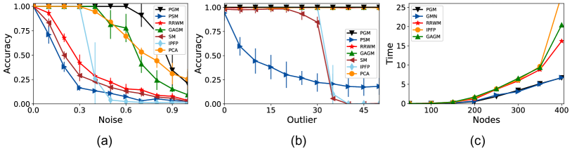
The set the experiment as follows: We generate a reference graph with nodes, and randomly generated an edge between any node pair with a probability . Each node in the reference graph is associated with an feature vector uniformly drawn from with . We duplicate the reference graph as a new graph preserving the same topology but we modify the feature vectors. Then, we set nodes as inliers and nodes as outliers. An inlier node means it has a matching in the other graph, while an outlier has no correspondence. In , the feature vector of an inlier node is perturbed with an additive i.i.d. Gaussian noise with zero mean and variance from its counterpart in , and for the outlier nodes, we generated a new i.i.d. feature vector following the same uniform distribution.
We construct the affinity matrix for all tested methods except PCA by setting the pairwise potential (edge affinity) as if and , and otherwise, where , and dropping the unary potential (node affinity). Permutation based intra-graph affinity (PCA) is based on the learnable graph neural network model. We train PCA with 2000 graph pairs for each task with the best parameter setting. Then, we fix the model, and transfer to other parameter setting.
Analysis robustness to noise.
We vary the noise level from 0.0 to 2.0, with other parameters fixed as , and . The results are shown in Figure 1(a).
Analysis the accuracy under different settings.
We change the number of outliers from to with , and being fixed. The results are presented in Figure 1(b).
In both experiments, our PGM outperforms all other baseline matching algorithms. We also note that the generalization performance of PCA [33] is also satisfactory, but it requires additional samples to train the model. On the other hand, the spectrum method, the base GM solver of GMN [36] does not work well. This is our initial motivation for exploring different differentiable module to seeking a better learning based GM method.
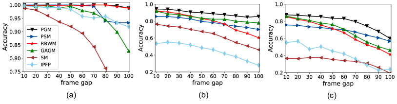
6.2.2 CMU House Sequence
The CMU House Sequence dataset contains totally 111 images of a house. Each image has 30 labeled landmarks. We build graphs by using these landmarks as nodes and adopting Delaunay triangulation to connect them. For all algorithms, affinity matrix is computed as , where means the distance between features and of two node from the same graph. We report the final average matching accuracy in Figure 2(a), 2(b) and 2(c) under different ratio settings of inliers-vs-outliers: 30:30, 25:30, 20:30. Our PGM achieves the best performance. Because the dataset is very small, grapg neural network based PCA cannot work here. Since the whole dataset too small to train PCA [33], we does not add this method into comparison.
6.3 Deep Feature Matching
The second group of experiments aims to test the compatibility of PGM and deep neural networks on the real-life PASCAL VOC dataset [14, 2]. The dataset has 20 classes of instances and 7,020 annotated images for training and 1,682 for testing. Berkeley’s annotations provide labeled keypoint locations [2].
6.3.1 PASCAL VOC Keypoint
The graph is built by setting those keypoints as nodes and then using Delaunay triangulation to introduce edges to connect landmarks. We use the feature from conv4-2 and conv5-1 layer of VGG-16 for all all situations [36][33]. Note that the width and height of feature map generated by VGG-16 is smaller than the given image, we cannot get the node features at precise location on the image level. Therefore, we use the bilinear interpolation to approximately recover the node feature of the given landmark pixel in the image. Similar technique is also used in [33, 36].
We compared with our DPGM method with two recent learning-based methods GMN [36], and PCA [33]. In addition, we also implement RRWM, GAGM and PSM as a differentiable module for comparison.
The results are listed in Table 1. We classify the test models into two category. The first model in the first category does not deploy any graph convolution network. Thus, there is no additional parameter other than those in the feature extractor. The second category attached a graph convolution network (GCN) after the feature extractor. The experiments in both category shows that the model with DPGM module performs best. Furthermore, we find the PGM without GCN outperforms the PCA, where the latter involves much more parameters the the former.
| method | aero | bike | bird | boat | bottle | bus | car | cat | chair | cow | table | dog | horse | mbike | person | plant | sheep | sofa | train | tv | mean |
|---|---|---|---|---|---|---|---|---|---|---|---|---|---|---|---|---|---|---|---|---|---|
| GMN | 31.9 | 47.2 | 51.9 | 40.8 | 68.7 | 72.2 | 53.6 | 52.8 | 34.6 | 48.6 | 72.3 | 47.7 | 54.8 | 51.0 | 38.6 | 75.1 | 49.5 | 45.0 | 83.0 | 86.3 | 55.3 |
| RRWM | 11.3 | 10.0 | 16.7 | 20.3 | 12.2 | 21.0 | 18.9 | 11.1 | 11.8 | 9.3 | 22.9 | 10.6 | 10.8 | 13.6 | 9.0 | 24.4 | 15.4 | 16.3 | 29.5 | 23.9 | 15.9 |
| GAGM | 16.4 | 18.9 | 20.1 | 27.2 | 18.2 | 25.4 | 23.5 | 15.7 | 19.7 | 14.1 | 21.5 | 15.7 | 13.7 | 19.6 | 11.7 | 36.7 | 21.1 | 18.0 | 37.4 | 36.7 | 21.6 |
| PSM | 12.8 | 12.6 | 17.9 | 24.2 | 20.8 | 37.9 | 27.2 | 12.8 | 21.25 | 14.9 | 19.9 | 13.6 | 14.6 | 16.1 | 11.8 | 24.7 | 18.0 | 21.3 | 53.6 | 42.91 | 21.9 |
| PGM | 45.6 | 60.6 | 52.79 | 50.3 | 76.3 | 81.1 | 69.6 | 63.5 | 42.7 | 59.3 | 83.5 | 58.1 | 66.4 | 59.8 | 43.6 | 81.8 | 64.9 | 56.3 | 85.5 | 89.4 | 64.6 |
| 40.9 | 55.0 | 65.8 | 47.9 | 76.9 | 77.9 | 63.5 | 67.4 | 33.7 | 65.5 | 63.6 | 61.3 | 68.9 | 62.8 | 44.9 | 77.5 | 67.4 | 57.5 | 86.7 | 90.9 | 63.8 | |
| 49.7 | 64.8 | 57.3 | 57.1 | 78.4 | 81.2 | 66.3 | 69.6 | 45.2 | 63.4 | 64.2 | 63.5 | 67.9 | 62.0 | 46.8 | 85.5 | 70.7 | 58.1 | 88.9 | 89.9 | 66.58 |
7 Conclusion
This paper has proposed a novel graph matching algorithm named as proximal graph matching (PGM). By introducing a proximal operator, PGM relax and decompose the original matching formula into a sequence of convex optimization objectives. By solving those convex sub-problems, PGM constructs a differentiable map from the node and edge affinity matrix to the prediction of node correspondence. Comparison experiments show that PGM outperforms existing graph matching algorithms on diverse datasets such as synthetic data, CMU House and PASCAL VOC. which operation matters for deep feature matching is also thoroughly studied. We draw a conclusion from those experiments that, for deep feature matching, the node affinity is important. A good graph matching should help the deep model to be fully trained and introduce appropriate additional correction.
References
- [1] Berg, A.C., Berg, T.L., Malik, J.: Shape matching and object recognition using low distortion correspondences. In: 2005 IEEE Computer Society Conference on Computer Vision and Pattern Recognition (CVPR’05). vol. 1, pp. 26–33 vol. 1 (June 2005)
- [2] Bourdev, L., Malik, J.: Poselets: Body part detectors trained using 3d human pose annotations. In: 2009 IEEE 12th International Conference on Computer Vision. pp. 1365–1372 (Sep 2009). https://doi.org/10.1109/ICCV.2009.5459303
- [3] Brendel, W., Todorovic, S.: Learning spatiotemporal graphs of human activities. In: International Conference on Computer Vision. pp. 778–785 (Nov 2011)
- [4] Burkard, R.E., Çela, E., Pardalos, P.M., Pitsoulis, L.S.: The Quadratic Assignment Problem, pp. 1713–1809. Springer (1998)
- [5] Caelli, T., Kosinov, S.: An eigenspace projection clustering method for inexact graph matching. IEEE Transactions on Pattern Analysis and Machine Intelligence 26(4), 515–519 (April 2004). https://doi.org/10.1109/TPAMI.2004.1265866
- [6] Caelli, T., Caetano, T.: Graphical models for graph matching: Approximate models and optimal algorithms. Pattern Recognition Letters 26(3), 339 – 346 (2005). https://doi.org/https://doi.org/10.1016/j.patrec.2004.10.022, in Memoriam: Azriel Rosenfeld
- [7] Caetano, T.S., McAuley, J.J., Cheng, L., Le, Q.V., Smola, A.J.: Learning graph matching. IEEE Transactions on Pattern Analysis and Machine Intelligence 31(6), 1048–1058 (June 2009). https://doi.org/10.1109/TPAMI.2009.28
- [8] Carcassoni, M., Hancock, E.R.: Spectral correspondence for point pattern matching. Pattern Recognition 36(1), 193 – 204 (2003). https://doi.org/https://doi.org/10.1016/S0031-3203(02)00054-7
- [9] Cho, M., Lee, J., Lee, K.M.: Reweighted random walks for graph matching. In: Daniilidis, K., Maragos, P., Paragios, N. (eds.) Computer Vision – ECCV 2010. pp. 492–505. Springer Berlin Heidelberg, Berlin, Heidelberg (2010)
- [10] Christmas, W.J., Kittler, J., Petrou, M.: Structural matching in computer vision using probabilistic relaxation. IEEE Transactions on Pattern Analysis and Machine Intelligence 17(8), 749–764 (Aug 1995). https://doi.org/10.1109/34.400565
- [11] Cour, T., Srinivasan, P., Shi, J.: Balanced graph matching. In: Schölkopf, B., Platt, J.C., Hoffman, T. (eds.) Advances in Neural Information Processing Systems 19, pp. 313–320. MIT Press (2007)
- [12] Egozi, A., Keller, Y., Guterman, H.: A probabilistic approach to spectral graph matching. IEEE Transactions on Pattern Analysis and Machine Intelligence 35(1), 18–27 (Jan 2013). https://doi.org/10.1109/TPAMI.2012.51
- [13] Elmsallati, A., Clark, C., Kalita, J.: Global alignment of protein-protein interaction networks: A survey. IEEE/ACM Transactions on Computational Biology and Bioinformatics 13(4), 689–705 (July 2016). https://doi.org/10.1109/TCBB.2015.2474391
- [14] Everingham, M., Van Gool, L., Williams, C.K.I., Winn, J., Zisserman, A.: Pascal visual object classes challenge 2011 (voc2011) complete dataset
- [15] Gaur, U., Zhu, Y., Song, B., Roy-Chowdhury, A.: A “string of feature graphs” model for recognition of complex activities in natural videos. In: 2011 International Conference on Computer Vision. pp. 2595–2602 (Nov 2011)
- [16] Gold, S., Rangarajan, A.: A graduated assignment algorithm for graph matching. IEEE Transactions on Pattern Analysis and Machine Intelligence 18(4), 377–388 (April 1996). https://doi.org/10.1109/34.491619
- [17] Gomila, C., Meyer, F.: Graph-based object tracking. In: Proceedings 2003 International Conference on Image Processing (Cat. No.03CH37429). vol. 2, pp. II–41 (Sep 2003). https://doi.org/10.1109/ICIP.2003.1246611
- [18] Ham, B., Cho, M., Schmid, C., Ponce, J.: Proposal flow: Semantic correspondences from object proposals. IEEE Transactions on Pattern Analysis and Machine Intelligence 40(7), 1711–1725 (July 2018). https://doi.org/10.1109/TPAMI.2017.2724510
- [19] Hancock, E., Wilson, R.C.: Graph-based methods for vision: A yorkist manifesto. In: Caelli, T., Amin, A., Duin, R.P.W., de Ridder, D., Kamel, M. (eds.) Structural, Syntactic, and Statistical Pattern Recognition. pp. 31–46. Springer Berlin Heidelberg, Berlin, Heidelberg (2002)
- [20] Huet, B., Hancock, E.R.: Shape recognition from large image libraries by inexact graph matching. Pattern Recognition Letters 20(11), 1259 – 1269 (1999). https://doi.org/https://doi.org/10.1016/S0167-8655(99)00093-8
- [21] Hwann-Tzong Chen, Horng-Horng Lin, Tyng-Luh Liu: Multi-object tracking using dynamical graph matching. In: Proceedings of the 2001 IEEE Computer Society Conference on Computer Vision and Pattern Recognition. CVPR 2001. vol. 2, pp. II–II (Dec 2001). https://doi.org/10.1109/CVPR.2001.990962
- [22] Khan, M.E.E., Baque, P., Fleuret, F., Fua, P.: Kullback-leibler proximal variational inference. In: Cortes, C., Lawrence, N.D., Lee, D.D., Sugiyama, M., Garnett, R. (eds.) Advances in Neural Information Processing Systems 28, pp. 3402–3410. Curran Associates, Inc. (2015), http://papers.nips.cc/paper/5895-kullback-leibler-proximal-variational-inference.pdf
- [23] Koopmans, T.C., Beckmann, M.: Assignment problems and the location of economic activities. Econometrica 25(1), 53–76 (1957)
- [24] Leordeanu, M., Hebert, M.: A spectral technique for correspondence problems using pairwise constraints. In: Tenth IEEE International Conference on Computer Vision (ICCV’05) Volume 1. vol. 2, pp. 1482–1489 Vol. 2 (Oct 2005). https://doi.org/10.1109/ICCV.2005.20
- [25] Leordeanu, M., Hebert, M., Sukthankar, R.: An integer projected fixed point method for graph matching and map inference. In: Bengio, Y., Schuurmans, D., Lafferty, J.D., Williams, C.K.I., Culotta, A. (eds.) Advances in Neural Information Processing Systems 22, pp. 1114–1122. Curran Associates, Inc. (2009)
- [26] Li: A markov random field model for object matching under contextual constraints. In: 1994 Proceedings of IEEE Conference on Computer Vision and Pattern Recognition. pp. 866–869 (June 1994). https://doi.org/10.1109/CVPR.1994.323915
- [27] Long, J., Zhang, N., Darrell, T.: Do convnets learn correspondence? In: Proceedings of the 27th International Conference on Neural Information Processing Systems - Volume 1. p. 1601–1609. NIPS’14, MIT Press, Cambridge, MA, USA (2014)
- [28] Shapiro, L.S., Brady, J.M.: Feature-based correspondence: an eigenvector approach. Image and Vision Computing 10(5), 283 – 288 (1992). https://doi.org/https://doi.org/10.1016/0262-8856(92)90043-3, bMVC 1991
- [29] Siddiqi, K., Shokoufandeh, A., Dickenson, S.J., Zucker, S.W.: Shock graphs and shape matching. In: Sixth International Conference on Computer Vision (IEEE Cat. No.98CH36271). pp. 222–229 (Jan 1998). https://doi.org/10.1109/ICCV.1998.710722
- [30] Simonyan, K., Zisserman, A.: Very deep convolutional networks for large-scale image recognition. In: International Conference on Learning Representations (2015)
- [31] Sinkhorn, R., Knopp, P.: Concerning nonnegative matrices and doubly stochastic matrices. Pacific J. Math. 21(2), 343–348 (1967)
- [32] Wang, H., Hancock, E.R.: A kernel view of spectral point pattern matching. In: Fred, A., Caelli, T.M., Duin, R.P.W., Campilho, A.C., de Ridder, D. (eds.) Structural, Syntactic, and Statistical Pattern Recognition. pp. 361–369. Springer Berlin Heidelberg, Berlin, Heidelberg (2004)
- [33] Wang, R., Yan, J., Yang, X.: Learning combinatorial embedding networks for deep graph matching. In: The IEEE International Conference on Computer Vision (ICCV) (October 2019)
- [34] Wang, T., Ling, H.: Gracker: A graph-based planar object tracker. IEEE Transactions on Pattern Analysis and Machine Intelligence 40(6), 1494–1501 (June 2018). https://doi.org/10.1109/TPAMI.2017.2716350
- [35] Wilson, R.C., Hancock, E.R.: Structural matching by discrete relaxation. IEEE Trans. Pattern Anal. Mach. Intell. 19(6), 634–648 (Jun 1997). https://doi.org/10.1109/34.601251
- [36] Zanfir, A., Sminchisescu, C.: Deep learning of graph matching. In: 2018 IEEE/CVF Conference on Computer Vision and Pattern Recognition. pp. 2684–2693 (June 2018). https://doi.org/10.1109/CVPR.2018.00284