Multi-Level Additive Modeling for
Structured Non-IID Federated Learning
Abstract
The primary challenge in Federated Learning (FL) is to model non-IID distributions across clients, whose fine-grained structure is important to improve knowledge sharing. For example, some knowledge is globally shared across all clients, some is only transferable within a subgroup of clients, and some are client-specific. To capture and exploit this structure, we train models organized in a multi-level structure, called “Multi-level Additive Models (MAM)”, for better knowledge-sharing across heterogeneous clients and their personalization. In federated MAM (FeMAM), each client is assigned to at most one model per level and its personalized prediction sums up the outputs of models assigned to it across all levels. For the top level, FeMAM trains one global model shared by all clients as FedAvg. For every mid-level, it learns multiple models each assigned to a subgroup of clients, as clustered FL. Every bottom-level model is trained for one client only. In the training objective, each model aims to minimize the residual of the additive predictions by the other models assigned to each client. To approximate the arbitrary structure of non-IID across clients, FeMAM introduces more flexibility and adaptivity to FL by incrementally adding new models to the prediction of each client and reassigning another if necessary, automatically optimizing the knowledge-sharing structure. Extensive experiments show that FeMAM surpasses existing clustered FL and personalized FL methods in various non-IID settings. Our code is available at https://github.com/shutong043/FeMAM.
1 Introduction
Federated Learning (FL) emerges as a paradigm shift in distributed machine learning, allowing many clients to collectively enhance centralized models without disclosing their private datasets kairouz2021advances ; konevcny2016federated ; li2020federatedsummary ; yang2019federated ; yu2023federated ; charles2024towards . In practice, real-world data across different users are non-identically independently distributed (non-IID) zhao2018federated and often exhibit fine-grained structures. Understanding non-IID across clients is a crucial factor to design and choose FL methods in real applications. To design an FL method, the hidden structure of knowledge sharing preserves various non-IIDness across clients. In the application of FL systems, the system architecture must estimate the structured Non-IID based on application scenarios including user behaviour analysis and hierarchical relation among clients.
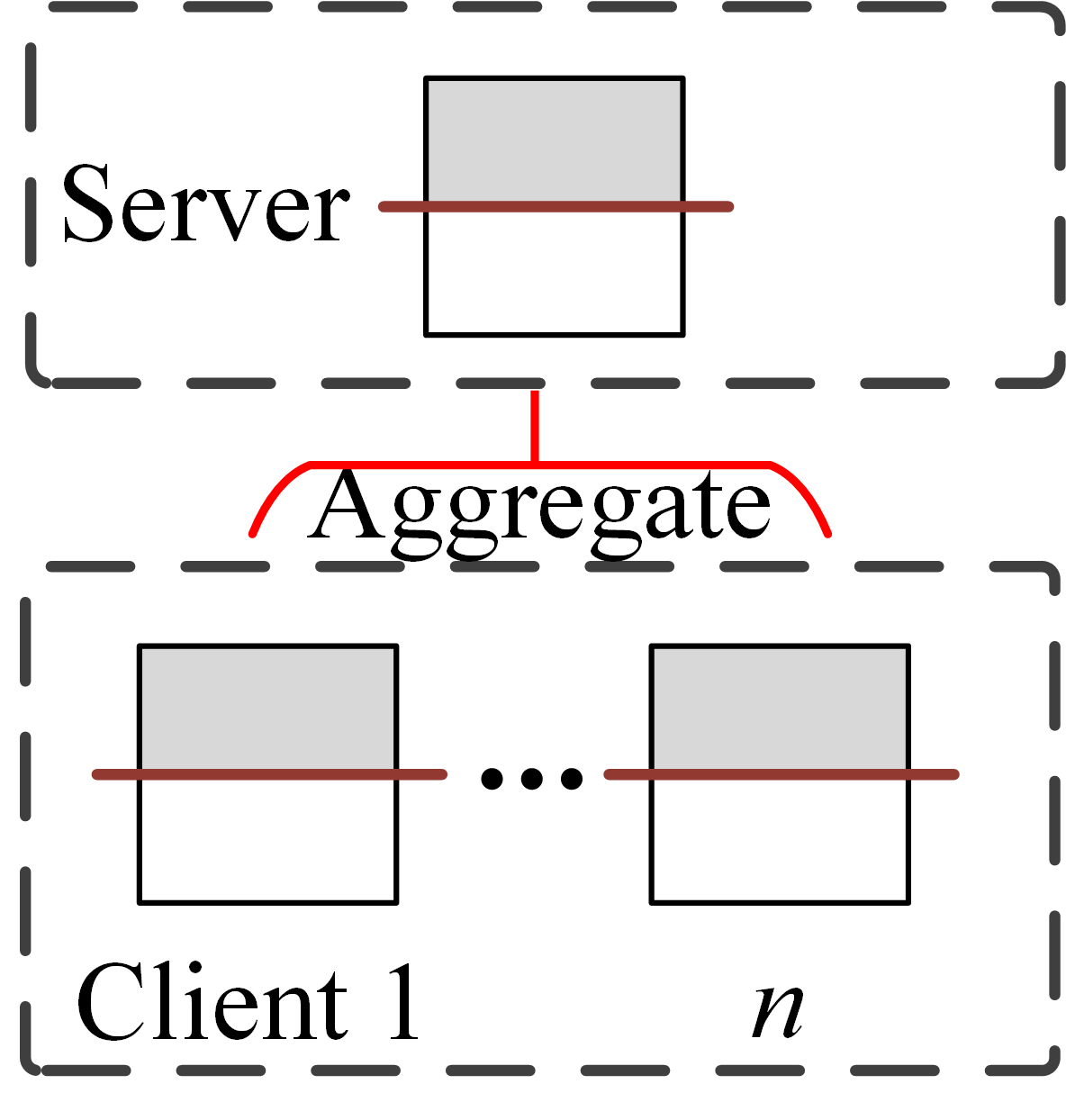
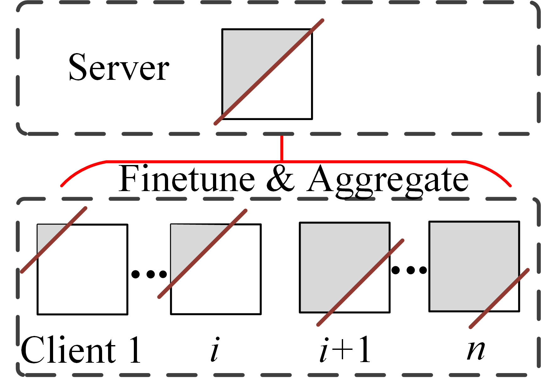
The structure of Non-IID, as illustrated in Figure 1, can be categorized into four types. 1) IID and Slight Non-IID (proposed by FedAvg), which can be solved using a global model mcmahan2017communication ; karimireddy2020scaffold ; li2020federated to aggregate all shared knowledge across clients. 2) Cluster-wise Non-IID to be solved by clustered FL sattler2020clustered ; ghosh2020efficient ; xie2021multi ; ma2022personalized that groups clients into several non-overlapping clusters and optimize one model for each cluster. 3) Client-wise Non-IID to be solved by personalized FL shamsian2021personalized ; li2021ditto ; t2020personalized ; agarwal2020federated ; li2021fedbn ; zhang2023dual ; tan2023federated that assumes knowledge across clients are distinct and optimizes each model in a client-wise manner; 4) Multi-level Non-IID to be studied by this paper that aims to explore a fine-grained knowledge-sharing structure to approximate arbitrary structure of Non-IID including the mentioned three types of Non-IID and others.

Intuitively, multi-level non-IID in FL indicates sharing knowledge in multiple granularity at various levels. For example, some higher-level concepts are shared across all clients, some lower-level concepts and patterns can only be shared among a small group of clients but contradictory between different groups, and some characteristics are client-specific. Moreover, different groups of clients may share partial but not all concepts or features. However, such a rich structure has not been studied directly in existing FL approaches.
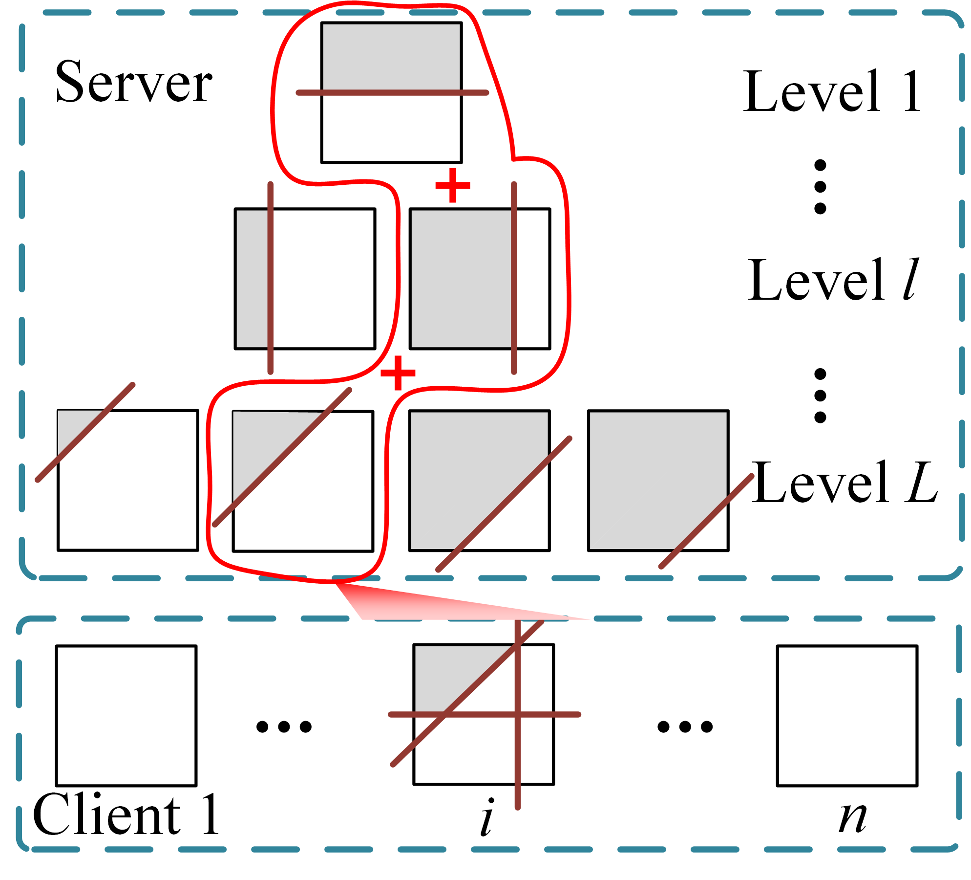
In this paper, we proposed Multi-level Additive Modeling (MAM), which provides a natural solution to the above multi-level non-IID problem with a fine-grained knowledge-sharing structure in an FL system. MAM jointly learns a multi-level structure and the shared models at each level. It embodies the model personalization for each client- by adding outputs from multiple shared models from different levels. At each level, only one shared model will be assigned to the client in the top-down manner. Specifically, an -level MAM produces a personalized for client- as , where is the index of the model assigned to client- in level- and the sequence is highlighted as a pathway of the red color in Fig. 1(d).
We develop an efficient and adaptive federated learning algorithm FeMAM to jointly learn a multi-level structure and many shared models in a top-down manner. FeMAM is adaptive in determining clients participating in the knowledge sharing at each level. The top-down additive modeling in FeMAM allows a client to stop joining the current level if the latest model achieves a sufficiently small validation loss. Hence, can vary across different clients, and client- with a simpler data distribution may have a smaller than others, leading to a less complex personalized model .
Our main contributions can be summarized below:
-
•
The first to propose a Multi-level Non-IID setting in Federated Learning.
-
•
We proposed a novel Multi-Level Additive Modeling (MAM) to effectively integrate multiple shared models across levels.
-
•
We developed a new learning algorithm FeMAM to incrementally add new models to clients during training, enabling joint learning of models and structure.
-
•
We provided convergence analysis to support the proposed method.
-
•
Experiments on a variety of non-IID settings demonstrated that our method surpasses Cluster FL and Personalize FL methods by a large margin.
2 Related Works
Global FL. The concept of federated learning was first introduced in FedAvg mcmahan2017communication , where weight averaging of local objectives is optimized across all clients. There are methods that speed up the convergence of FedAvg li2020federated ; karimireddy2020scaffold , as well as analyses of FedAvg’s convergence under non-IID data li2019convergence . FedAvg often serves as the foundation for other methods, providing global information for personalized models or a warm start for cluster models. In our method, we also utilize FedAvg to provide global information.
Clustered FL. Clustered Federated Learning assumes clients share knowledge within several clusters, and aggregates inside each cluster separately. For example, CFL sattler2020clustered separates each cluster into two distinct sub-clusters when the gradient divergence is significant. There are methods that utilize various clustering techniques. xie2021multi uses Expectation Maximization (EM) optimization, while briggs2020federated employs hierarchical clustering. ma2022convergence provides a convergence analysis of the clustering algorithm. While the above methods assign clients to clusters with clustering algorithms, IFCAghosh2020efficient assigns clients with the clusters which can achieve the best local performance. Recently, bao2023optimizing employed a two-phase approach to optimize the clustering and federated learning loss separately.
Personalized FL. Personalized FL tan2022toward ; wu2023personalized ; baek2023personalized ; xu2023personalized ; yao2022fedgcn ; jiang2022test aims to learn many optimal local models simultaneously. pFedMe t2020personalized uses Moreau envelopes as clients’ regularized loss functions, decoupling personalized model optimization from the global model. Ditto li2021ditto optimizes the global and local models in a bi-level manner and incorporates a regularization term to relate the two tasks. Additionally, there are methods that personalize parts of the models. In tan2021fedproto , clients share personalized prototypes for each class. collins2021exploiting personalizes the head layers for each model, while li2021fedbn personalizes the batch normalization layer.
Additive Modeling. The concept was first introduced in agarwal2020federated , where the local model is treated as a residual to the global model. ma2023structured applies additive modelling on clustered FL by integrating a global model and cluster models. In li2023federated , local models are added to global models, allowing the local model to complement features that the global model lacks. However, current methods typically employ a fixed two-level additive structure, which limits their capacity to approximate arbitrary structures of Non-IID across clients.
3 Methodology
3.1 Problem Formulation
Personalized FL Following the general definition of FL, the FL system consists of clients and the -th client’s local dataset is {, }. Each client’s learning objective is to minimize the loss function . In personalized FL, we assume the -th client’s function is embodied by a neural network-based model which is parameterized by . The learning objective of the FL system is:
| (1) |
where the is the number of instances in the local dataset on the -th client, and is the total number of instances across all clients.
Local Objective in FeMAM In the proposed FeMAM, the -th client’s local personalized model is implemented by taking number of shared models, thus . Additive modeling is applied to sum up these models’ outputs to form a final prediction. Below is the learning objective of FeMAM:
| (2) |
Global Objective in FeMAM In FeMAM, the shared model is embodied by an level of model sets that can capture shared knowledge in a fine-grained manner. More specifically, the -th level of shared knowledge is captured by a set of functions parameterized by . To match the assignment of multi-level shared models to clients, we define a level-wise mapping function that maps the assignment of the set of local models to its corresponding in different levels. Accordingly, FeMAM’s learning objective is as below:
| (3) |
where we replace with in Eq. (2).
3.2 Structure of Multi-Level Additive Modeling
It is impractical to optimize the Eq. (3) with a complex multi-level structure of shared model set . To simplify the problem, we decompose the multi-level structure into three components: (i) One globally shared model that includes Level , (ii) Cluster shared models that include Level to , and (iii) Personalized models that include Level . The corresponding number of models per level is defined as . The details of the three components are illustrated below.
One Global Model at Level . A single global model in the first level will be shared globally with all clients. It is compatible with FedAvg by assuming one global model can preserve the universal shared knowledge. Thus, we have at level of Eq. (3) . Local models set across all clients are assigned by one global model .
Cluster Models at Level to . For the levels from 2 to the , the number of shared models per level is a set of flexible numbers to capture the clustered shared knowledge with unknown hidden structures. Specifically, a clustering algorithm is applied per level to learn the fine-grained shared knowledge by aggregating similar clients, thus the implementation of these levels will be compatible with clustered FL. We have , where . Following xie2021multi , we apply Stochastic Expectation Maximization optimization to each level of cluster. The mapping function is obtained by the nearest-center criterion in the K-means algorithm, i.e.,
| (4) |
Personalized Models at Level . The shared models on the last level are virtual models on the server because they will be stored on each client by taking the form of a client-specific model . Specifically, one level of local training is applied to the last level of Eq. (3) to capture the client-specific information. Then we have . Local models set are kept and fine-tuned on their own clients. These models are compatible with personalized FL methods that believe each client can use a unique personalized model to capture client-specific knowledge.
Refined Objective Function In summary, we can rewrite the objective function in Eq. (3) to a new form. Specifically, we will use FedAvg to level , apply Eq. (4) to levels , and conduct local fine-tuning to level . The refined learning objective is as below:
| (5) |
Eq. (5) concrete Eq. (3) with the specific form of the mapping function, and represents .
3.3 Level-wise Optimization
Given the multi-level structure, the level-wise alternating minimization schema is proposed to efficiently solve the objective function in Eq. (5). For mapping function at each level, we define its inverse function as . The general level-wise aggregation and broadcast operation is as below:
| (6) |
| (7) |
where is the set of local clients that assigned to. By settings and to specific forms in Eq. (6) and Eq. (7) respectively, i.e., for global level, for cluster level, and for personalized level, we obtain the broadcast and aggregate operation at every level.
At local optimization, each client conduct a local learning-based gradient descent step in a level-wise manner. Each level of model is iteratively optimized while fixing other levels:
| (8) |
We provide the specific form of update steps at global, cluster and personalized levels in Appendix.
3.4 Practical Implementations of FeMAM
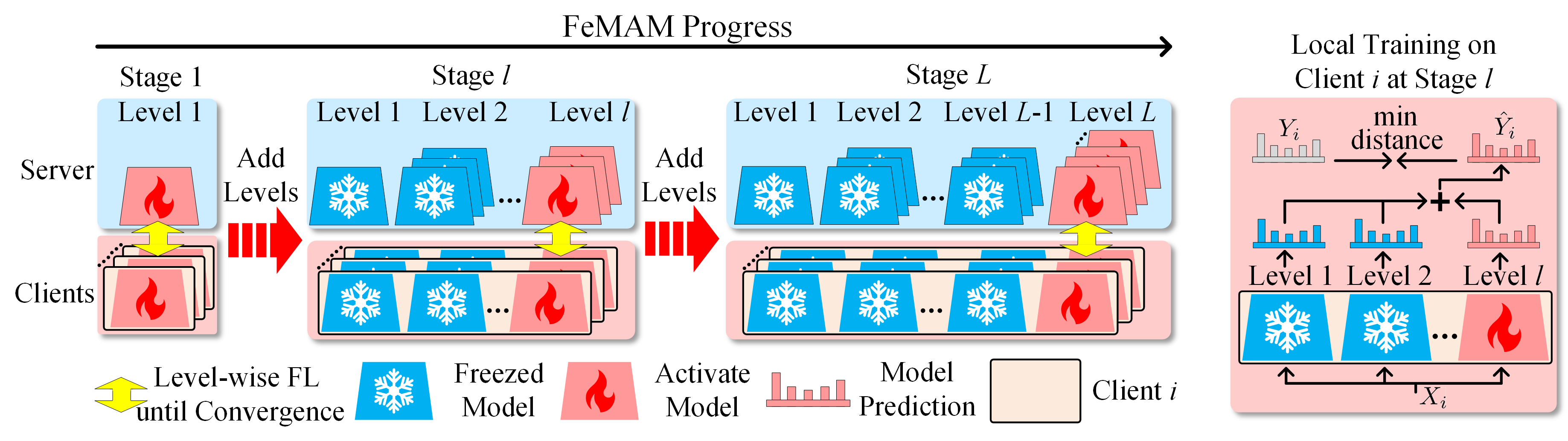
We give out the practical application of FeMAM based on the analytical results. These strategies aim to reduce the possible instability of training, speed up convergence, and improve performance. Fig. 2 illustrates the overall framework of the proposed FeMAM. We provide the learning algorithm of FeMAM in Algorithm 1 and the full algorithm is in Appendix.
Progressive Level Adding Based on the analytical results, all levels of models are randomly initialized and start training from the first round. In practice, such an operation is risky because each level has its own objective, and they will interfere with each other through additive modeling. We thus initialize FeMAM with FedAvg, i.e., the first level. As training proceeds, we add new models level by level gradually until FeMAM reaches the maximum length . New levels are added only when the current training stabilizes, i.e., when it converges.
Efficient Training with Subset of Levels Training all levels of models at every communication round is time costly. In practice, training with a subset of levels is good enough to achieve superior accuracy, and significantly accelerate the training process. Specifically, at each local training round, only the last level is optimized while all the previous levels of models are fixed. The previous models only act as an add-on prediction to the client’s prediction. As the level grows, the structure of converged models continues to grow until the maximum depth .
Model Pruning with Loss Reduction Orientation Due to non-IIDness, not all models at each level contribute to each client’s performance. After the latest level of models has converged, we check the validation loss on each client before and after adding the latest model. Models that only marginal reduce the validation loss by less than are removed:
| (9) |
where is the latest level. This straightforward strategy allows each client to select only beneficial models and results in distinct number models for each client. The system thus discovers a unique structure for each non-IID setting. In experiments we set .
With all the practical techniques mentioned above, FeMAM is communication-efficient, stable in training, and achieves high accuracy with acceptable increases in communication parameters and running time. For detailed cost analysis, please refer to Section A in the Appendix.
4 Convergence analysis
Eq. (5) can be decoupled into two components, the Expectation Maximization (EM) objective and the FL objective . For the EM objective , we bound its decreasing in arbitrary consecutive communication rounds conditioned on learning rate . For the FL objective , The update of levels can be decoupled into sum of update for each level, so each level can be bounded separately.
4.1 Convergence of Clustering Objective
Theorem 1.
(Convergence of clustering objective on cluster levels). Assume for each level at client , the expectation of the stochastic gradient is unbiased, and the L2 norm is bounded by a constant . Let be the local training epochs. Then for arbitrary communication round , converges when:
4.2 Convergence of FeMAM
Assumption 1.
(Compactness of mapping function). For arbitrary client at level , let . For clients in inverse mapping function , let the average gradient at level be . Then
We upper-bounded the gradient variance across clients in each inverse mapping function.
Theorem 2.
(Convergence of FeMAM). Assume for arbitrary level at client , local loss function is convex and Lipschitz Smooth. For arbitrary level , the variance of the stochastic gradient is bounded by . Then at level , local epoch and communication round , when
the EM loss function converges, and the FL loss function decreases monotonically, thus the FeMAM converges.
| Dataset | Non-IID Type | Metric | Local | FedAvg | FedAvg+ | PFedMe | Ditto | FeSEM | FeSEM+ | FeMAM |
|---|---|---|---|---|---|---|---|---|---|---|
| Tiny ImageNet | Cluster-wise | Accuracy | 15.570.03 | 24.870.80 | 36.740.09 | 38.760.31 | 37.120.70 | 41.200.25 | 31.600.42 | 46.800.35 |
| Macro-F1 | 10.420.17 | 12.630.49 | 32.970.23 | 34.870.45 | 33.740.80 | 37.820.21 | 26.720.61 | 43.290.34 | ||
| Client-wise | Accuracy | 28.930.21 | 24.330.34 | 45.850.13 | 44.730.54 | 47.080.16 | 22.340.79 | 44.930.34 | 60.460.35 | |
| Macro-F1 | 8.000.15 | 8.730.24 | 23.840.03 | 22.570.79 | 24.570.23 | 7.790.19 | 17.451.74 | 33.290.15 | ||
| Multi-level | Accuracy | 39.480.36 | 17.910.09 | 56.800.21 | 55.870.51 | 58.830.18 | 34.140.69 | 51.640.30 | 65.300.17 | |
| Macro-F1 | 28.990.43 | 4.490.07 | 52.330.56 | 50.250.62 | 51.820.53 | 19.100.67 | 44.930.34 | 60.460.35 | ||
| CIFAR-100 | Cluster-wise | Accuracy | 22.810.11 | 29.280.48 | 46.670.74 | 46.300.31 | 45.160.18 | 45.100.51 | 37.330.99 | 53.720.29 |
| Macro-F1 | 13.800.33 | 12.730.15 | 39.770.91 | 39.050.36 | 38.050.76 | 38.730.60 | 29.701.41 | 48.330.40 | ||
| Client-wise | Accuracy | 38.570.15 | 30.460.15 | 53.570.45 | 53.740.09 | 56.060.48 | 25.880.12 | 44.790.22 | 61.960.48 | |
| Macro-F1 | 11.900.11 | 11.530.08 | 29.490.41 | 28.680.20 | 30.710.34 | 9.420.18 | 18.040.24 | 36.410.70 | ||
| Multi-level | Accuracy | 28.670.33 | 25.080.30 | 49.730.32 | 51.850.17 | 51.730.39 | 41.480.59 | 44.380.17 | 61.860.32 | |
| Macro-F1 | 11.970.17 | 15.060.15 | 40.130.47 | 44.100.41 | 42.530.57 | 32.750.77 | 34.860.22 | 55.260.77 |
(Non-IID)
5 Experiments
5.1 Experimental Setup
Dataset and System Settings: We evaluate methods on two benchmark datasets: Tiny ImageNetLe2015TinyIV and CIFAR-100krizhevsky2009learning . We use a validation dataset to monitor the performance and select the checkpoint with the minimum evaluation error. The size of the validation set is set to be half of the original testing set. The number of clients is , and local training epochs is . Resnet- he2016deep is selected as the basic model.
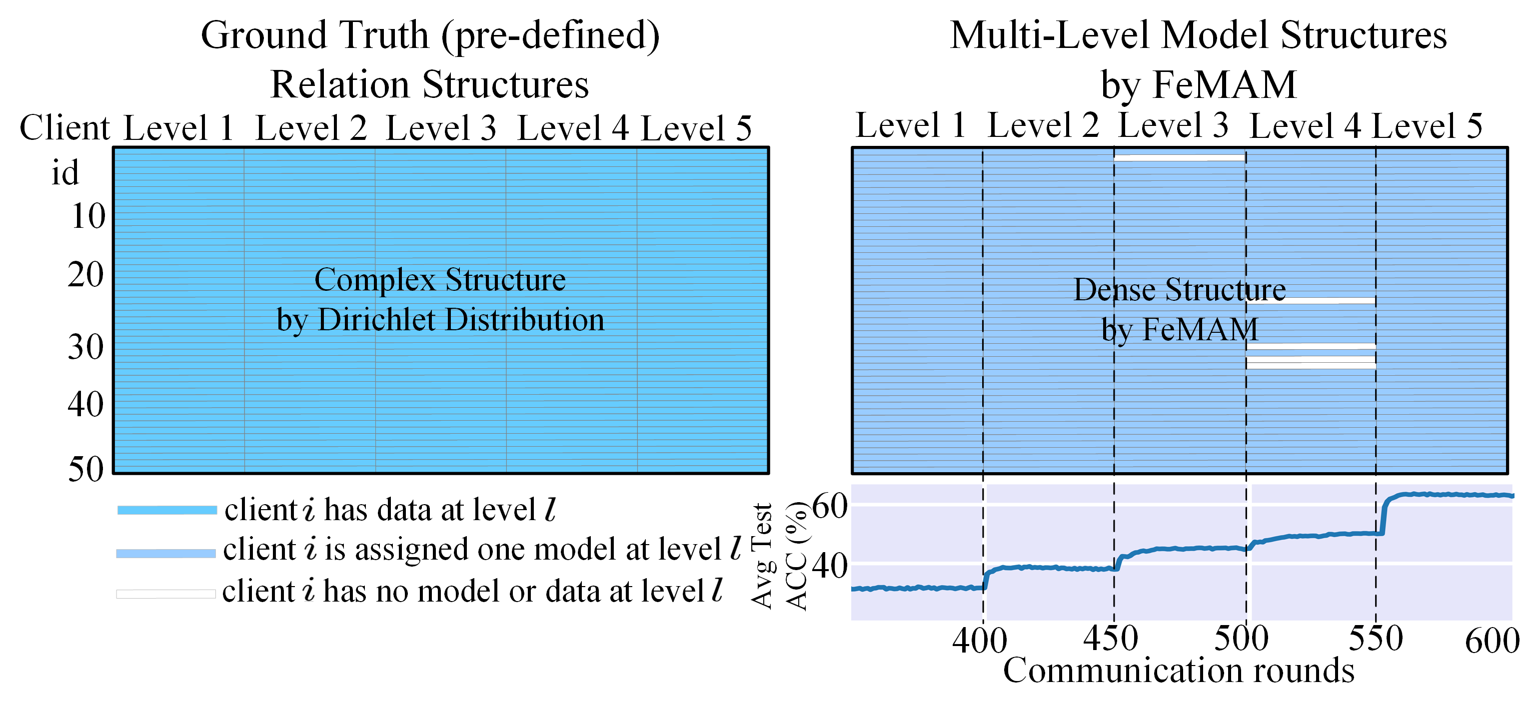
Mimic Non-IID Setting: We evaluate FeMAM on three types of non-IID settings that include distinguishable relational structures and irregular inherent structures.
(I) Cluster-wise Non-IID: A common setting for cluster FL. We split the dataset into several clusters to achieve distinct data distribution structures. For example, means clusters, each cluster with 30 classes. Different non-IIDness is achieved by varying the number of classes per cluster.
(II) Client-wise Non-IID: A general setting proposed by hsu2019measuring , popular in personalized FL. It partitions data with Dirichlet distribution, and uses concentration parameter to control the non-IIDness. We set to mimic a highly non-IID setting. The data structure is inherent due to randomness.
(III) Multi-level Non-IID: We build a non-IID-based relation among clients with multiple levels. The dataset is first split into several non-overlapping parts (levels) by class labels. We assign each level of data to clients by following the rules of cluster-wise partition. For example, means the dataset is split into three levels, and each level has , , number of clusters respectively. For more details on the structure, please refer to Appendix Table C.1.
Baselines: We consider popular methods comprehensively from 1) Global FL: FeAvgmcmahan2017communication and FedProxli2020federated ; 2) Clustered FL: FeSEMxie2021multi ; 3) Personalized FL: PFedMet2020personalized , FedRepcollins2021exploiting , Dittoli2021ditto , FedAvg+, FeSEM+ and Local. FedAvg+ and FeSEM+ denote an integration with personalized fine-tuning for 2 epochs. Local denotes to train the model use local data only.
FeMAM: The number of level is set to be , i.e., one global level, three clustered levels and one personalized level. The number of clusters is set to for all cluster levels. Threshold in Eq. (9) is set to be 0, which means we prune models that increase the validation loss. The communication rounds for the first level is set to and the subsequent levels will converge quickly in epochs.
5.2 Numerical Results
Table 1 shows compare FeMAM and other baselines in terms of the accuracy and macro-F1 score with mean (std) value of independent runs. The results suggest that:
Baselines only perform well on the desired non-IID. Clustered FL, i.e., FeSEM, performs well on cluster-wise non-IID and shows poor results on the client-wise non-IID. In contrast, personalized FL shows superior results on client-wise non-IID.
FeMAM outperforms baselines in all types of non-IID. FeMAM outperformed the comparative methods across their respective advantageous non-IID data distributions, from data distributions with specific structures (cluster-wise, fine-grained) to inherent structures (client-wise). The results demonstrate FeMAM’s generalization capability in various scenarios of FL applications.
5.3 Convergence Analysis
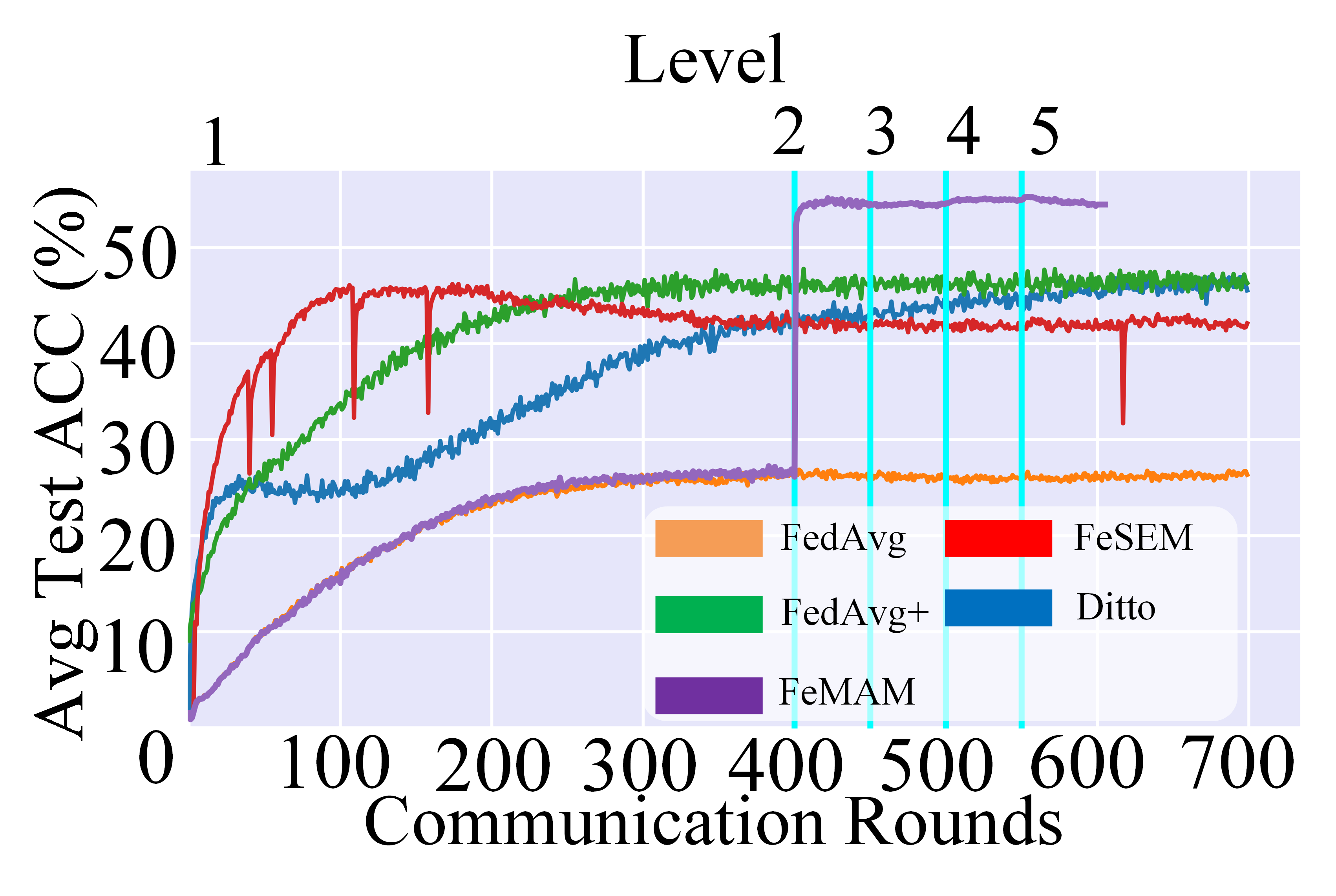
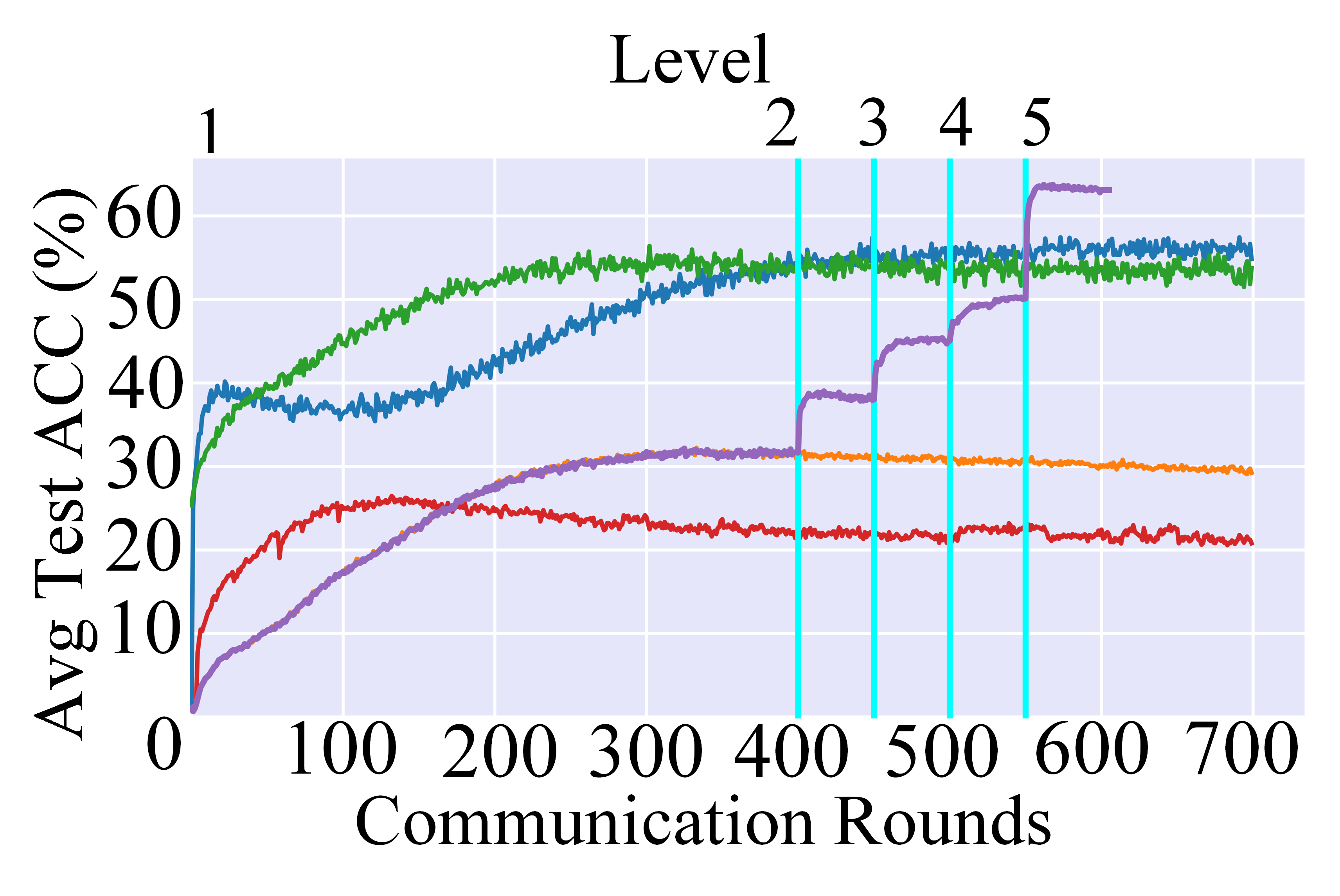
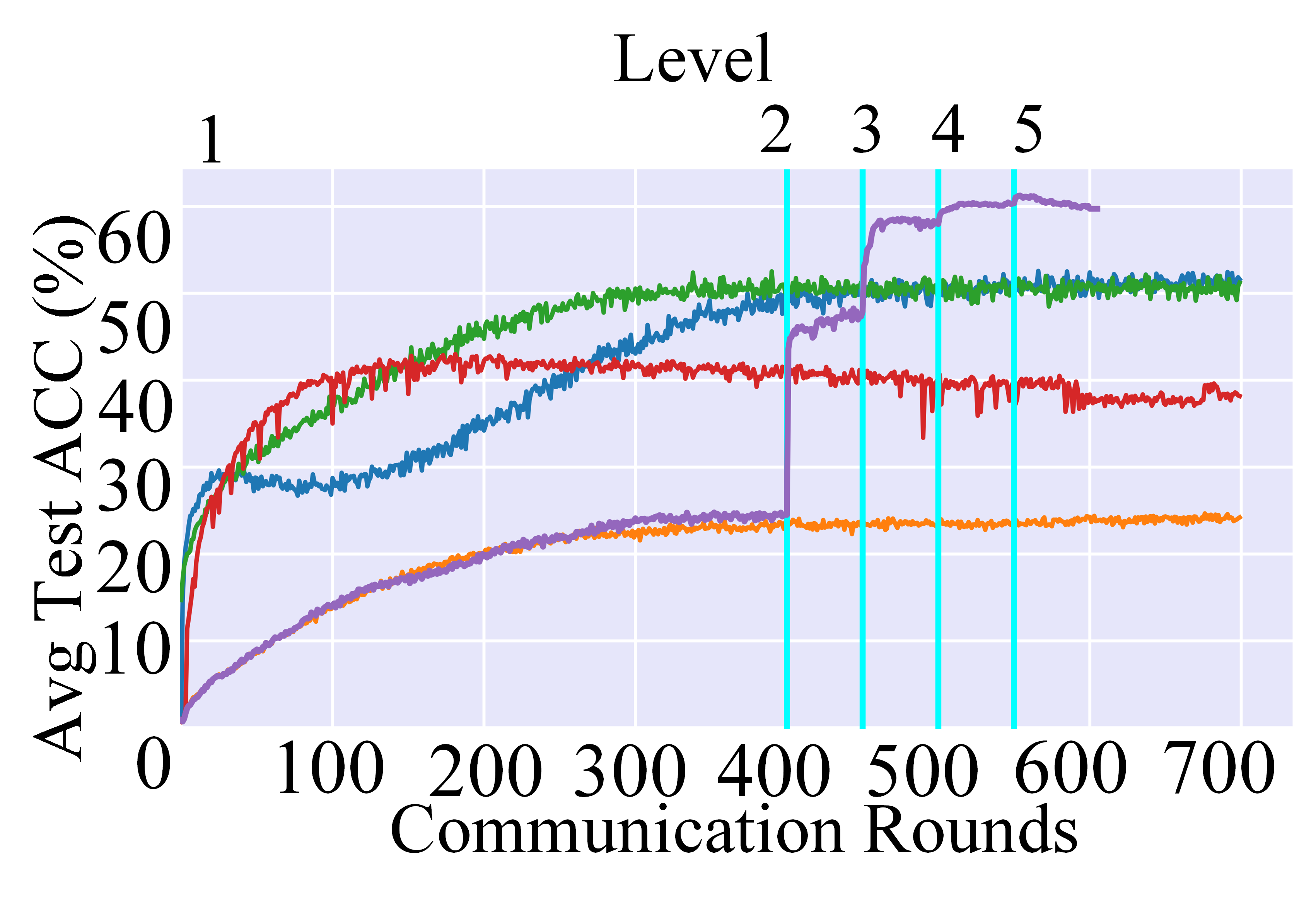
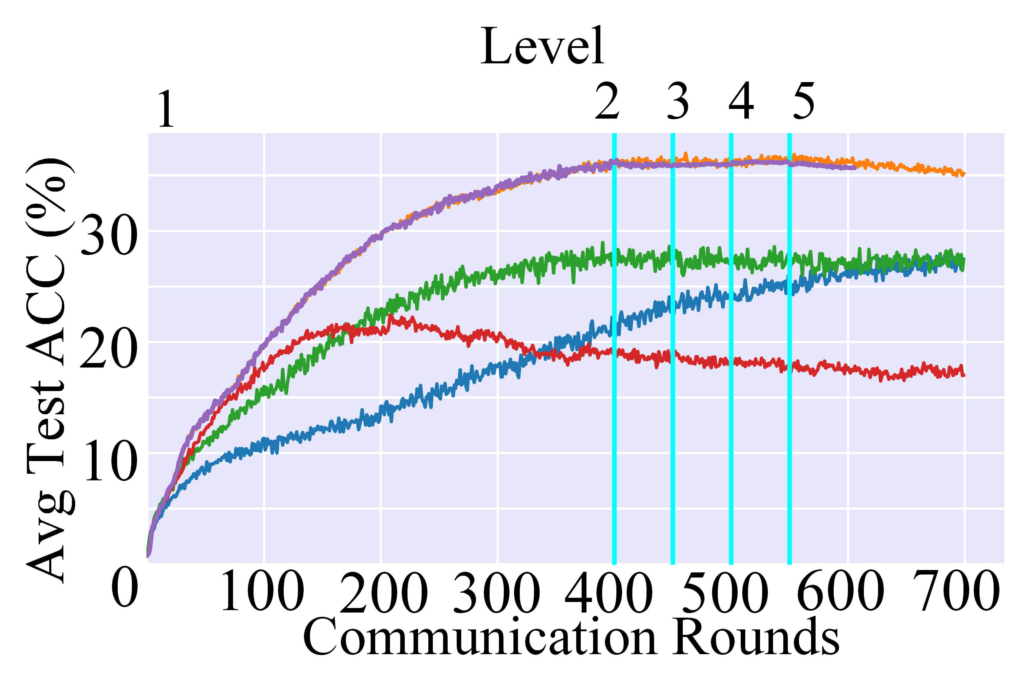
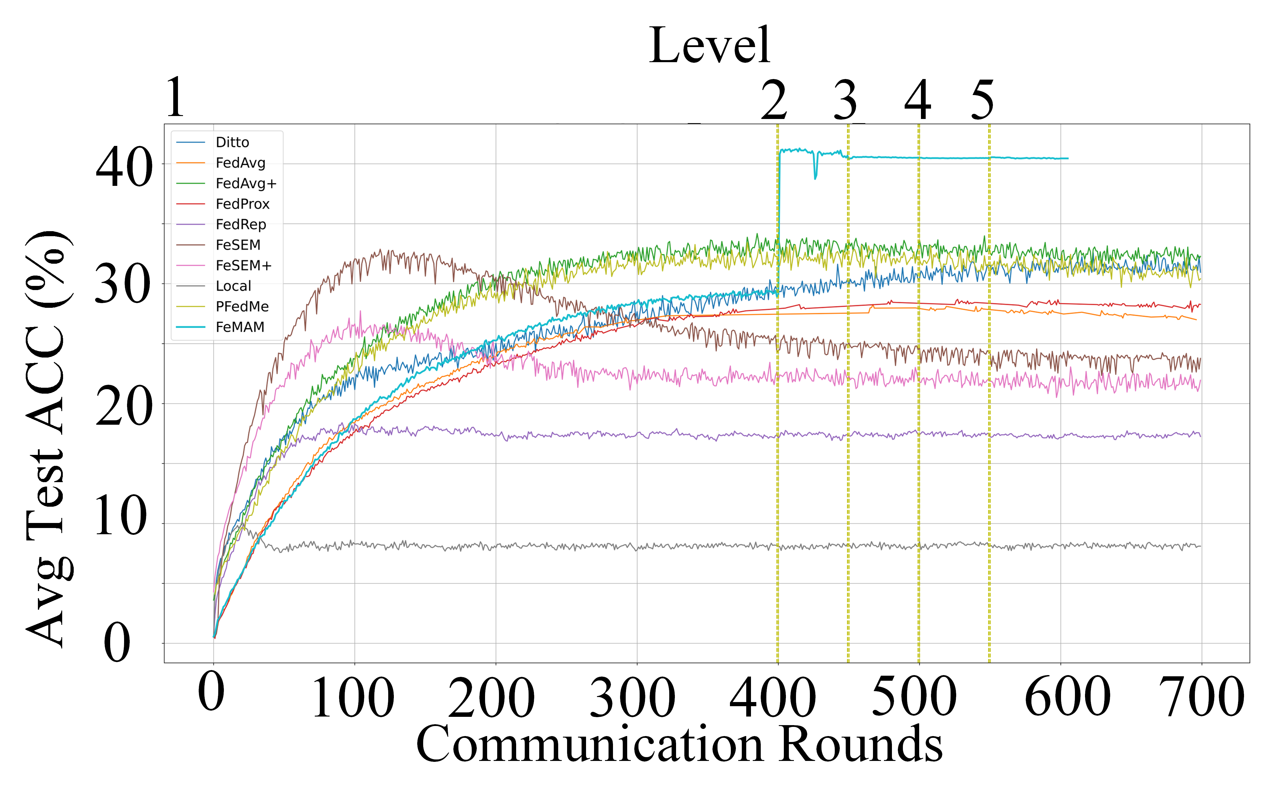
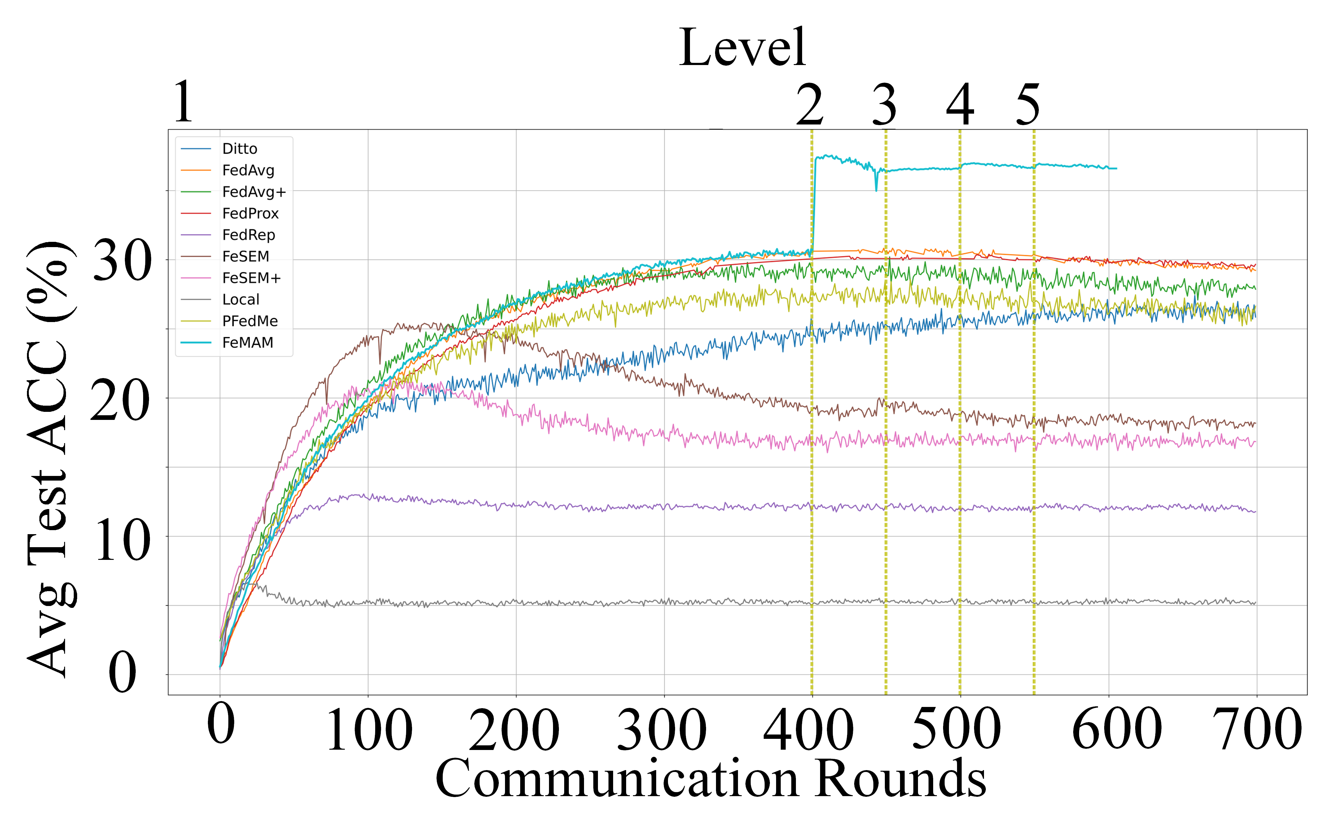
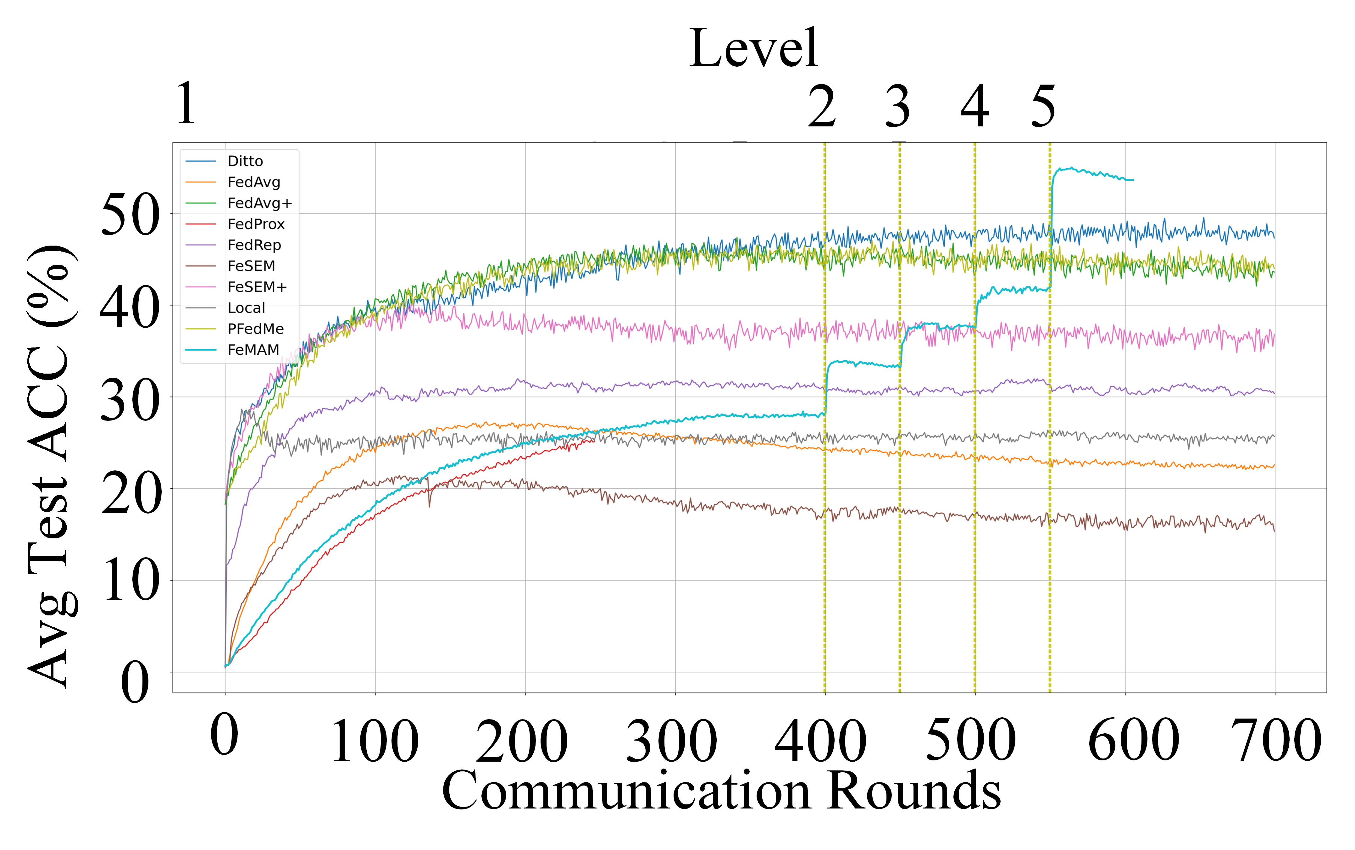
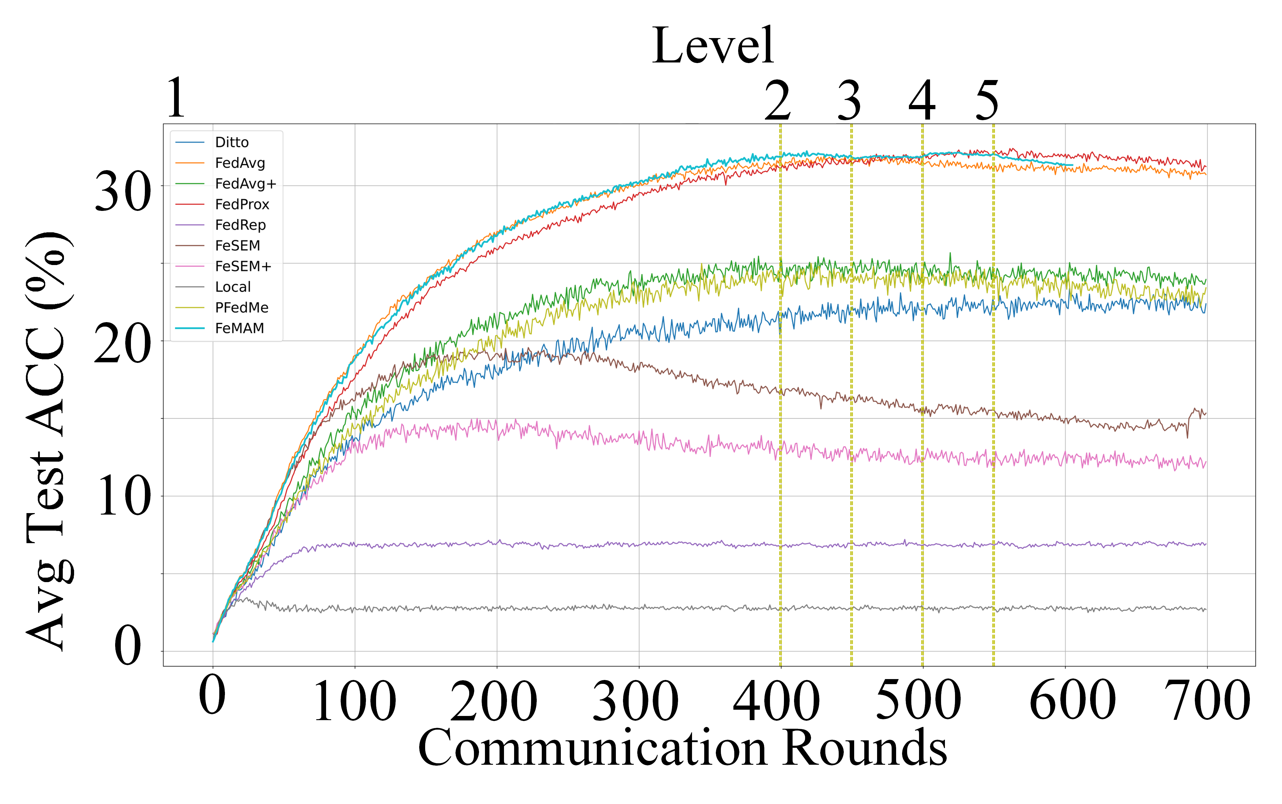
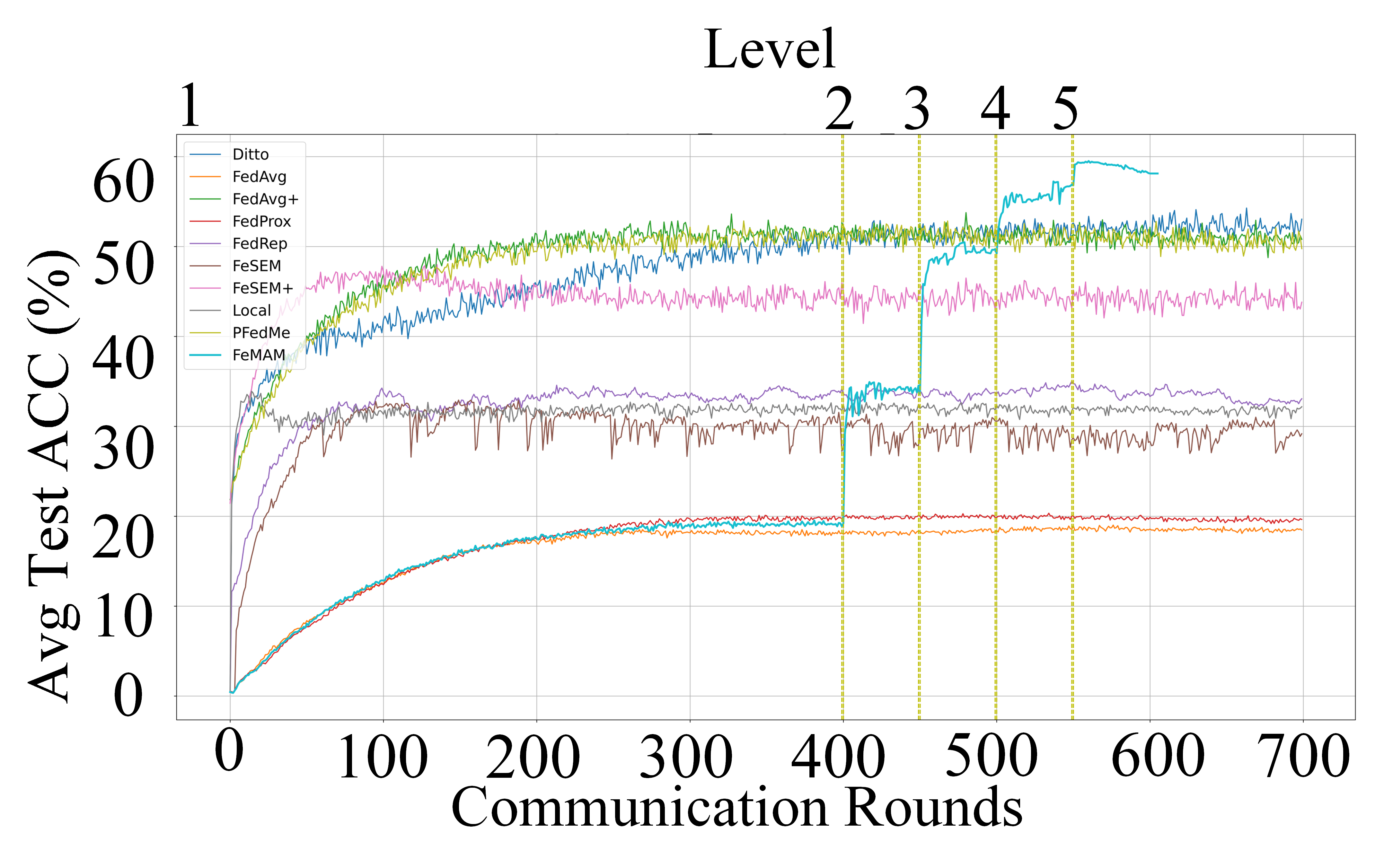
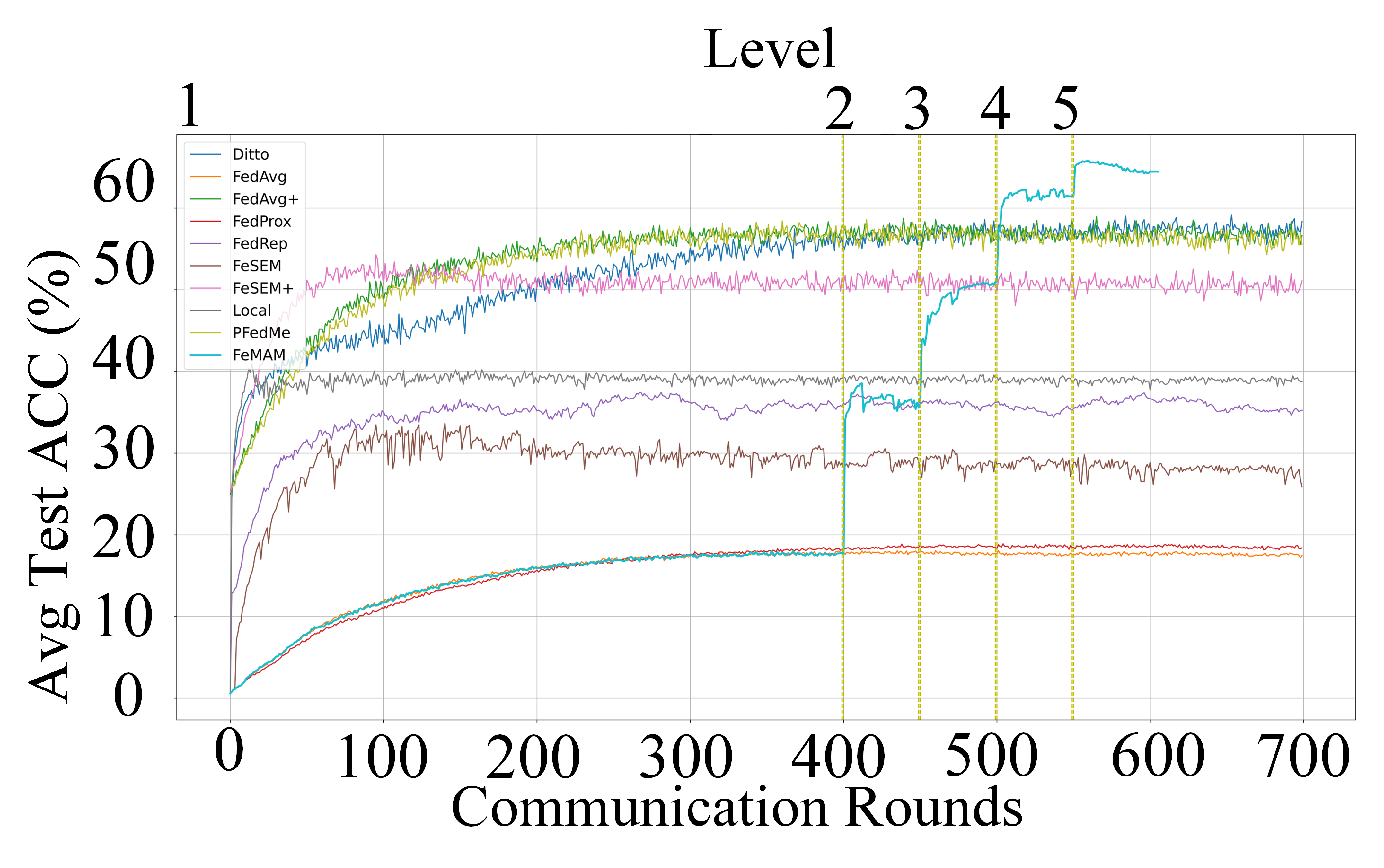
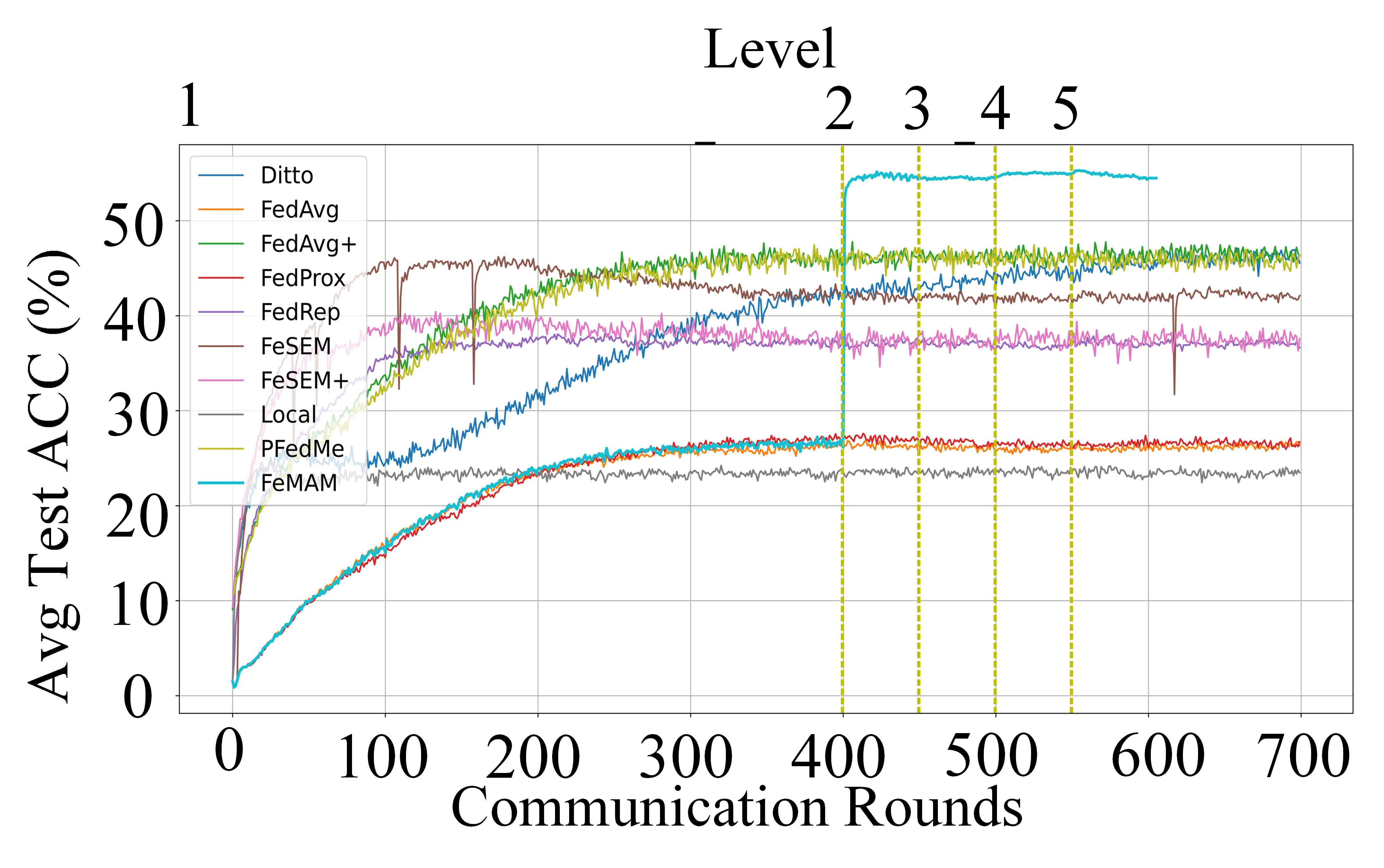
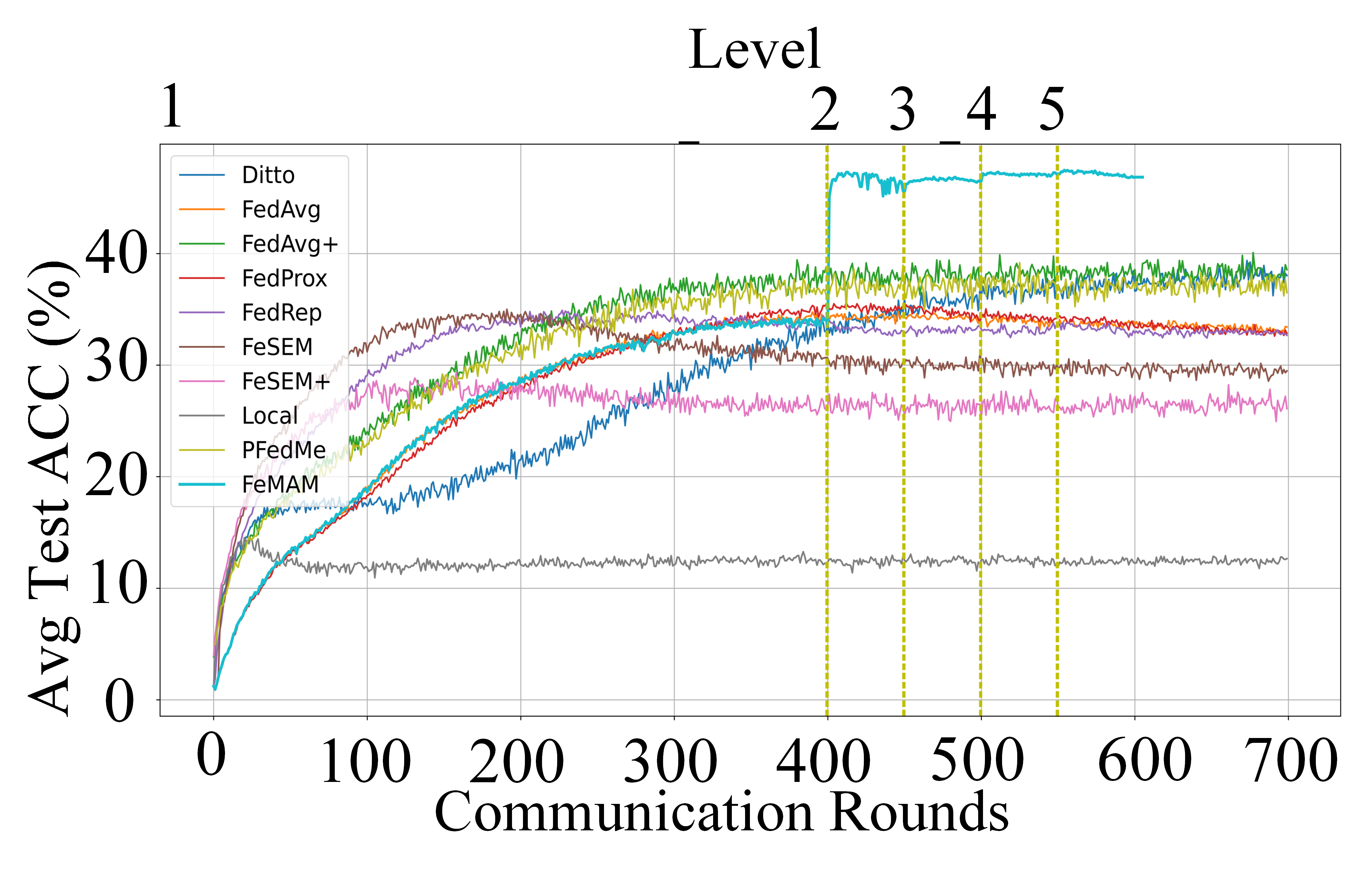
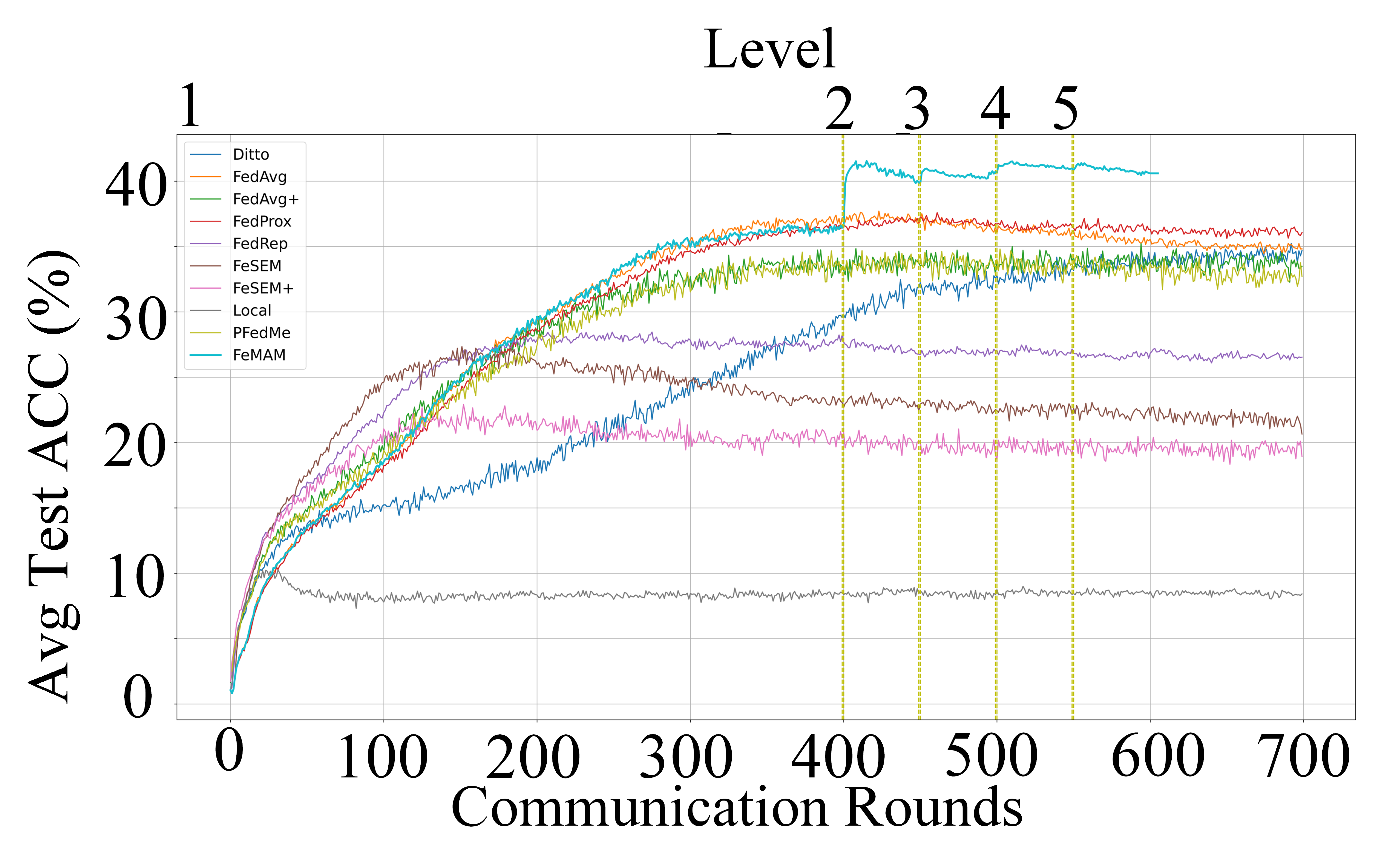
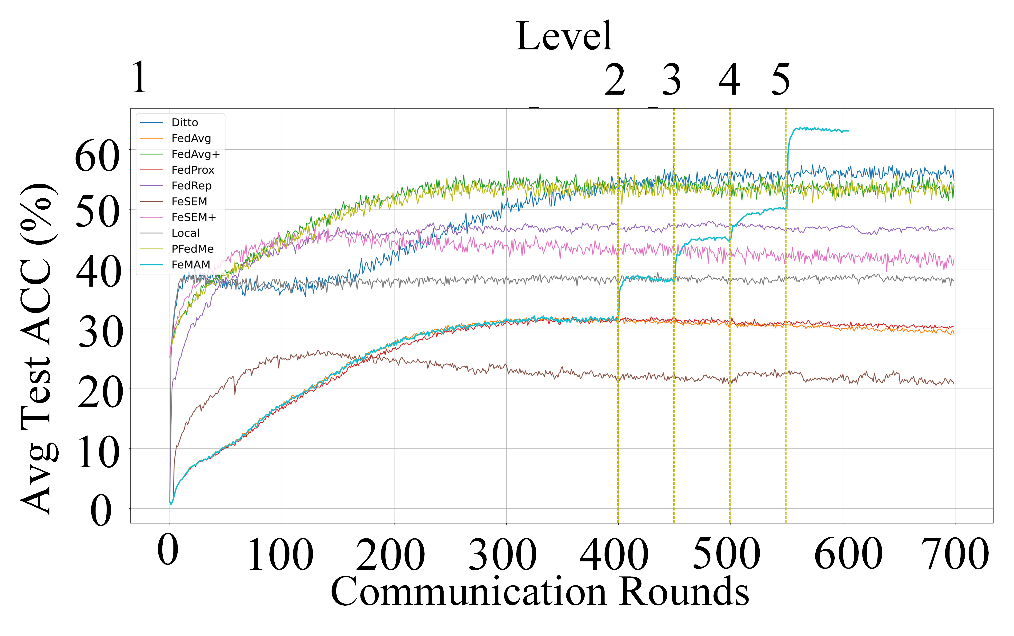
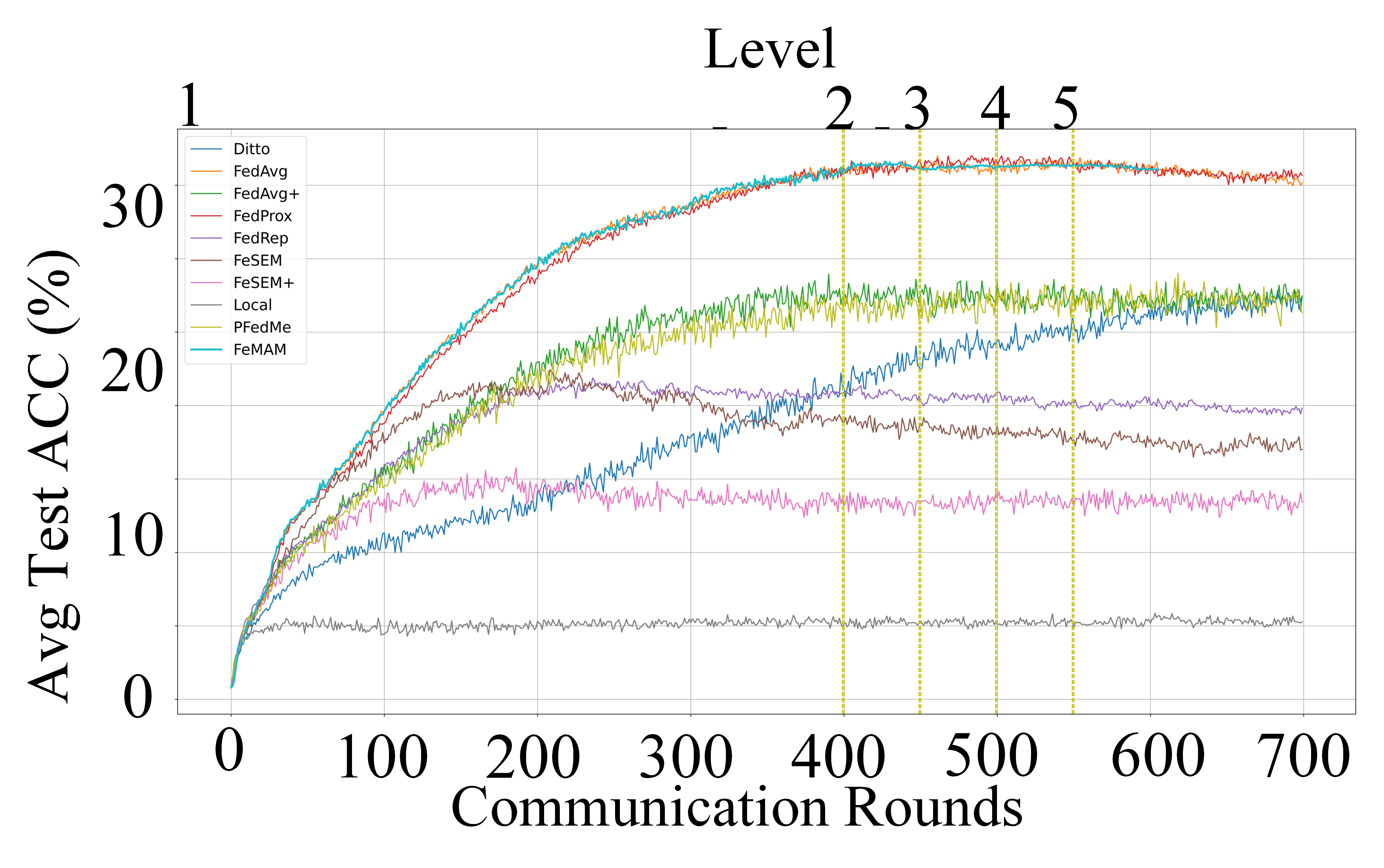
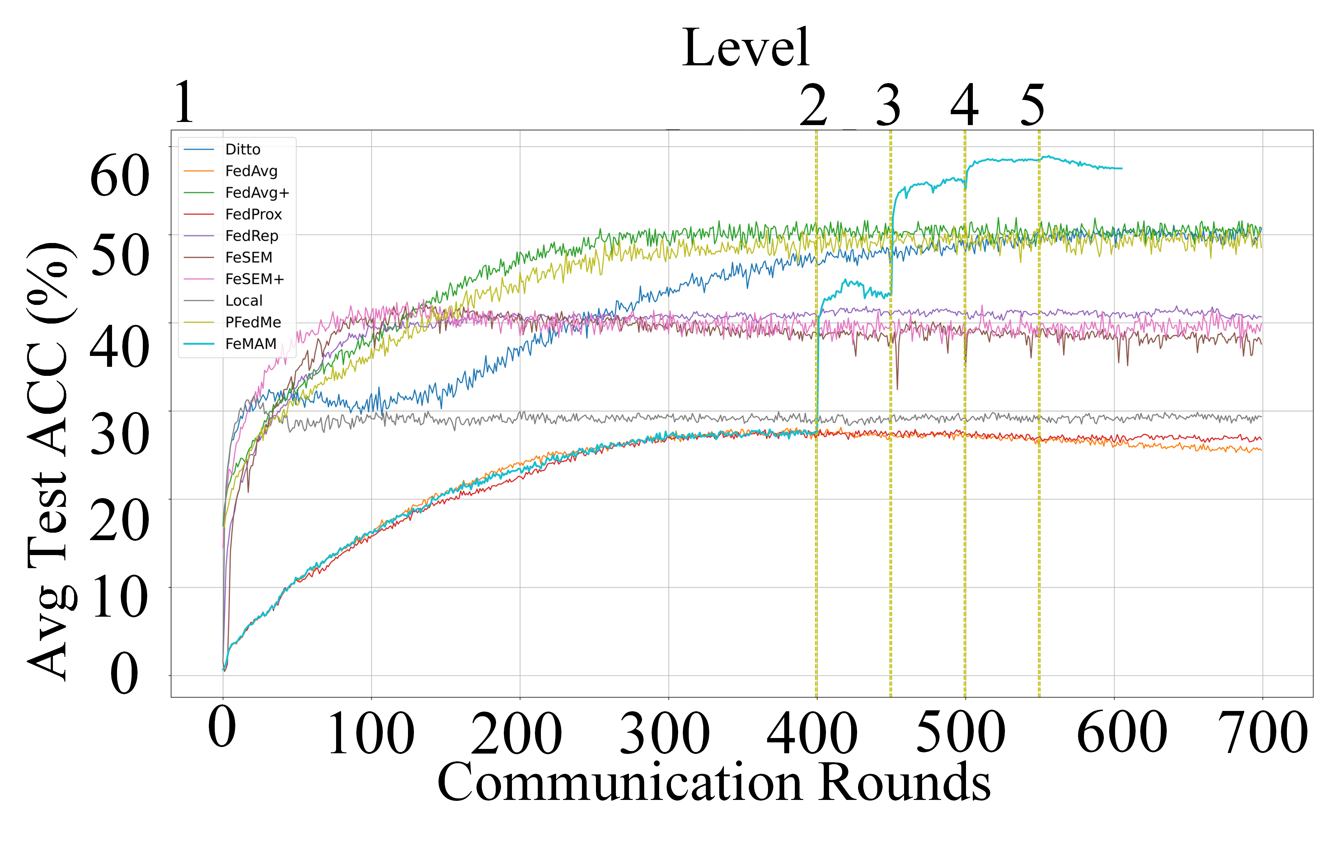
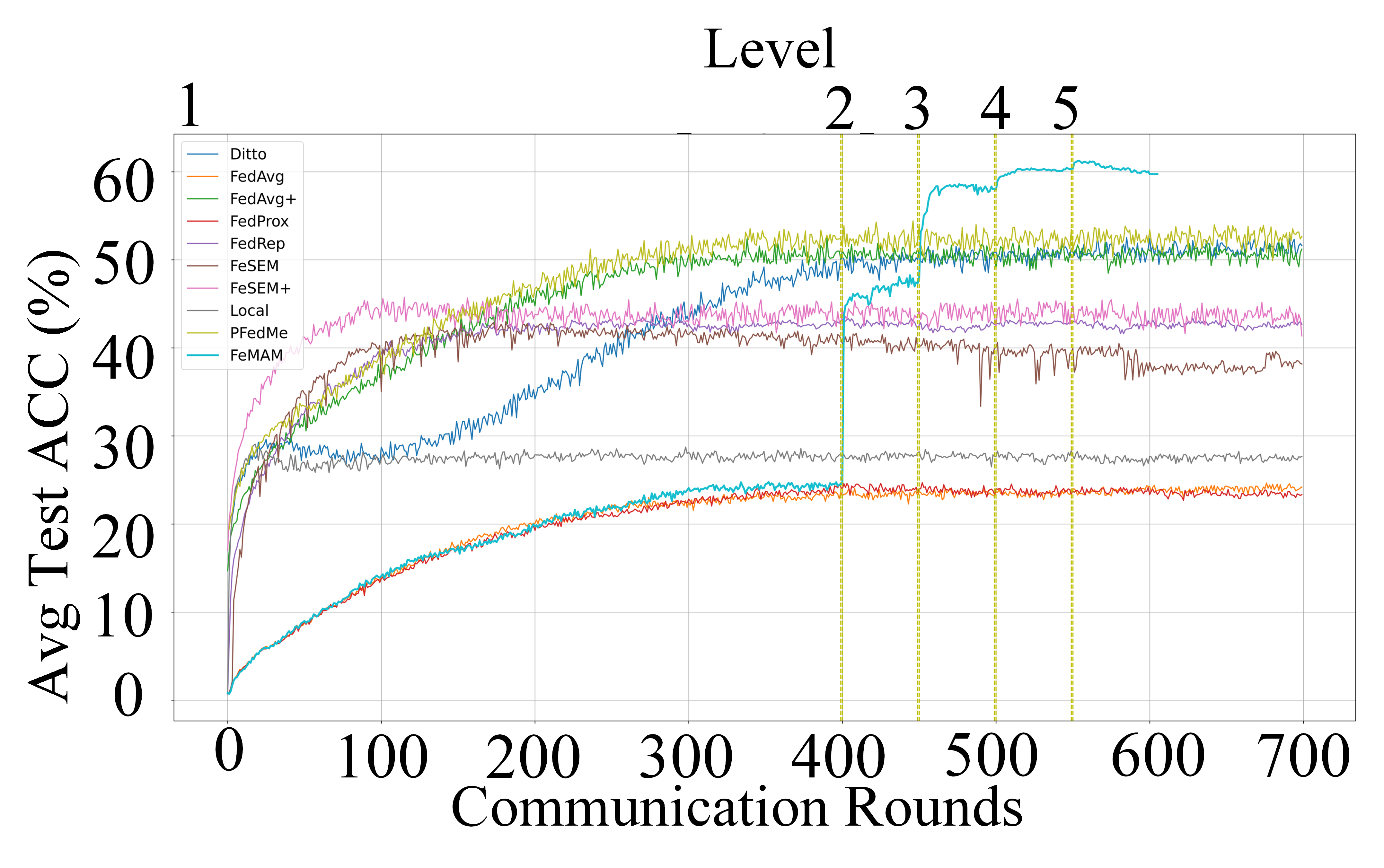
Fig. 3 compares the convergence of FeMAM and baselines with four types of non-IID.
Adaptive convergence across different types of non-IID: Levels are added progressively when the previous level converges, so the convergence curves are staircase-style. The more complex the data distribution is, the more levels of models are required, and the convergence curve have more plateaus. For example, IID in Fig. 3(d) only has one global level of structure, thus the convergence curve has one plateau; Client-wise in 3(b) and Multi-level in 3(c) is highly non-IID, so the inherent structure has plateaus on each of the the five levels; Cluster-wise in 3(a) has two levels, FeMAM use the first level to preserve globally shared knowledge and use the second level to capture the clustering structure.
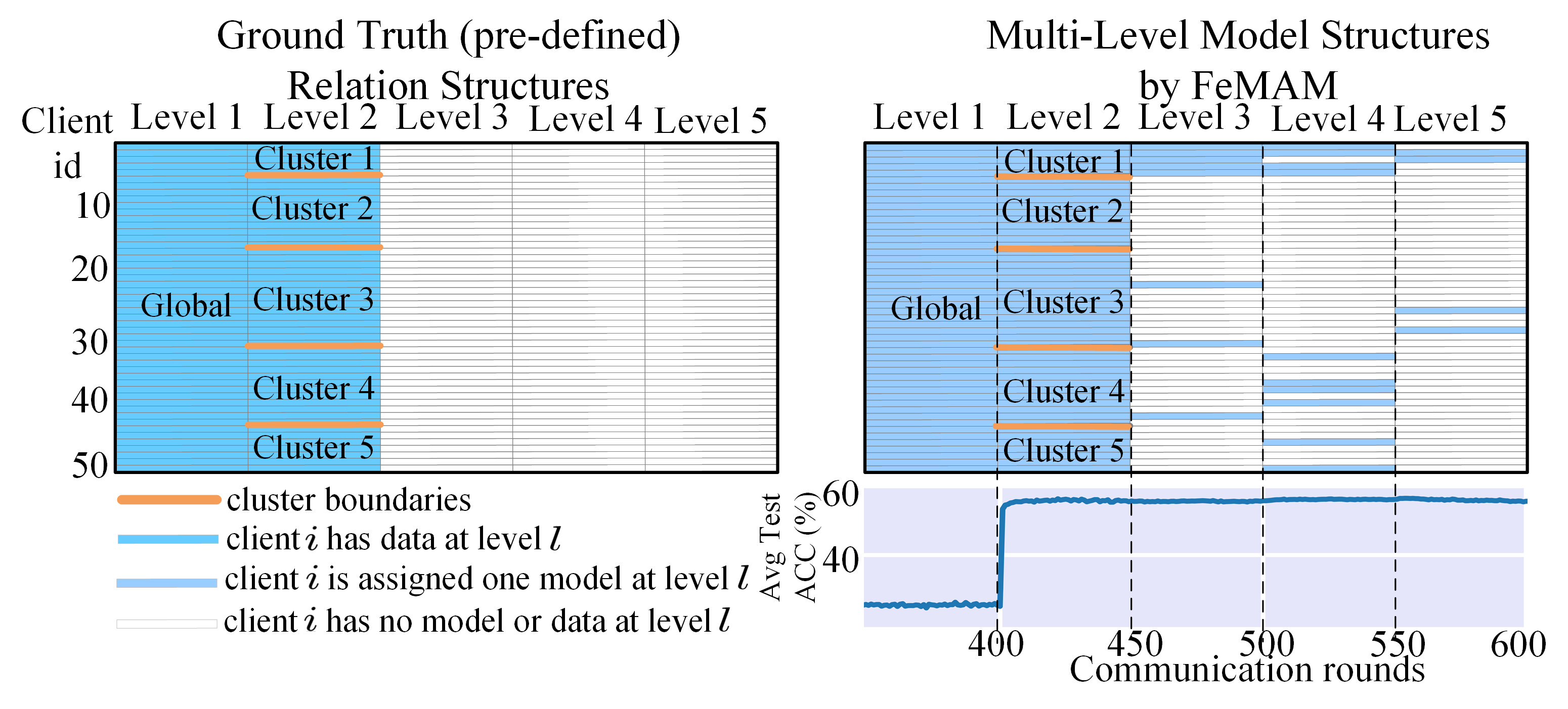
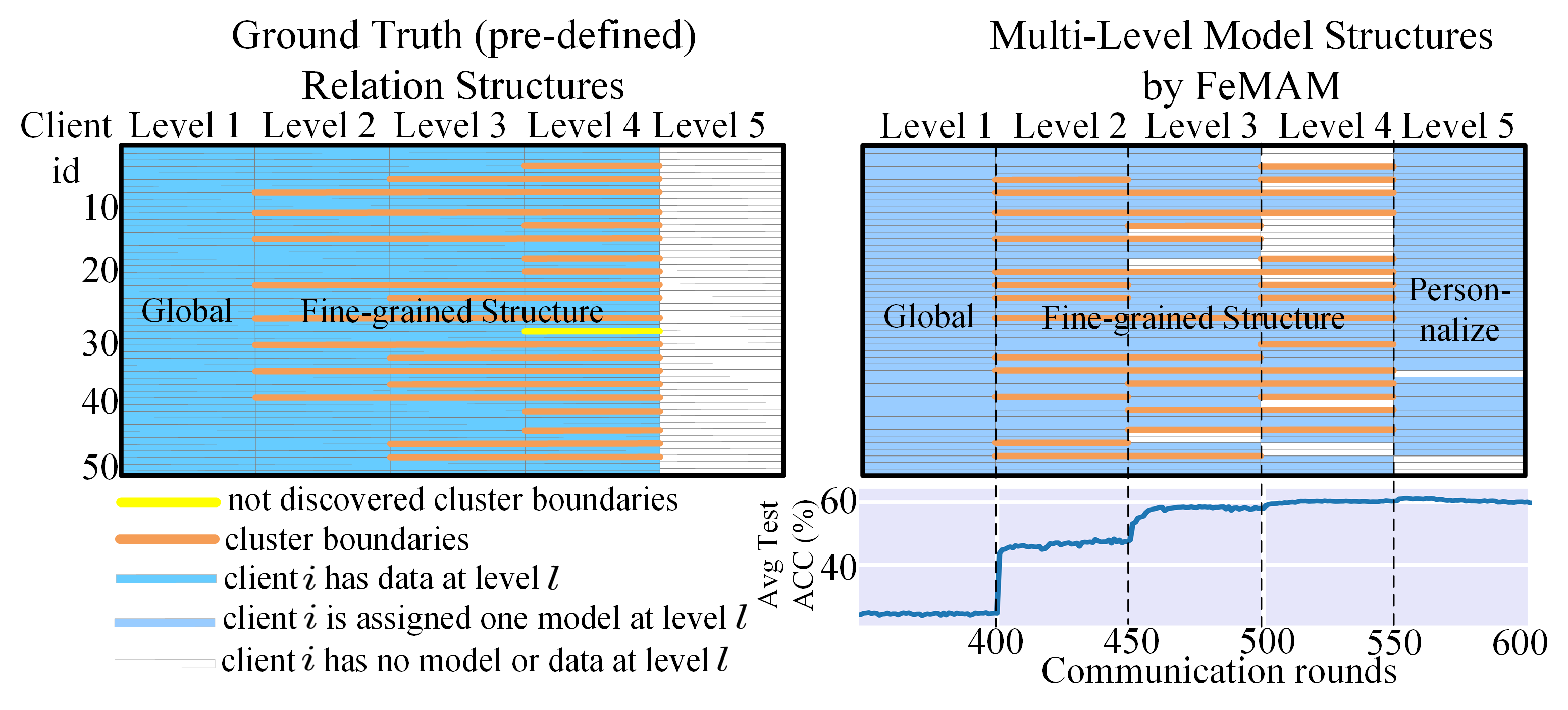
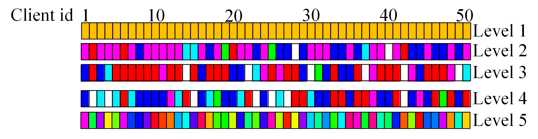
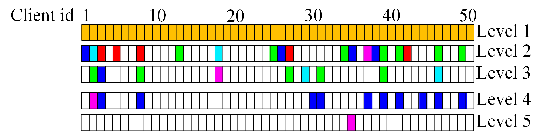
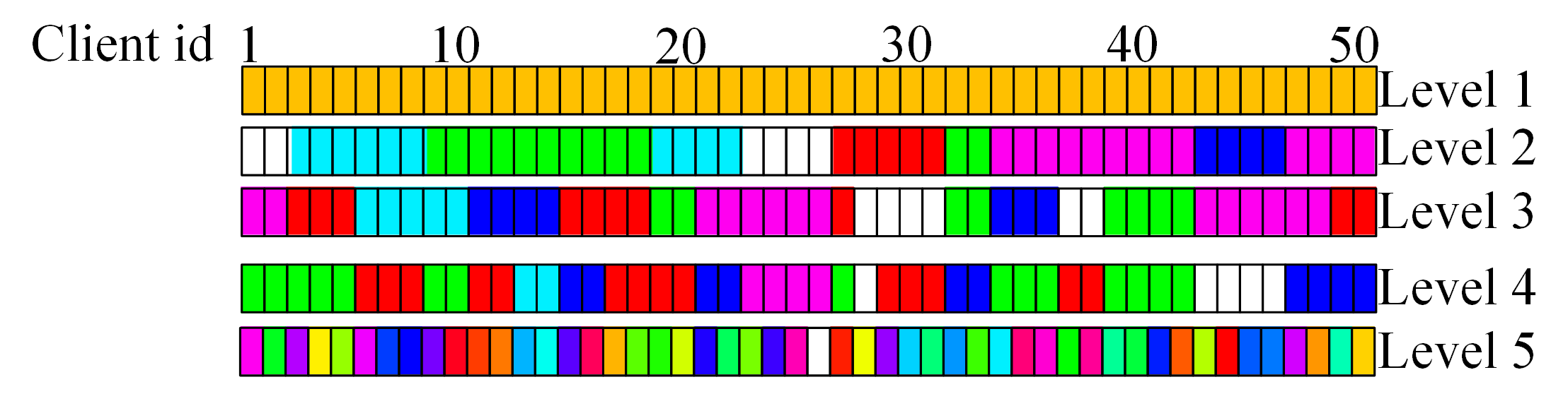
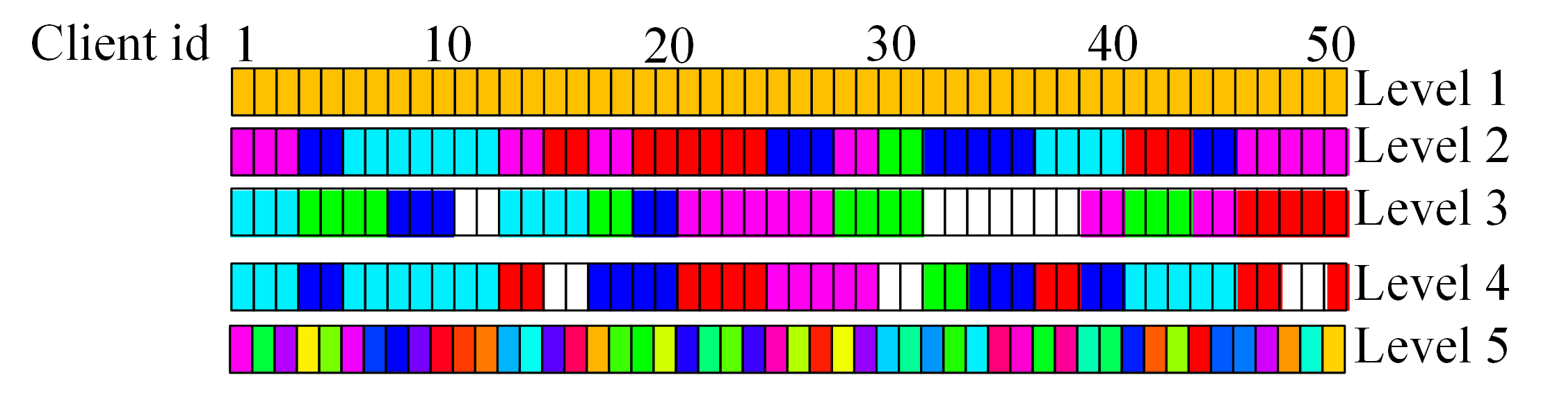
5.4 Analysis of Multi-level Structure
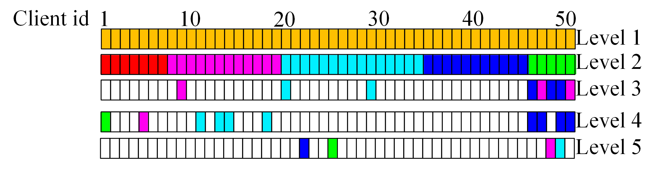
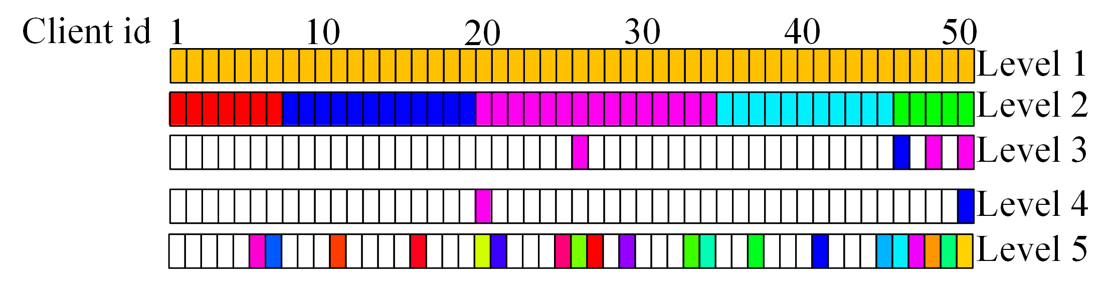
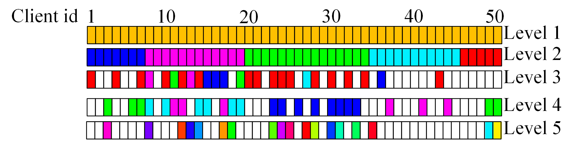
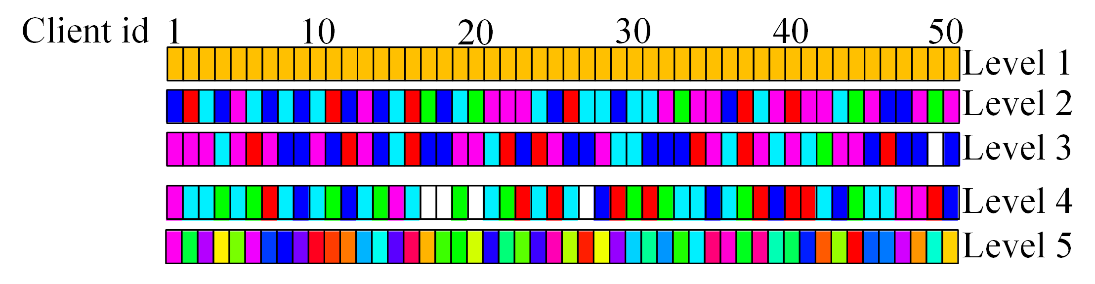
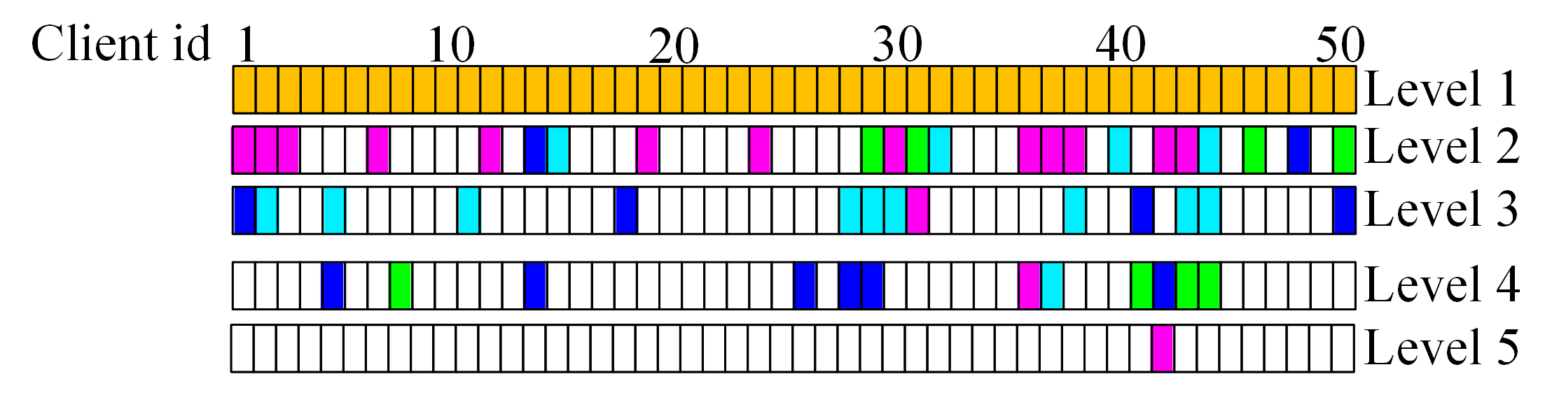
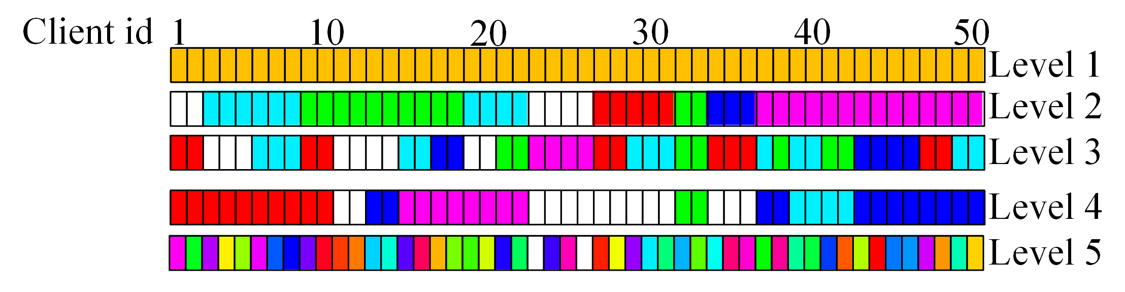
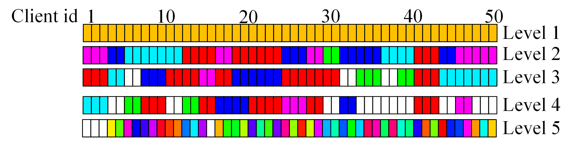
To understand how FeMAM discovers inherent data distribution, we visualize the multi-level structure generated by FeMAM through the mapping function in Fig. 4. We compare ground truth (pre-defined) relation structures on the right and place the convergence curves below for better understanding. Multi-level structure across all non-IID settings is in Appendix.
| Global | Cluster | Personalized | Accuracy | ||
| Level | 61.86 | ||||
| ✓ | ✓ | ✓ | ✓ | ✓ | |
| ✓ | ✓ | ✗ | ✗ | ✓ | |
| ✓ | ✗ | ✗ | ✗ | ✓ | |
| ✓ | ✓ | ✓ | ✓ | ✗ | |
| ✗ | ✓ | ✓ | ✓ | ✓ | |
FeMAM adapts to non-IID relation structures by pruning useless models: Under non-IID setting, for each client, the desired number of models varies. From Fig. 4, at level and , FeMAM preserves all the models, which corresponds to the dense levels and at the ground truth relation structure; From level to , FeMAM prunes most of the models, which corresponds to the empty levels from to at the ground truth relation structure.
FeMAM adapts to non-IID relation structures by discovering cluster boundaries: We mark the boundaries if the adjacent clients belong to different clusters. For ground truth relation structure in Fig. 4, the cluster knowledge is preserved in level marked by boundaries as five clusters; In multi-level model structures, by assigning each client with different clusters of models, FeMAM discovers all the boundaries at the corresponding level .
5.5 Ablation Study
Effects of Aggregation Methods To understand how different levels contribute to the final performance, we carry out an ablation study by varying the components of level-wise aggregation methods. We use multi-level setting since the data distribution structure is complex enough. As shown in Table 2, removing arbitrary levels will decrease performance, and the performance gain from different levels to a certain extent.
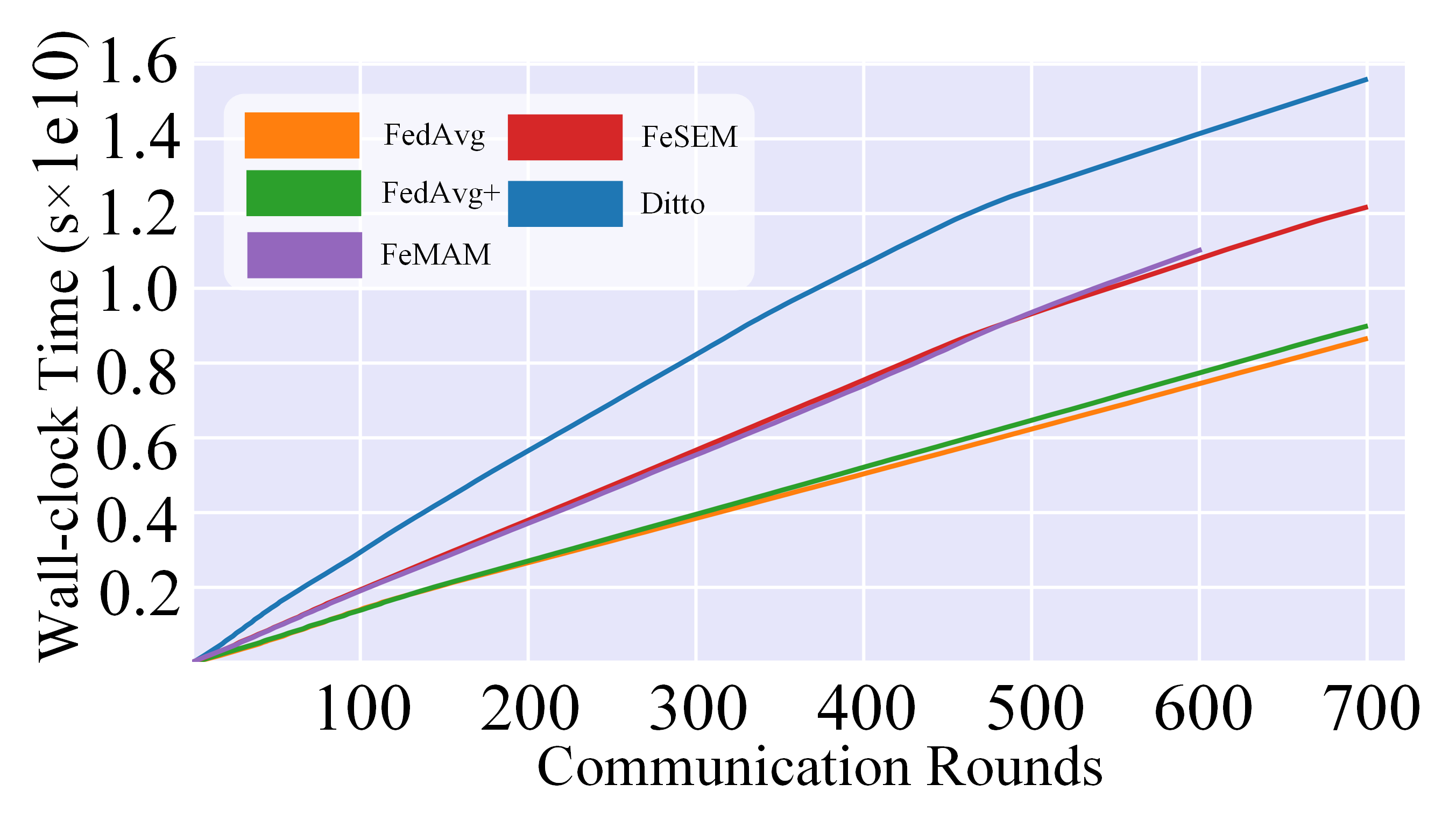
Running time. Fig. 5(a) shows the wall-clock time of FeMAM does not significantly exceed that of FedAvg and is less than Ditto, which makes it acceptable.
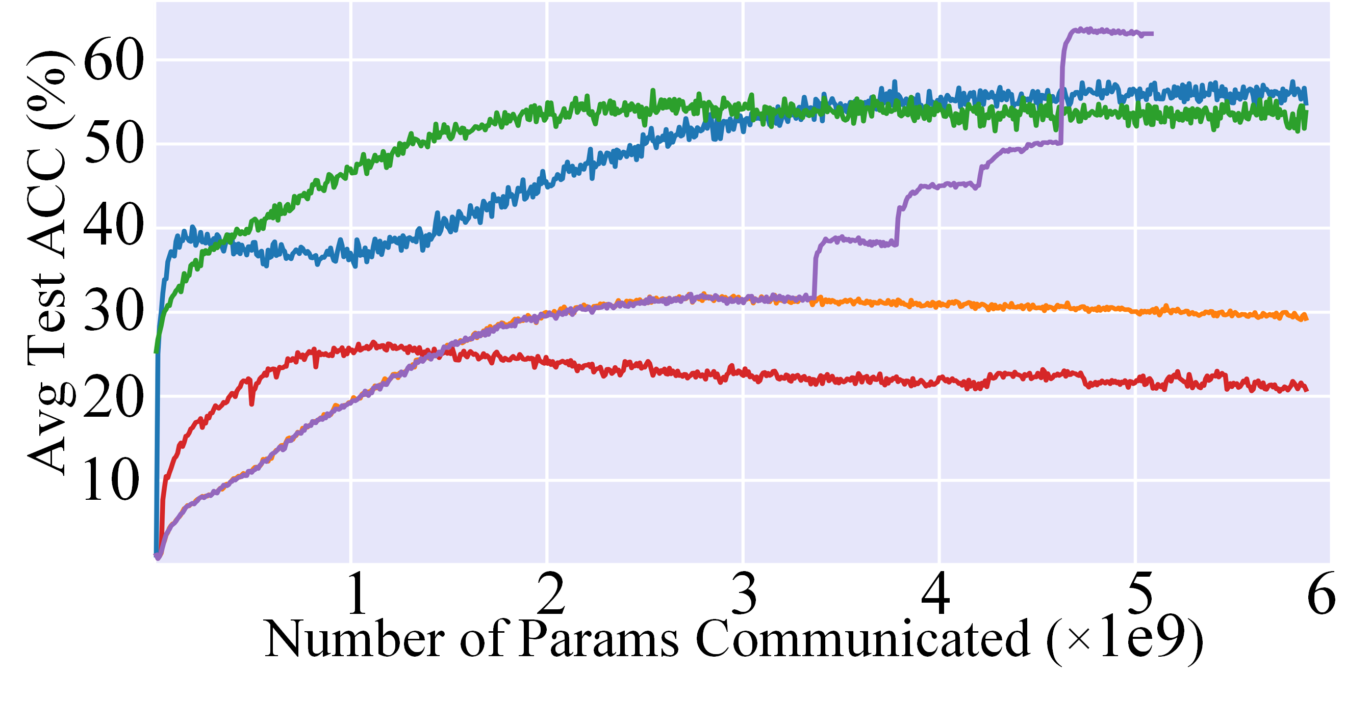
Communication Efficiency To understand the communication efficiency of FeMAM, we analyze how the test accuracy varies with the number of communicated parameters. For each client, FeMAM transmits one model per round, which is the same as other methods. As shown in Fig. 5(b), FeMAM achieves a high accuracy with acceptable communication-parameter volume.
6 Conclusion
In real FL applications, non-IIDness across clients is usually a complex hidden relation structure. This paper designs a structured FL framework that can learn the personalized models and relation structure simultaneously. In particular, the proposed multi-level structure is a straightforward architecture to approximate arbitrary hidden structures in real applications. Additive modeling is a key tool for linking many components to capture shared knowledge in a fine-grained manner. The proposed FeMAM demonstrates adaptability to a wide range of FL data distributions, from IID to non-IID, from distinctive structures to inherent structures. This is the first work on the multi-level non-IID problem in FL, and it is foreseen that many other solutions will be proposed in this direction.
References
- [1] Peter Kairouz, H Brendan McMahan, Brendan Avent, Aurélien Bellet, Mehdi Bennis, Arjun Nitin Bhagoji, Kallista Bonawitz, Zachary Charles, Graham Cormode, Rachel Cummings, et al. Advances and open problems in federated learning. Foundations and Trends® in Machine Learning, 14(1–2):1–210, 2021.
- [2] Jakub Konečnỳ, H Brendan McMahan, Felix X Yu, Peter Richtárik, Ananda Theertha Suresh, and Dave Bacon. Federated learning: Strategies for improving communication efficiency. arXiv preprint arXiv:1610.05492, 2016.
- [3] Tian Li, Anit Kumar Sahu, Ameet Talwalkar, and Virginia Smith. Federated learning: Challenges, methods, and future directions. IEEE signal processing magazine, 37(3):50–60, 2020.
- [4] Qiang Yang, Yang Liu, Tianjian Chen, and Yongxin Tong. Federated machine learning: Concept and applications. ACM Transactions on Intelligent Systems and Technology (TIST), 10(2):1–19, 2019.
- [5] Sixing Yu, J Pablo Muñoz, and Ali Jannesari. Federated foundation models: Privacy-preserving and collaborative learning for large models. arXiv preprint arXiv:2305.11414, 2023.
- [6] Zachary Charles, Nicole Mitchell, Krishna Pillutla, Michael Reneer, and Zachary Garrett. Towards federated foundation models: Scalable dataset pipelines for group-structured learning. Advances in Neural Information Processing Systems, 36, 2024.
- [7] Yue Zhao, Meng Li, Liangzhen Lai, Naveen Suda, Damon Civin, and Vikas Chandra. Federated learning with non-iid data. arXiv preprint arXiv:1806.00582, 2018.
- [8] Brendan McMahan, Eider Moore, Daniel Ramage, Seth Hampson, and Blaise Aguera y Arcas. Communication-efficient learning of deep networks from decentralized data. In Artificial intelligence and statistics, pages 1273–1282. PMLR, 2017.
- [9] Sai Praneeth Karimireddy, Satyen Kale, Mehryar Mohri, Sashank Reddi, Sebastian Stich, and Ananda Theertha Suresh. Scaffold: Stochastic controlled averaging for federated learning. In International Conference on Machine Learning, pages 5132–5143. PMLR, 2020.
- [10] Tian Li, Anit Kumar Sahu, Manzil Zaheer, Maziar Sanjabi, Ameet Talwalkar, and Virginia Smith. Federated optimization in heterogeneous networks. Proceedings of Machine Learning and Systems, 2:429–450, 2020.
- [11] Felix Sattler, Klaus-Robert Müller, and Wojciech Samek. Clustered federated learning: Model-agnostic distributed multitask optimization under privacy constraints. IEEE transactions on neural networks and learning systems, 32(8):3710–3722, 2020.
- [12] Avishek Ghosh, Jichan Chung, Dong Yin, and Kannan Ramchandran. An efficient framework for clustered federated learning. Advances in Neural Information Processing Systems, 33:19586–19597, 2020.
- [13] Ming Xie, Guodong Long, Tao Shen, Tianyi Zhou, Xianzhi Wang, Jing Jiang, and Chengqi Zhang. Multi-center federated learning. arXiv preprint arXiv:2108.08647, 2021.
- [14] Jie Ma, Ming Xie, and Guodong Long. Personalized federated learning with robust clustering against model poisoning. In Advanced Data Mining and Applications: 18th International Conference, ADMA 2022, Brisbane, QLD, Australia, November 28–30, 2022, Proceedings, Part II, pages 238–252. Springer, 2022.
- [15] Aviv Shamsian, Aviv Navon, Ethan Fetaya, and Gal Chechik. Personalized federated learning using hypernetworks. In International Conference on Machine Learning, pages 9489–9502. PMLR, 2021.
- [16] Tian Li, Shengyuan Hu, Ahmad Beirami, and Virginia Smith. Ditto: Fair and robust federated learning through personalization. In International Conference on Machine Learning, pages 6357–6368. PMLR, 2021.
- [17] Canh T Dinh, Nguyen Tran, and Josh Nguyen. Personalized federated learning with moreau envelopes. Advances in Neural Information Processing Systems, 33:21394–21405, 2020.
- [18] Alekh Agarwal, John Langford, and Chen-Yu Wei. Federated residual learning. arXiv preprint arXiv:2003.12880, 2020.
- [19] Xiaoxiao Li, Meirui Jiang, Xiaofei Zhang, Michael Kamp, and Qi Dou. Fedbn: Federated learning on non-iid features via local batch normalization. arXiv preprint arXiv:2102.07623, 2021.
- [20] Chunxu Zhang, Guodong Long, Tianyi Zhou, Peng Yan, Zijian Zhang, Chengqi Zhang, and Bo Yang. Dual personalization on federated recommendation. arXiv preprint arXiv:2301.08143, 2023.
- [21] Yue Tan, Yixin Liu, Guodong Long, Jing Jiang, Qinghua Lu, and Chengqi Zhang. Federated learning on non-iid graphs via structural knowledge sharing. In Proceedings of the AAAI conference on artificial intelligence, volume 37, pages 9953–9961, 2023.
- [22] Xiang Li, Kaixuan Huang, Wenhao Yang, Shusen Wang, and Zhihua Zhang. On the convergence of fedavg on non-iid data. arXiv preprint arXiv:1907.02189, 2019.
- [23] Christopher Briggs, Zhong Fan, and Peter Andras. Federated learning with hierarchical clustering of local updates to improve training on non-iid data. In 2020 International Joint Conference on Neural Networks (IJCNN), pages 1–9. IEEE, 2020.
- [24] Jie Ma, Guodong Long, Tianyi Zhou, Jing Jiang, and Chengqi Zhang. On the convergence of clustered federated learning. arXiv preprint arXiv:2202.06187, 2022.
- [25] Wenxuan Bao, Haohan Wang, Jun Wu, and Jingrui He. Optimizing the collaboration structure in cross-silo federated learning. arXiv preprint arXiv:2306.06508, 2023.
- [26] Alysa Ziying Tan, Han Yu, Lizhen Cui, and Qiang Yang. Toward personalized federated learning. IEEE Transactions on Neural Networks and Learning Systems, 2022.
- [27] Yue Wu, Shuaicheng Zhang, Wenchao Yu, Yanchi Liu, Quanquan Gu, Dawei Zhou, Haifeng Chen, and Wei Cheng. Personalized federated learning under mixture of distributions. arXiv preprint arXiv:2305.01068, 2023.
- [28] Jinheon Baek, Wonyong Jeong, Jiongdao Jin, Jaehong Yoon, and Sung Ju Hwang. Personalized subgraph federated learning. In International Conference on Machine Learning, pages 1396–1415. PMLR, 2023.
- [29] Jian Xu, Xinyi Tong, and Shao-Lun Huang. Personalized federated learning with feature alignment and classifier collaboration. arXiv preprint arXiv:2306.11867, 2023.
- [30] Yuhang Yao, Weizhao Jin, Srivatsan Ravi, and Carlee Joe-Wong. Fedgcn: Convergence and communication tradeoffs in federated training of graph convolutional networks. arXiv preprint arXiv:2201.12433, 2022.
- [31] Liangze Jiang and Tao Lin. Test-time robust personalization for federated learning. arXiv preprint arXiv:2205.10920, 2022.
- [32] Yue Tan, Guodong Long, Lu Liu, Tianyi Zhou, Qinghua Lu, Jing Jiang, and Chengqi Zhang. Fedproto: Federated prototype learning over heterogeneous devices. arXiv preprint arXiv:2105.00243, 2021.
- [33] Liam Collins, Hamed Hassani, Aryan Mokhtari, and Sanjay Shakkottai. Exploiting shared representations for personalized federated learning. In International Conference on Machine Learning, pages 2089–2099. PMLR, 2021.
- [34] Jie Ma, Tianyi Zhou, Guodong Long, Jing Jiang, and Chengqi Zhang. Structured federated learning through clustered additive modeling. Advances in Neural Information Processing Systems, 36, 2023.
- [35] Zhiwei Li, Guodong Long, and Tianyi Zhou. Federated recommendation with additive personalization. arXiv preprint arXiv:2301.09109, 2023.
- [36] Ya Le and Xuan S. Yang. Tiny imagenet visual recognition challenge. 2015.
- [37] Alex Krizhevsky, Geoffrey Hinton, et al. Learning multiple layers of features from tiny images. 2009.
- [38] Kaiming He, Xiangyu Zhang, Shaoqing Ren, and Jian Sun. Deep residual learning for image recognition. In Proceedings of the IEEE conference on computer vision and pattern recognition, pages 770–778, 2016.
- [39] Tzu-Ming Harry Hsu, Hang Qi, and Matthew Brown. Measuring the effects of non-identical data distribution for federated visual classification. arXiv preprint arXiv:1909.06335, 2019.
Appendix
Appendix A No Free Lunch
No such thing as a free lunch. Our proposed method can improve accuracy by learning the multi-level non-IID across clients. However, the cost is increasing the load of computation and communication in the training phase. In terms of communication efficiency, our proposed FeMAM takes level-wise alternating optimization that the client only needs to download and update the model at the latest level. Therefore, the communication cost per round is equivalent to the specific level-wise FL methods, i.e., FedAvg and FeSEM. As shown in Fig. 5(b), FeMAM is communication efficient and achieves a high accuracy with acceptable communicate-parameter volume. Another factor that needs to be considered is the convergence rate. As demonstrated in Fig. 3, the five-level FeMAM is equivalent to FedAvg when it is training on level one. When the FeMAM starts to train on levels 2-5, it could converge very quickly in 50 communication rounds. Also, it is worth noting that the model training-related computation cost and runtime will also be impacted accordingly by the increasing communication rounds. In practice, as shown in the experiments, Fig. 5(a), the communication rate of FeMAM is less than FedAvg and greater than Ditto, which is acceptable comparing to the accuracy improvement in Table 1.
The FeMAM needs to store up to global models for model inferences. It will incur special storage costs and model inference costs. In general, the value of is usually set to be five to cover most of existing non-IID in FL. As in Fig. A.1, some clients select a subset of levels, and not every client will store all levels. First, in the cluster-wise non-IID, most clients in FeMAM only use two or three levels which is similar to many clustered FL methods. Second, for IID scenarios, most clients in FeMAM will use only one model from level one which is equivalent to FedAvg. Third, for client-wise and multi-level non-IID, the clients of FeMAM will use more global models at different levels to fully capture the multi-level non-IID, and the storage and model inference-related computation cost will be increased to times. The model inference-related computation cost is relatively small and the increased cost is still acceptable for most smart devices.
Appendix B Level-wise Optimization and Complete Algorithm
Given the multi-level structure, the level-wise alternating minimization schema is proposed to efficiently solve the proposed objective function in Eq. (5). Specifically, each level of global models is iteratively optimized while fixing other levels. Algorithm 2 gives out the complete optimizing procedure of FeMAM.
We define the general aggregation and broadcast operation at level as below:
| (B.1a) | ||||
| (B.1b) | ||||
where is the set of local clients that assigned to. is thus the inverse mapping function of , e.g., . We will illustrate the level-wise update scheme below.
(i) Update One Globally Shared Model For the globally shared model at level , we optimize the global model . The optimization can be addressed by two iterative steps. First, each client conduct a local learning-based gradient descent step with learning rate below:
| (B.2) |
Second, the global model is updated by aggregating client’s updated local models using Eq. (B.1b), and also by setting .
(ii) Update Clustered Shared Models For the clustered shared models from Level 2 to , we optimize the level-’s models with all the other level’s models fixed. The solving steps to the problem in Eq. (5) reduces to a clustered FL problem. Specifically, we adopt K-means to embody the clustering algorithm. The clustering assignments are updated as follows:
| (B.3) |
and then the cluster centroids are updated using the general form of Eq. (B.1b).
At local learning, we optimize with fixed. The optimization is addressed by gradient descent step with learning rate :
| (B.4) |
(iii) Update Personalized Model on Clients For the last level , we optimize each model at the -th level with other levels fixed. A gradient descent step is conducted as local optimization:
| (B.5) |
The model is for preserving personalized knowledge, thus it is not necessary to be aggregated.
Appendix C Experiments
C.1 Hyper-parameter Settings
FL system settings The number of clients is set to be . The local training epochs is set to be . Learning rate is . We use resnet- as basic models. The total number of training epochs is set to be 700. We use validate dataset to monitor the performance and select the checkpoint with the minimum evaluation error. The validate dataset is split from the original training set in Tiny ImageNet and CIFAR-100, and is set to have the half number of samples as the test set. Thus, for CIFAR-100, the number of training set, validation set and test set is 45000, 5000 and 10000 respectively. Also, for Tiny ImageNet, the number of training set, validation set and test set is 95000, 5000 and 10000 respectively.
Data partition Settings For the cluster-wise partition, each cluster is evenly assigned to a fixed number of class. For instance, means there are five clusters and each cluster is assigned to class. Each cluster is then evenly divided and assign to some clients. For the multi-level partition, we basically follow the same rule as cluster-wise partition at each level, except that we first split the dataset into parts by class, where is the number of levels. Then each level is divided in a cluster-wise manner. Based on the intuition of multi-level structure in real world, we further assume that levels with smaller clusters have larger number of samples, which means that more basic concepts are more commonly shared. For example, means the first level has clusters, the second level has clusters, and the third level has clusters. Note that the last level of Tiny ImagNet has more than 20 clusters, which means that it is highly personalized. We give out the ground truth multi-level assignments for each settings in Table C.1. Finally, the client-wise setting uses the Dirichlet distribution to control the randomness of non-IID data. This is a standard method used in most personalized FL methods, which are usually client-wise non-IID.
| data- set |
level
id |
class
num |
cluster
num |
data distribution structure |
| CIFAR-100 | 1 | 19 | 2 |
![[Uncaptioned image]](/html/2405.16472/assets/figure/gdcifar259.png)
|
| 2 | 7 | 5 | ||
| 3 | 3 | 9 | ||
| 1 | 14 | 3 |
![[Uncaptioned image]](/html/2405.16472/assets/figure/gdcifar3611.png)
|
|
| 2 | 6 | 6 | ||
| 3 | 2 | 11 | ||
| Tiny ImageNet | 1 | 20 | 4 |
![[Uncaptioned image]](/html/2405.16472/assets/figure/gdtiny471.png)
|
| 2 | 6 | 13 | ||
| 3 | 2 | 21 | ||
| 1 | 9 | 9 |
![[Uncaptioned image]](/html/2405.16472/assets/figure/gdtiny667.png)
|
|
| 2 | 5 | 15 | ||
| 3 | 2 | 22 |
Local Each client train with its own training and validation dataset.
FedAvg and FedAvg+ The global model’s performance and the performance of each local model by FedAvg algorithm, respectively.
FedProx The coefficient is set to be .
PFedMe , .
FedRep The local training rounds for body and head are both set to be .
Ditto The coefficient is set to be .
FeSEM and FeSEM+ The global model’s performance and the performance of each local model by FeSEM algorithm, respectively. The number of clusters is set to be .
FeMAM We do not finetune hyper-parameters for each data distribution setting, and all the hyper-parameters mentioned below are fixed to be the same for all non-IID settings across all datasets. The number of levels is set to be . To ensure the convergence of FedAvg, the training epochs for the first level is set to be . At every communication rounds, only the last level of models are trained and the previous level of models are fixed and act as and add on to the final prediction. The first level is FedAvg, the second to fourth level is set to be FeSEM with clusters, and finally the fifth level is set as local training. For each level, we first train until converge. Then for each client, we check if the new model has reduced the validation error. We only add models that reduce the validation error to the existing structure. To monitor the convergence, we check the variance of the overall accuracy in the latest communication rounds. If it is smaller than , then FeMAM is converged at the current level. During experiments we found that with FeAvg as the first level, all the subsequent levels converged quickly in epochs.
C.2 Further Analysis of Multi-level Structure
To understand how FeMAM discovers inherent data distribution, we visualize the multi-level structure generated by FeMAM through the mapping function in Fig. A.1. We compare ground truth (pre-defined) relation structures on the right and place the convergence curves below for better understanding. We use the Tiny ImageNet dataset to illustrate the observations and the results on CIFRA-100 are similar.
FeMAM adapts to different non-IID relation structures by pruning useless models: Generally, for each non-IID setting, the desired number of models per level varies. From Fig. 1(a) and Fig.1(d), the ground truth relation structures are empty at high levels, so FeMAM generate relatively sparse structures on Cluster-wise and IID data. In Fig.1(b) and Fig.1(c), FeMAM needs more levels to capture the relatively complex relation structure of client-wise and multi-level non-IID data.
FeMAM adapts to different non-IID relation structures by discover cluster boundaries: For each level, we mark the boundaries if the adjacent clients belong to different clusters. Thus, the cluster boundaries on the ground truth relation structure represents the data distribution. Note that Client-wise and IID setting do not have explicit clusters, so we do not mark boundaries in Fig.1(b) and Fig.1(d). For simple cluster structure in Fig.1(a), FeMAM discovers all the boundaries at the corresponding level ; For complex, multi-level structure in Fig.1(c), FeMAM reveals almost all the boundaries except one, but at different levels. Note that the number of clusters of FeMAM from level 2 to 4 is simply set to 5, so we do not expect FeMAM to completely reveal the multi-level ground truth clusters at each level, which is 9, 15 and 22 respectively.
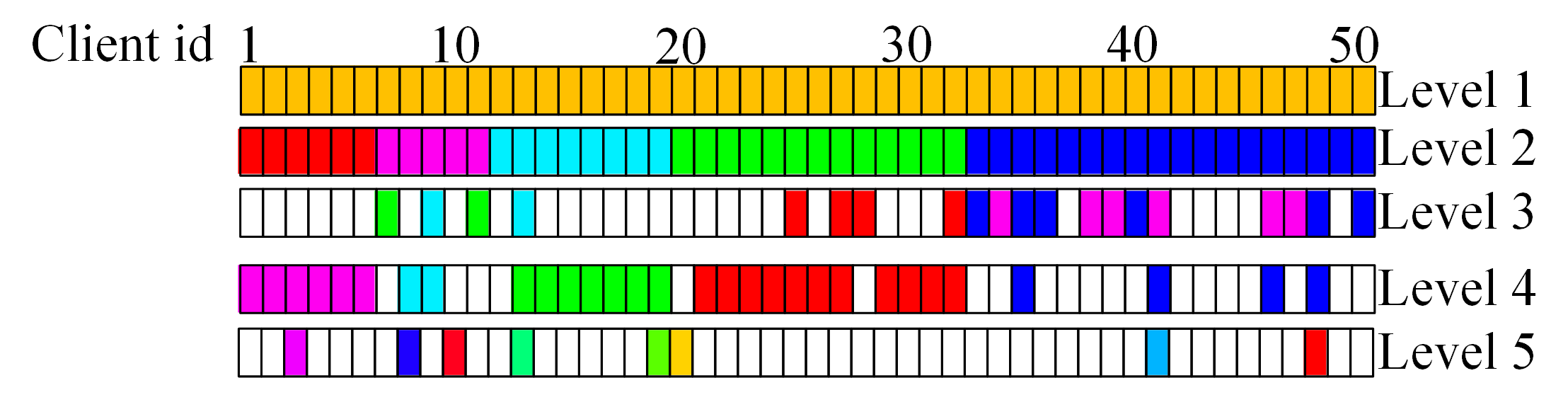
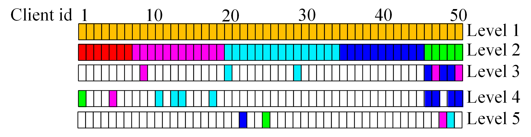
C.3 Visualization of Multi-level Model Structures for Tiny ImageNet and CIFAR-100 on Every Data Partitions
To explicitly show all the multi-level model structures, We use different colors to distinguish between different models in the cells in Fig. A.1. We visualize all the Multi-level Model Structures in Fig. C.2 and Fig. C.4, produced by FeMAM on CIFAR-100 and Tiny ImageNet dataset with three data partition settings, i.e., cluster-wise, client-wise and multi-level. Note that the Cluster-wise, , Client-wise, , Multi-level,, and IID in Fig. C.4 is the same Multi-level Model Structure as in Fig. A.1, expect that we rotated the image degrees clockwise and used different colors to distinguish between different models in the cells.

C.4 Numerical results for Tiny ImageNet and CIFAR-100 on Every Data Partitions
C.5 Analyzing Underperformance on Dataset
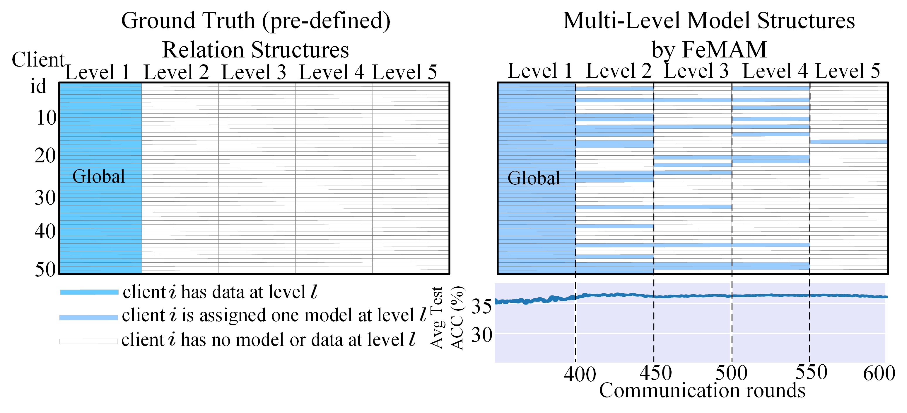
For IID, from Table C.3, FedProx achieves the highest Accuracy and Macro-F1 score. Also, The scores of FedAvg, FedProx and FeMAM are very close. From the convergence curves in Fig. C.6 and Fig. C.8, the behavior of FedProx, FedAvg and FeMAM are almost the same, and are above other methods.In fact, according to the FeMAM structure for IID data in Fig. C.2 and Fig. C.4, only a few models appear at levels other than the first,, which means FeMAM is almost equivalent to FedAvg. This indicates that under the IID setting, FedAvg-like methods are the optimal choice, and the performance is hard to improve by adding more models.
| Datasets | TinyImagenet | CIFAR-100 | ||||||||||
|---|---|---|---|---|---|---|---|---|---|---|---|---|
| Clusters | ||||||||||||
| Methods | Accuracy | Macro-F1 | Accuracy | Macro-F1 | Accuracy | Macro-F1 | Accuracy | Macro-F1 | Accuracy | Macro-F1 | Accuracy | Macro-F1 |
| Local | 15.570.03 | 10.420.17 | 10.160.31 | 5.670.12 | 6.370.15 | 2.850.06 | 22.810.11 | 13.800.33 | 13.820.15 | 7.200.05 | 9.800.29 | 4.720.06 |
| FedAvg | 24.870.80 | 12.630.49 | 28.080.24 | 18.330.30 | 26.440.40 | 14.550.39 | 29.280.48 | 12.730.15 | 34.040.35 | 23.320.34 | 36.490.07 | 28.770.05 |
| FedAvg+ | 36.740.09 | 32.970.23 | 32.520.18 | 27.130.24 | 28.760.48 | 22.650.22 | 46.670.74 | 39.770.91 | 37.730.62 | 31.860.95 | 33.600.40 | 27.350.57 |
| FedProx | 23.831.56 | 12.160.64 | 26.361.80 | 17.071.28 | 30.280.15 | 22.160.14 | 27.520.44 | 15.610.25 | 34.250.26 | 23.680.32 | 36.570.31 | 28.710.36 |
| PFedMe | 38.760.31 | 34.870.45 | 32.120.06 | 26.970.07 | 27.460.35 | 21.420.29 | 46.300.31 | 39.050.36 | 36.720.69 | 30.580.87 | 33.320.42 | 27.160.48 |
| FedRep | 20.490.49 | 16.570.34 | 15.640.54 | 11.270.58 | 10.380.93 | 6.490.06 | 36.750.41 | 29.990.30 | 33.580.53 | 28.140.79 | 27.670.17 | 22.550.18 |
| Ditto | 37.120.70 | 33.740.80 | 31.100.84 | 26.260.78 | 24.690.04 | 19.150.01 | 45.160.18 | 38.050.76 | 36.580.41 | 31.090.42 | 32.480.67 | 27.510.59 |
| FeSEM | 41.200.25 | 37.820.21 | 32.680.26 | 27.450.10 | 25.550.62 | 20.130.82 | 45.100.51 | 38.730.60 | 34.090.10 | 29.060.15 | 26.560.21 | 21.570.12 |
| FeSEM+ | 31.600.42 | 26.720.61 | 25.780.62 | 19.820.73 | 19.510.26 | 13.770.17 | 37.330.99 | 29.701.41 | 27.310.32 | 21.200.14 | 21.380.48 | 15.940.75 |
| FeMAM | 46.800.35 | 43.290.34 | 39.930.11 | 34.330.12 | 35.820.29 | 29.500.29 | 53.720.29 | 48.330.40 | 46.080.21 | 41.880.30 | 40.360.12 | 36.050.04 |
| Datasets | TinyImagenet | CIFAR-100 | ||||||
|---|---|---|---|---|---|---|---|---|
| IID / | IID | 0.1 | IID | 0.1 | ||||
| Methods | Accuracy | Macro-F1 | Accuracy | Macro-F1 | Accuracy | Macro-F1 | Accuracy | Macro-F1 |
| Local | 2.950.01 | 1.280.03 | 28.930.21 | 8.000.15 | 5.070.09 | 2.210.07 | 38.570.15 | 11.900.11 |
| FedAvg | 32.200.36 | 22.810.32 | 24.330.34 | 8.730.24 | 36.630.27 | 29.850.33 | 30.460.15 | 11.530.08 |
| FedAvg+ | 24.120.02 | 17.170.08 | 45.850.13 | 23.840.03 | 27.420.58 | 21.530.55 | 53.570.45 | 29.490.41 |
| FedProx | 32.490.14 | 23.060.13 | 23.320.36 | 8.600.33 | 36.780.19 | 30.020.19 | 30.850.45 | 11.680.23 |
| PFedMe | 24.070.26 | 16.840.33 | 44.730.54 | 22.570.79 | 26.970.57 | 21.120.60 | 53.740.09 | 28.680.20 |
| FedRep | 4.640.22 | 2.510.15 | 27.990.03 | 10.190.31 | 20.310.18 | 15.350.15 | 46.650.48 | 22.220.45 |
| Ditto | 22.170.31 | 14.950.36 | 47.080.16 | 24.570.23 | 27.050.83 | 21.610.68 | 56.060.48 | 30.710.34 |
| FeSEM | 18.870.53 | 12.600.44 | 22.340.79 | 7.790.19 | 20.820.93 | 15.660.75 | 25.880.12 | 9.420.18 |
| FeSEM+ | 13.290.64 | 8.640.57 | 37.381.45 | 17.451.74 | 13.570.42 | 9.360.31 | 44.790.22 | 18.040.24 |
| FeMAM | 32.410.13 | 22.920.14 | 56.440.17 | 33.290.15 | 36.550.26 | 29.720.20 | 61.960.48 | 36.410.70 |
| Datasets | TinyImagenet | CIFAR-100 | ||||||
|---|---|---|---|---|---|---|---|---|
| Structure | ||||||||
| Methods | Accuracy | Macro-F1 | Accuracy | Macro-F1 | Accuracy | Macro-F1 | Accuracy | Macro-F1 |
| Local | 32.700.92 | 13.861.07 | 39.480.36 | 28.990.43 | 30.810.14 | 11.800.29 | 28.670.33 | 11.970.17 |
| FedAvg | 18.660.45 | 7.700.22 | 17.910.09 | 4.490.07 | 27.480.20 | 15.750.12 | 25.080.30 | 15.060.15 |
| FedAvg+ | 50.110.83 | 38.770.87 | 56.800.21 | 52.330.56 | 49.600.24 | 36.860.38 | 49.730.32 | 40.130.47 |
| FedProx | 20.170.27 | 8.580.18 | 17.680.21 | 4.540.02 | 27.180.14 | 15.420.25 | 24.860.50 | 14.880.32 |
| PFedMe | 49.430.74 | 36.660.73 | 55.870.51 | 50.250.62 | 48.880.70 | 38.890.62 | 51.850.17 | 44.100.41 |
| FedRep | 29.580.38 | 15.920.86 | 31.170.61 | 23.210.80 | 39.940.44 | 28.001.05 | 42.610.45 | 32.250.73 |
| Ditto | 51.640.82 | 37.460.21 | 58.830.18 | 51.820.53 | 49.520.18 | 37.000.25 | 51.730.39 | 42.530.57 |
| FeSEM | 31.600.34 | 24.610.17 | 34.140.69 | 19.100.67 | 41.740.67 | 29.540.93 | 41.480.59 | 32.750.77 |
| FeSEM+ | 45.830.48 | 32.180.61 | 51.640.30 | 44.930.34 | 40.530.39 | 27.530.66 | 44.380.17 | 34.860.22 |
| FeMAM | 58.980.19 | 46.330.26 | 65.300.17 | 60.460.35 | 58.110.72 | 49.480.72 | 61.860.32 | 55.260.77 |
C.6 Accuracy Curves for Tiny ImageNet and CIFAR-100 on Every Data Partitions
In Fig. C.6 and Fig. C.8, we give out the accuracy curves for Tiny ImageNet and CIFAR-100 on every data partitions.

Appendix D Convergence Proof
| (D.1) |
Eq. (D) can be written as:
| (D.2) | ||||
| (D.3) |
Following ma2022convergence , we prove the convergence of and . Note that levels are updated in a level-wise manner. Without loss of generality, we assume levels of models are updated from the lowest level to the highest level progressively. We write the local gradient for each client at level , step
where is defined as:
To streamline the notation, we define be the sum of function from level to level except level . The low levels from level to level has updated to step , while the high levels from level to level has not updated and the local step is .
D.1 Convergence of
Assumption D.1.
(Unbiased gradient estimator and Bounded gradients for all Levels). For each level, the expectation of stochastic gradient is an unbiased estimator of the local gradient for each client.
and the expectation of L2 norm is bounded by a constant :
Theorem D.1.
(Convergence of clustering objective on multi-level levels). Under Assumption D.1, for arbitrary communication rounds, converges when .
D.2 Convergence of
Assumption D.2.
(Compactness of mapping function). For arbitrary level , for arbitrary . For arbitrary Client in mapping , its gradient obays:
We upper bounded the gradient variance in each mapping , which means the similarity of data distribution in each group of clients.
Assumption D.3.
(Convex). For arbitrary client , local loss function is convex. Then we will have
Assumption D.4.
(Lipschitz Dmooth). For arbitrary client , and arbitrary level . Local loss function is Lipschitz Smooth
Assumption D.5.
(Gradient variance). For arbitrary level , the variance of stochastic gradient is bounded by :
D.3 Proof of Theorem 1.
The update of can be decomposed into two steps, global update and local update. we prove the reduction of at these two steps. At the global update step, we solve by applying EM algorithm in a level-wise manner. Following Lemma A.1 and Lemma A.2 in ma2022convergence , the reduction of at each level can be proved. thus proving the reduction of at the server side.
In the local update step of communication round . Under Assumption D.1, after Q steps, we get:
So if
Then
D.4 Proof of Theorem 2.
The update of can be decomposed into two steps, global update and local update. we prove the reduction of at this two steps.
Under Assumption Assumption D.1, Assumption D.2, and Assumption D.3, At the global update step, we bound :
Telescoping over q
Combining the global update step and local update step of , we obtain the bound for one communication round:
Then, when
the right term is always negative.
Telescoping over communication round T
if
Then