MambaTS: Improved Selective State Space Models for Long-term Time Series Forecasting

Abstract

In recent years, Transformers have become the de-facto architecture for long-term sequence forecasting (LTSF), but faces challenges such as quadratic complexity and permutation invariant bias. A recent model, Mamba, based on selective state space models (SSMs), has emerged as a competitive alternative to Transformer, offering comparable performance with higher throughput and linear complexity related to sequence length. In this study, we analyze the limitations of current Mamba in LTSF and propose four targeted improvements, leading to MambaTS. We first introduce variable scan along time to arrange the historical information of all the variables together. We suggest that causal convolution in Mamba is not necessary for LTSF and propose the Temporal Mamba Block (TMB). We further incorporate a dropout mechanism for selective parameters of TMB to mitigate model overfitting. Moreover, we tackle the issue of variable scan order sensitivity by introducing variable permutation training. We further propose variable-aware scan along time to dynamically discover variable relationships during training and decode the optimal variable scan order by solving the shortest path visiting all nodes problem during inference. Extensive experiments conducted on eight public datasets demonstrate that MambaTS achieves new state-of-the-art performance.

1 Introduction

Long-term time series forecasting (LTSF) has a wide range of applications in various fields, including weather, finance, healthcare, energy and transportation lim2021time ; wen2022transformers ; qiu2024tfb . With the rapid advancement of deep learning, the current methods for time series prediction have shifted from traditional statistical learning approaches to deep learning-based methods, such as recurrent neural networks (RNNs) and temporal convolutional neural networks (TCNs; bai2018empirical ; NEURIPS2019_3a0844ce ). Since the introduction of Transformer vaswani2017attention , Transformer-based methods have emerged as the mainstream LTSF approach zhou2021informer ; nie2023a , leveraging their self-attention mechanism to effectively capture long-term dependencies in time series data.

However, recent studies have highlighted challenges faced by Transformers in LTSF. Firstly, these methods suffer from the curse of quadratic complexity, where the computational cost rapidly increases with the length of the context wu2021autoformer ; zhou2022fedformer ; li2019enhancing . Additionally, some studies have observed that the performance of Transformer-based LTSF methods does not necessarily improve with the increasing look-back window nie2023a ; liu2023itransformer . Notably, a recent study called DLinear Zeng2023Dlinear has questioned the effectiveness of Transformers for permutation invariant bias in LTSF, achieving surprising results and surpassing most state-of-the-art (SOTA) Transformer-based methods using a single-layer feed-forward network.

		Datasets
		ETTm2		Traffic		Electricity
		MSE	MAE	MSE	MAE	MSE	MAE
	PatchTST	0.262	0.324	0.391	0.264	0.159	0.253
	+ Mamba	0.310	0.356	0.399	0.273	0.167	0.260
	iTransformer	0.275	0.337	0.376	0.270	0.162	0.258
	+ Mamba	0.318	0.358	0.384	0.269	0.163	0.261

Table 1: Case study: Mamba for LTSF tasks.

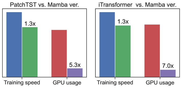
Figure 1: Training speed and GPU comparisons.

The recent popularity of state space models (SSMs; fu2022h3 ; gu2021efficiently ; zhang2023spacetime ) has caught our attention. SSMs are principled sequential models that describe the evolution of states over time using ordinary differential equations, making them naturally suitable for time series modeling. Recently, Mamba gu2023mamba enhances traditional SSMs by introducing selection mechanisms to filter out irrelevant information and reset states along. It also incorporates hardware-aware design for efficient parallel training. Mamba has demonstrated competitive performance compared to Transformers across various domains gu2023mamba ; zhu2024vision ; wang2024state , offering rapid inference and scalability with sequence length.

The inherent sequential and selective nature of Mamba has driven us to validate its performance in LTSF and compare it to Transformer. Initially, we replaced the Transformer Block in two SOTA Transformer-based methods, PatchTST nie2023a and iTransformer liu2023itransformer , with Mamba Block, resulting in corresponding Mamba versions. Subsequently, we compared them with PatchTST and iTransformer, with the results presented in Table 1 and Figure 1. Our findings indicate that, compared to PatchTST and iTransformer, the Mamba versions exhibited a 1.3x faster training speed, with memory consumption reduced by 5.3x and 7.0x, respectively. However, despite these improvements, we did not observe a performance advantage of Mamba over Transformer on these LTSF datasets.

This seems to contradict the intuition that Mamba is naturally more suitable for time series modeling. We made four improvements to Mamba and introduced MambaTS, a framework specifically designed for LTSF based on improved selective SSMs. Firstly, we introduce variable scan along time (VST). Similar to PatchTST nie2023a , we initially segment every variable into patches and linearly map them to tokens. However, unlike PatchTST, we adopt a variable mixing manner by alternately organizing the tokens of different variables at the same timestep, thus expanding them along time to form a global historical look-back window. However, the lack of identified causality among variables results in the locally non-sequential spanning outcomes after VST. In the case, causal convolution in the original Mamba Block may impact on model performance. In addition, some studies have argued that causal convolution for the look-back window is unnecessary and may restrict temporal feature extraction liu2022scinet ; wang2023micn . To address these issues, we introduce the Temporal Mamba Block (TMB) by removing local convolution before SSM. Additionally, to mitigate overfitting, we incorporated a dropout mechanism hinton2012improving into selective parameters of TMB, building on findings that excessive information integration can lead to overfitting nie2023a , as observed in our experiments with Mamba.

While TMB is tailored for temporal modeling, it remains sensitive to scan order, highlighting the significance of variable organization. To address this, we introduce variable permutation training (VPT). By shuffling the variable order in each iteration, we mitigate the impact of undefined variable order and boost the model’s local interaction capacity. An ensuing question is how do we determine the optimal channel scan order? Inspired by topological sorting tarjan1976edge ; prabhumoye2020topological in graph theory, we further propose a novel Variable-Aware Scan along Time (VAST). In VAST, we consider the position of nodes in a linear sequence, such as $a\to c,b\to c$, where a reasonable topological order might be $a\to b\to c$. Specifically, during training, we update a distance matrix that captures variable relationships based on forward propagation results following each permutation. This formulation transforms the optimal scan order problem into an instance of the asymmetric traveling salesman problem (ATSP) in a dense graph. To address this, we utilize a simulated annealing-based ATSP solver to derive the final channel scan order. To our knowledge, we are the first to investigate variable scan order in the context of SSMs for time series modeling.

Through the aforementioned four designs, MambaTS achieves efficient modeling of global dependencies across time and variables with linear complexity. Extensive experiments on eight popular public datasets demonstrate that MambaTS achieve SOTA performance in most LSTF tasks and settings.

In summary, our contributions are as follows:

• We introduce MambaTS, a novel time series forecasting model that builds upon improved selective SSMs. By incorporating VST, we effectively organize historical information of all variables to create a global retrospective sequence.

• We present TMB, which addresses the dispensability of causal convolutions in vanilla Mamba for LTSF. Furthermore, we incorporate a dropout mechanism for the selective parameters of TMB to mitigate model overfitting.

• We implement VPT strategy to eliminate the influence of undefined variable order and further enhance the model’s local context interaction capabilities.

• We propose VAST, which discover relationships between different variables during training and leverages an ATSP solver to determine the optimal variable scan order during inference.

2 Related Work

Long-term time series forecasting

Traditional LTSF methods leverage the statistical properties and patterns of time series data for prediction box1970distribution . In recent years, LTSF has shifted towards deep learning approaches, where various neural networks are utilized to capture complex patterns and dependencies, elevating LTSF performance. These methods can be broadly classified into two categories: variable-mixing and variable-independent. Variable-mixing methods employ diverse architectures to model dependencies across time and variables. RNNs salinas2020deepar ; NIPS2015_07563a3f ; lai2018modeling were initially introduced to LTSF due to the nature of sequence modeling. TCNs, known for their local bias, are effective in capturing local patterns in time series data and have shown promising results in LTSF bai2018empirical ; wang2023micn ; wu2023timesnet . Transformers are subsequently introduced to accomplish long-range dependency modeling through self-attention and have become a mainstream method in LSTF wen2022transformers . However, due to the quadratic complexity, Transformer-based methods have struggled with optimization efficiency zhou2021informer ; liu2021pyraformer ; wu2021autoformer ; zhou2022fedformer ; li2019enhancing . Recently, significant improvements have been made in these methods with patch-based techniques zhang2023crossformer ; nie2023a . MLPs are also commonly used for LTSF and have achieved impressive results with their simple and direct architectures ekambaram2023tsmixer . Graph neural networks have been utilized to model relationships between variables wu2020mtgnn . FourierGNN yi2024fouriergnn represents the entire time series information as a hypervariate graph and employs Fourier Graph Neural Network for global dependency modeling. On the other hand, variable-independent methods focus solely on modeling temporal dependencies under the assumption of variable independence Zeng2023Dlinear ; nie2023a ; zhou2023one . These approaches are known for their simplicity and efficiency, often capable of mitigating model overfitting and achieving remarkable outcomes Zeng2023Dlinear ; nie2023a . Nevertheless, this assumption may oversimplify the problem and potentially lead to ill-posed scenarios zhang2023crossformer .

State Space Models

Recently, some works box1970distribution have combined SSMs kalman1960new with deep learning and demonstrated significant potential in addressing the long-range dependencies problem. However, the prohibitive computation and memory requirements of state representations often hinder their practical applications gu2021efficiently . Several efficient variants of SSMs, such as S4 gu2021efficiently , H3 fu2022h3 , Gated State Space mehta2022long , and RWKV peng2023rwkv , have been proposed to enhance model performance and efficiency in practical tasks. Mamba gu2023mamba addresses a key limitation of traditional SSMs methods by introducing a data-dependent selection mechanism based on S4 to efficiently filter specific inputs and capture long-range context that scales with sequence length. Mamba demonstrates linear-time efficiency in modeling long sequences and surpasses Transformer models in benchmark evaluations gu2023mamba .

Mamba has also been successfully extended to non-sequential data such as image liu2024vmamba ; zhu2024vision ; wang2024state , point cloud liang2024pointmamba , table ahamed2024mambatab and graphs wang2024graph ; behrouz2024graph to enhance its capability in capturing long-range dependencies. To address the scan order sensitivity of Mamba, some studies have introduced bidirectional scanning zhu2024vision , multi-directional scanning li2024mamba ; liu2024vmamba , and even automatic direction scanning huang2024localmamba . However, there is currently limited work considering the issue of variable scan order in temporal problems. To tackle this challenge, we introduce the VAST strategy to further enhance the expressive power of MambaTS. Similar to our approach, Graph-Mamba wang2024graph also proposes a similar permutation strategy to extend context-aware reasoning on graphs. However, it is based on node prioritization, introducing a biased strategy specifically designed for graphs.

3 Preliminaries

State Space Models

SSMs are typically regarded as linear time-invariant (LTI) systems that map continuous input signals $x(t)$ to corresponding outputs $y(t)$ through a state representation $h(t)$. This state space describes the evolution of the state over time and can be represented using ordinary differential equations as follows:

$$h^{\prime}(t) =\bm{A}h(t)+\bm{B}x(t)$$ (1)

$$y(t) =\bm{C}h(t)+\bm{D}x(t)$$

Here, $h^{\prime}(t)=\frac{dh(t)}{dt}$, and $\bm{A},\bm{B},\bm{C}$, and $\bm{D}$ are parameters of the time-independent SSMs.

Discretization

Finding analytical solutions for SSMs is highly challenging due to their continuous nature. Discretization is typically employed to facilitate analysis and solution in the discrete domain, which involves approximating the continuous-time state space model into a discrete-time representation. This is done by sampling the input signals at fixed time intervals to obtain their discrete-time counterparts. The resulting discrete-time state space model can be represented as:

$$h_{k} =\overline{\bm{A}}h_{k-1}+\overline{\bm{B}}x_{k}$$ (2)

$$y_{k} =\overline{\bm{C}}h_{k}+\overline{\bm{D}}x_{k}$$

Here, $h_{k}$ represents the state vector at time instant $k$, and $x_{k}$ represents the input vector at time instant $k$. The matrices $\overline{A}$ and $\overline{B}$ are derived from the continuous-time matrices $A$ and $B$ using appropriate discretization techniques such as the Euler or ZOH (Zero-Order Hold) method. In this case, $\overline{\bm{A}}=\exp(\Delta\bm{A}),\overline{\bm{B}}=(\Delta\bm{A})^{-1}(\exp(\Delta\bm{A})-\bm{I})\cdot\Delta\bm{B}$.

Selective Scan Mechanism

Mamba further introduces selective SSMs by allowing the parameters to influence the interactions along the sequence in a context-dependent manner. This selective mechanism enables Mamba to filter out irrelevant noise in time series tasks, while selectively propagating or forgetting information relevant to the current input. This differs from previous SSMs methods with static parameters, but it does break the LTI characteristics. Therefore, Mamba takes a hardware optimization approach and implements parallel scan training to address this challenge.

4 Model architecture

For the multivariate time series prediction problem, given an $L$-length look-back window time series data with $K$ variables $(\mathbf{x}_{1},\mathbf{x}_{2},\cdots,\mathbf{x}_{L})$, where $\mathbf{x}_{i}\in\mathbb{R}^{K}$ represents the values of $K$ variables at time step $i$. Our objective is to forecast the values of the future $T$ time steps, denoted as $(\mathbf{x}_{L+1},\cdots,\mathbf{x}_{L+2},\cdots,\mathbf{x}_{L+T})$.

4.1 Overall Architecture

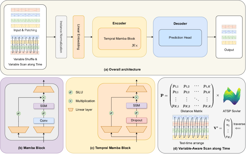
Figure 2: The overall architecture of MambaTS.

The architecture of MambaTS is illustrated in Figure 2. It primarily consists of an embedding layer, an instance normalization layer, $N\times$ Temporal Mamba blocks, and a prediction head.

Patching and Tokenization

Semantic information at a single time point tends to be sparse. Following PatchTST nie2023a , we segment each variable into about $M=L/s$ patches every $s$ time steps, aggregate information from neighboring points, and then map them to a $D$-dimensional token through linear mapping. This process efficiently reduces memory usage and eliminates redundant information.

Variable Scan along Time

By embedding $K$ variables, we derive $K\times M$ tokens. To fully leverage the linear complexity and selective advantages of Mamba while establishing a comprehensive representation of the look-back window, we introduce the variable scan along time mechanism. VST arranges tokens of variables at each time step in an alternating fashion temporally. This structured organization enables the model to more accurately capture long-term dependencies and dynamic changes in time series data. Subsequently, we feed the results of VST into the encoder.

Encoder

The encoder consists of $N$ stacked TMBs, each comprising two branches. The right SSM branch focuses on sequence modeling, while the left branch contains a gated non-linear layer. The computation process of the original Mamba block is as follows:

$$h_{t}=\text{SSM}(\text{Conv}(\text{Linear}(\mathbf{x_{t}})))+\sigma(\text{Linear}(\mathbf{x_{t}})).$$ (3)

Here, causal convolution, acting as a shift-SSM, is inserted before the SSM module to enhance connections between adjacent tokens, as depicted in Figure 2 (b). However, the results generated by VST may not be causal locally. Therefore, TMB (see Figure 2 (c)) removes this component. Additionally, to prevent overfitting, we introduce a dropout mechanism hinton2012improving for the selective parameters, as follows:

$$h_{t}=\text{SSM}(\text{Dropout}(\text{Linear}(\mathbf{x_{t}})))+\sigma(\text{Linear}(\mathbf{x_{t}})).$$ (4)

Prediction Head

Since the encoder is capable of capturing global dependencies, for efficiency reasons, similar to PatchTST nie2023a , we adopt a channel-independent decoding approach in the decoding phase. Each channel is decoded individually using a simple linear head.

Instance Normalization

To mitigate distribution shift between training and test data, following RevIN kim2021reversible , we standardize each input channel to zero mean and unit standard deviation, and keep track of these statistics for de-normalization of the model prediction.

Loss Function

We choose mean squared error (MSE) loss as the primary loss function, given by:

$$\mathcal{L}=\mathbb{E}_{\mathbf{x}}\frac{1}{M}\sum_{i=1}^{M}\left\|\hat{\mathbf{x}}_{L+1:L+T}^{(i)}-\mathbf{x}_{L+1:L+T}^{(i)}\right\|_{2}^{2}.$$ (5)

4.2 Variable Permutation Training

To mitigate the impact of undefined channel orders and augment local context interactions, we introduce the variable permutation training (VPT) strategy. Specifically, for the encoder input consisting of $K\times M$ tokens, VPT shuffle the $K$ tokens at each time step in a consistent order, and revert the shuffle state after decoding to ensure the correct output of the sequence.

4.3 Variable-Aware Scan along Time

To determine the optimal variable scan order, it is essential to consider the relationships between variables. However, since these relationships are unknown, we propose VAST, a simple yet effective method to estimate variable relationships, guiding the scan order during inference stage.

Training

For any $K$ variables, we maintain a directed graph adjacency matrix $\bm{P}\in\mathbb{R}^{K\times K}$, where $p_{i,j}$ represents the cost from node $i$ to node $j$. Notably, with the introduction of variable permutation during training, we can explore various combinations of scan orders and evaluate their effectiveness using Eq. (5). Following a permutation, a node index sequence $\mathbf{V}=\{v_{1},v_{2},\cdots,v_{K}\}$ is obtained, where $v_{k}$ denotes the new index in the shuffled sequence. Subsequently, $K-1$ transition tuples $\{(v_{1},v_{2}),(v_{2},v_{3}),\cdots(v_{K-1},v_{K})\}$ are derived. For each sample, a training loss ${l}^{(t)}$ is computed during the $t$-th iteration of the network. Therefore, we update $\bm{P}$ with exponential moving average:

$$p^{(t)}_{v_{k},v_{k+1}}=\beta p^{(t-1)}_{v_{k},v_{k+1}}+(1-\beta)l^{(t)},$$ (6)

where $\beta$ is a hyperparameter that controls the rate of the moving average, determining the impact of new estimates on the variable relationships. To facilitate efficient training, we extend Eq. (6) to a batch version. By a simple centralization operation to eliminate the influence of different sample batches, i.e., $\bar{l}^{(t)}={l}^{(t)}-\mu({l}^{(t)})$, where $\mu$ is the mean function, the equation is modified to:

$$p^{(t)}_{v_{k},v_{k+1}}=\beta p^{(t-1)}_{v_{k},v_{k+1}}+(1-\beta)\bar{l}^{(t)}.$$ (7)

Inference

Throughout training, $\bm{P}$ are leveraged to determine the optimal variable scan order. This involves solving the asymmetric traveling salesman problem, which seeks the shortest path visiting all nodes. Given the dense connectivity represented by $\bm{P}$, finding the optimal traversal path is NP-hard. Hence, we introduce a heuristic-based simulated annealing dreo2006metaheuristics algorithm for path decoding.

5 Experiments

Table 2: Summary of Dataset Characteristics

Datasets ETTh2 ETTm2 Weather Electricity Traffic Solar Covid-19 PEMS Features 7 7 21 321 862 137 948 358 Time steps 17,420 17,420 52,696 26,304 17,544 52,179 1,392 21,351 Frequency 1 hour 15 mins 10 mins 1 hour 1 hour 10 mins 1 day 5 mins

Dataset

We conducted extensive experiments on eight public datasets, as shown in Table 2, including two ETT datasets zhou2021informer , Weather, Electricity, Traffic wu2021autoformer , Solar lai2018modeling , Covid-19 panagopoulos2021transfer , and PEMS liu2022scinet , covering domains such as electricity, energy, transportation, weather, and health.

Baselines and metrics

To demonstrate the effectiveness of MambaTS, we compared it against SOTA models of LTSF, including five popular Transformer-based methods: PatchTST nie2023a , iTransformer liu2023itransformer , FEDformer zhou2022fedformer , Autoformer wu2021autoformer , and three competitive non-Transformer-based methods: DLinear Zeng2023Dlinear , MICN wang2023micn , and FourierGNN yi2024fouriergnn . Following PatchTST nie2023a , we primarily evaluate the models using Mean Squared Error (MSE) and Mean Absolute Error (MAE).

Implementation Details

Experiments were performed on an NVIDIA RTX 3090 Ti 24 GB GPU using the Adam optimizer kingma2014adam with betas of (0.9, 0.999). Training ran for 10 epochs with early stopping implemented using a patience of 3 to avoid overfitting. The best parameter selection for all comparison models was carefully tuned on the validation set.

Table 3: Multivariate long-term series forecasting results. All models employ a look-back window length of $L=96$ for the Covid-19 dataset and $L=720$ for the remaining datasets.

Models MambaTS (ours) PatchTST (2023) iTransformer (2023) DLinear (2023) MICN (2023) FourierGNN (2023) FEDformer (2022) Autoformer (2021) Metric MSE MAE MSE MAE MSE MAE MSE MAE MSE MAE MSE MAE MSE MAE MSE MAE ETTh2 96 0.283 0.349 0.283 0.347 0.312 0.363 0.306 0.370 0.289 0.354 0.454 0.481 0.332 0.374 0.332 0.368 192 0.356 0.397 0.354 0.391 0.384 0.408 0.411 0.437 0.408 0.444 0.560 0.541 0.407 0.446 0.426 0.434 336 0.370 0.416 0.376 0.411 0.431 0.444 0.542 0.514 0.547 0.516 0.608 0.568 0.400 0.447 0.477 0.479 720 0.407 0.446 0.402 0.440 0.432 0.463 0.900 0.671 0.834 0.688 0.820 0.648 0.412 0.469 0.453 0.490 ETTm2 96 0.174 0.269 0.168 0.259 0.181 0.275 0.163 0.258 0.177 0.274 0.229 0.327 0.180 0.271 0.205 0.293 192 0.235 0.309 0.237 0.309 0.243 0.315 0.222 0.304 0.236 0.310 0.308 0.384 0.252 0.318 0.278 0.336 336 0.288 0.346 0.279 0.336 0.297 0.352 0.274 0.336 0.299 0.350 0.362 0.413 0.324 0.364 0.343 0.379 720 0.360 0.393 0.363 0.390 0.381 0.404 0.407 0.432 0.421 0.434 0.482 0.487 0.410 0.420 0.414 0.419 Weather 96 0.145 0.196 0.149 0.198 0.180 0.232 0.168 0.227 0.167 0.231 0.162 0.232 0.238 0.314 0.249 0.329 192 0.193 0.241 0.194 0.241 0.228 0.270 0.212 0.267 0.212 0.271 0.207 0.276 0.275 0.329 0.325 0.370 336 0.246 0.283 0.245 0.282 0.291 0.316 0.256 0.305 0.275 0.337 0.261 0.318 0.339 0.377 0.351 0.391 720 0.314 0.331 0.314 0.334 0.354 0.359 0.315 0.355 0.312 0.349 0.336 0.366 0.389 0.409 0.415 0.426 Electricity 96 0.128 0.223 0.130 0.223 0.133 0.229 0.133 0.230 0.151 0.260 0.166 0.274 0.186 0.302 0.196 0.313 192 0.146 0.239 0.147 0.240 0.155 0.251 0.147 0.244 0.165 0.276 0.182 0.289 0.197 0.311 0.211 0.324 336 0.161 0.258 0.164 0.257 0.167 0.264 0.162 0.261 0.183 0.291 0.201 0.308 0.213 0.328 0.214 0.327 720 0.187 0.283 0.203 0.292 0.194 0.288 0.196 0.294 0.201 0.312 0.235 0.339 0.233 0.344 0.236 0.342 Traffic 96 0.347 0.247 0.367 0.253 0.349 0.255 0.385 0.269 0.445 0.295 0.494 0.303 0.576 0.359 0.597 0.371 192 0.357 0.255 0.382 0.259 0.359 0.263 0.395 0.273 0.461 0.302 0.513 0.310 0.610 0.380 0.607 0.382 336 0.372 0.262 0.396 0.267 0.379 0.272 0.409 0.281 0.483 0.307 0.534 0.320 0.608 0.375 0.623 0.387 720 0.416 0.284 0.433 0.287 0.417 0.291 0.449 0.305 0.527 0.310 0.597 0.346 0.621 0.375 0.639 0.395 Solar 96 0.165 0.232 0.185 0.246 0.170 0.246 0.191 0.257 0.190 0.243 0.183 0.232 0.214 0.311 0.316 0.369 192 0.179 0.242 0.201 0.262 0.195 0.263 0.211 0.273 0.205 0.247 0.198 0.256 0.281 0.364 0.418 0.437 336 0.191 0.253 0.209 0.266 0.217 0.282 0.228 0.285 0.219 0.250 0.205 0.261 0.294 0.378 0.438 0.467 720 0.200 0.261 0.226 0.283 0.208 0.276 0.236 0.294 0.227 0.263 0.202 0.265 0.315 0.406 0.618 0.550 Covid-19 12 0.774 0.036 1.236 0.054 0.998 0.046 2.643 0.087 6.505 0.110 3.584 0.075 7.607 0.316 7.695 0.406 24 1.151 0.048 1.584 0.064 1.488 0.060 3.678 0.100 23.587 0.155 2.532 0.079 8.162 0.312 8.253 0.410 48 1.964 0.068 2.639 0.089 2.505 0.082 5.836 0.131 33.467 0.206 12.922 0.140 9.458 0.328 9.563 0.440 96 4.108 0.106 11.811 0.176 6.435 0.146 10.092 0.185 24.247 0.261 7.991 0.164 12.694 0.550 12.592 0.456 PEMS 12 0.060 0.162 0.063 0.166 0.064 0.167 0.078 0.187 0.094 0.204 0.091 0.202 0.283 0.394 0.584 0.607 24 0.076 0.180 0.080 0.185 0.081 0.187 0.113 0.224 0.116 0.229 0.116 0.232 0.300 0.431 0.672 0.664 48 0.102 0.207 0.109 0.213 0.111 0.215 0.167 0.274 0.147 0.255 0.165 0.271 0.396 0.476 0.879 0.781 96 0.134 0.232 0.145 0.243 0.142 0.240 0.212 0.313 0.256 0.362 0.196 0.300 0.477 0.537 1.100 0.895

Table 4: Ablations on components. VST: Variable Scan along Time. TMB: Temporal Mamba Block. VAST: Variable-Aware Scan along Time. The average results of all predicted lengths are listed here.

VST	TMB	VAST	ETTm2		Traffic		Electricity		Solar
			MSE	MAE	MSE	MAE	MSE	MAE	MSE	MAE
$\Circle$	$\Circle$	$\Circle$	0.285	0.342	0.400	0.273	0.167	0.260	0.192	0.261
$\CIRCLE$	$\Circle$	$\Circle$	0.284	0.341	0.383	0.268	0.164	0.260	0.197	0.266
$\Circle$	$\CIRCLE$	$\Circle$	0.264	0.329	0.389	0.268	0.160	0.255	0.191	0.253
$\CIRCLE$	$\CIRCLE$	$\Circle$	0.263	0.327	0.376	0.267	0.161	0.257	0.193	0.261
$\CIRCLE$	$\CIRCLE$	$\CIRCLE$	0.262	0.325	0.373	0.262	0.155	0.251	0.184	0.247

5.1 Main results

Table 3 displays the results of multivariate long-term forecasting. Overall, MambaTS achieved new SOTA results (highlighted in red bold) across various prediction horizons on most datasets. While DLinear and PatchTST assume variable independence and perform well on datasets with a small number of variables like ETTh2/m2 ($K=7$) and Weather ($K=21$), their performance diminishes on complex datasets with a larger number of variables such as Traffic ($K=862$) and Covid-19 ($K=948$), highlighting the limitations of the variable-independent assumption. Conversely, iTransformer exhibited contrasting performance, excelling on intricate datasets but underperforming on datasets with fewer variables. Other baselines demonstrated competitive results on specific datasets under certain prediction scenarios.

5.2 Ablation studies and analyses

To validate the rationality and effectiveness of the proposed components, we conducted extensive ablation experiments as shown in Table 4, Table 5, Figure 3 and Figure 4.

Component Ablation

Table 4 presents the ablation on components. Initially, integrating VST with the baseline Mamba-based PatchTST led to performance improvements across most datasets, showcasing the benefits of considering all variables. Substituting solely with TMB resulted in a notable performance boost, underscoring the efficacy of TMB for temporal modeling. Combining VST and TMB yielded performance superior to VST alone but slightly below the original TMB, attributed to VST including all variables while TMB removes local bias causal convolutions, making it more sensitive to variable order. However, this issue is addressed by introducing VAST (see Table 4, row 4). Through these components, MambaTS achieves optimal performance.

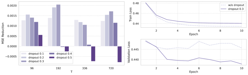
Figure 3: Dropout ablations of TMB. Left: TMB with varying dropout rates on Weather dataset. Right: Loss curves over training.

Dropout Ablation

We further analyzed the role of the dropout in TMB. Figure 3 (left) shows the results of MambaTS with different dropout rates (0.1-0.5) on the Weather dataset. Compared to no dropout, the reduction in MSE of MambaTS increased with the dropout rate, achieving the best performance at 0.2 and 0.3, and performance degradation beyond 0.4. Figure 3 (right) illustrates corresponding loss curves during training, indicating that the dropout in TMB helps prevent premature convergence and overfitting. Additionally, we observed that dropout facilitated lower validation loss.

VAST Ablation

In Table 5, we conducted extensive ablation studies on the VAST strategy, focusing on the design and selection of path decoding strategies. "W/o VPT" in Table 5 indicates that MambaTS was trained without VPT as the baseline. "Random (100x)" represents sampling 100 test runs after training with VPT and averaging the results. It can be observed that "Random (100x)" significantly outperformed "W/o VPT", which underscores the effectiveness of VPT. Further visual comparisons in Figure 4 show that even random variable scanning outperforms "W/o VPT" in most cases. We then explored different heuristic decoding strategies, including Greedy Strategy (GD), Local Search (LS), Lin and Lernighan (LK), and Simulated Annealing (SA). We defaulted to adopting SA as our solver. As a trade-off between efficiency and performance, we did not employ an exact ATSP solver due to its exponential complexity. As shown in Table 5 and Figure 4, SA consistently outperformed other solvers in terms of relative performance consistency.

Scanning	ETTm2		Traffic		Electricity
	MSE	MAE	MSE	MAE	MSE	MAE
W/o VPT	0.263	0.327	0.376	0.267	0.161	0.257
Random (100x)	0.262	0.326	0.374	0.265	0.158	0.256
VAST (GD.)	0.260	0.322	0.376	0.267	0.161	0.257
VAST (LS.)	0.261	0.325	0.375	0.265	0.157	0.254
VAST (LK.)	0.262	0.325	0.374	0.264	0.156	0.252
VAST (SA.)	0.259	0.321	0.373	0.262	0.156	0.251

Table 5: Ablations on VAST.

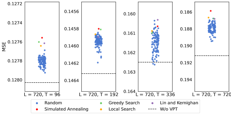
Figure 4: Sampling results of VAST. Employing swarm plot to prevent overlapping points (better in color).

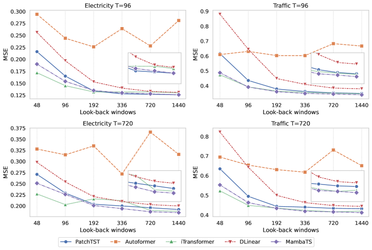
Figure 5: Performance of MambaTS in different datasets with varying length look-back windows.

Table 6: Computational complexity analysis. SA: Self-attention. Conv: Convolution.

Method Temporal mixing Variable mixing Computational complexity Autoformer SA MLP $\mathcal{O}(L\log L)$ FEDformer SA MLP $\mathcal{O}(L)$ MICN Conv Conv $\mathcal{O}(K^{2}L)$ FourierGNN GNN GNN $\mathcal{O}(KL)$ DLinear MLP – $\mathcal{O}(L)$ PatchTST SA – $\mathcal{O}\left(\left(\frac{L}{P}\right)^{2}\right)$ iTransformer MLP SA $\mathcal{O}(K^{2})$ MambaTS TMB TMB $\mathcal{O}\left(\frac{KL}{P}\right)$

5.3 Model Analysis

Increasing Lookback Window

Previous studies have shown that Transformer-based methods may not necessarily benefit from a growing lookback window Zeng2023Dlinear ; nie2023a , possibly due to distracted attention over the long input. In Figure 5, we assess MambaTS’s performance in this context and compare it with several baselines. It can be observed that MambaTS consistently demonstrates the ability to benefit from the growing input sequence. iTransformer, PatchTST, and DLinear also show this benefit, but MambaTS’s overall curve is lower than PatchTST and DLinear. Compared to iTransformer, MambaTS benefits more from a longer lookback window. Additionally, we notice that iTransformer seems to exhibit discontinuous gains on individual dataset tasks.

Efficiency Analysis

MambaTS integrates historical information from all variables using VST and conducts global dependency modeling through TMB. The computational complexity of MambaTS is $\mathcal{O}(\frac{KL}{P})$, where $K$ represents the number of variables, $L$ denotes the length of the lookback window, and $P$ signifies the patch stride. Table 6 outlines the computational complexity of other models.

Among them, Autoformer and FEDformer employ traditional point-wise tokenization, with computational complexity dependent on $L$. MICN and FourierGNN, focusing on modeling dependencies between variables, entail higher complexity. DLinear achieves $\mathcal{O}(L)$ complexity but lacks variable mixing. PatchTST and iTransformer have complexities of $\mathcal{O}(\left(\frac{L}{P}\right)^{2})$ and $\mathcal{O}(K^{2})$, respectively. In contrast, MambaTS’s complexity of $\mathcal{O}(K\cdot\frac{L}{P})$ strikes a balance between these approaches, as illustrated in Table 3, highlighting the meaningful and efficient equilibrium.

6 Conclusion

In this work, we present MambaTS, a novel multivariate time series forecasting model built upon improved selective SSMs. We first introduce VST to organize the historical information of all variables, forming a global retrospective sequence. Recognizing the dispensability of causal convolution in Mamba for LTSF, we propose the Temporal Mamba Block. Furthermore, we enhance Mamba’s selective parameters with dropout regularization to prevent overfitting and enhance model performance. To mitigate the scan order sensitivity problem, we implement variable permutation training to counter the impact of undefined variables order. Lastly, we propose VAST to dynamically discover relationships between variables during training and solve the shortest path visiting problem using an ATSP solver to determine the optimal variable scann order. Through these designs, MambaTS achieves global dependency modeling with linear complexity and establishes new state-of-the-art results across multiple datasets and prediction settings.

References

- (1) Bryan Lim and Stefan Zohren. Time-series forecasting with deep learning: a survey. Philosophical Transactions of the Royal Society A, 379(2194):20200209, 2021.
- (2) Qingsong Wen, Tian Zhou, Chaoli Zhang, Weiqi Chen, Ziqing Ma, Junchi Yan, and Liang Sun. Transformers in time series: A survey. arXiv preprint arXiv:2202.07125, 2022.
- (3) Xiangfei Qiu, Jilin Hu, Lekui Zhou, Xingjian Wu, Junyang Du, Buang Zhang, Chenjuan Guo, Aoying Zhou, Christian S Jensen, Zhenli Sheng, et al. Tfb: Towards comprehensive and fair benchmarking of time series forecasting methods. arXiv preprint arXiv:2403.20150, 2024.
- (4) Shaojie Bai, J Zico Kolter, and Vladlen Koltun. An empirical evaluation of generic convolutional and recurrent networks for sequence modeling. arXiv preprint arXiv:1803.01271, 2018.
- (5) Rajat Sen, Hsiang-Fu Yu, and Inderjit S Dhillon. Think globally, act locally: A deep neural network approach to high-dimensional time series forecasting. In Advances in Neural Information Processing Systems (NeurIPS), 2019.
- (6) Ashish Vaswani, Noam Shazeer, Niki Parmar, Jakob Uszkoreit, Llion Jones, Aidan N Gomez, Łukasz Kaiser, and Illia Polosukhin. Attention is all you need. In Advances in Neural Information Processing Systems (NeurIPS), volume 30, 2017.
- (7) Haoyi Zhou, Shanghang Zhang, Jieqi Peng, Shuai Zhang, Jianxin Li, Hui Xiong, and Wancai Zhang. Informer: Beyond efficient transformer for long sequence time-series forecasting. Proceedings of the AAAI Conference on Artificial Intelligence, 35(12):11106–11115, May 2021.
- (8) Yuqi Nie, Nam H Nguyen, Phanwadee Sinthong, and Jayant Kalagnanam. A time series is worth 64 words: Long-term forecasting with transformers. In International Conference on Learning Representations (ICLR), 2023.
- (9) Haixu Wu, Jiehui Xu, Jianmin Wang, and Mingsheng Long. Autoformer: Decomposition transformers with auto-correlation for long-term series forecasting. In Advances in Neural Information Processing Systems (NeurIPS), 2021.
- (10) Tian Zhou, Ziqing Ma, Qingsong Wen, Xue Wang, Liang Sun, and Rong Jin. Fedformer: Frequency enhanced decomposed transformer for long-term series forecasting. In International Conference on Machine Learning (ICML), 2022.
- (11) Shiyang Li, Xiaoyong Jin, Yao Xuan, Xiyou Zhou, Wenhu Chen, Yu-Xiang Wang, and Xifeng Yan. Enhancing the locality and breaking the memory bottleneck of transformer on time series forecasting. In Advances in Neural Information Processing Systems (NeurIPS), 2019.
- (12) Yong Liu, Tengge Hu, Haoran Zhang, Haixu Wu, Shiyu Wang, Lintao Ma, and Mingsheng Long. itransformer: Inverted transformers are effective for time series forecasting. arXiv preprint arXiv:2310.06625, 2023.
- (13) Ailing Zeng, Muxi Chen, Lei Zhang, and Qiang Xu. Are transformers effective for time series forecasting? Proceedings of the AAAI Conference on Artificial Intelligence, 37(9):11121–11128, Jun. 2023.
- (14) Daniel Y Fu, Tri Dao, Khaled K Saab, Armin W Thomas, Atri Rudra, and Christopher Ré. Hungry hungry hippos: Towards language modeling with state space models. arXiv preprint arXiv:2212.14052, 2022.
- (15) Albert Gu, Karan Goel, and Christopher Ré. Efficiently modeling long sequences with structured state spaces. arXiv preprint arXiv:2111.00396, 2021.
- (16) Michael Zhang, Khaled K Saab, Michael Poli, Tri Dao, Karan Goel, and Christopher Ré. Effectively modeling time series with simple discrete state spaces. arXiv preprint arXiv:2303.09489, 2023.
- (17) Albert Gu and Tri Dao. Mamba: Linear-time sequence modeling with selective state spaces. arXiv preprint arXiv:2312.00752, 2023.
- (18) Lianghui Zhu, Bencheng Liao, Qian Zhang, Xinlong Wang, Wenyu Liu, and Xinggang Wang. Vision mamba: Efficient visual representation learning with bidirectional state space model. arXiv preprint arXiv:2401.09417, 2024.
- (19) Xiao Wang, Shiao Wang, Yuhe Ding, Yuehang Li, Wentao Wu, Yao Rong, Weizhe Kong, Ju Huang, Shihao Li, Haoxiang Yang, et al. State space model for new-generation network alternative to transformers: A survey. arXiv preprint arXiv:2404.09516, 2024.
- (20) Minhao Liu, Ailing Zeng, Muxi Chen, Zhijian Xu, Qiuxia Lai, Lingna Ma, and Qiang Xu. Scinet: Time series modeling and forecasting with sample convolution and interaction. Advances in Neural Information Processing Systems, 35:5816–5828, 2022.
- (21) Huiqiang Wang, Jian Peng, Feihu Huang, Jince Wang, Junhui Chen, and Yifei Xiao. MICN: Multi-scale local and global context modeling for long-term series forecasting. In International Conference on Learning Representations (ICLR), 2023.
- (22) Geoffrey E Hinton, Nitish Srivastava, Alex Krizhevsky, Ilya Sutskever, and Ruslan R Salakhutdinov. Improving neural networks by preventing co-adaptation of feature detectors. arXiv preprint arXiv:1207.0580, 2012.
- (23) Robert Endre Tarjan. Edge-disjoint spanning trees and depth-first search. Acta Informatica, 6(2):171–185, 1976.
- (24) Shrimai Prabhumoye, Ruslan Salakhutdinov, and Alan W Black. Topological sort for sentence ordering. In Proceedings of the 58th Annual Meeting of the Association for Computational Linguistics, pages 2783–2792, 2020.
- (25) George EP Box and David A Pierce. Distribution of residual autocorrelations in autoregressive-integrated moving average time series models. Journal of the American statistical Association, 65(332):1509–1526, 1970.
- (26) David Salinas, Valentin Flunkert, Jan Gasthaus, and Tim Januschowski. Deepar: Probabilistic forecasting with autoregressive recurrent networks. International Journal of Forecasting, 36(3):1181–1191, 2020.
- (27) Xingjian SHI, Zhourong Chen, Hao Wang, Dit-Yan Yeung, Wai-kin Wong, and Wang-chun WOO. Convolutional lstm network: A machine learning approach for precipitation nowcasting. In Advances in Neural Information Processing Systems (NeurIPS), volume 28, 2015.
- (28) Guokun Lai, Wei-Cheng Chang, Yiming Yang, and Hanxiao Liu. Modeling long-and short-term temporal patterns with deep neural networks. In The 41st international ACM SIGIR conference on research & development in information retrieval, pages 95–104, 2018.
- (29) Haixu Wu, Tengge Hu, Yong Liu, Hang Zhou, Jianmin Wang, and Mingsheng Long. Timesnet: Temporal 2d-variation modeling for general time series analysis. In International Conference on Learning Representations (ICLR), 2023.
- (30) Shizhan Liu, Hang Yu, Cong Liao, Jianguo Li, Weiyao Lin, Alex X Liu, and Schahram Dustdar. Pyraformer: Low-complexity pyramidal attention for long-range time series modeling and forecasting. In International Conference on Learning Representations (ICLR), 2021.
- (31) Yunhao Zhang and Junchi Yan. Crossformer: Transformer utilizing cross-dimension dependency for multivariate time series forecasting. In International Conference on Learning Representations (ICLR), 2023.
- (32) Vijay Ekambaram, Arindam Jati, Nam Nguyen, Phanwadee Sinthong, and Jayant Kalagnanam. Tsmixer: Lightweight mlp-mixer model for multivariate time series forecasting. In Proceedings of the 29th ACM SIGKDD Conference on Knowledge Discovery and Data Mining, pages 459–469, 2023.
- (33) Zonghan Wu, Shirui Pan, Guodong Long, Jing Jiang, Xiaojun Chang, and Chengqi Zhang. Connecting the dots: Multivariate time series forecasting with graph neural networks. In Proceedings of the 26th ACM SIGKDD international conference on knowledge discovery & data mining, pages 753–763, 2020.
- (34) Kun Yi, Qi Zhang, Wei Fan, Hui He, Liang Hu, Pengyang Wang, Ning An, Longbing Cao, and Zhendong Niu. Fouriergnn: Rethinking multivariate time series forecasting from a pure graph perspective. Advances in Neural Information Processing Systems, 36, 2024.
- (35) Tian Zhou, Peisong Niu, Liang Sun, Rong Jin, et al. One fits all: Power general time series analysis by pretrained lm. Advances in neural information processing systems, 36:43322–43355, 2023.
- (36) Rudolph Emil Kalman. A new approach to linear filtering and prediction problems. 1960.
- (37) Harsh Mehta, Ankit Gupta, Ashok Cutkosky, and Behnam Neyshabur. Long range language modeling via gated state spaces. arXiv preprint arXiv:2206.13947, 2022.
- (38) Bo Peng, Eric Alcaide, Quentin Anthony, Alon Albalak, Samuel Arcadinho, Huanqi Cao, Xin Cheng, Michael Chung, Matteo Grella, Kranthi Kiran GV, et al. Rwkv: Reinventing rnns for the transformer era. arXiv preprint arXiv:2305.13048, 2023.
- (39) Yue Liu, Yunjie Tian, Yuzhong Zhao, Hongtian Yu, Lingxi Xie, Yaowei Wang, Qixiang Ye, and Yunfan Liu. Vmamba: Visual state space model. arXiv preprint arXiv:2401.10166, 2024.
- (40) Dingkang Liang, Xin Zhou, Xinyu Wang, Xingkui Zhu, Wei Xu, Zhikang Zou, Xiaoqing Ye, and Xiang Bai. Pointmamba: A simple state space model for point cloud analysis. arXiv preprint arXiv:2402.10739, 2024.
- (41) Md Atik Ahamed and Qiang Cheng. Mambatab: A simple yet effective approach for handling tabular data. arXiv preprint arXiv:2401.08867, 2024.
- (42) Chloe Wang, Oleksii Tsepa, Jun Ma, and Bo Wang. Graph-mamba: Towards long-range graph sequence modeling with selective state spaces. arXiv preprint arXiv:2402.00789, 2024.
- (43) Ali Behrouz and Farnoosh Hashemi. Graph mamba: Towards learning on graphs with state space models. arXiv preprint arXiv:2402.08678, 2024.
- (44) Shufan Li, Harkanwar Singh, and Aditya Grover. Mamba-nd: Selective state space modeling for multi-dimensional data. arXiv preprint arXiv:2402.05892, 2024.
- (45) Tao Huang, Xiaohuan Pei, Shan You, Fei Wang, Chen Qian, and Chang Xu. Localmamba: Visual state space model with windowed selective scan. arXiv preprint arXiv:2403.09338, 2024.
- (46) Taesung Kim, Jinhee Kim, Yunwon Tae, Cheonbok Park, Jang-Ho Choi, and Jaegul Choo. Reversible instance normalization for accurate time-series forecasting against distribution shift. In International Conference on Learning Representations (ICLR), 2021.
- (47) Johann Dréo, Alain Pétrowski, Patrick Siarry, and Eric Taillard. Metaheuristics for hard optimization: methods and case studies. Springer Science & Business Media, 2006.
- (48) George Panagopoulos, Giannis Nikolentzos, and Michalis Vazirgiannis. Transfer graph neural networks for pandemic forecasting. In Proceedings of the AAAI Conference on Artificial Intelligence, volume 35, pages 4838–4845, 2021.
- (49) Diederik P Kingma and Jimmy Ba. Adam: A method for stochastic optimization. arXiv preprint arXiv:1412.6980, 2014.