Analysis of Cosmic Evolution admitting Garcia-Salcedo Ghost and Generalized Ghost Dark Energy Models
Abstract
This study aims to explore the Garcia-Salcedo ghost dark energy and generalized ghost dark energy models in the context of theory, where is the Ricci scalar and is the self-contraction of stress-energy tensor. We investigate the non-interacting case only corresponding to flat Friedmann-Robertson-Walker universe. We reconstruct the corresponding gravity models using the considered dark energy models by taking two particular models of this gravity. The stability analysis is performed for all the cases. The behavior of the equation of state parameter is also checked. It is found that some of the reconstructed models successfully describe both the phantom and quintessence epochs of the universe, which support the current cosmic accelerated expansion. This exploration reveals the intricate connections between dark energy models and modified gravitational theory, providing significant understanding into the dynamics of the cosmos on a large scale.
Keywords: Reconstruction technique; Modified theory; Dark
energy models; Stability.
PACS: 04.50.Kd; 98.80.-k; 95.36.+x.
1 Introduction
Various cosmic observations such as supernova type-Ia, cosmic microwave background radiations and large-scale structures indicate that the universe is currently expanding. Scientists believe that this expansion is caused by a mysterious force called dark energy (DE), which is characterized by a large negative pressure. Several alternative techniques have been formulated to comprehend the impact of DE on the ongoing cosmic acceleration. Recently, researchers introduced a new DE model called ghost dark energy (GDE) model, based on the dynamics of quantum chromodynamics (QCD) Veneziano ghost fields [1]-[5]. This model has notable physical characteristics that contribute to the expanding universe and the Veneziano ghost field resolves the problem. In the context of curved space, the GDE model contributes to the vacuum energy density as . This density plays a crucial role in determining the current cosmic expansion, where represents the Hubble parameter, denotes the density of DE, and . According to Zhitnitsky, the vacuum energy related to the ghost field can be represented as [6]. The additional term plays a crucial role during the early stages of the cosmic evolution and it could be a manifestation of DE. He argued that taking into account the term in the energy density could lead to better agreement with observational data as compared to GDE.
Einstein’s theory of gravity revolutionized our understanding of gravity offering profound insights into cosmic phenomena and aligns with the solar system tests. However, significant challenges persist with general relativity (GR) including the presence of singularities in the early universe and inside the black holes [7, 8]. To address such issues, modifications to GR have been proposed. One of the simplest extensions is known as the theory, which introduces a function of the Ricci scalar in the Einstein-Hilbert action [9]. A comprehensive understanding of this theory and its implications can be found in [10]-[12]. Harko et al [13] generalized the modified theory by including the trace of the energy-momentum tensor in the functional action, named as , which provides novel insights into gravitational phenomena. Haghani et al [14] further extended the theory by introducing the additional term in the geometric part of the action, known as theory. There is a growing interest among researchers in investigating this theory for multiple reasons including its theoretical consequences, alignment with observational data and its importance in cosmic scenarios [15]-[20]. The significant literature and implications of modified theory have been examined in [21]-[23]. Scientists have explored various extended gravitational theories beyond to unravel the mysteries of the cosmos [24]-[29].
One such modification is known as or energy-momentum squared gravity (EMSG), which introduces a nonlinear term in the functional action [30]. This modified proposal reduces to GR in vacuum and its deviation becomes apparent in the high-curvature regime. Incorporating the terms involving self-contraction of the energy-momentum tensor, this theory explores intriguing cosmological implications diverging from GR in the presence of a matter source. This modified approach offers a versatile framework for probing fundamental aspects of gravity and cosmology. The energy-momentum squared gravity exhibits a maximum energy density with a minimal scale factor in the early universe, which ensures the presence of a nonsingular bounce in this theory [31]. Board and Barrow [32] studied cosmic evolution through exact cosmological solutions in EMSG theory. Moraes and Sahoo [33] conducted a study on wormhole solutions using non-exotic matter in the same theory to understand theoretical possibilities of traversable shortcuts in the universe. Additionally, the same theoretical framework was used to investigate physical characteristics of compact stars [34]. Barbar et al [35] discussed the feasibility and implications of a bouncing cosmological scenario in this theory. Sharif et al [36]-[47] investigated various astrophysical and cosmological aspects of this theory.
The primary motivation behind investigating the Garcia-Salcedo GDE and GGDE models in modified theory lies in understanding the accelerated expansion of the universe, which has been one of the most profound discoveries in recent decades. These theoretical DE models are significant to explain the cosmic acceleration. By incorporating them into the modified framework, we can explore new aspects of these models and test their viability against observational data. This investigation allows us to examine the theoretical consistency of DE models in a modified context. By embedding the Garcia-Salcedo GDE and GGDE models in gravity, we can derive new insights into cosmic implications, leading to prediction of new cosmological behavior or corrections to existing ones. This broader understanding of DE dynamics aims to deepen our understanding of DE, address existing theoretical challenges and explore new cosmological models that could better align with observational data.
Reconstruction techniques used in modified gravity theories provide a systematic approach to formulate viable DE models. By specifying the evolution of the scale factor, one can obtain the corresponding gravitational theories or DE properties that are consistent with the observational data. This method enhances the physical validity and capability of the resulting models for explaining the accelerated cosmic expansion. Copeland et al [48] investigated various methods to shed light on the accelerated expansion of the cosmos. Amendola et al [49] studied the conditions for cosmological viability in gravity regarding DE models. Sheykhi and Movahed [50] analyzed various cosmological parameters to comprehend the expansion of the cosmos by examining the GDE model corresponding to flat FRW universe. Odintsov et al [51] investigated specific gravity models ( is the Gauss-Bonnet invariant) to determine the effective scenarios for DE and inflationary epochs. Chaudhary et al [52] examined the dynamics of model through DE models. Akarsu et al [53] explored gravitational wave radiation and relativistic compact binaries. We have studied the GDE in the background of theory for the non-interacting case [54]. Our investigations uncovered an intriguing phenomenon, offering insights into the complex interplay between DE and gravitational theory.
Cai and Tuo [55] explored the QCD model in a flat FRW universe and found that their results were consistent with observational data. Sheykhi et al [56] studied the implications of the GDE model in Brans-Dicke theory and discovered that this model crosses the phantom line with appropriate parameters. Karami et al [57] analyzed cosmic evolution by examining various cosmological parameters in the background of the generalized GDE (GGDE) model. Zubair and Abbas [58] reconstructed the theory for QCD models and demonstrated that the reconstructed function exhibits both phantom and quintessence regimes in a flat FRW universe model. The FRW universe model offers a coherent framework to comprehend the expansion and evolution of the cosmos. The cosmological solutions through gravitational decoupling approach in modified theory has been discussed in [59, 60]. Recently, the study of relativistic models in modified gravities has been discussed in [61]-[65]. Sharif and Ajmal [66] reconstructed the theory in the framework of the GGDE model and noted that the reconstructed GGDE model is stable and aligns with the prevailing understanding of cosmic accelerated expansion.
Our study is focused on reconstructing the models using Gracia-Selcedo GDE and GGDE models with flat FRW universe model. We analyze the evolutionary pattern and stability of the reconstructed models. The paper is structured as follows. In section 2, we present the modified field equations of theory. Sections 3 and 4 describe the reconstruction of the models through Garcia-Salcedo GDE and GGDE models, respectively, and investigate the evolutionary behavior. Finally, we summarize our key findings in section 5.
2 Energy-Momentum Squared Gravity
The extension of GR in the realm of gravity represents a significant advancement in the field of theoretical physics. It provides a comprehensive framework for exploring gravitational phenomena beyond standard models. In this modified theory, the action includes terms involving Ricci scalar and self-contraction of the energy-momentum tensor. By adding the contraction term, this theory offers a richer understanding of the complex relationship between matter and spacetime. Through rigorous theoretical analysis and observational testing, this modification holds the promise of deepening our understanding of fundamental cosmological principles and potentially unveiling new insights into the essence of the cosmos. The corresponding action is expressed as [30]
| (1) |
Here, signifies the matter-Lagrangian density, represents determinant of the metric tensor and is the coupling constant. The corresponding field equations are derived by varying this action with respect to the metric tensor as
| (2) |
where
| (3) |
Here, , and is the covariant derivative.
We consider the isotropic matter distribution as
| (4) |
where represents the four velocity, is the energy density and is the fluid pressure. The matter-Lagrangian plays a crucial role in different cosmic phenomena as it defines the matter configuration in spacetime. When dealing with isotropic matter configuration, the specific expression for the matter-Lagrangian density can offer valuable insights. In the literature, one common formulation of matter-Lagrangian is [67], which has been considered in various theoretical frameworks and significantly explains the phenomenon associated with uniform matter configuration in the context of cosmology. As a result, this matter-Lagrangian density provides a physically significant and mathematically accessible framework for studying uniform matter arrangements in gravitational physics. Equation (3) corresponding to turns out to be
| (5) |
Rearranging Eq.(2), we have
| (6) |
where
| (7) |
To examine the mysterious universe, we assume the flat FRW model as
| (8) |
Here, and determines the scale factor. Using Eqs.(2)-(8), the resulting field equations are
| (9) | |||||
| (10) |
where is the Hubble parameter (dot means derivative with respect to time), , and
| (11) | |||||
| (12) |
Addition of Eqs.(11) and (12) gives the evolution equation as
| (13) |
This is a third-order nonlinear partial differential equation in that encompasses both geometric and matter terms. The non-conserved stress-energy tensor in this modified proposal indicates the presence of geodesic motion of the particles which yields additional physical effects that are not accounted in standard models. This deviation shows that the energy exchange between different sectors of the universe, gravitational interactions with exotic matter or the influence of higher-order curvature terms, provide a more comprehensive description of gravitational dynamics [30]. The corresponding non-conserved stress-energy tensor turns out to be
| (14) |
Using the standard continuity equation , we get
| (15) |
In the following section, we use two different functional forms in the background of Garcia-Salcedo GDE and GGDE models to reformulate the gravity models.
3 Reconstruction of Gravity Model
The field equations of this modified theory are in complex form because of multi-variable functions and their derivatives. As a result, we assume a specific model as [31]
| (16) |
The field equations (11) and (12) corresponding to this model are
| (17) | |||||
| (18) |
The EoS parameter describes the relationship between pressure and energy density in a given cosmological model, expressed as . In cosmological models involving modified gravity theories like , the EoS parameter is crucial for understanding the dynamics of the universe. The behavior of the EoS parameter can vary depending on the specific form of the function and the matter content of the universe. In cosmology, the “phantom” epoch refers to a period when , indicating that the energy density increases with expansion. On the other hand, the “quintessence” epoch refers to a phase when , characterizing a type of DE that leads to accelerated expansion. The transition between these epochs, from phantom to quintessence-like behavior depends on the specific dynamics of the gravity model. It involves a change in the effective behavior of DE as the universe evolves. This transition could be driven by changes in the functional form, the matter content of the universe, or both. The EoS parameter of GDE corresponding to is computed as
| (19) |
Now, we rebuild model through Gracia-Salcedo GDE to investigate the dynamics of DE in the context of modified gravity in the given subsection.
3.1 Garcia-Salcedo GDE Model
This model incorporates ghost fields inspired by QCD, offering a novel perspective on the nature of DE. The behavior of DE and gravitational interactions in this framework is determined by trapping horizons, which are regions from which light cannot escape. Using trapping horizons in the QCD model, researchers discussed the relationship between DE dynamics and spacetime structures [68]. This approach offers insights into the relationship between quantum field theory and gravitational phenomena, presenting a promising avenue for solving the cosmological puzzles. The GDE model of QCD related to trapping horizon for non-zero constant and curvature parameter is given by [69]
| (20) |
For the flat FRW model , the trapping and Hubble horizons are considered as and , respectively. Inserting these values in Eq.(20), we obtain
| (21) |
Using the standard continuity equation, the EoS parameter for DE becomes
| (22) |
Using Eqs.(15) and (19) in (22), we obtain
| (23) |
This equation is not explicitly defined in terms of which gives complexity in the derivation of an analytic solution for the function in QCD GDE model. However, an alternative approach involves reconstructing the scale factor which serves as a key component in determining this functional form . For this purpose, we consider the scale factor as [70]
| (24) |
This model portrays the cosmic phantom regime that leads to the type I singularity. Substituting the above equation and using the relation for Hubble horizon into Eq.(23), we obtain
| (25) |
Solving this equation, we have
| (26) |
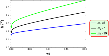
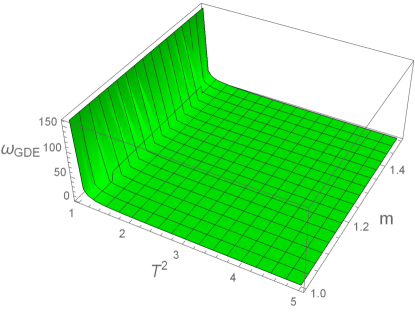
where and , are the integration constants. The right and left panels of Figure 1 show the evolution of against and , respectively for various values of , indicating that the is increasing for both the scenarios as required.
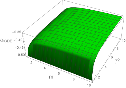
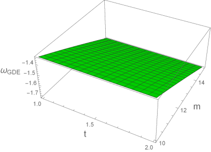
The variation of EoS parameter in the context of gravity is instrumental in delineating the stages of cosmic expansion. For , marking the quintessence era, the universe avoids transitions into either the de Sitter or big rip phases. Quintessence signifies an epoch where cosmic expansion accelerates, albeit at a gradually diminishing rate, attributed to a dynamic form of DE. In contrast, characterizes the phantom epoch, wherein the null energy condition is violated, potentially leading to a catastrophic big rip scenario, with the universe expanding at an increasingly rapid pace. At representing the de Sitter phase, the universe undergoes exponential expansion, mirroring a constant DE density reminiscent of a cosmological constant. In the specific model under scrutiny, within the framework of gravity theory, the observed indicates quintessence era of the universe. This suggests that cosmic expansion is accelerating, yet without the looming prospect of a big rip, aligning with a dynamic DE component akin to quintessence as depicted in the Figure 2. This understanding aids in characterizing the ongoing phase of cosmic evolution and its projected trajectories.

Now, we examine the stability of the reconstructed Garcia-Salcedo GDE model through linear homogeneous perturbations. By analyzing how the model responds to such perturbations, we can assess its viability as a theoretical framework to determine the dynamics of the universe. Furthermore, the stability allows us to identify the conditions under which the model solutions remain consistent and reliable, providing valuable insights to explain observational phenomena such as the accelerated cosmic expansion. In this perspective, we assume [58] and the corresponding energy density becomes
| (27) |
where is the constant energy density. The perturbed energy density and Hubble parameter are given by [58]
| (28) |
We can expand the function as
| (29) |
where indicates that the functions and their derivatives are evaluated in accordance with the solution and term involves the higher power of . Inserting Eqs.(28) and (29) into (9), we have
| (30) |
The second perturbation equation for the conserved energy-momentum tensor is
| (31) |
Using the above two equations, we obtain
| (32) |
Solving this equation, we have
| (33) |
where . Combining Eqs.(30) and (33), we obtain
| (34) |
The stability of the reconstructed Garcia-Salcedo GDE gravity model (26) is obtained by analyzing the associated connections between and as
| (35) | |||||
| (36) | |||||
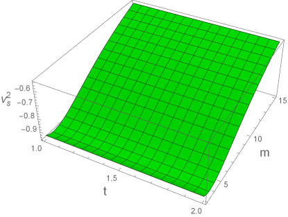
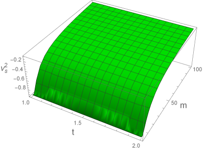
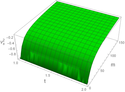
where and . It is observed that the above equations cannot diminish with time in future evolution, consequently, leading to the instability of our model for homogeneous perturbations. Thus the reconstructed Garcia-Salcedo GDE gravity model displays instability which coincides with findings in [55, 58]. We also examine the evolution of the squared sound speed against and in Figure 3, which shows that the corresponding model is unstable as is negative.
3.2 Generalized Ghost Dark Energy Model
The GGDE model is defined through the Veneziano ghost field and the expression for energy density of this model is given by [6]
| (37) |
where and are nonzero constants. The EoS parameter for this model is
| (38) |
Combining the above equation with Eq.(19), we get
| (39) |
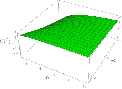
Figure 4 illustrates the function plotted against and . The negative behavior of shows that the functional form is not viable and may lead to matter-dominated era. This is confirmed through the EoS parameter. Inserting Eq.(39) into (19), we obtain the EoS parameter as
| (40) | |||||
The variation of the EoS parameter in Figure 5 indicates that the reconstructed model represents matter-dominated era as , hence is not viable.
4 Reconstruction of Gravity Model
This model stems from the desire to explore novel theoretical frameworks that can effectively describe the cosmic dynamics. This enables us to study the interplay between geometry and matter content in a unified manner, potentially providing deeper insights into cosmological phenomena such as cosmic acceleration and gravitational dynamics on both micro and macro scales. Moreover, this approach offers a significant platform to examine various modifications to GR, which may better align with observational data and address the cosmological puzzles. Inserting this functional form into Eq.(13), we obtain the evolution equation as
| (41) |
To maintain consistency between and the standard continuity equation, the right-hand side of Eq.(13) must be zero. Thus, we obtain
| (42) |
The solution of this equation yields
| (43) |
Here, and are constants and this specific functional form satisfies the standard continuity equation. To reformulate model according to Garcia-Salcedo and GGDE, we assume ( is an arbitrary constant) as [54]
| (44) |
Putting this model in Eq.(41), we have
| (45) |
where
| (46) |
4.1 Garcia-Salcedo GDE Model
First, we explore the Garcia-Salcedo GDE model. Using the GDE model (20), we obtain
| (47) | |||
| (48) |
Putting Eqs.(46)-(48) into (45) yields
| (49) |
Its solution is given as
| (50) | |||||
where , and are constants. The reconstructed Garcia-Salcedo GDE model is obtained by putting the above equation in Eq.(44) as
| (51) | |||||
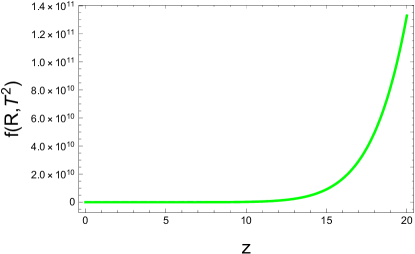
The graphical evolution of the reconstructed Garcia-Salcedo GDE model versus redshift parameter is depicted in Figure 6. We have selected the values of free parameters as , with = 5, 7, 10. The reconstructed model exhibits a gradual increase with the increase in redshift parameter representing the accelerated expansion of the cosmos. Additionally,
| (52) |
which suggests that the reconstructed Garcia-Salcedo GDE model is realistic. The corresponding expressions for energy density and pressure turn out to
| (53) | |||||
| (54) |
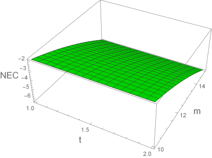
The null energy condition (NEC) plays a crucial role in cosmology, where it serves as a fundamental criterion for the viability of certain DE models. In this context, NEC imposes restrictions on the energy density and pressure of the fluid. Violation of the NEC indicates the exotic matter which leads to unconventional cosmological scenarios such as phantom energy. Understanding and exploring the implications of the violation of NEC is essential for unraveling the mysteries of DE and its role in cosmic acceleration. We study the graphical evolution of the NEC and EoS parameter for Garcia-Salcedo GDE model. The panel on the left hand side of Figure 7 shows that the NEC is violated (, whereas the right panel reveals that the EoS is less than -1, i.e., . Both the conditions favor the cosmic phantom regime. The behavior of squared speed of sound is demonstrated in Figure 8, which shows that the reconstructed Garcia-Salcedo GDE model is unstable.

4.2 Generalized Ghost Dark Energy Model
In this section, we use GGDE model to reconstruct viable model. Using the GGDE model in Eq.(38), we have
| (55) | |||
| (56) |
Inserting Eqs.(46), (55) and (56) into (45), we obtain
| (57) |
The corresponding solution is
| (58) | |||||
The reconstructed GGDE model is obtained as
| (59) | |||||
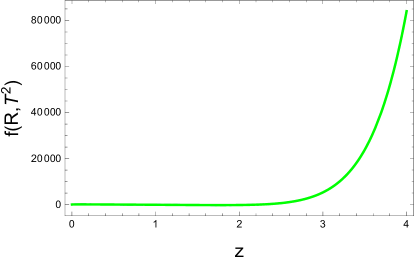
Figure 9 illustrates how the reconstructed GGDE model changes with respect to the redshift parameter for , , , , , and . It is found that the reconstructed model increases gradually with the redshift parameter. Further,
| (60) |
which indicates that the reconstructed model is viable. We examine the behavior of the NEC and EoS parameter for the reconstructed GGDE model against and . Figure 10 indicates that the NEC is violated (left panel) and supports the phantom cosmic era as verified from the EoS parameter (right panel). The stability of the reconstructed GGDE model is checked through the squared speed of sound. Figure 11 shows that the universe dominated by GGDE is not stable.

5 Conclusions
Recent scientific development involves modifying matter by adding a term proportional to . This deviation from linearity has significant consequences for the dynamics of cosmology, especially in the high energy regime. It indicates that interaction with matter itself becomes crucial, particularly in the early stages of the universe. In vacuum, this theory reduces to GR, with its effects primarily affecting the distribution of matter and energy. Researchers are deeply intrigued by the cosmological implications of this modified theory, which goes beyond its relevance in the early universe and rebounding solutions. This has shown its alignment with the solar system test, indicating a broader scope of investigation. This paper studies the reconstruction of the gravity model using the Gracia-Salcedo GDE and GGDE models to discuss the cosmic evolution. The main focus is on the scale factor that represents the phantom era of the universe and leads to a type I singularity [71]. The non-zero conservation of the stress-energy tensor is a key concern in modified theories. To address this issue, the explicit form of the functions and are derived by imposing the constraint of the standard continuity equation.
The Garcia-Salcedo GDE, GGDE models and modified theory each provide unique perspectives and mechanisms that contribute to our understanding of cosmic evolution and expansion. The DE models offer a mechanism for the accelerated expansion of the universe without relying on a cosmological constant. These models explain different phases of cosmic evolution by adjusting the dynamics of ghost fields, leading to transitions between decelerating and accelerating phases of the universe. The GGDE model extends the basic idea of GDE by incorporating additional parameters and functional forms to describe the ghost field’s potential and interactions. By generalizing the ghost field dynamics, these models can produce a richer variety of cosmic evolution scenarios, including different rates of acceleration and transitions between different phases of cosmic expansion. Modified theory encompasses a broad range of models that explain cosmic acceleration. Thus, Garcia-Salcedo GDE, GGDE models and modified gravitational theory provide innovative frameworks that extend beyond the standard cosmological model. They offer new ways to understand the accelerated expansion of the universe and its cosmic evolution, each bringing unique mechanisms and theoretical insights that help to address some of the deepest questions in cosmology.
Here, we provide a summary of our findings for the two models.
-
•
The corresponding to the Garcia-Salcedo GDE (26) (Figure 1) demonstrates increasing behavior which favors the accelerated cosmic expansion and hence is in line with observational data. The EoS parameter is greater than -1, representing quintessence cosmic era (Figure 2) and is consistent with WMAP9 observations [73]. We have also checked the stability against linear homogeneous perturbations, which reveals instability (Figure 3). The reconstructed GGDE model indicates the decreasing behavior, strongly suggesting that this functional form is not viable. The EoS parameter (39) represents the matter dominated era (Figure 5), hence this model lacks viability in the light of recent observational data.
-
•
Here, the gravity Garcia-Salcedo GDE
model shows monotonically increasing behavior as required (Figure
6). The graphical behavior of NEC and the EoS parameter
shows the cosmic phantom regime (Figure 7). Hence, the
Garcia-Salcedo GDE gravity model
supports the cosmic expansion. For the GGDE, the reconstructed model
indicates the fluctuations for both the NEC and the EoS parameter
(Figure 11). Our findings align with the recent
observational data [73].
Data Availability: No data was used for the research
described in this paper.
References
- [1] Witten, E.: Nucl. Phys. B 156(1979)269.
- [2] Veneziano, G.: Nucl. Phys. B 159(1979)213.
- [3] Rosenzweig, C., Schechter, J. and Trahern, C.G.: Phys. Rev. D 21(1980)3388.
- [4] Kawarabayashi, K. and Ohta, N.: Nucl. Phys. B 175(1980)477.
- [5] Nath, P. and Arnowitt, R.L.: Phys. Rev. D 23(1981)473.
- [6] Zhitnitsky, A. R.: Phys. Rev. D 86(2012)045026.
- [7] Ellis, G. F. R.: Comm. Astrophys. 8(1978)7.
- [8] Earman, J. and Eisenstaedt, J.: Stud. Hist. Philos. Sci. B: Stud. Hist. Philos. Mod. Phys. 30(1999)185.
- [9] Nojiri, S. and Odinstov, S.D.: Phys. Rev. D 68(2003)123512.
- [10] Dolgov, A.D. and Kawasaki, M.: Phys. Lett. B 573(2003)4.
- [11] Capozziello, S., Cardone, V.F. and Troisi, A.: Phys. Rev. D 71(2005)043503.
- [12] Capozziello, S. et al.: Phys. Rev. D 73(2006)043512.
- [13] Harko, T. et al.: Phys. Rev. D 84(2011)024020.
- [14] Haghani, Z. et al.: Phys. Rev. D 88(2013)044023.
- [15] Yousaf, Z., Bhatti, M.Z. and Naseer, T.: Phys. Dark Universe 28(2020)100535.
- [16] Yousaf, Z., Bhatti, M.Z., Naseer, T. and Ahmad, I.: Phys. Dark Universe 29(2020)100581.
- [17] Yousaf, Z., Bhatti, M.Z. and Naseer, T.: Eur. Phys. J. Plus 135(2020)323.
- [18] Yousaf, Z., Bhatti, M.Z. and Naseer, T.: Ann. Phys. 420(2020)168267.
- [19] Yousaf, Z., Khlopov, M.Y., Bhatti, M.Z. and Naseer, T.: Mon. Not. R. Astron. Soc. 495(2020)4334.
- [20] Yousaf, Z., Bhatti, M.Z. and Naseer, T.: Int. J. Mod. Phys. D 29(2020)2050061.
- [21] Sardar, G., Bose, A. and Chakraborty, S.: Eur. Phys. J. C 83(2023)41.
- [22] Pradhan, A., Goswami, G. and Beesham, A. Int. J. Geom. Methods Mod. Phys. 20(2023)2350169.
- [23] Malik, A., Asghar, Z. and Shamir, M.F.: New Astron. 104(2023)102071.
- [24] Gul, M.Z. et al.: Eur. Phys. J. C 84(2024)8.
- [25] Rani, S. et al.: Int. J. Geom. Methods Mod. Phys. 21(2024)2450033.
- [26] Blagojevic, M. and Nester, J.M.: Phys. Rev. D 109(2024)064034.
- [27] Gul, M.Z., Sharif, M. and Arooj, A.: Gen. Relativ. Gravit. 56(2024)45.
- [28] Gul, M.Z., Sharif, M. and Arooj, A.: Phys. Scr. 99(2024)045006.
- [29] Gul, M.Z., Sharif, M. and Arooj, A.: Fortschr. Phys. 72(2024)2300221.
- [30] Katirci, N. and Kavuk, M.: Eur. Phys. J. Plus 129(2014)163.
- [31] Roshan, M. and Shojai, F.: Phys. Rev. D 94(2016)044002.
- [32] Board, C.V.R. and Barrow, J.D.: Phys. Rev. D 96(2017)123517.
- [33] Moraes, P.H.R.S. and Sahoo, P.K.: Phys. Rev. D 97(2018)024007.
- [34] Nari, N. and Roshan, M.: Phys. Rev. D 98(2018)024031.
- [35] Barbar, A.H., Awad, A.M., and Al-Fiky, M.T.: Phys. Rev. D 101(2020)044058.
- [36] Sharif, M. and Gul, M.Z.: Phys. Scr. 96(2021)025002; Pramana-J. Phys. 96(2022)153; Chin. J. Phys. 71(2021)35.
- [37] Sharif, M. and Gul, M.Z.: Eur. Phys. J. Plus 136(2021)503; Mod. Phys. Lett. A 36(2021)2150214; Phys. Scr. 96(2021)125007.
- [38] Sharif, M. and Gul, M.Z.: Phys. Scr. 96(2021)105001; Int. J. Mod. Phys. A 36(2021)2150004.
- [39] Sharif, M. and Gul, M.Z.: Chin. J. Phys. 80(2022)58; Int. J. Geom. Methods Mod. Phys. 19(2022)2250012; Mod. Phys. Lett. A 19(2022)2250005.
- [40] Sharif, M. and Gul, M.Z.: Universe 9(2023)145.
- [41] Sharif, M. and Gul, M.Z.: Gen. Relativ. Gravit. 55(2023)10.
- [42] Sharif, M. and Gul, M.Z.: Phys. Scr. 98(2023)035030.
- [43] Sharif, M. and Gul, M.Z.: Fortschr. Phys. 71(2023)2200184.
- [44] Gul, M.Z., Sharif, M.: Symmetry 15(2023)684.
- [45] Sharif, M. and Naz, S.: Ann. Phys. 451(2023)169240.
- [46] Gul, M.Z., Sharif, M. and Afzal, A.: Chin. J. Phys. 89(2024)1347.
- [47] Naseer, T. Sharif, M., Manzoor, S. and Fatima, A.: Mod. Phys. Lett. A 39(2024)2450048.
- [48] Copeland, E.J., Sami, M. and Tujikawa, S.: Int. J. Mod. Phys. D 15(2006)1753.
- [49] Amendola, L., Gannouji, R., Polarski, D. and Tsujikawa, S.: Phys. Rev. D 75(2007)083504.
- [50] Sheykhi, A. and Movahed, M.S.: Gen. Relativ. Gravit. 44(2012)449.
- [51] Odintsov, S.D., Oikonomou, V.K. and Banerjee, S.: Nucl. Phys. B 938(2019)935.
- [52] Chaudhary, H. et al.: Eur. Phys. J. C 83(2023)918.
- [53] Akarsu, O., Nazari, E. and Roshan, M.: Mon. Not. R. Astron. Soc. 523(2023)5452.
- [54] Sharif, M., Gul, M.Z. and Hashim, I.: Chin. J. Phys. 89(2024)266.
- [55] Cai, R.G., Tuo, Z.L., Wu, Y.B. and Zhao, Y.Y.: Phys. Rev. D 86(2012)023511.
- [56] Sheykhi, A., Ebrahimi, E. and Yousefi, Y.: Can. J. Phys. 91(2013)662.
- [57] Karami, K. et al.: Int. J. Mod. Phys. D 22(2013)1350018.
- [58] Zubair, M. and Abbas, G.: Astrophys. Space Sci. 357(2015)154.
- [59] Sharif, M. and Naseer, T.: Gen. Relativ. Gravit. 55(2023)87.
- [60] Naseer, T. and Sharif, M.: Fortschr. Phys. 71(2023)2300004.
- [61] Naseer, T. et al.: Chin. J. Phys. 86(2023)350.
- [62] Sharif, M. and Naseer, T.: Class. Quantum Grav. 40(2023)035009.
- [63] Naseer, T. and Sharif, M.: Chin. J. Phys. 88(2024)10.
- [64] Naseer, T. and Sharif, M.: Fortschr. Phys. 72(2024)2300254.
- [65] Naseer, T. and Sharif, M.: Phys. Scr. 99(2024)035001.
- [66] Sharif, M. and Ajmal, M.: Chin. J. Phys. 88(2024)706.
- [67] Faraoni, V.: Phys. Rev. D 80(2009)124040.
- [68] Feng, C.J., Li, X.Z. and Shen, X.Y.: Mod. Phys. Lett. A 27(2012)1250182.
- [69] Garcia-Salcedo, R. et al.: Phys. Rev. D 88(2013)043008.
- [70] Bertolami, O. et al.: Phys. Rev. D 75(2007)104016.
- [71] Nojiri, S. I. and Odintsov, S. D.: Phys. Rev. D 78(2008)046006.
- [72] Bamba, K., Odintsov, S.D., Sebastiani, L. and Zerbini, S.: Eur. Phys. J. C 67(2010)295.
- [73] Hinshaw, G. et al.: Astrophys. J. Suppl. Ser. 208(2013)19.