Structure-aware Semantic Node Identifiers for Learning on Graphs

Abstract

We present a novel graph tokenization framework that generates structure-aware, semantic node identifiers (IDs) in the form of a short sequence of discrete codes, serving as symbolic representations of nodes. We employs vector quantization to compress continuous node embeddings from multiple layers of a graph neural network (GNN), into compact, meaningful codes, under both self-supervised and supervised learning paradigms. The resulting node IDs capture a high-level abstraction of graph data, enhancing the efficiency and interpretability of GNNs. Through extensive experiments on 34 datasets, including node classification, graph classification, link prediction, and attributed graph clustering tasks, we demonstrate that our generated node IDs not only improve computational efficiency but also achieve competitive performance compared to current state-of-the-art methods. Our implementation is available at https://github.com/LUOyk1999/NodeID.

1 Introduction

Machine learning on graphs involves learning from graph topology and node/edge attributes for tasks such as node/graph classification [44, 18], link prediction [62, 126], community detection [22, 23], and recommendation [46, 20]. Various methods have been developed to address these challenges, including random walk based models [109, 79, 28], spectral methods [4, 13], and graph neural networks (GNNs) [30, 44, 99, 114, 74, 51, 10, 120, 25, 12, 10]. GNNs use a message-passing mechanism [26] to iteratively aggregate information from a node’s neighbors to learn node representations, effectively integrating graph topology and node attributes and achieving impressive results in various tasks.

Despite the advancements in GNNs, their application to large-scale scenarios that require low latency and fast inference remains challenging [124, 38, 117]. The inherent bottleneck lies in the message-passing mechanism of GNNs, which necessitates loading the entire graph—potentially comprising billions of edges—during inference for target nodes, which is both time-consuming and computationally demanding. To address the challenges, recent studies have explored knowledge distillation techniques to distill a small MLP model that captures the essential information from a pre-trained GNN for latency-critical applications [95]. To facilitate the transfer of structural knowledge from GNNs to MLPs, a recent work VQGraph [117] proposes to tokenize nodes using a sizable codebook, with a capacity comparable to the size of the input graph, and use soft code assignment as a target for distillation. Nonetheless, the VQGraph tokenizer is designed to aid the distillation process and lacks the ability to generate sematic codes as meaningful node representations. Moreover, it requires supervised training using class labels, similar to other distillation methods [127, 96].

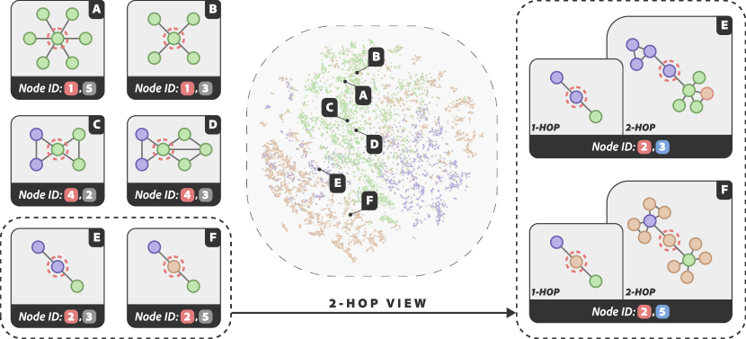
Figure 1: Illustration of structure-aware semantic node IDs generated by our NID framework using a two-layer GCN, with the first ID code derived from the node embedding in the first layer, and the second ID code derived from the node embeddings in the second layer. Center: t-SNE visualization of node embeddings in the PubMed Dataset, with colors representing different class labels. Left: Display of six nodes, each with their ID and 1-hop substructure. Nodes with the same first ID code share similar 1-hop structures, though this does not necessarily indicate the same class label. Right: Nodes E and F are further analyzed with their 2-hop substructures. Variations in these structures are reflected by their distinct second ID code (blue) and class label.

Recent research trends have seen a growing interest in utilizing GNNs as graph tokenizers, which are designed to encode the intricate structures of graphs into tokens for various downstream tasks. Such applications include mining molecular motifs [129, 87, 60], generating multimodal outputs in large language models [60], and representing entities in heterogeneous graphs [61, 94]. Nevertheless, the high-dimensional embeddings generated by GNNs present significant challenges in storage and computational efficiency, and are often difficult to interpret, hindering their use in symbolic systems [48] and other tasks that require comprehensible and compact representations [86].

To overcome these challenges, we introduce a graph tokenization framework for creating structure-aware, semantic node identifiers (node IDs). These IDs consist of a few discrete codes (small integers, up to 32 in our experiments) and serve as compact node representations that can be utilized directly for downstream prediction tasks like classification and clustering. Our Node ID (NID) framework employs vector quantization [27] to compress the continuous node embeddings generated at each layer of a GNN into discrete codes, effectively capturing the multi-order neighborhood structures within the graph and enabling a more efficient representation of node features. Fig. 1 illustrates examples of two-dimensional node IDs generated by a two-layer GNN, demonstrating their ability to capture multi-level structural patterns in the graph. In summary, our contributions are as follows:

• We present NID, a novel graph tokenization framework designed to produce compact, structure-informed, and semantically meaningful symbolic representations of nodes, in both self-supervised and supervised paradigms. The generated node IDs act as a high-level abstraction of the graph data, facilitating symbolic compression and significantly improving inference speed.

• Our extensive evaluation, spanning 34 diverse datasets and covering tasks including node/graph classification, link prediction, and attributed graph clustering tasks, demonstrates that utilizing the generated node IDs can achieve competitive performance with state-of-the-art methods.

2 Preliminaries

We define a graph as a tuple $\mathcal{G}=(\mathcal{V},\mathcal{E},\boldsymbol{X})$, where $\mathcal{V}$ is the set of nodes, $\mathcal{E}\subseteq\mathcal{V}\times\mathcal{V}$ is the set of edges, and $\boldsymbol{X}\in\mathbb{R}^{|\mathcal{V}|\times d}$ is the node feature matrix, with $|\mathcal{V}|$ representing the number of nodes and $d$ the dimension of the node features. Let $\boldsymbol{A}\in\mathbb{R}^{|\mathcal{V}|\times|\mathcal{V}|}$ denote the adjacency matrix of $\mathcal{G}$.

Message Passing Neural Networks (MPNNs) have become the dominant approach for learning graph representations. A typical example is graph convolutional networks (GCNs) [44]. Gilmer et al. [26] reformulated early GNNs into a framework of message passing GNNs, which computes representations $\boldsymbol{h}_{v}^{l}$ for any node $v$ in each layer $l$ as:

$$\boldsymbol{h}_{v}^{l}=\text{UPDATE}^{l}\left(\boldsymbol{h}_{v}^{l-1},\text{AGG}^{l}\left(\left\{\boldsymbol{h}_{u}^{l-1}\mid u\in\mathcal{N}\left(v\right)\right\}\right)\right),$$ (1)

where ${\mathcal{N}}(v)$ denotes the neighborhood of $v$, $\text{AGG}^{l}$ is the message function, and $\text{UPDATE}^{l}$ is the update function. The initial node representation $\boldsymbol{h}_{v}^{0}$ is the node feature vector $\boldsymbol{x}_{v}\in\mathbb{R}^{d}$. The message function aggregates information from the neighbors of $v$ to update its representation. The output of the last layer, i.e., $\text{MPNN}(v,\boldsymbol{A},\boldsymbol{X})=\boldsymbol{h}_{v}^{L}$, is the representation of $v$ produced by the MPNN.

Prediction tasks on graphs involve node-level, edge-level, and graph-level tasks. Each type of tasks requires a tailored graph readout function, $\mathrm{R}$, which aggregates the output node representations, $\boldsymbol{h}_{v}^{L}$, from the last layer $L$, to compute the final prediction result:

$$\boldsymbol{h}_{\text{readout}}=\mathrm{R}\left(\left\{\boldsymbol{h}_{v}^{L},v\in\mathcal{V}\right\}\right).$$ (2)

Specifically, for node-level tasks, which involve classifying individual nodes, $\mathrm{R}$ is simply an identity mapping. For edge-level tasks, which focus on analyzing the relationship between any node pair $(u,v)$, $\mathrm{R}$ is typically modeled as the Hadamard product of the node representations [43], i.e., $\boldsymbol{h}_{\text{readout}}=\boldsymbol{h}_{v}^{L}\odot\boldsymbol{h}_{u}^{L}$. For graph-level tasks that aim to make predictions about the entire graph, $\mathrm{R}$ often functions as a global mean pooling operation, expressed as $\boldsymbol{h}_{\text{readout}}=\frac{1}{|\mathcal{V}|}\sum_{v\in\mathcal{V}}\boldsymbol{h}_{v}^{L}$.

Vector Quantization (VQ) [27, 68] aims to represent a large set of vectors, $\boldsymbol{Z}=\{\boldsymbol{z}_{i}\}_{i=1}^{N}$, with a small set of prototype (code) vectors of a codebook $\boldsymbol{C}=\{\boldsymbol{c}_{j}\}_{j=1}^{K}$, where $N\gg K$. The codebook is often created using algorithms such as $k$-means clustering via optimizing the following objective:

$$\textbf{VQ:}~{}~{}~{}\min_{\boldsymbol{C}}\sum_{i=1}^{N}\min_{j=1}^{K}\left|\left|\boldsymbol{z}_{i}-\boldsymbol{c}_{j}\right|\right|_{2}^{2}.$$ (3)

Once the codebook is learned, each vector $\boldsymbol{z}_{i}$ can be approximated by its closet prototype vector $\boldsymbol{c}_{t}$, where $t=\arg\min_{j}\left|\left|\boldsymbol{z}_{i}-\boldsymbol{c}_{j}\right|\right|_{2}^{2}$ is the index of the prototype vector. Residual Vector Quantization (RVQ) [39, 69] is an extension of the basic VQ. After performing an initial VQ, the residual vector, i.e., the difference between the original vector and the approximation is calculated:

$$\boldsymbol{r}_{i}=\boldsymbol{z}_{i}-\boldsymbol{c}_{t},$$ (4)

which represents the quantization error from the initial quantization. Then, the residual vectors $\boldsymbol{r}_{i}$ are quantized using a second codebook. This process can be repeated multiple times, with each stage quantizing the residual error from the previous stage. In this manner, RVQ can enhance quantization accuracy by iteratively quantizing the residual error.

3 Our Proposed Node ID (NID) Framework

Our proposed NID framework consists of two stages:

1. Generating structure-aware semantic node IDs. We encode nodes by using multi-layer MPNNs to capture multi-order neighborhood structures. At each layer, the node embedding is quantized into a tuple of structural codewords. The tuples are then combined to form what we refer to as the node ID.

2. Utilizing the generated node IDs as compact, informative features in various downstream tasks. We directly use the node IDs for unsupervised tasks like node clustering, and train simple MLPs with the node IDs for supervised tasks including node classification, link prediction, and graph classification.

3.1 Generation of Structure-aware Semantic Node IDs

Fig. 3 shows that the node representations produced by MPNNs at different layer $l$ exhibit diverse clustering patterns, which is due to the cumulative smoothing effect resulting from successive applications of graph convolution at each layer [52, 53]. Hence, to generate structure-aware semantic node IDs, we employ an $L$-layer MPNN to capture multi-order neighborhood structures. At each layer, we use vector quantization to encode the node embeddings produced by the MPNN into $M$ codewords (integer indices). For each node $v$, we define the node ID of $v$ as a tuple composed of $L\times M$ codewords, structured as follows:

$$\text{Node\_ID}(v)=\left(c_{11},\cdots,c_{1M},c_{21},\cdots,c_{2M},\cdots,c_{L1},\cdots,c_{LM}\right),$$ (5)

where $c_{lm}$ represents the $m$-th codeword at the $l$-th layer. Both $M$ and $L$ can be very small. For the node IDs in Fig. 1, $M=1$ and $L=2$. In our experiments, we typically set $M=3$ and $L\in[2,5]$.

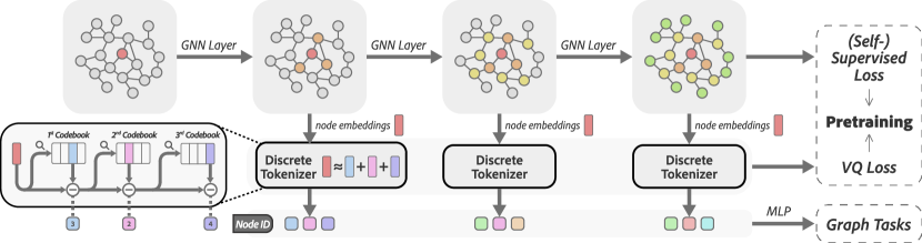
Figure 2: Overview of our proposed framework.

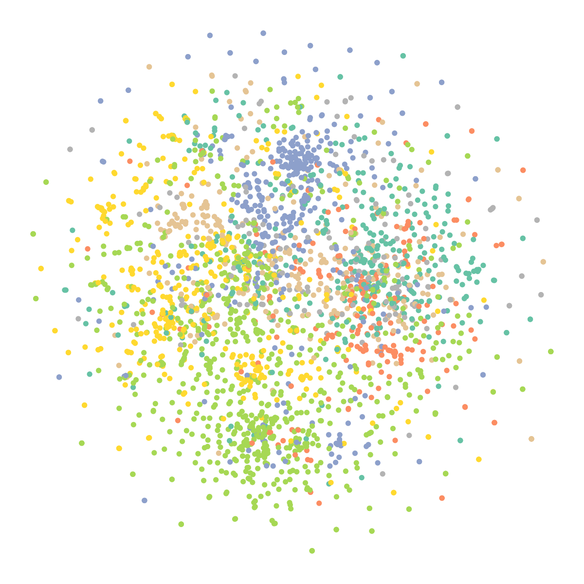
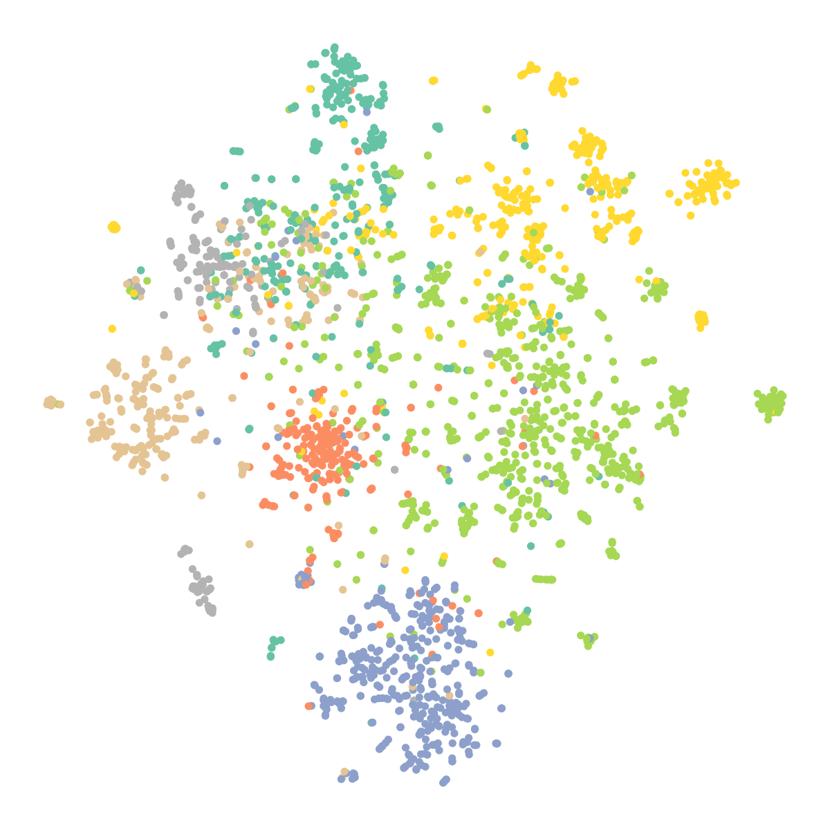
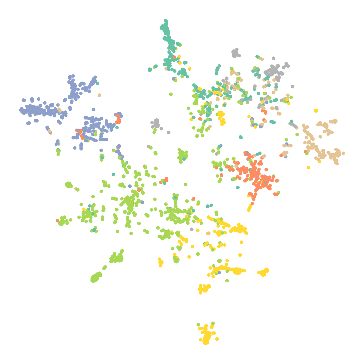
(a) Raw features     (b) $l=1$     (c) $l=3$     

Figure 3: t-SNE visualization of the node representations of the Cora dataset generated by an MPNN at different layer $l$. The node representations exhibit different cluster structures for different $l$.

Learning Node IDs. As illustrated in Fig. 2, at each layer $l$ ($1\leq l\leq L)$ of the MPNN, we employ RVQ (see Sec. 2) to quantize the node embeddings and produce $M$ tiers of codewords for each node $v$. Each codeword $c_{lm}$ ($1\leq m\leq M$) is generated by a distinct codebook $\boldsymbol{C}_{lm}=\{\boldsymbol{e}_{k}\}^{K}_{k=1}$, where $K$ is the size of the codebook. Hence, there are a total of $L\times M$ codebooks. Let $\boldsymbol{r}_{lm}$ denote the (residual) vector to be quantized. When $m=1$, $\boldsymbol{r}_{l1}$ is the node embedding $\boldsymbol{h}_{v}^{l}$ produced by the MPNN. Then, $\boldsymbol{r}_{lm}$ is approximated by its nearest code vector from the corresponding codebook $\boldsymbol{C}_{lm}$:

$$c_{lm}=\arg\min_{k}||\boldsymbol{r}_{lm}-\boldsymbol{e}_{k}||,$$ (6)

producing the codeword $c_{lm}$, which is the index of the nearest code vector.

We introduce a simple, generic framework for learning node IDs (codewords $c_{lm}$) by jointly training the MPNN and the codebooks with the following loss function:

$$\mathcal{L}_{\text{NID}}=\mathcal{L}_{\mathcal{G}}+\mathcal{L}_{\text{VQ}},$$ (7)

where $\mathcal{L}_{\mathcal{G}}$ is a (self)-supervised graph learning objective, and $\mathcal{L}_{\text{VQ}}$ is a vector quantization loss. $\mathcal{L}_{\mathcal{G}}$ aims to train the MPNN to produce structure-aware node embeddings, while $\mathcal{L}_{\text{VQ}}$ ensures the codebook vectors align well with the node embeddings. For a single node $v$, $\mathcal{L}_{\text{VQ}}$ is defined as

$$\mathcal{L}_{\text{VQ}}=\sum_{l=1}^{L}\sum_{m=1}^{M}\|\text{sg}(\boldsymbol{r}_{lm})-\boldsymbol{e}_{c_{lm}}\|+\beta\|\boldsymbol{r}_{lm}-\text{sg}(\boldsymbol{e}_{c_{lm}})\|,$$ (8)

where sg denotes the stop gradient operation, and $\beta$ is a weight parameter. The first term in Eq. (8) is the codebook loss [98], which only affects the codebook and brings the selected code vector close to the node embedding. The second term is the commitment loss [98], which only influences the node embedding and ensures the proximity of the node embedding to the selected code vector. In practice, we can use exponential moving averages [85] as a substitute for the codebook loss.

Self-supervised Learning. The graph learning objective $\mathcal{L}_{\mathcal{G}}$ can be a self-supervised learning task, such as graph reconstruction (i.e., reconstructing the node features or graph structures) or contrastive learning [59]. In this paper, we examine two representative models: GraphMAE [33] and GraphCL [122]. We discuss GraphMAE here and address GraphCL in the App. A due to space limitations. Specifically, GraphMAE involves sampling a subset of nodes $\tilde{\mathcal{V}}\subset\mathcal{V}$, masking the node features as $\tilde{\boldsymbol{X}}$, encoding the masked node features using an MPNN, and subsequently reconstructing the masked features with a decoder. The reconstruction loss is based on the scaled cosine error, expressed as:

$$\mathcal{L}_{\mathcal{G}}=\mathcal{L}_{\text{MAE}}=\frac{1}{|\tilde{\mathcal{V}}|}\sum_{v\in\tilde{\mathcal{V}}}\left(1-\frac{\boldsymbol{x}_{v}^{T}\boldsymbol{z}_{v}}{\|\boldsymbol{x}_{v}\|\cdot\|\boldsymbol{z}_{v}\|}\cdot\gamma\right),$$

where $\tilde{\mathcal{V}}$ is the set of masked nodes, $\boldsymbol{z}_{v}=f_{D}(\tilde{\boldsymbol{h}}_{v}^{L})$ is the reconstructed node features by a decoder $f_{D}$, $\tilde{\boldsymbol{h}}_{v}^{L}=\text{MPNN}(v,\boldsymbol{A},\tilde{\boldsymbol{X}})$, and $\gamma\geq 1$ is a scaling factor. Let $\tilde{\boldsymbol{r}}_{l1}:=\tilde{\boldsymbol{h}}_{v}^{l}$ denote the node embedding generated by the $l$-th layer of the MPNN with the masked features. The overall training loss is

$$\mathcal{L}_{\text{NID}}=\mathcal{L}_{\text{MAE}}+\sum_{v\in\tilde{\mathcal{V}}}\sum_{l=1}^{L}\sum_{m=1}^{M}\|\text{sg}(\tilde{\boldsymbol{r}}_{lm})-\boldsymbol{e}_{c_{lm}}\|+\beta\|\tilde{\boldsymbol{r}}_{lm}-\text{sg}(\boldsymbol{e}_{c_{lm}})\|.$$ (9)

Supervised Learning. The graph learning objective $\mathcal{L}_{\mathcal{G}}$ can also be a supervised learning task, such as node classification, link prediction, or graph classification. For classification tasks, $\mathcal{L}_{\mathcal{G}}$ can be the cross-entropy loss between the target label $y$ and the prediction $\boldsymbol{h}_{\text{readout}}$ (see Eq. (2)) given by the MPNN:

$$\mathcal{L}_{\mathcal{G}}=\mathcal{L}_{\text{CE}}(y,\boldsymbol{h}_{\text{readout}}).$$ (10)

Remark. Our NID framework differs from VQ-VAE [98] and similar approaches [49, 117] in codebook learning. Unlike these methods, our training objective $\mathcal{L}_{\text{NID}}$ does not involve using the code vectors ($\boldsymbol{e}_{k}$) for a reconstruction task. Instead, we guide the codebook learning process solely via graph learning tasks ($\mathcal{L}_{\mathcal{G}}$). Moreover, our NID framework is compatible with any MPNN model. In experiments, we use popular models like GCN [44], GAT [99], GraphSAGE [30] and GIN [114].

3.2 Applications of Node IDs for Graph Learning

The generated structure-aware semantic node IDs can be considered as highly compact node representations and used directly for various downstream graph learning tasks, as outlined below.

Node-level tasks include node classification and node clustering. For node classification, each node $v$ in the graph is associated with a label $y_{v}$, representing its category. We can directly utilize the node IDs of the labeled nodes to train an MLP network for classification. The prediction is formulated as

$$\hat{y}_{v}=\text{MLP}(\text{Node\_ID}(v)).$$ (11)

For node clustering, one can directly apply vector-based clustering algorithms such as $k$-means [67] or mean shift [24] to the node IDs to obtain clustering results.

Edge-level tasks typically involve link prediction. The aim is to predict whether an edge should exist between any node pair $(u,v)$. The prediction can be made by

$$\hat{y}_{(u,v)}=\text{MLP}(\text{Node\_ID}(u)\odot\text{Node\_ID}(v)),$$ (12)

where $\odot$ is the Hadamard product.

Graph-level tasks include graph classification and graph regression. These tasks involve predicting a categorical label or numerical value for the entire graph $\mathcal{G}$. The prediction can be formulated as

$$\hat{y}_{\mathcal{G}}=\text{MLP}(\frac{1}{|\mathcal{V}|}\sum_{v\in\mathcal{V}}\text{Node\_ID}(v)),$$ (13)

where a global mean pooling function is applied on all the node IDs to generate a representation for the graph $\mathcal{G}$, which is then input into an MLP for prediction. Note that the selection of the readout function, such as mean pooling, is considered a hyper-parameter.

Remark. Due to the high compactness of the node IDs, which usually consists of multiple codewords (int4), the training and inference processes of the aforementioned graph learning tasks can be greatly accelerated. Furthermore, as illustrated in Fig. 1, the node IDs represent a high-level abstraction of structural and semantic information in a graph, enabling them to achieve competitive performance across various tasks, as evidenced in our evaluation.

4 Evaluation

In this section, we demonstrate the versatility of our NID framework across various graph learning tasks. We detail its application in two distinct scenarios:

• Unsupervised representation learning for node classification, attributed graph clustering and graph classification. In these unsupervised tasks, NID is benchmarked against well-known contrastive and generative SSL methods. We adhere strictly to the established experimental procedures, including data splits and evaluation protocols, as the standard settings [33, 122, 128].

• Supervised representation learning for node classification, link prediction and graph classification. Here, we evaluate our NID against several SOTA models for graph representation learning, following conventional supervised learning protocols [14, 108, 83, 105].

RVQ Implementation Details. As outlined in Sec. 3.1, RVQ is used to quantize the MPNN multi-layer embeddings of a node. The selection of MPNNs and the number of layers $L$ are tailored to distinct datasets. For the embeddings from each layer, a consistent three-level ($M=3$) residual quantization is implemented. The codebook size $K$ is tuned in $\{4,6,8,16,32\}$. The $\beta$ is set to 1.

Table 1: Node classification results in unsupervised representation learning (%).

	Cora	CiteSeer	PubMed
Metric	Accuracy$\uparrow$	Accuracy$\uparrow$	Accuracy$\uparrow$	dim
GAE	71.5 ± 0.4	65.8 ± 0.4	72.1 ± 0.5	16
DGI	82.3 ± 0.6	71.8 ± 0.7	76.8 ± 0.6	512
MVGRL	83.5 ± 0.4 (3)	73.3 ± 0.5	80.1 ± 0.7 (3)	512
InfoGCL	83.5 ± 0.3 (3)	73.5 ± 0.4 (2)	79.1 ± 0.2	512
CCA-SSG	84.0 ± 0.4 (2)	73.1 ± 0.3	81.0 ± 0.4 (2)	512
MLP	57.8 ± 0.5	54.7 ± 0.4	73.3 ± 0.6	500
GraphMAE	84.2 ± 0.4 (1)	73.4 ± 0.4 (3)	81.1 ± 0.4 (1)	512
$\textbf{NID}_{\text{MAE}}$	80.8 ± 0.7	74.2 ± 0.6 (1)	76.4 ± 0.8	6

Table 2: Attributed graph clustering results; Clustering accuracy, normalized mutual information, and macro-F1 (%).

		Cora			CiteSeer
Metric	Acc$\uparrow$	NMI$\uparrow$	F1$\uparrow$	Acc$\uparrow$	NMI$\uparrow$	F1$\uparrow$	dim
DeepWalk	46.74	31.75	38.06	36.15	9.66	26.70	128
GAE	53.25	40.69	41.97	41.26	18.34	29.13	16
MGAE	63.43	45.57	38.01	63.56	39.75	39.49	16
ARGE	64.00	44.90	61.90	57.30	35.00	54.60	16
AGC	68.92	53.68	65.61	67.00	41.13	62.48	500
$k$-means	34.65	16.73	25.42	57.32	29.12	57.35	500
GraphMAE	66.94	51.89	64.24	68.78	43.78	64.27	512
$\textbf{NID}_{\text{MAE}}$	74.51	56.92	69.80	71.35	44.98	66.16	6

Table 3: Graph classification results in unsupervised representation learning on TUDataset; Accuracy (%).

Methods	NCI1	PROTEINS	DD	MUTAG	COLLAB	RDT-B	RDT-M5K	IMDB-B
# graphs	4,110	1,113	1,178	188	5,000	2,000	4,999	1,000
Avg. # nodes	29.8	39.1	284.3	17.9	74.5	429.7	508.5	19.8
graph2vec	73.2 ± 1.8	73.3 ± 2.0	70.3 ± 2.3	83.1 ± 9.2	71.1 ± 0.5 (3)	75.7 ± 1.0	47.8 ± 0.2	71.1 ± 0.5 (3)
InfoGraph	76.2 ± 1.0 (3)	74.4 ± 0.3 (2)	72.8 ± 1.7	89.0 ± 1.1 (1)	70.6 ± 1.1	82.5 ± 1.4	53.4 ± 1.0	73.0 ± 0.8 (1)
JOAO	78.3 ± 0.5 (1)	74.0 ± 1.1	77.4 ± 1.1 (3)	87.6 ± 0.7 (3)	69.3 ± 0.3	86.4 ± 1.4 (3)	56.0 ± 0.2 (1)	70.8 ± 0.2
GraphCL	77.8 ± 0.4 (2)	74.3 ± 0.4 (3)	78.6 ± 0.4 (1)	86.8 ± 1.3	71.3 ± 1.1 (2)	89.5 ± 0.8 (2)	55.9 ± 0.2 (2)	71.1 ± 0.4 (3)
$\textbf{NID}_{\text{CL}}$	75.9 ± 0.6	75.1 ± 0.5 (1)	77.8 ± 1.1 (2)	88.6 ± 1.7 (2)	76.9 ± 0.3 (1)	90.7 ± 0.9 (1)	55.0 ± 0.5 (3)	72.3 ± 1.2 (2)

Detailed datasets, baselines, and hyperparameters are provided in Appendix B due to space constraints.

4.1 Self-supervised Node IDs for Unsupervised Representation Learning

Node Classification, Table 2. We evaluate the performance of our NID on three standard benchmarks: Cora, CiteSeer, and PubMed [118]. For this purpose, we employ GraphMAE to provide graph learning objective during the training of node IDs. Specifically, we train a 2-layer GAT following the GraphMAE without supervision, resulting in the generation of 6-dim node IDs, denoted as $\textbf{NID}_{\text{MAE}}$. Subsequently, we train an MLP and report the mean accuracy on the test nodes. For the evaluation protocol, we follow all the experimental settings used in GraphMAE [33], including data splits and evaluation metrics, using all baselines reported by [33]. Table 2 lists the results. MLP refers to predictions made directly on the initial node features. Notably, $\textbf{NID}_{\text{MAE}}$ achieves competitive results in comparison to SOTA self-supervised approaches, and even surpasses all other approaches on CiteSeer. Remarkably, our node IDs are comprised of only 6 discrete codes, with each code having a maximum of 32 possible values. This demonstrates that our NID framework effectively compresses the node’s structure-aware semantic information into a concise yet information-rich representation.

Attributed Graph Clustering, Table 2. Attributed graph clustering [5] aims to cluster nodes of an attributed graph, where each node is associated with a set of feature attributes. In this study, we select the Cora and CiteSeer datasets, in which the nodes are associated with binary word vectors. We apply the $k$-means algorithm directly to the $\textbf{NID}_{\text{MAE}}$ codes to derive clustering results. We utilize all the clustering performance measures and baselines from AGC [128] for comparison. We report the clustering results in Table 2. $\textbf{NID}_{\text{MAE}}$ outperforms all baseline models by a considerable margin on the Cora, CiteSeer, and PubMed. Notably, due to the short dimensionality of our node IDs, the $k$-means clustering operates significantly faster with our representation compared to other embeddings. We plan to investigate this advantage further in very large networks in our future work.

Graph Classification, Tables 3 and 14. We evaluate our NID framework on 8 datasets from TUDataset [73]: NCI1, PROTEINS, DD, MUTAG, COLLAB, REDDIT-B, REDDIT-M5K, and IMDB-B, utilizing GraphCL as graph learning objective to guide node ID pre-training due to its superior performance in graph classification. Specifically, we employ a GIN with the default settings from GraphCL as the GNN-based encoder, denoted as $\textbf{NID}_{\text{CL}}$. For the evaluation protocol, we input node IDs into a downstream LIBSVM [8] classifier, reporting the mean 10-fold cross-validation accuracy with standard deviation after five runs. All baselines are taken from GraphCL [122]. The results are presented in Table 3, where $\textbf{NID}_{\text{MAE}}$ outperforms all baselines on 3 out of 8 datasets. This performance demonstrate that our NID framework is capable of learning meaningful information and demonstrates significant potential for application in graph-level tasks. Additional linear probing results on 7 MoleculeNet datasets [110] are discussed in Appendix C, showing consistent findings.

Table 4: Node classification results in supervised representation learning over homophilic graphs (%). The baseline results are primarily taken from [14], with the remaining obtained from their respective original papers.

	Cora	CiteSeer	PubMed	Computer	Photo	CS	Physics	WikiCS
# nodes	2,708	3,327	19,717	13,752	7,650	18,333	34,493	11,701
# edges	5,278	4,732	44,324	245,861	119,081	81,894	247,962	216,123
Metric	Accuracy$\uparrow$	Accuracy$\uparrow$	Accuracy$\uparrow$	Accuracy$\uparrow$	Accuracy$\uparrow$	Accuracy$\uparrow$	Accuracy$\uparrow$	Accuracy$\uparrow$
MLP	75.69 ± 2.00	72.41 ± 2.18	86.65 ± 0.35	84.51 ± 0.41	91.63 ± 0.26	94.49 ± 0.08	96.01 ± 0.28	72.34 ± 0.19
GCN	86.98 ± 1.27	76.50 ± 1.36	88.42 ± 0.50	89.65 ± 0.52	92.70 ± 0.20	92.92 ± 0.12	96.18 ± 0.07	77.47 ± 0.85
SAGE	86.05 ± 1.87	75.58 ± 1.33	87.48 ± 0.38	91.20 ± 0.29	94.59 ± 0.14	93.91 ± 0.13	96.49 ± 0.06	74.77 ± 0.95
GAT	87.30 ± 1.10	76.55 ± 1.23	86.33 ± 0.48	90.78 ± 0.13	93.87 ± 0.11	93.61 ± 0.14	96.17 ± 0.08	76.91 ± 0.82
GCNII	88.37 ± 1.25 (3)	77.33 ± 1.48 (3)	90.15 ± 0.43 (2)	91.04 ± 0.41	94.30 ± 0.20	92.22 ± 0.14	95.97 ± 0.11	78.68 ± 0.55 (4)
GPRGNN	87.95 ± 1.18	77.13 ± 1.67 (4)	87.54 ± 0.38	89.32 ± 0.29	94.49 ± 0.14	95.13 ± 0.09 (4)	96.85 ± 0.08	78.12 ± 0.23
APPNP	87.87 ± 0.82	76.53 ± 1.16	88.43 ± 0.15	90.18 ± 0.17	94.32 ± 0.14	94.49 ± 0.07	96.54 ± 0.07	78.87 ± 0.11 (3)
tGNN	88.08 ± 1.31	77.51 ± 1.92 (1)	90.80 ± 0.18 (1)	83.40 ± 1.33	89.92 ± 0.72	92.85 ± 0.48	96.24 ± 0.24	71.49 ± 1.05
GraphGPS	87.64 ± 0.97	76.99 ± 1.12	88.94 ± 0.16	91.19 ± 0.54	95.06 ± 0.13	93.93 ± 0.12	97.12 ± 0.19 (4)	78.66 ± 0.49 (5)
NAGphormer	88.15 ± 1.28 (4)	77.42 ± 1.41 (2)	89.70 ± 0.19 (3)	91.22 ± 0.14 (5)	95.49 ± 0.11 (3)	95.75 ± 0.09 (1)	97.34 ± 0.03 (1)	77.16 ± 0.72
Exphormer	88.64 ± 1.65 (2)	76.83 ± 1.24	89.67 ± 0.26 (4)	91.47 ± 0.17 (4)	95.35 ± 0.22 (4)	94.93 ± 0.01 (5)	96.89 ± 0.09 (5)	78.54 ± 0.49
GOAT	87.86 ± 1.31	76.89 ± 1.19 (5)	86.87 ± 0.24	90.96 ± 0.90	92.96 ± 1.48	94.21 ± 0.38	96.24 ± 0.24	77.00 ± 0.77
NodeFormer	88.80 ± 0.26 (1)	76.33 ± 0.59	89.32 ± 0.25	86.98 ± 0.62	93.46 ± 0.35	95.64 ± 0.22 (2)	96.45 ± 0.28	74.73 ± 0.94
DIFFormer	87.63 ± 0.81	76.72 ± 0.68	89.51 ± 0.67 (5)	91.99 ± 0.76 (3)	95.10 ± 0.47 (5)	94.78 ± 0.20	96.60 ± 0.18	73.46 ± 0.56
Polynormer	88.11 ± 1.08 (5)	76.77 ± 1.01	87.34 ± 0.43	93.18 ± 0.18 (2)	96.11 ± 0.23 (2)	95.51 ± 0.29 (3)	97.22 ± 0.06 (2)	79.53 ± 0.83 (2)
NID	87.88 ± 0.69	76.89 ± 1.09 (5)	89.42 ± 0.44	93.38 ± 0.16 (1)	96.47 ± 0.27 (1)	94.75 ± 0.16	97.13 ± 0.08 (3)	79.56 ± 0.43 (1)

Table 5: Node classification results in supervised learning on heterophilic graphs (%).

	Squirrel	Chameleon	Amazon-R
# nodes	2223	890	24,492
# edges	46,998	8,854	93,050
Metric	Accuracy$\uparrow$	Accuracy$\uparrow$	Accuracy$\uparrow$
MLP	35.83 ± 0.95	28.74 ± 2.83	49.84 ± 0.17
GCN	38.67 ± 1.84	41.31 ± 3.05	48.70 ± 0.63
SAGE	36.09 ± 1.99	37.77 ± 4.14	53.63 ± 0.39
GAT	35.62 ± 2.06	39.21 ± 3.08	52.70 ± 0.62
H2GCN	35.10 ± 1.15	26.75 ± 3.64	36.47 ± 0.23
GPRGNN	38.95 ± 1.99	39.93 ± 3.30	44.88 ± 0.34
FSGNN	35.92 ± 1.32	40.61 ± 2.97	52.74 ± 0.83
GloGNN	35.11 ± 1.24	25.90 ± 3.58	36.89 ± 0.14
GraphGPS	39.67 ± 2.84	40.79 ± 4.03	53.10 ± 0.42
NodeFormer	38.52 ± 1.57	34.73 ± 4.14	43.86 ± 0.35
SGFormer	41.80 ± 2.27	44.93 ± 3.91	48.01 ± 0.49
Polynormer	40.87 ± 1.96	41.82 ± 3.45	54.46 ± 0.40
NID	45.09 ± 1.72	46.29 ± 2.92	54.92 ± 0.42

Table 6: Node classification results in supervised representation learning on large-scale graphs (%).

	ogbn-proteins	ogbn-arxiv	ogbn-products	pokec
# nodes	132,534	169,343	2,449,029	1,632,803
# edges	39,561,252	1,166,243	61,859,140	30,622,564
Metric	ROC-AUC$\uparrow$	Accuracy$\uparrow$	Accuracy$\uparrow$	Accuracy$\uparrow$
MLP	72.04 ± 0.48	55.50 ± 0.23	61.06 ± 0.08	62.24 ± 0.23
GCN	72.51 ± 0.35	71.74 ± 0.29	75.64 ± 0.21	75.45 ± 0.17
GAT	72.02 ± 0.44	71.95 ± 0.36 (4)	79.45 ± 0.59 (5)	72.23 ± 0.18
GPRGNN	75.68 ± 0.49 (5)	71.10 ± 0.12	79.76 ± 0.59 (4)	78.83 ± 0.05 (4)
LINKX	71.37 ± 0.58	66.18 ± 0.33	71.59 ± 0.71	82.04 ± 0.07 (3)
GraphGPS	76.83 ± 0.26 (3)	70.97 ± 0.41	OOM	OOM
GOAT	74.18 ± 0.37	72.41 ± 0.40 (3)	82.00 ± 0.43 (2)	66.37 ± 0.94
NodeFormer	77.45 ± 1.15 (2)	59.90 ± 0.42	72.93 ± 0.13	71.00 ± 1.30
SGFormer	79.53 ± 0.38 (1)	72.63 ± 0.13 (1)	74.16 ± 0.31	73.76 ± 0.24
NAGphormer	73.61 ± 0.33	70.13 ± 0.55	73.55 ± 0.21	76.59 ± 0.25 (5)
Exphormer	74.58 ± 0.26	72.44 ± 0.28 (2)	OOM	OOM
Polynormer	74.97 ± 0.47	71.82 ± 0.23 (5)	82.97 ± 0.28 (1)	85.95 ± 0.07 (1)
NID	76.78 ± 0.59 (4)	71.27 ± 0.24	81.83 ± 0.26 (3)	85.63 ± 0.31 (2)

4.2 Supervised Node IDs for Supervised Representation Learning

Node Classification, Tables 4, 6, 6, Figure 6. We have conducted extensive evaluations on 8 homophilic and 3 heterophilic graphs, and tested scalability on 4 large-scale graphs, each with millions of nodes. We compare NID against 11 competitive GNNs and 8 Graph Transformers (GTs), all of which have shown promising results in node classification tasks. All experimental settings are maintained as described by [14, 108]. As demonstrated in Table 4, our NID is competitive with the SOTA method, Polynormer, over homophilic graphs. Table 6 reports the results on heterophilic graphs. Notably, NID surpasses all baselines across these three datasets, highlighting its superior global information capture, a key advantage for heterophilic graphs [54]. This is attributed to the VQ process, which involves joint learning across all nodes, thereby introducing a novel method of incorporating global information into graph domains, distinctly different from the GTs.

As shown in Table 6, our NID also achieves near-SOTA performance on datasets with millions of nodes. Notably, our IDs require only a small fraction of labels for training. For instance, in the case of the ogbn-products dataset, only 8% of the data is used for training. We analyze the training ratio in Figure 6, showing that merely 10% of the training dataset is sufficient to train node IDs that achieve effective predictive performance. Compared to unsupervised scenarios, supervised NID shows superior results relative to the baselines, likely due to the VQ process effectively capturing coherent clustering structures created by MPNN embeddings during supervised learning.

Link Prediction, Table 8. We test our NID on 5 well-known benchmarks for link prediction: Cora, Citeseer, Pubmed and two from the Open Graph Benchmark (OGB)—ogbl-collab and ogbl-ppa [34]. We adhere to the data splits, evaluation metrics and baselines specified by the NCN [105]. The experimental results are presented in Table 8. NID also exhibits competitive capabilities in link prediction tasks. These impressive results underscore the outstanding versatility of our framework.

Graph Classification, Table 8. We test on two peptide graph benchmarks from the LongRange Graph Benchmark (LRGB) [19]: Peptides-func and Peptides-struct. We take all evaluation protocols suggested by [83]. We compare NID against SOTA GNNs and GTs designed for graph-level tasks. As evidenced in Table 8, simply applying pooling to the node IDs result in excellent performance. This underscores the significant potential of our NID for supervised learning in graph-level tasks.

Table 7: Graph-level performance in supervised representation learning from LRGB.

	Peptides-func	Peptides-struct
Avg. # nodes	150.9	150.9
Avg. # edges	307.3	307.3
Metric	AP$\uparrow$	MAE$\downarrow$
GCN	0.5930 ± 0.0023	0.3496 ± 0.0013
GatedGCN	0.5864 ± 0.0035	0.3420 ± 0.0013
GT	0.6326 ± 0.0126	0.2529 ± 0.0016
GraphGPS	0.6535 ± 0.0041	0.2500 ± 0.0012
GRIT	0.6988 ± 0.0082 (1)	0.2460 ± 0.0012 (2)
Exphormer	0.6527 ± 0.0043	0.2481 ± 0.0007 (3)
Graph ViT	0.6970 ± 0.0080 (2)	0.2449 ± 0.0016 (1)
NID	0.6608 ± 0.0058 (3)	0.2589 ± 0.0014

Table 8: Edge-level performance in supervised representation learning. The link prediction baselines are taken from NCN [105] (%).

	Cora	CiteSeer	PubMed	ogbl-collab	ogbl-ppa
# nodes	2,708	3,327	19,717	235,868	576,289
# edges	5,278	4,552	44,324	1,285,465	30,326,273
Metric	HR@100$\uparrow$	HR@100$\uparrow$	HR@100$\uparrow$	HR@50$\uparrow$	HR@100$\uparrow$
GCN	66.79 ± 1.65	67.08 ± 2.94	53.02 ± 1.39	44.75 ± 1.07	18.67 ± 1.32
SAGE	55.02 ± 4.03	57.01 ± 3.74	39.66 ± 0.72	48.10 ± 0.81	16.55 ± 2.40
SEAL	81.71 ± 1.30	83.89 ± 2.15	75.54 ± 1.32 (3)	64.74 ± 0.43 (3)	48.80 ± 3.16
NBFnet	71.65 ± 2.27	74.07 ± 1.75	58.73 ± 1.99	OOM	OOM
Neo-GNN	80.42 ± 1.31	84.67 ± 2.16	73.93 ± 1.19	57.52 ± 0.37	49.13 ± 0.60
BUDDY	88.00 ± 0.44 (3)	92.93 ± 0.27 (1)	74.10 ± 0.78	65.94 ± 0.58 (1)	49.85 ± 0.20 (3)
NCN	89.05 ± 0.96 (2)	91.56 ± 1.43 (2)	79.05 ± 1.16 (1)	64.76 ± 0.87 (2)	61.19 ± 0.85 (1)
NID	90.33 ± 0.76 (1)	88.56 ± 0.72 (3)	75.67 ± 0.63 (2)	64.31 ± 0.48	52.37 ± 0.54 (2)

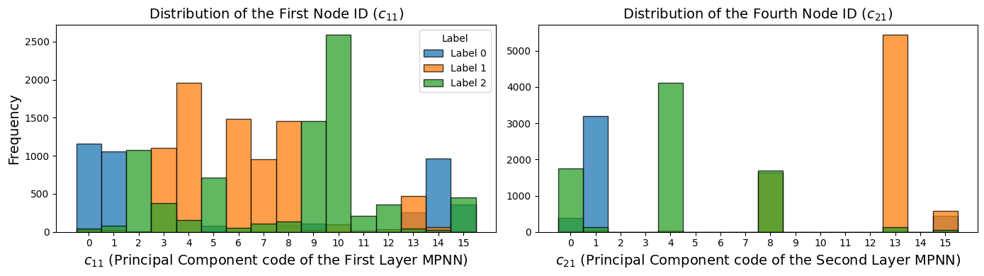
Figure 4: The codeword distributions of the $c_{11}$ and $c_{21}$ in PubMed colored by the ground-truth labels.

4.3 Node IDs Analysis

Table 9: Accuracy vs Inference Time.

	CiteSeer		ogbn-products
Metric	Acc$\uparrow$	Time$\downarrow$	Acc$\uparrow$	Time$\downarrow$
GCN	76.50	7.6ms	75.64	12.8s
VQGraph	76.28	1.3ms	79.17	1.6ms
NID	76.89	0.6ms	81.83	0.7ms

Table 10: Average GEDs of 1-hop subgraphs among nodes.

GEDs$\downarrow$	Cora	CiteSeer	PubMed
Random	7.21	4.83	9.61
VQGraph	6.85	4.73	9.03
NID	6.15	3.89	6.22

Table 11: Comparison of codebook usage rates (%).

Usage rate$\uparrow$	Cora	CiteSeer	PubMed
VQGraph	1.3	0.8	18.1
NID	84.7	97.9	79.1
$\textbf{NID}_{M\text{=}1}$	83.3	81.3	78.1

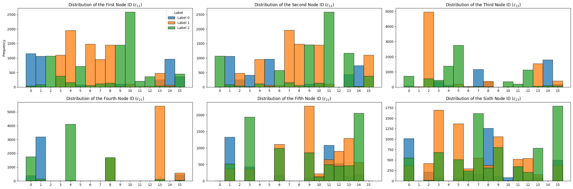
Figure 7: The codeword distributions of the node IDs in PubMed colored by the ground-truth labels.

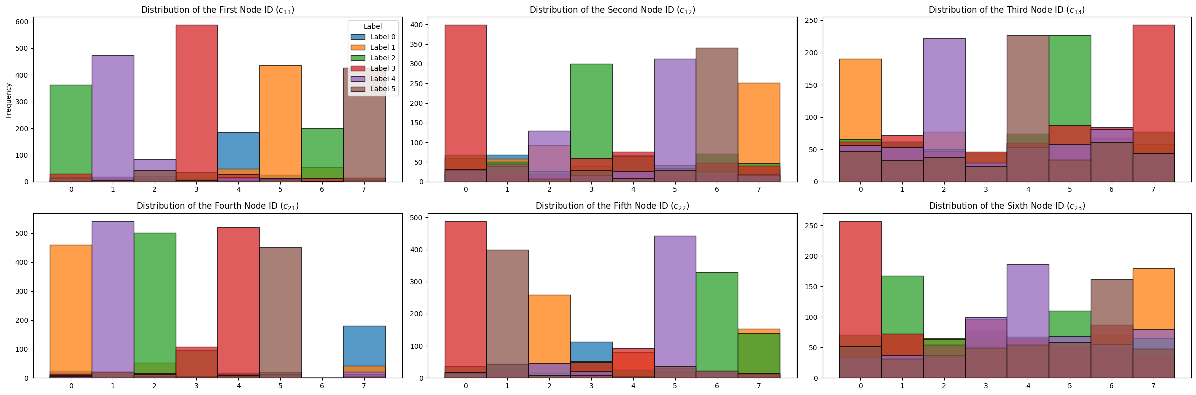
Figure 8: The codeword distributions of the node IDs in CiteSeer colored by the ground-truth labels.

Qualitative Analysis, Figures 4, 7, 8. We analyze the supervised node IDs for the PubMed dataset, depicted in Figures 4 & 7. The number of RVQ levels $M$ is set to 3, and the MPNN layers $L$ is set to 2, with a codebook size $K$ of 16. For a given node ID $\left(c_{11},c_{12},c_{13},c_{21},c_{22},c_{23}\right)$ of a node, $0\leq c_{lm}\leq 15$. The codes $c_{11}$ and $c_{21}$ capture the high-level information of the first and second MPNN layers, respectively. We present the distribution of $c_{11}$ and $c_{21}$ according to different labels. For instance, $c_{11}$ = 10 generally corresponds to label "2". Similarly, the majority of nodes with $c_{21}$ = 13 are labeled "1". Our node IDs have overlapping codewords for semantically similar labels, allowing the model to effectively share knowledge from semantically similar nodes in the dataset.

Acceleration in Inference Time, Table 11. We show the supervised node classification accuracy and model inference time on the CiteSeer and ogbn-products datasets in Table 11. Our results indicate that we achieve the highest accuracy of 76% and 81% while maintaining a fast inference time of 0.6ms and 0.7ms, respectively. Due to the ogbn-products dataset having over sixty million edges, graph loading is very slow. However, under the NID framework, we reduce the GCN inference time from 12.8s to 0.7ms, demonstrating a significant inference speedup of our approach in large networks.

Subgraph Retrieval, Table 11. We conduct node-centered subgraph retrieval using the supervised node IDs on the Cora, CiteSeer and PubMed. We identify the five nodes closest to a query node based on Hamming distances between their node IDs, then compute the average graph edit distance (GED) [89] between the 1-hop subgraph of the query node and the 1-hop subgraphs of these five nodes. The average GED across all nodes is detailed in Table 11. For comparison, we also calculate the GEDs using the VQGraph tokens and the randomly selected nodes. The results show that node IDs perform better in subgraph retrieval, with similar IDs more likely to exhibit similar structures.

High Codebook Usage, Table 11. We calculate the codebook usage rates for VQGraph tokenizer and NID. We find that VQGraph suffers from severe codebook collapse [15], where the majority of nodes are quantized into a small number of code vectors, leaving most of the codebook unused. In contrast, our NID achieves high codebook usage, effectively avoiding codebook collapse.

Figure 5: Ablation studies of codebook size, RVQ level and MPNNs layer; Supervised learning.

Ablation Study of the Codebook Size $K$, RVQ Level $M$ and MPNNs Layer $L$, Figure 5. First, we examine the influence of the codebook size $K$. The optimal $K$ varies across different graphs; however, generally, $K\leq 16$ yields the best performance on most datasets. A larger codebook size may lead to codebook collapse, impairing performance. Second, regarding the RVQ level $M$, we find that $M=3$ performs the best, which validates our fixed choice. Notably, when $M=1$, RVQ degenerates into VQ, which leads to decreased performance. Third, the number of MPNN layers required also differs based on the graph size. For instance, smaller graphs like CiteSeer perform well with just 2 layers, while larger graphs, such as ogbn-arxiv, may require more than 6 layers.

5 Related Works

Inference Acceleration for GNNs. GNNs are the preferred approach for representation learning on graph-structured data but suffer from decreased inference efficiency with larger graphs and more layers, particularly in real-time and resource-limited scenarios [40]. To mitigate this, three main strategies are employed [66]: knowledge distillation (e.g., GNN-to-GNN [115, 116] and GNN-to-MLP such as GraphMLP [36] and VQGraph [117]), pruning, (e.g., UGS [11] and Snowflake [102]), and quantization (e.g., VQ-GNN [16] and QLR [104]). Specifically, VQ-GNN utilizes vector quantization to efficiently compress message passing and maintain global context, while QLR applies low-bit quantization to reduce model size. It is worth noting that, our NID approach is uniquely different from VQGraph. While VQGraph focuses on learning node tokens through a reconstruction task for model distillation, our method simplifies node features into discrete node IDs, which can be directly used for prediction tasks with simple MLP layers.

Graph Tokenizers. In graph representation learning, significant strides have been made to vectorize structured data for downstream machine learning applications [7]. Early pioneering efforts like DeepWalk [79] and node2vec [28] popularized node embeddings, while subsequent research leveraged GNNs to generalize and learn node representations, effectively acting as graph tokenizers. These tokenizers have been instrumental across various applications such as molecular motifs [60, 87, 129], recommendation systems [94, 56], and knowledge graphs [93, 61]. The success of Large Language Models (LLMs) has also inspired recent explorations into applying tokenization concepts to graphs. Works such as InstructGLM [119], GraphText [130] and GPT4Graph [29] utilize natural language descriptions for graphs as tokens inputted to LLMs. Additionally, GraphToken [80] integrates tokens generated by GNNs with textual tokens to explicitly represent structured data for LLMs. However, these tokenizers often yield complex, high-dimensional embeddings. Recently, VQGraph [117] has employed a variant of VQ-VAE [98] to tokenize nodes as discrete codes. Our NID tokenizer offers significant advantages over the VQGraph tokenizer in 1) using multiple, small size codebooks to achieve a large representational capacity and avoid codebook collapse (Tab. 11) and 2) producing structure-aware semantic codes (IDs) that can reflect node similarity (Tab. 11, Fig. 1& 4).

6 Conclusions

We propose a novel graph tokenization framework, showcasing the potential to generate short, discrete codes, termed as node IDs, which serve as structure-informed, semantic node representations. Extensive experiments across various datasets and tasks confirm the effectiveness of node IDs, achieving competitive performance compared to SOTA methods and significantly improving efficiency.

Appendix A Self-supervised Node IDs using GraphCL

In this section, we discuss GraphCL [122] as a self-supervised learning (SSL) model for self-supervised Node IDs. Contrastive learning aims at learning an embedding space by comparing training samples and encouraging representations from positive pairs of examples to be close in the embedding space while representations from negative pairs are pushed away from each other. Such approaches usually consider each sample as its own class, that is, a positive pair consists of two different views of it; and all other samples in a batch are used as the negative pairs during training.

Specifically, a minibatch of $N$ graphs is randomly sampled and subjected to contrastive learning. This process results in $2N$ augmented graphs, along with a corresponding contrastive loss to be optimized. We redefine $\boldsymbol{z}_{n,i}$ and $\boldsymbol{z}_{n,j}$ for the $n$-th graph in the minibatch. Negative pairs are not explicitly sampled but are instead generated from the other $N-1$ augmented graphs within the same minibatch. The cosine similarity function is denoted as $\text{sim}(\boldsymbol{z}_{n,i},\boldsymbol{z}_{n,j})=\frac{\boldsymbol{z}_{n,i}^{T}\boldsymbol{z}_{n,j}}{\|\boldsymbol{z}_{n,i}\|\|\boldsymbol{z}_{n,j}\|}$. The NT-Xent loss [91] for the $n$-th graph is then defined as:

$$\mathcal{L}_{\text{GraphCL}}=-\log\frac{\exp(\text{sim}(\boldsymbol{z}_{n,i},\boldsymbol{z}_{n,j})/\tau)}{\sum_{n^{\prime}=1,n^{\prime}\neq n}^{N}\exp(\text{sim}(\boldsymbol{z}_{n,i},\boldsymbol{z}_{n^{\prime},j})/\tau)},$$

$$\boldsymbol{z}_{n,i}=\mathrm{R}\left(\text{MPNN}(v_{n,i},\boldsymbol{A}_{n,i},\boldsymbol{X}_{n,i})\right),$$

where $\tau$ represents the temperature parameter. The final loss is computed across all positive pairs in the minibatch. Consequently, Equation 7 is reformulated as:

$$\mathcal{L}_{\text{NID}}=\mathcal{L}_{\text{GraphCL}}+\sum_{n\in[1,N]}\sum_{v_{n,i}\in\mathcal{V}_{n,i}}\mathcal{L}_{\text{VQ}}(v_{n,i})+\sum_{v_{n,j}\in\mathcal{V}_{n,j}}\mathcal{L}_{\text{VQ}}(v_{n,j}),$$ (14)

Appendix B Datasets and Experimental Details

B.1 Computing Environment

Our implementation is based on PyG [21] and DGL [103]. The experiments are conducted on a single workstation with 8 RTX 3090 GPUs.

Table 12: Overview of the graph learning dataset used in this work [73, 19, 44, 12, 78, 88, 34, 71, 50, 72, 55, 81].

Dataset	# Graphs	Avg. # nodes	Avg. # edges	# Feats	Prediction level	Prediction task	Metric
NCI1	4,110	29.87	32.30	37	graph	2-class classif.	Accuracy
MUTAG	188	17.93	19.79	7	graph	2-class classif.	Accuracy
PROTEINS	1,113	39.06	72.82	3	graph	2-class classif.	Accuracy
DD	1,178	284.32	715.66	89	graph	2-class classif.	Accuracy
COLLAB	5,000	74.49	2457.78	1	graph	3-class classif.	Accuracy
REDDIT-BINARY	2,000	429.63	497.75	1	graph	2-class classif.	Accuracy
REDDIT-MULTI-5K	4,999	508.52	594.87	1	graph	5-class classif.	Accuracy
IMDB-BINARY	1,000	19.77	96.53	1	graph	2-class classif.	Accuracy
Peptides-func	15,535	150.9	307.3	9	graph	10-task classif.	AP
Peptides-struct	15,535	150.9	307.3	9	graph	11-task regression	MAE
ogbl-collab	1	235,868	1,285,465	128	edge	link prediction	Hits@50
ogbl-ppa	1	576,289	30,326,273	58	edge	link prediction	Hits@100
Cora	1	2,708	5,278	2,708	node	7-class classif.	Accuracy
Citeseer	1	3,327	4,522	3,703	node	6-class classif.	Accuracy
Pubmed	1	19,717	44,324	500	node	3-class classif.	Accuracy
Computer	1	13,752	245,861	767	node	10-class classif.	Accuracy
Photo	1	7,650	119,081	745	node	8-class classif.	Accuracy
CS	1	18,333	81,894	6,805	node	15-class classif.	Accuracy
Physics	1	34,493	247,962	8,415	node	5-class classif.	Accuracy
WikiCS	1	11,701	216,123	300	node	10-class classif.	Accuracy
Squirrel	1	5,201	216,933	2,089	node	5-class classif.	Accuracy
Chameleon	1	2,277	36,101	2,325	node	5-class classif.	Accuracy
Amazon-ratings	1	24,492	93,050	300	node	5-class classif.	Accuracy
ogbn-proteins	1	132,534	39,561,252	8	node	112 binary classif.	ROC-AUC
ogbn-arxiv	1	169,343	1,166,243	128	node	40-class classif.	Accuracy
ogbn-products	1	2,449,029	61,859,140	100	node	47-class classif.	Accuracy
pokec	1	1,632,803	30,622,564	65	node	binary classif.	Accuracy

B.2 Description of Datasets

Table 12 presents a summary of the statistics and characteristics of the datasets. The initial eight datasets are sourced from TUDataset [73], followed by two from LRGB [19], and finally the remaining datasets are obtained from [34, 44, 12, 78, 88, 71, 50, 72, 55, 81].

• Unsupervised Node Classification: Cora, Citeseer, Pubmed. For each dataset, we follow the standard splits and evaluation metrics in GraphMAE [33].

• Attributed Graph Clustering: Cora, Citeseer. To evaluate the clustering performance, we adopt three performance measures: clustering accuracy (Acc), normalized mutual information (NMI), and macro F1-score (F1), following the approach used in AGC [128].

• Unsupervised Graph Classification: NCI1, PROTEINS, DD, MUTAG, COLLAB, REDDIT-B, REDDIT-M5K, and IMDB-B. Each dataset is a collection of graphs where each graph is associated with a label. Each dataset consists of a set of graphs, with each graph associated with a label. For NCI1, PROTEINS, DD, and MUTAG, node labels serve as input features, while for COLLAB, REDDIT-B, REDDIT-M5K, and IMDB-B, node degrees are utilized. In each dataset, we follow exactly the same data splits and evaluation metircs as the standard settings [122].

• Supervised Node Classification: Cora, Citeseer, Pubmed, Computer, Photo, CS, Physics, WikiCS, Amazon-ratings, Squirrel, Chameleon, ogbn-proteins, ogbn-arxiv, ogbn-products and pokec. For Cora, Citeseer, and Pubmed, we employ a training/validation/testing split ratio of 60%/20%/20% and use accuracy as the evaluation metric, consistent with [78]. For Squirrel and Chameleon, we adhere to the standard splits and evaluation metrics outlined in [108]. For the remaining datasets, standard splits and metrics are followed as specified in [14]. For comprehensive details on these datasets, please refer to the respective studies [78, 108, 14].

• Supervised Link Prediction: Cora, Citeseer, Pubmed, ogbl-collab and ogbl-ppa. We follow the standard splits and evaluation metrics specified in [105], with further details provided therein.

• Supervised Graph Classification: Peptides-func and Peptides-struct. For each dataset, we follow the standard train/validation/test splits and evaluation metrics in [83]. For more comprehensive details, readers are encouraged to refer to [83].

B.3 Baselines

Unsupervised Node Classification. We utilize all the baselines from GraphMAE [33]: GAE [43], DGI [100], MVGRL [31], InfoGCL [113], CCA-SSG[125] and GraphMAE [33].

Attributed Graph Clustering. We apply baseline methods from AGC [128]: DeepWalk [79], GAE [43], MGAE [101], ARGE [77], AGC [128], GraphMAE [33]. For $k$-means, it refers to clustering directly based on node features.

Unsupervised Graph Classification. We utilize the baselines from GraphCL [122]: graphlet kernel (GL), Weisfeiler-Lehman sub-tree kernel (WL), deep graph kernel (DGK), graph2vec [76], InfoGraph [92], GraphCL [122], EdgePred [35], ContextPred [35], AttrMask [35], SimGRACE [111] and JOAO [121].

Supervised Node Classification. We compare our method to the following prevalent GNNs and transformer models from Polynormer [14]: GCN [44], SAGE [30], GAT [99], APPNP [25], GPRGNN [12], H2GCN [132], GCNII [10], FSGNN [70], GloGNN [54], tGNN [37], LINKX [55], NodeFormer [107], GOAT [45], NAGphormer [9], Exphormer [90], DIFFormer [106], GraphGPS [83], Polynormer [14], SGFormer [108].

Supervised Link Prediction. We employ all the baselines from NCN [105]: GCN [44], SAGE [30], SEAL [126], NBFnet [133], Neo-GNN [123], BUDDY [6], NCN [105].

Supervised Graph Classification. We compare our method to the following prevalent GNNs: GCN [44], and GatedGCN [3]. In terms of transformer models, we consider GT[17], Graph ViT [32], Exphormer [90], GraphGPS [83], and GRIT [65].

We report the performance of baseline models using results from their original papers or official leaderboards, where available, as these are derived from well-tuned configurations. For baselines without publicly available results on specific datasets, we adjust their hyperparameters, conducting a search within the parameter space defined in the original papers, to attain the highest possible accuracy.

B.4 Hyperparameters and Reproducibility

RVQ Implementation Details. We fix the RVQ level to $M=3$. In our experiments, cosine similarity serves as the distance metric $||\cdot||$ within the RVQ framework. The codebook size $K$ is optimized over the set {4, 6, 8, 16, 32}. The parameter $\beta$ is fixed at 1.

For the hyperparameter selections of our NID framework, in addition to what we have covered, we list other settings in Table 13. The tasks are presented in the following order: unsupervised node classification, attribute graph clustering, unsupervised graph classification, supervised node classification, supervised link prediction, and supervised graph classification. Below we detail the experimental settings for pretraining the node ID.

Table 13: Dataset-specific hyperparameter settings of NID framework.

Dataset	Codebook size $K$	MPNN	MPNNs layer $L$	Hidden dim	LR	epoch	MLP layer
Cora	32	GAT	2	1024	0.001	1500	3
Citeseer	8	GAT	2	256	0.001	500	3
Pubmed	16	GAT	2	128	0.0005	500	3
Cora	8	GAT	2	1024	0.001	1500	3
Citeseer	8	GAT	2	256	0.001	500	3
NCI1	4	GIN	5	32	0.01	20	SVM
MUTAG	16	GIN	4	32	0.01	20	SVM
PROTEINS	8	GIN	3	32	0.01	20	SVM
DD	4	GIN	4	32	0.01	20	SVM
COLLAB	32	GIN	5	32	0.01	20	SVM
REDDIT-BINARY	4	GIN	5	32	0.01	20	SVM
REDDIT-MULTI-5K	4	GIN	4	32	0.01	20	SVM
IMDB-BINARY	8	GIN	3	32	0.01	20	SVM
Cora	6	GCN	4	128	0.01	1000	5
Citeseer	8	GCN	2	128	0.01	1000	5
Pubmed	16	GCN	2	256	0.005	1000	5
Computer	8	GAT	6	64	0.001	1200	5
Photo	4	GAT	6	64	0.001	1200	4
CS	16	GAT	7	64	0.001	1600	4
Physics	4	GAT	8	32	0.001	1600	4
WikiCS	8	GAT	8	512	0.001	1000	4
Squirrel	32	GCN	5	128	0.01	500	3
Chameleon	16	GCN	3	64	0.01	500	2
Amazon-ratings	16	GAT	12	256	0.001	2500	4
ogbn-proteins	4	SAGE	4	256	0.0005	1000	5
ogbn-arxiv	16	GAT	7	256	0.0005	2000	4
ogbn-products	16	SAGE	5	128	0.003	1000	4
pokec	16	GAT	7	256	0.0005	2000	5
Cora	32	GCN	10	256	0.004	150	3
Citeseer	8	GCN	10	256	0.01	10	3
Pubmed	8	GCN	10	256	0.01	100	3
ogbl-collab	16	GCN	5	256	0.001	150	3
ogbl-ppa	16	GCN	5	64	0.001	200	3
Peptides-func	16	GCN	6	235	0.001	500	5
Peptides-struct	16	GCN	6	235	0.001	250	5

Unsupervised Node Classification and Attributed Graph Clustering. The pretraining hyperparameters are selected within the GraphMAE’s grid search space, as outlined in Table 13. All other experimental parameters, including dropout, batch size, training schemes, and optimizer, etc., align with those used in GraphMAE [33].

Unsupervised Graph Classification. Similarly, our pretraining hyperparameters in table are determined within GraphCL’s grid search space. All other experimental parameters match those used in GraphCL [122]. Specially for this task, following GraphCL [122], we input $\textbf{NID}_{\text{CL}}$ codes into a downstream LIBSVM [8] classifier. And models are trained for 20 epochs and tested every 10 epochs. We conduct a 10-fold cross-validation on every dataset. For each fold, we utilize 90% of the total data as the unlabeled data and the remaining 10% as the labeled testing data. Every experiment is repeated 5 times using different random seeds, with mean and standard deviation of accuracies (%) reported.

Supervised Node Classification. Pretraining hyperparameters in table for this task are derived from Polynormer’s grid search space. All other experimental parameters are aligned with those used in Polynormer [14].

Supervised Link Prediction. Our pretraining hyperparameters in table are chosen from the NCN’s grid search space. All other experimental parameters match those used in NCN [105]. For the Cora, CiteSeer, and PubMed datasets, we employ the Hadamard product as the readout function. For ogbl-collab and ogbl-ppa, we use sum pooling on the node IDs of the $1$-hop common neighbors [2] to nodes $u$ and $v$ for the edge $(u,v)$, expressed as $\sum_{w\in\mathcal{N}(v)\cap\mathcal{N}(u)}\text{Node\_ID}(w)$.

Supervised Graph Classification. All experimental parameters are consistent with those used in the [97].

Applications of Node IDs for Graph Learning. After obtaining the ID, we train the Multi-Layer Perceptron (MLP) for different tasks, with the number of layers specified in Table 13 and hidden dimensions of either 256 or 512. We utilize the Adam optimizer [42] with the default settings. We set a learning rate of either 0.01 or 0.001 and an epoch limit of 1000. The ReLU function serves as the non-linear activation. Further details regarding hyperparameters can be found in the code in the supplementary material. In all experiments, we use the validation set to select the best hyperparameters. All results are derived from 10 independent runs, with mean and standard deviation of results reported.

Appendix C Additional Benchmark Results

C.1 Impact of the Ratio of Training Set

Figure 6: Node classification results of NID in supervised learning across various training set ratios.

C.2 Qualitative Analysis

C.3 Additional Linear Probing

Datasets. To evaluate the transferability of the proposed method, we test the performance through linear probing on molecular property prediction, adhering to the settings described by [122]. Initially, the $\textbf{NID}_{\text{CL}}$ is pre-trained on 2 million unlabeled molecules sourced from ZINC15 [35].

• Node features:

  • Atom number: $[1,118]$

  • Chirality tag: $\{$unspecified, tetrahedral cw, tetrahedral ccw, other$\}$

• Edge features:

  • Bond type: $\{$single, double, triple, aromatic$\}$

  • Bond direction: $\{$–, endupright, enddownright$\}$

Then, we focus on molecular property prediction, where we adopt the widely-used 7 binary classification datasets contained in MoleculeNet [110] for linear probing. The scaffold-split [84] is used to split downstream dataset graphs into training/validation/testing set as 80%/10%/10% which mimics real-world use cases. For the evaluation protocol, we run experiments for 10 times and report the mean and standard deviation of ROC-AUC scores (%).

Model Hyperparameters. Following [122], we adopt a 5-layer GIN [114] with a 300 hidden dimension as the MPNN architecture, and set the RVQ codebook size at $K=16$. We use mean pooling as the readout function. During the pre-training stage, GIN is pre-trained for 100 epochs with batch-size as 256 and the learning rate as 0.001. After the model is trained on the pre-training dataset, it is directly applied to the downstream dataset to obtain node IDs. To evaluate the learned node IDs, we follow the linear probing (linear evaluation) [1], where a linear classifier (1 linear layer) is trained on the node IDs. During the probing stage, we train for 100 epochs with batch-size as 32, dropout rate as 0.5, and report the test performance using ROC-AUC at the best validation epoch.

The results are presented in Table 14. It is noteworthy that $\textbf{NID}_{\text{CL}}$ outperforms the baselines in the SIDER, ClinTox, and BBBP datasets, and shows significant improvement over the embeddings from GraphCL. This suggests the robust transferability of $\textbf{NID}_{\text{CL}}$.

Table 14: Linear probing: molecular property prediction; binary classification, ROC-AUC (%).

	Tox21	ToxCast	Sider	ClinTox	HIV	BBBP	Bace
EdgePred	62.7 ± 0.6	55.3 ± 0.4	51.0 ± 0.3	48.9 ± 6.5	64.9 ± 2.0	54.8 ± 0.7	68.8 ± 0.9
ContextPred	68.4 ± 0.3	59.1 ± 0.2	59.4 ± 0.3	43.2 ± 1.7	68.9 ± 0.4	59.1 ± 0.2	64.4 ± 0.6
AttrMask	69.1 ± 0.2	58.2 ± 0.2	51.7 ± 0.1	51.6 ± 0.7	60.9 ± 1.3	61.0 ± 1.3	64.4 ± 2.5
JOAO	70.6 ± 0.4	60.5 ± 0.3	57.4 ± 0.6	54.1 ± 2.6	68.1 ± 0.9	63.7 ± 0.3	71.2 ± 1.0
SimGRACE	64.6 ± 0.4	59.1 ± 0.2	54.9 ± 0.6	63.4 ± 2.6	66.3 ± 1.5	65.4 ± 1.2	67.8 ± 1.3
GraphCL	64.4 ± 0.5	59.4 ± 0.2	54.6 ± 0.3	59.8 ± 1.2	63.7 ± 2.3	62.4 ± 0.7	71.1 ± 0.7
$\textbf{NID}_{\text{CL}}$	66.3 ± 0.4	59.1 ± 0.3	60.1 ± 0.4	65.3 ± 2.2	64.3 ± 0.8	66.9 ± 0.6	66.1 ± 1.2

C.4 Additional Comparison Results with VQGraph Tokens

In this section, we specifically compare the node classification results with VQGraph tokens under the same experimental settings. VQGraph tokens refers to training an MLP with tokens learned by VQGraph tokenizer from [117]. As shown in Table 15, VQGraph tokens lack semantic information, likely due to codebook collapse encountered by their tokenizer (see Table 11).

Table 15: Node classification results in supervised representation learning.

	Cora	CiteSeer	PubMed	ogbn-arxiv
Metric	Accuracy$\uparrow$	Accuracy$\uparrow$	Accuracy$\uparrow$	Accuracy$\uparrow$
VQGraph tokens	63.39 ± 1.15	32.07 ± 2.70	54.37 ± 4.76	43.57 ± 0.49
NID	87.88 ± 0.69	76.89 ± 1.09	89.42 ± 0.44	71.27 ± 0.24

Appendix D Limitations & Broader Impacts

Broader Impacts. This paper presents work whose goal is to advance the field of Machine Learning. There are many potential societal consequences of our work, none which we feel must be specifically highlighted here.

Limitations. Our node IDs have proven to be effective in large-scale graphs by accelerating clustering and inference processes due to their low-dimensional nature. However, we have found that the number of available datasets for very large networks is limited, and we acknowledge that there is still room for extension. Additionally, we believe that node IDs could benefit large language models, a topic we intend to explore more extensively in our future work.

Appendix E Further Related Works

Vector Quantization (VQ). VQ compresses the representation space into a compact codebook of multiple codewords, using a single code to approximate each vector [57]. Advanced methods like VQ-VAE [98] and RQ-VAE [49] enhance quantization precision by employing multiple codebooks, initially for image generation and later adapted to recommender systems [82, 58] and multimodal representation learning [131, 112]. This paper introduces residual quantization for learning structure-aware semantic node IDs, achieving superior feature compression performance.

Positional Encodings (PEs) as Graph Tokens. Transformer models with attention mechanisms can process graphs by tokenizing nodes and edges, incorporating positional or structural graph information through PEs [75]. The Graph Transformer [17] and SAN [47] initially employed Laplacian eigenvectors as PEs. Subsequent models like LSPE [19] utilized random walk probabilities as node tokens. TokenGT [41] introduced orthogonal vectors for both node and edge tokens, and follow-up works also consider larger graphs [63, 64]. However, these methods primarily encode the structural information of the graph and overlook the semantic details of nodes, thereby constraining their direct application.

References

- [1] Mohammad Sadegh Akhondzadeh, Vijay Lingam, and Aleksandar Bojchevski. Probing graph representations. In Francisco Ruiz, Jennifer Dy, and Jan-Willem van de Meent, editors, Proceedings of The 26th International Conference on Artificial Intelligence and Statistics, volume 206 of Proceedings of Machine Learning Research, pages 11630–11649. PMLR, 25–27 Apr 2023.
- [2] Albert-László Barabási and Réka Albert. Emergence of scaling in random networks. science, 286(5439):509–512, 1999.
- [3] Xavier Bresson and Thomas Laurent. Residual gated graph convnets. arXiv preprint arXiv:1711.07553, 2017.
- [4] Joan Bruna, Wojciech Zaremba, Arthur Szlam, and Yann LeCun. Spectral networks and locally connected networks on graphs. arXiv preprint arXiv:1312.6203, 2013.
- [5] Hongyun Cai, Vincent W Zheng, and Kevin Chen-Chuan Chang. A comprehensive survey of graph embedding: Problems, techniques, and applications. IEEE transactions on knowledge and data engineering, 30(9):1616–1637, 2018.
- [6] Benjamin Paul Chamberlain, Sergey Shirobokov, Emanuele Rossi, Fabrizio Frasca, Thomas Markovich, Nils Yannick Hammerla, Michael M Bronstein, and Max Hansmire. Graph neural networks for link prediction with subgraph sketching. In The eleventh international conference on learning representations, 2022.
- [7] Ines Chami, Sami Abu-El-Haija, Bryan Perozzi, Christopher Ré, and Kevin Murphy. Machine learning on graphs: A model and comprehensive taxonomy. Journal of Machine Learning Research, 23(89):1–64, 2022.
- [8] Chih-Chung Chang and Chih-Jen Lin. Libsvm: a library for support vector machines. ACM transactions on intelligent systems and technology (TIST), 2(3):1–27, 2011.
- [9] Jinsong Chen, Kaiyuan Gao, Gaichao Li, and Kun He. Nagphormer: A tokenized graph transformer for node classification in large graphs. In The Eleventh International Conference on Learning Representations, 2022.
- [10] Ming Chen, Zhewei Wei, Zengfeng Huang, Bolin Ding, and Yaliang Li. Simple and deep graph convolutional networks. In International conference on machine learning, pages 1725–1735. PMLR, 2020.
- [11] Tianlong Chen, Yongduo Sui, Xuxi Chen, Aston Zhang, and Zhangyang Wang. A unified lottery ticket hypothesis for graph neural networks. In International conference on machine learning, pages 1695–1706. PMLR, 2021.
- [12] Eli Chien, Jianhao Peng, Pan Li, and Olgica Milenkovic. Adaptive universal generalized pagerank graph neural network. In International Conference on Learning Representations, 2020.
- [13] Michaël Defferrard, Xavier Bresson, and Pierre Vandergheynst. Convolutional neural networks on graphs with fast localized spectral filtering. Advances in neural information processing systems, 29, 2016.
- [14] Chenhui Deng, Zichao Yue, and Zhiru Zhang. Polynormer: Polynomial-expressive graph transformer in linear time. arXiv preprint arXiv:2403.01232, 2024.
- [15] Prafulla Dhariwal, Heewoo Jun, Christine Payne, Jong Wook Kim, Alec Radford, and Ilya Sutskever. Jukebox: A generative model for music. arXiv preprint arXiv:2005.00341, 2020.
- [16] Mucong Ding, Kezhi Kong, Jingling Li, Chen Zhu, John Dickerson, Furong Huang, and Tom Goldstein. Vq-gnn: A universal framework to scale up graph neural networks using vector quantization. Advances in Neural Information Processing Systems, 34:6733–6746, 2021.
- [17] Vijay Prakash Dwivedi and Xavier Bresson. A generalization of transformer networks to graphs. arXiv preprint arXiv:2012.09699, 2020.
- [18] Vijay Prakash Dwivedi, Chaitanya K Joshi, Anh Tuan Luu, Thomas Laurent, Yoshua Bengio, and Xavier Bresson. Benchmarking graph neural networks. Journal of Machine Learning Research, 24(43):1–48, 2023.
- [19] Vijay Prakash Dwivedi, Ladislav Rampášek, Mikhail Galkin, Ali Parviz, Guy Wolf, Anh Tuan Luu, and Dominique Beaini. Long range graph benchmark. arXiv preprint arXiv:2206.08164, 2022.
- [20] Wenqi Fan, Yao Ma, Qing Li, Yuan He, Eric Zhao, Jiliang Tang, and Dawei Yin. Graph neural networks for social recommendation. In The world wide web conference, pages 417–426, 2019.
- [21] Matthias Fey and Jan Eric Lenssen. Fast graph representation learning with pytorch geometric. arXiv preprint arXiv:1903.02428, 2019.
- [22] Santo Fortunato. Community detection in graphs. Physics reports, 486(3-5):75–174, 2010.
- [23] Santo Fortunato and Darko Hric. Community detection in networks: A user guide. Physics reports, 659:1–44, 2016.
- [24] Keinosuke Fukunaga and Larry Hostetler. The estimation of the gradient of a density function, with applications in pattern recognition. IEEE Transactions on information theory, 21(1):32–40, 1975.
- [25] Johannes Gasteiger, Aleksandar Bojchevski, and Stephan Günnemann. Predict then propagate: Graph neural networks meet personalized pagerank. arXiv preprint arXiv:1810.05997, 2018.
- [26] Justin Gilmer, Samuel S Schoenholz, Patrick F Riley, Oriol Vinyals, and George E Dahl. Neural message passing for quantum chemistry. In International conference on machine learning, pages 1263–1272. PMLR, 2017.
- [27] Robert Gray. Vector quantization. IEEE Assp Magazine, 1(2):4–29, 1984.
- [28] Aditya Grover and Jure Leskovec. node2vec: Scalable feature learning for networks. In Proceedings of the 22nd ACM SIGKDD international conference on Knowledge discovery and data mining, pages 855–864, 2016.
- [29] Jiayan Guo, Lun Du, and Hengyu Liu. Gpt4graph: Can large language models understand graph structured data? an empirical evaluation and benchmarking. arXiv preprint arXiv:2305.15066, 2023.
- [30] Will Hamilton, Zhitao Ying, and Jure Leskovec. Inductive representation learning on large graphs. Advances in neural information processing systems, 30, 2017.
- [31] Kaveh Hassani and Amir Hosein Khasahmadi. Contrastive multi-view representation learning on graphs. In International conference on machine learning, pages 4116–4126. PMLR, 2020.
- [32] Xiaoxin He, Bryan Hooi, Thomas Laurent, Adam Perold, Yann LeCun, and Xavier Bresson. A generalization of vit/mlp-mixer to graphs. In International Conference on Machine Learning, pages 12724–12745. PMLR, 2023.
- [33] Zhenyu Hou, Xiao Liu, Yukuo Cen, Yuxiao Dong, Hongxia Yang, Chunjie Wang, and Jie Tang. Graphmae: Self-supervised masked graph autoencoders. In Proceedings of the 28th ACM SIGKDD Conference on Knowledge Discovery and Data Mining, pages 594–604, 2022.
- [34] Weihua Hu, Matthias Fey, Marinka Zitnik, Yuxiao Dong, Hongyu Ren, Bowen Liu, Michele Catasta, and Jure Leskovec. Open graph benchmark: Datasets for machine learning on graphs. Advances in neural information processing systems, 33:22118–22133, 2020.
- [35] Weihua Hu*, Bowen Liu*, Joseph Gomes, Marinka Zitnik, Percy Liang, Vijay Pande, and Jure Leskovec. Strategies for pre-training graph neural networks. In International Conference on Learning Representations, 2020.
- [36] Yang Hu, Haoxuan You, Zhecan Wang, Zhicheng Wang, Erjin Zhou, and Yue Gao. Graph-mlp: Node classification without message passing in graph. arXiv preprint arXiv:2106.04051, 2021.
- [37] Chenqing Hua, Guillaume Rabusseau, and Jian Tang. High-order pooling for graph neural networks with tensor decomposition. Advances in Neural Information Processing Systems, 35:6021–6033, 2022.
- [38] Zhihao Jia, Sina Lin, Rex Ying, Jiaxuan You, Jure Leskovec, and Alex Aiken. Redundancy-free computation for graph neural networks. In Proceedings of the 26th ACM SIGKDD International Conference on Knowledge Discovery & Data Mining, pages 997–1005, 2020.
- [39] Biing-Hwang Juang and A Gray. Multiple stage vector quantization for speech coding. In ICASSP’82. IEEE International Conference on Acoustics, Speech, and Signal Processing, volume 7, pages 597–600. IEEE, 1982.
- [40] Tim Kaler, Nickolas Stathas, Anne Ouyang, Alexandros-Stavros Iliopoulos, Tao Schardl, Charles E Leiserson, and Jie Chen. Accelerating training and inference of graph neural networks with fast sampling and pipelining. Proceedings of Machine Learning and Systems, 4:172–189, 2022.
- [41] Jinwoo Kim, Dat Nguyen, Seonwoo Min, Sungjun Cho, Moontae Lee, Honglak Lee, and Seunghoon Hong. Pure transformers are powerful graph learners. Advances in Neural Information Processing Systems, 35:14582–14595, 2022.
- [42] Diederik P Kingma and Jimmy Ba. Adam: A method for stochastic optimization. arXiv preprint arXiv:1412.6980, 2014.
- [43] Thomas N Kipf and Max Welling. Variational graph auto-encoders. arXiv preprint arXiv:1611.07308, 2016.
- [44] Thomas N. Kipf and Max Welling. Semi-supervised classification with graph convolutional networks. In International Conference on Learning Representations, 2017.
- [45] Kezhi Kong, Jiuhai Chen, John Kirchenbauer, Renkun Ni, C. Bayan Bruss, and Tom Goldstein. GOAT: A global transformer on large-scale graphs. In Andreas Krause, Emma Brunskill, Kyunghyun Cho, Barbara Engelhardt, Sivan Sabato, and Jonathan Scarlett, editors, Proceedings of the 40th International Conference on Machine Learning, volume 202 of Proceedings of Machine Learning Research, pages 17375–17390. PMLR, 23–29 Jul 2023.
- [46] Ioannis Konstas, Vassilios Stathopoulos, and Joemon M Jose. On social networks and collaborative recommendation. In Proceedings of the 32nd international ACM SIGIR conference on Research and development in information retrieval, pages 195–202, 2009.
- [47] Devin Kreuzer, Dominique Beaini, Will Hamilton, Vincent Létourneau, and Prudencio Tossou. Rethinking graph transformers with spectral attention. Advances in Neural Information Processing Systems, 34:21618–21629, 2021.
- [48] Luís C Lamb, Artur d’Avila Garcez, Marco Gori, Marcelo OR Prates, Pedro HC Avelar, and Moshe Y Vardi. Graph neural networks meet neural-symbolic computing: a survey and perspective. In Proceedings of the Twenty-Ninth International Conference on International Joint Conferences on Artificial Intelligence, pages 4877–4884, 2021.
- [49] Doyup Lee, Chiheon Kim, Saehoon Kim, Minsu Cho, and Wook-Shin Han. Autoregressive image generation using residual quantization. In Proceedings of the IEEE/CVF Conference on Computer Vision and Pattern Recognition, pages 11523–11532, 2022.
- [50] Jure Leskovec and Andrej Krevl. Snap datasets: Stanford large network dataset collection. 2014. 2016.
- [51] Guohao Li, Matthias Muller, Ali Thabet, and Bernard Ghanem. Deepgcns: Can gcns go as deep as cnns? In Proceedings of the IEEE/CVF international conference on computer vision, pages 9267–9276, 2019.
- [52] Qimai Li, Zhichao Han, and Xiao-Ming Wu. Deeper insights into graph convolutional networks for semi-supervised learning. In Thirty-Second AAAI conference on artificial intelligence, 2018.
- [53] Qimai Li, Xiao-Ming Wu, Han Liu, Xiaotong Zhang, and Zhichao Guan. Label efficient semi-supervised learning via graph filtering. In Proceedings of the IEEE/CVF conference on computer vision and pattern recognition, pages 9582–9591, 2019.
- [54] Xiang Li, Renyu Zhu, Yao Cheng, Caihua Shan, Siqiang Luo, Dongsheng Li, and Weining Qian. Finding global homophily in graph neural networks when meeting heterophily. In International Conference on Machine Learning, pages 13242–13256. PMLR, 2022.
- [55] Derek Lim, Felix Hohne, Xiuyu Li, Sijia Linda Huang, Vaishnavi Gupta, Omkar Bhalerao, and Ser Nam Lim. Large scale learning on non-homophilous graphs: New benchmarks and strong simple methods. Advances in Neural Information Processing Systems, 34:20887–20902, 2021.
- [56] Han Liu, Yinwei Wei, Xuemeng Song, Weili Guan, Yuan-Fang Li, and Liqiang Nie. Mmgrec: Multimodal generative recommendation with transformer model. arXiv preprint arXiv:2404.16555, 2024.
- [57] Qijiong Liu, Xiaoyu Dong, Jiaren Xiao, Nuo Chen, Hengchang Hu, Jieming Zhu, Chenxu Zhu, Tetsuya Sakai, and Xiao-Ming Wu. Vector quantization for recommender systems: A review and outlook. arXiv preprint arXiv:2405.03110, 2024.
- [58] Qijiong Liu, Hengchang Hu, Jiahao Wu, Jieming Zhu, Min-Yen Kan, and Xiao-Ming Wu. Discrete semantic tokenization for deep ctr prediction. arXiv preprint arXiv:2403.08206, 2024.
- [59] Xiao Liu, Fanjin Zhang, Zhenyu Hou, Li Mian, Zhaoyu Wang, Jing Zhang, and Jie Tang. Self-supervised learning: Generative or contrastive. IEEE transactions on knowledge and data engineering, 35(1):857–876, 2021.
- [60] Zhiyuan Liu, Yaorui Shi, An Zhang, Enzhi Zhang, Kenji Kawaguchi, Xiang Wang, and Tat-Seng Chua. Rethinking tokenizer and decoder in masked graph modeling for molecules. Advances in Neural Information Processing Systems, 36, 2024.
- [61] Yunzhong Lou, Xueyang Li, Haotian Chen, and Xiangdong Zhou. Brep-bert: Pre-training boundary representation bert with sub-graph node contrastive learning. In Proceedings of the 32nd ACM International Conference on Information and Knowledge Management, pages 1657–1666, 2023.
- [62] Linyuan Lü and Tao Zhou. Link prediction in complex networks: A survey. Physica A: statistical mechanics and its applications, 390(6):1150–1170, 2011.
- [63] Yuankai Luo. Transformers for capturing multi-level graph structure using hierarchical distances. arXiv preprint arXiv:2308.11129, 2023.
- [64] Yuankai Luo, Veronika Thost, and Lei Shi. Transformers over directed acyclic graphs. Advances in Neural Information Processing Systems, 36, 2024.
- [65] Liheng Ma, Chen Lin, Derek Lim, Adriana Romero-Soriano, Puneet K Dokania, Mark Coates, Philip Torr, and Ser-Nam Lim. Graph inductive biases in transformers without message passing. arXiv preprint arXiv:2305.17589, 2023.
- [66] Lu Ma, Zeang Sheng, Xunkai Li, Xinyi Gao, Zhezheng Hao, Ling Yang, Wentao Zhang, and Bin Cui. Acceleration algorithms in gnns: A survey. arXiv preprint arXiv:2405.04114, 2024.
- [67] James MacQueen et al. Some methods for classification and analysis of multivariate observations. In Proceedings of the fifth Berkeley symposium on mathematical statistics and probability, volume 1, pages 281–297. Oakland, CA, USA, 1967.
- [68] John Makhoul, Salim Roucos, and Herbert Gish. Vector quantization in speech coding. Proceedings of the IEEE, 73(11):1551–1588, 1985.
- [69] Julieta Martinez, Holger H Hoos, and James J Little. Stacked quantizers for compositional vector compression. arXiv preprint arXiv:1411.2173, 2014.
- [70] Sunil Kumar Maurya, Xin Liu, and Tsuyoshi Murata. Improving graph neural networks with simple architecture design. arXiv preprint arXiv:2105.07634, 2021.
- [71] Julian McAuley, Rahul Pandey, and Jure Leskovec. Inferring networks of substitutable and complementary products. In Proceedings of the 21th ACM SIGKDD international conference on knowledge discovery and data mining, pages 785–794, 2015.
- [72] Péter Mernyei and Cătălina Cangea. Wiki-cs: A wikipedia-based benchmark for graph neural networks. arXiv preprint arXiv:2007.02901, 2020.
- [73] Christopher Morris, Nils M Kriege, Franka Bause, Kristian Kersting, Petra Mutzel, and Marion Neumann. Tudataset: A collection of benchmark datasets for learning with graphs. arXiv preprint arXiv:2007.08663, 2020.
- [74] Christopher Morris, Martin Ritzert, Matthias Fey, William L Hamilton, Jan Eric Lenssen, Gaurav Rattan, and Martin Grohe. Weisfeiler and leman go neural: Higher-order graph neural networks. In Proceedings of the AAAI conference on artificial intelligence, volume 33, pages 4602–4609, 2019.
- [75] Luis Müller, Mikhail Galkin, Christopher Morris, and Ladislav Rampášek. Attending to graph transformers. arXiv preprint arXiv:2302.04181, 2023.
- [76] Annamalai Narayanan, Mahinthan Chandramohan, Rajasekar Venkatesan, Lihui Chen, Yang Liu, and Shantanu Jaiswal. graph2vec: Learning distributed representations of graphs. arXiv preprint arXiv:1707.05005, 2017.
- [77] Shirui Pan, Ruiqi Hu, Guodong Long, Jing Jiang, Lina Yao, and Chengqi Zhang. Adversarially regularized graph autoencoder for graph embedding. arXiv preprint arXiv:1802.04407, 2018.
- [78] Hongbin Pei, Bingzhe Wei, Kevin Chen-Chuan Chang, Yu Lei, and Bo Yang. Geom-gcn: Geometric graph convolutional networks. In International Conference on Learning Representations, 2019.
- [79] Bryan Perozzi, Rami Al-Rfou, and Steven Skiena. Deepwalk: Online learning of social representations. In Proceedings of the 20th ACM SIGKDD international conference on Knowledge discovery and data mining, pages 701–710, 2014.
- [80] Bryan Perozzi, Bahare Fatemi, Dustin Zelle, Anton Tsitsulin, Mehran Kazemi, Rami Al-Rfou, and Jonathan Halcrow. Let your graph do the talking: Encoding structured data for llms. arXiv preprint arXiv:2402.05862, 2024.
- [81] Oleg Platonov, Denis Kuznedelev, Michael Diskin, Artem Babenko, and Liudmila Prokhorenkova. A critical look at the evaluation of gnns under heterophily: Are we really making progress? arXiv preprint arXiv:2302.11640, 2023.
- [82] Shashank Rajput, Nikhil Mehta, Anima Singh, Raghunandan Hulikal Keshavan, Trung Vu, Lukasz Heldt, Lichan Hong, Yi Tay, Vinh Tran, Jonah Samost, et al. Recommender systems with generative retrieval. Advances in Neural Information Processing Systems, 36, 2024.
- [83] Ladislav Rampášek, Mikhail Galkin, Vijay Prakash Dwivedi, Anh Tuan Luu, Guy Wolf, and Dominique Beaini. Recipe for a general, powerful, scalable graph transformer. arXiv preprint arXiv:2205.12454, 2022.
- [84] Bharath Ramsundar, Peter Eastman, Patrick Walters, and Vijay Pande. Deep learning for the life sciences: applying deep learning to genomics, microscopy, drug discovery, and more. O’Reilly Media, 2019.
- [85] Ali Razavi, Aaron Van den Oord, and Oriol Vinyals. Generating diverse high-fidelity images with vq-vae-2. Advances in neural information processing systems, 32, 2019.
- [86] Patrick Reiser, Marlen Neubert, André Eberhard, Luca Torresi, Chen Zhou, Chen Shao, Houssam Metni, Clint van Hoesel, Henrik Schopmans, Timo Sommer, et al. Graph neural networks for materials science and chemistry. Communications Materials, 3(1):93, 2022.
- [87] Yu Rong, Yatao Bian, Tingyang Xu, Weiyang Xie, Ying Wei, Wenbing Huang, and Junzhou Huang. Self-supervised graph transformer on large-scale molecular data. Advances in neural information processing systems, 33:12559–12571, 2020.
- [88] Benedek Rozemberczki, Carl Allen, and Rik Sarkar. Multi-scale attributed node embedding. Journal of Complex Networks, 9(2):cnab014, 2021.
- [89] Alberto Sanfeliu and King-Sun Fu. A distance measure between attributed relational graphs for pattern recognition. IEEE transactions on systems, man, and cybernetics, (3):353–362, 1983.
- [90] Hamed Shirzad, Ameya Velingker, Balaji Venkatachalam, Danica J Sutherland, and Ali Kemal Sinop. Exphormer: Sparse transformers for graphs. arXiv preprint arXiv:2303.06147, 2023.
- [91] Kihyuk Sohn. Improved deep metric learning with multi-class n-pair loss objective. Advances in neural information processing systems, 29, 2016.
- [92] Fan-Yun Sun, Jordan Hoffmann, Vikas Verma, and Jian Tang. Infograph: Unsupervised and semi-supervised graph-level representation learning via mutual information maximization. arXiv preprint arXiv:1908.01000, 2019.
- [93] Jiabin Tang, Yuhao Yang, Wei Wei, Lei Shi, Lixin Su, Suqi Cheng, Dawei Yin, and Chao Huang. Graphgpt: Graph instruction tuning for large language models. arXiv preprint arXiv:2310.13023, 2023.
- [94] Jiabin Tang, Yuhao Yang, Wei Wei, Lei Shi, Long Xia, Dawei Yin, and Chao Huang. Higpt: Heterogeneous graph language model. arXiv preprint arXiv:2402.16024, 2024.
- [95] Yijun Tian, Shichao Pei, Xiangliang Zhang, Chuxu Zhang, and Nitesh V Chawla. Knowledge distillation on graphs: A survey. arXiv preprint arXiv:2302.00219, 2023.
- [96] Yijun Tian, Chuxu Zhang, Zhichun Guo, Xiangliang Zhang, and Nitesh Chawla. Learning mlps on graphs: A unified view of effectiveness, robustness, and efficiency. In The Eleventh International Conference on Learning Representations, 2022.
- [97] Jan Tönshoff, Martin Ritzert, Eran Rosenbluth, and Martin Grohe. Where did the gap go? reassessing the long-range graph benchmark. arXiv preprint arXiv:2309.00367, 2023.
- [98] Aaron Van Den Oord, Oriol Vinyals, et al. Neural discrete representation learning. Advances in neural information processing systems, 30, 2017.
- [99] Petar Veličković, Guillem Cucurull, Arantxa Casanova, Adriana Romero, Pietro Liò, and Yoshua Bengio. Graph attention networks. In International Conference on Learning Representations, 2018.
- [100] Petar Veličković, William Fedus, William L Hamilton, Pietro Liò, Yoshua Bengio, and R Devon Hjelm. Deep graph infomax. arXiv preprint arXiv:1809.10341, 2018.
- [101] Chun Wang, Shirui Pan, Guodong Long, Xingquan Zhu, and Jing Jiang. Mgae: Marginalized graph autoencoder for graph clustering. In Proceedings of the 2017 ACM on Conference on Information and Knowledge Management, pages 889–898, 2017.
- [102] Kun Wang, Guohao Li, Shilong Wang, Guibin Zhang, Kai Wang, Yang You, Xiaojiang Peng, Yuxuan Liang, and Yang Wang. The snowflake hypothesis: Training deep gnn with one node one receptive field. arXiv preprint arXiv:2308.10051, 2023.
- [103] Minjie Wang, Da Zheng, Zihao Ye, Quan Gan, Mufei Li, Xiang Song, Jinjing Zhou, Chao Ma, Lingfan Yu, Yu Gai, et al. Deep graph library: A graph-centric, highly-performant package for graph neural networks. arXiv preprint arXiv:1909.01315, 2019.
- [104] Shuang Wang, Bahaeddin Eravci, Rustam Guliyev, and Hakan Ferhatosmanoglu. Low-bit quantization for deep graph neural networks with smoothness-aware message propagation. In Proceedings of the 32nd ACM International Conference on Information and Knowledge Management, pages 2626–2636, 2023.
- [105] Xiyuan Wang, Haotong Yang, and Muhan Zhang. Neural common neighbor with completion for link prediction. arXiv preprint arXiv:2302.00890, 2023.
- [106] Qitian Wu, Chenxiao Yang, Wentao Zhao, Yixuan He, David Wipf, and Junchi Yan. DIFFormer: Scalable (graph) transformers induced by energy constrained diffusion. In The Eleventh International Conference on Learning Representations, 2023.
- [107] Qitian Wu, Wentao Zhao, Zenan Li, David P Wipf, and Junchi Yan. Nodeformer: A scalable graph structure learning transformer for node classification. Advances in Neural Information Processing Systems, 35:27387–27401, 2022.
- [108] Qitian Wu, Wentao Zhao, Chenxiao Yang, Hengrui Zhang, Fan Nie, Haitian Jiang, Yatao Bian, and Junchi Yan. Simplifying and empowering transformers for large-graph representations. In Thirty-seventh Conference on Neural Information Processing Systems, 2023.
- [109] Xiao-Ming Wu, Zhenguo Li, Anthony So, John Wright, and Shih-Fu Chang. Learning with partially absorbing random walks. Advances in neural information processing systems, 25, 2012.
- [110] Zhenqin Wu, Bharath Ramsundar, Evan N Feinberg, Joseph Gomes, Caleb Geniesse, Aneesh S Pappu, Karl Leswing, and Vijay Pande. Moleculenet: a benchmark for molecular machine learning. Chemical science, 9(2):513–530, 2018.
- [111] Jun Xia, Lirong Wu, Jintao Chen, Bozhen Hu, and Stan Z Li. Simgrace: A simple framework for graph contrastive learning without data augmentation. In Proceedings of the ACM Web Conference 2022, pages 1070–1079, 2022.
- [112] Yan Xia, Hai Huang, Jieming Zhu, and Zhou Zhao. Achieving cross modal generalization with multimodal unified representation. Advances in Neural Information Processing Systems, 36, 2024.
- [113] Dongkuan Xu, Wei Cheng, Dongsheng Luo, Haifeng Chen, and Xiang Zhang. Infogcl: Information-aware graph contrastive learning. Advances in Neural Information Processing Systems, 34:30414–30425, 2021.
- [114] Keyulu Xu, Weihua Hu, Jure Leskovec, and Stefanie Jegelka. How powerful are graph neural networks? arXiv preprint arXiv:1810.00826, 2018.
- [115] Bencheng Yan, Chaokun Wang, Gaoyang Guo, and Yunkai Lou. Tinygnn: Learning efficient graph neural networks. In Proceedings of the 26th ACM SIGKDD International Conference on Knowledge Discovery & Data Mining, pages 1848–1856, 2020.
- [116] Chenxiao Yang, Qitian Wu, and Junchi Yan. Geometric knowledge distillation: Topology compression for graph neural networks. Advances in Neural Information Processing Systems, 35:29761–29775, 2022.
- [117] Ling Yang, Ye Tian, Minkai Xu, Zhongyi Liu, Shenda Hong, Wei Qu, Wentao Zhang, Bin CUI, Muhan Zhang, and Jure Leskovec. VQGraph: Rethinking graph representation space for bridging GNNs and MLPs. In The Twelfth International Conference on Learning Representations, 2024.
- [118] Zhilin Yang, William Cohen, and Ruslan Salakhudinov. Revisiting semi-supervised learning with graph embeddings. In International conference on machine learning, pages 40–48. PMLR, 2016.
- [119] Ruosong Ye, Caiqi Zhang, Runhui Wang, Shuyuan Xu, and Yongfeng Zhang. Natural language is all a graph needs. arXiv preprint arXiv:2308.07134, 2023.
- [120] Jiaxuan You, Rex Ying, and Jure Leskovec. Position-aware graph neural networks. In International conference on machine learning, pages 7134–7143. PMLR, 2019.
- [121] Yuning You, Tianlong Chen, Yang Shen, and Zhangyang Wang. Graph contrastive learning automated. In International Conference on Machine Learning, pages 12121–12132. PMLR, 2021.
- [122] Yuning You, Tianlong Chen, Yongduo Sui, Ting Chen, Zhangyang Wang, and Yang Shen. Graph contrastive learning with augmentations. Advances in neural information processing systems, 33:5812–5823, 2020.
- [123] Seongjun Yun, Seoyoon Kim, Junhyun Lee, Jaewoo Kang, and Hyunwoo J Kim. Neo-gnns: Neighborhood overlap-aware graph neural networks for link prediction. Advances in Neural Information Processing Systems, 34:13683–13694, 2021.
- [124] Dalong Zhang, Xin Huang, Ziqi Liu, Zhiyang Hu, Xianzheng Song, Zhibang Ge, Zhiqiang Zhang, Lin Wang, Jun Zhou, Yang Shuang, et al. Agl: a scalable system for industrial-purpose graph machine learning. arXiv preprint arXiv:2003.02454, 2020.
- [125] Hengrui Zhang, Qitian Wu, Junchi Yan, David Wipf, and Philip S Yu. From canonical correlation analysis to self-supervised graph neural networks. Advances in Neural Information Processing Systems, 34:76–89, 2021.
- [126] Muhan Zhang and Yixin Chen. Link prediction based on graph neural networks. Advances in neural information processing systems, 31, 2018.
- [127] Shichang Zhang, Yozen Liu, Yizhou Sun, and Neil Shah. Graph-less neural networks: Teaching old mlps new tricks via distillation. arXiv preprint arXiv:2110.08727, 2021.
- [128] Xiaotong Zhang, Han Liu, Qimai Li, and Xiao-Ming Wu. Attributed graph clustering via adaptive graph convolution. arXiv preprint arXiv:1906.01210, 2019.
- [129] Zaixi Zhang, Qi Liu, Hao Wang, Chengqiang Lu, and Chee-Kong Lee. Motif-based graph self-supervised learning for molecular property prediction. Advances in Neural Information Processing Systems, 34:15870–15882, 2021.
- [130] Jianan Zhao, Le Zhuo, Yikang Shen, Meng Qu, Kai Liu, Michael Bronstein, Zhaocheng Zhu, and Jian Tang. Graphtext: Graph reasoning in text space. arXiv preprint arXiv:2310.01089, 2023.
- [131] Sipeng Zheng, Bohan Zhou, Yicheng Feng, Ye Wang, and Zongqing Lu. Unicode: Learning a unified codebook for multimodal large language models. arXiv preprint arXiv:2403.09072, 2024.
- [132] Jiong Zhu, Yujun Yan, Lingxiao Zhao, Mark Heimann, Leman Akoglu, and Danai Koutra. Beyond homophily in graph neural networks: Current limitations and effective designs. Advances in neural information processing systems, 33:7793–7804, 2020.
- [133] Zhaocheng Zhu, Zuobai Zhang, Louis-Pascal Xhonneux, and Jian Tang. Neural bellman-ford networks: A general graph neural network framework for link prediction. Advances in Neural Information Processing Systems, 34:29476–29490, 2021.