Tensor Attention Training: Provably Efficient Learning of Higher-order Transformers

Jiuxiang Gu jigu@adobe.com. Adobe Research.    Yingyu Liang yingyul@hku.hk. The University of Hong Kong. yliang@cs.wisc.edu. University of Wisconsin-Madison.    Zhenmei Shi zhmeishi@cs.wisc.edu. University of Wisconsin-Madison.    Zhao Song zsong@adobe.com. Adobe Research.    Yufa Zhou yufazhou@seas.upenn.edu. University of Pennsylvania.

Tensor Attention, a multi-view attention that is able to capture high-order correlations among multiple modalities, can overcome the representational limitations of classical matrix attention. However, the $\Omega(n^{3})$ time complexity of tensor attention poses a significant obstacle to its practical implementation in transformers, where $n$ is the input sequence length. In this work, we prove that the backward gradient of tensor attention training can be computed in almost linear $n^{1+o(1)}$ time, the same complexity as its forward computation under a bounded entries assumption. We provide a closed-form solution for the gradient and propose a fast computation method utilizing polynomial approximation methods and tensor algebraic tricks. Furthermore, we prove the necessity and tightness of our assumption through hardness analysis, showing that slightly weakening it renders the gradient problem unsolvable in truly subcubic time. Our theoretical results establish the feasibility of efficient higher-order transformer training and may facilitate practical applications of tensor attention architectures.

1 Introduction

The generative large language models (LLMs), such as Mistral [65], Llama [121], Llama2 [123], Llama3 [15], Gemma [122], GPT-3 [28], GPT-4 [2], Claude3 [18], Grok-1 [136] and many more have been widely involved in people’s living and work in these two years, such as bio-informatics [124], coding [60], education [70], finance [83], law [117], medicine [125], and even writing NeurIPS conference reviews [76]. The success of LLMs is based on the transformer architecture introduced by [128], which also has been introduced into other modality [41], such as vision-language models, e.g., CLIP [100], Flamingo [8], LLaMA-Adapter [149, 50], LLava [80, 77], BLIP [81, 79], MiniGPT-4 [144], Qwen [23, 24], Gemini [119], MM1 [87]. It is worth noting that all the above open-sourced large models use two-view matrix attention, i.e., each attention score/entry is related to two tokens (one query token and one key token) to capture the data correlation. However, nowadays, many studies find that multi-view is crucial for high-order correlation in various kinds of data, e.g., math [112], graph [43, 84], and multi-modality [74].

Recently, OpenAI released GPT-4o [95], and Google released Project Astra [54], two flagship multi-modality models that can reason across three views, i.e., audio, vision, and text in real-time, shocking the community again. One fundamental technical obstacle for multi-modality models is efficiently fusing multiple representations/views to capture the high-order correlation among different modalities. More specifically, let $Z$ be hidden representations and $Q,K,V$ be corresponding query, key, and value matrices. Then, the classical/matrix attention head can be written as $\mathsf{Att}(Z)=\mathsf{softmax}(QK^{\top})V$. Denote $A,B,C$ as three modalities. The three mainly existing fusion methods are (Table 2 in [139]): (1) Summation, $\mathsf{Att}(Z_{A}+Z_{B}+Z_{C})$; (2) Concat., $\mathsf{Att}([Z_{A},Z_{B},Z_{C}])$; (3) Multiple cross attentions, $\mathsf{softmax}(Q_{A}K_{B}^{\top})V_{B}$. However, [112] theoretically and empirically shows that all three methods can only capture pairwise correlation but not triple-wise correlation due to the representational limitations of matrix attention. In other words, one classical matrix attention head “cannot” capture the information relevant to the image, audio, and text simultaneously unless using multiple layers with careful architecture design.

Reference For/Backward Matrix/Tensor
[148] Forward Matrix
[19] Forward Matrix
[56] Forward Matrix
[20] Backward Matrix
[21] Forward Tensor
Ours (Theorem 5.2) Backward Tensor
Table 1: Comparison to previous works.

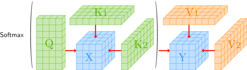
To fundamentally solve the above obstacle elegantly, [112] and [21] introduce Tensor Attention, which is a high-order attention. It is a multi-view generalization of matrix attention, i.e., $\mathsf{softmax}(Q_{A}(K_{B}\oslash K_{C})^{\top})(V_{B}\oslash V_{C})$ (Definition 3.7), where $\oslash$ is one kind of tensor operation (Definition 3.4), which can capture high-order/multi-view information intrinsically (see Figure 1). However, to implement Tensor Attention practically, we must overcome the complexity bottleneck. Let the input token length be $n$, then the forward and backward time complexity of tensor attention will be $\Omega(n^{3})$ as $Q_{A}(K_{B}\oslash K_{C})^{\top}\in\mathbb{R}^{n\times n^{2}}$ [93], while the time complexity of matrix attention is $\Omega(n^{2})$ only as $Q_{A}K_{B}^{\top}\in\mathbb{R}^{n\times n}$ [72]. For example, the input length of Llama2 [123] is 4096, so, intuitively, if we put tensor attention in Llama2, the input length will reduce to 256 to keep the same complexity in running speed and memory consumption.

There are several brilliant latest previous works to overcome the time complexity bottleneck above, e.g., $\Omega(n^{2})$ for matrix attention and $\Omega(n^{3})$ for tensor attention. [148] accelerate matrix attention forward via kernel density estimation and get truly sub-quadratic time running time. [19] uses the polynomial approximation method to map the matrix attention into low-rank matrices during forward computation, leading to an almost linear time complexity $n^{1+o(1)}$ when entries are bounded. Similarly, under sparsity assumptions, [56] achieves nearly linear time computation for matrix attention forward by identifying the larger entries in the attention matrix. On the one hand, with fine-grained analysis, [20] proposes a new backward algorithm to compute the gradient of matrix attention in almost linear time complexity $n^{1+o(1)}$ as well, under the same bounded entry assumption. On the other hand, [21] surprisingly finds that the forward computation of tensor attention can also be achieved in almost linear time $n^{1+o(1)}$ rather than almost quadratic time $n^{2+o(1)}$, under similar assumptions as [19]. See a summary in Table 1. Thus, it is natural to ask,

Can we achieve almost linear time complexity during Tensor Attention Training?

Refer to caption
Figure 1: The visualization of tensor attention with $\mathsf{softmax}$ activation function (Definition 3.7). We give an example of input token length $n=8$, feature dimension $d=4$. Here, both $\mathsf{X},\mathsf{Y}$ are tenors in shape $d\times d\times d$. There are three input matrices for each tensor.

The answer is positive. In this work, under the same bounded entries assumption as [21], we propose a method to fast compute the backward gradient of Tensor Attention Training in almost linear time as its forward computation. Thus, our results may make the tensor attention practical, as we can get around the $\Omega(n^{3})$ complexity barrier both in its forward and backward computation. We summarize our contribution as below:

Our contribution:

  • Under fine-grained analysis, we give the closed-form solution of the gradient computation of tensor attention (Lemma 4.1) and its time complexity without acceleration (Theorem 4.3).

  • Based on the closed-form solution, by utilizing polynomial approximation methods and tensor computation tricks, we propose a method to fast compute the backward gradient of tensor attention training in almost linear time as its forward computation (Theorem 5.2).

  • Furthermore, we prove that our assumption is necessary and “tight” by hardness analysis, i.e., if we slightly weaken the assumption, there is no algorithm that can solve the tensor attention gradient computation in truly sub-cubic complexity (Theorem 6.3).

2 Related Work

Large language models and transformer.

The foundation of the success of generative large language models (LLMs) lies in the decoder-only transformer architecture, as introduced by [128]. This architecture has become critical for many leading models in natural language processing (NLP) [40]. These models have already demonstrated their capabilities in various real-world applications, including language translation [59], sentiment analysis [126], and language modeling [89], due to their emergent ability, e.g., compositional ability [44, 137, 52], in-context learning [94, 88, 118]. The transformer leverages a self-attention mechanism, which enables the model to identify long-range dependencies within the input sequence. Self-attention calculates a weighted sum of input tokens, with weights based on the similarity between token pairs. This allows the model to focus on pertinent information from various parts of the sequence during output generation.

Fast attention computation.

In recent years, significant advances have been made in the development of efficient attention computation. One research direction involves employing low-rank approximations, polynomial kernel, or random features for the attention matrix [103, 78, 134, 32, 33, 151, 1, 19, 68, 110, 5], which scales the computational complexity linearly with sequence length. Another method explores patterns of sparse attention that lessen the computational load [31, 30, 147, 108, 56, 53]. Additionally, using linear attention as an alternative to softmax attention has emerged as a substantial area of study [120, 71, 114, 146, 109, 5, 118, 143, 51, 45]. These innovations have enhanced the capability of transformer-based models to handle longer sequences, thereby broadening their potential applications across various fields [37, 105, 99, 46, 92, 138, 14, 22, 62].

Tensor computation for high-order representation.

Tensors excel over matrices in capturing higher-order relationships within data. Calculating low-rank factorizations or approximations of tensors is essential in a wide range of computer science applications, such as natural language processing [38, 85, 86, 29], computer vision [129, 131, 111, 58, 55, 9, 98, 75, 34], computer graphics [130, 135, 127], security [4, 7, 67], cryptography [47, 107, 113, 73], computational biology [39, 106], and data mining [66, 102, 69, 90]. Moreover, tensors are crucial in numerous machine learning applications [91, 10, 97, 63, 57, 17, 3, 11, 12, 26, 49, 64, 16, 13, 150, 142, 115] and other diverse fields [104, 132, 42, 35, 36, 140, 116, 82, 96, 145, 141, 101].

Roadmap.

In Section 3, we introduce the notations we use, several useful definitions and our loss function. In Section 4, we give the closed form of the gradient of our loss function, and also its computational time complexity. In Section 5, we prove that we can compute the gradient in almost linear time. In Section 6, we analyze the hardness of our algorithm. In Section 7, we give the conclusion of our paper.

3 Preliminary

In this section, we first provide the notations we use. In Section 3.1, we provide general definitions related to tensor operation. In Section 3.2, we provide key definitions that we will utilize in this paper.

Refer to caption
Figure 2: The visualization of vectorization operator $\operatorname{vec}(\cdot)$, which stacks rows of a matrix $A\in\mathbb{R}^{n\times d}$ into a column vector $a\in\mathbb{R}^{nd}$. In this figure, we give an example of $n=3,d=4$. The components of $A$ and $a$ are also given for easier understanding.

Basic notations.

We use $[n]$ to denote $\{1,2,\dots,n\}$. We use $e_{i}$ to denote a column vector where only $i$-th location is $1$ and zeros everywhere else. We denote an all $1$ vector using ${\bf 1}_{n}\in\mathbb{R}^{n}$ . We use $\langle a,b\rangle$ to denote the inner product of $a,b\in\mathbb{R}^{d}$ i.e. $\langle a,b\rangle:=\sum_{i=1}^{d}a_{i}b_{i}$. We use $\|x\|_{p}$ to denote the $\ell_{p}$ norm of a vector $x\in\mathbb{R}^{n}$, i.e. $\|x\|_{2}:=(\sum_{i=1}^{n}x_{i}^{2})^{1/2}$, and $\|x\|_{\infty}:=\max_{i\in[n]}|x_{i}|$. We use $\operatorname{tr}[A]:=\sum_{i=1}^{n}A_{i,i}$ to denote the trace of a matrix $A\in\mathbb{R}^{n\times n}$. We use $\exp(A)$ to denote a matrix where $\exp(A)_{i,j}:=\exp(A_{i,j})$ for a matrix $A\in\mathbb{R}^{n\times d}$. We use $\|A\|_{\infty}$ to denote the $\ell_{\infty}$ norm of a matrix $A\in\mathbb{R}^{n\times d}$, i.e. $\|A\|_{\infty}:=\max_{i\in[n],j\in[d]}|A_{i,j}|$. We use $\|A\|_{F}$ to denote the Frobenius norm of a matrix $A\in\mathbb{R}^{n\times d}$, i.e. $\|A\|_{F}:=\sqrt{\sum_{i\in[n]}\sum_{j\in[d]}|A_{i,j}|^{2}}$. We use $\operatorname{poly}(n)$ to denote polynomial time complexity w.r.t $n$.

Tensor related notations.
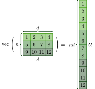
Let $A\in\mathbb{R}^{n\times d}$. We use $a:=\operatorname{vec}(A)$ to denote a length $nd$ vector. We stack rows of $A$ into a column vector, i.e. $\operatorname{vec}(A):=[a_{1}^{\top},a_{2}^{\top},\dots,a_{n}^{\top}]^{\top}$ where $a_{i}^{\top}$ is the $i$-th row of $A$, or simply $\operatorname{vec}(A)_{j+(i-1)d}:=A_{i,j}$ for any $i\in[n],j\in[d]$. Let $\mathsf{A}\in\mathbb{R}^{d_{1}\times d_{2}\times d_{3}}$ be a tensor. We use $A:=\mathrm{mat}(\mathsf{A})$ to denote a $d_{1}\times(d_{2}\cdot d_{3})$ size matrix. $\mathsf{A}_{a,b,c}=A_{a,(b-1)d_{3}+c}$ for any $a\in[d_{1}],b\in[d_{2}],c\in[d_{3}]$. Let $I_{d}\in\mathbb{R}^{d\times d}$ denote an identity matrix. Let $\mathsf{I}_{d}\in\mathbb{R}^{d\times d\times d}$ denote an identity tensor, i.e., the diagonal entries are $1$ and zeros everywhere else. Let $X\in\mathbb{R}^{d\times d^{2}}$. Let $x\in\mathbb{R}^{d^{3}}$ denote the vectorization of $X\in\mathbb{R}^{d\times d^{2}}$. Let $\mathsf{X}\in\mathbb{R}^{d\times d\times d}$ be the tesnorization of $X\in\mathbb{R}^{d\times d^{2}}$.

3.1 Definition of Tensor Operations

Here, we define some tensor operations named Kronecker product, which is a matrix operation applied to two matrices of any size, producing a block matrix. It represents a specific type of tensor product and is different from regular matrix multiplication.

Definition 3.1.

We use $\circ$ to denote the Hadamard product i.e. the $(i,j)$-entry of $A\circ B$ is $A_{i,j}B_{i,j}$.

Fact 3.2.

For all $a,b\in\mathbb{R}^{n}$, we have $\mathrm{diag}(a)\cdot b=\mathrm{diag}(b)\cdot a=a\circ b=b\circ a$.

Definition 3.3 ($\otimes$ Kronecker product).

Given $K_{1}\in\mathbb{R}^{n_{1}\times d_{1}}$ and $K_{2}\in\mathbb{R}^{n_{2}\times d_{2}}$, for any $i_{1}\in[n_{1}],i_{2}\in[n_{2}],j_{1}\in[d_{1}],j_{2}\in[d_{2}]$, we define $K:=K_{1}\otimes K_{2}\in\mathbb{R}^{n_{1}n_{2}\times d_{1}d_{2}}$ as follows

$\displaystyle K_{i_{1}+(i_{2}-1)n_{1},j_{1}+(j_{2}-1)d_{1}}=(K_{1})_{i_{1},j_{1}}\cdot(K_{2})_{i_{2},j_{2}}.$

In this work, we will primarily use the following column-wise and row-wise versions of the Kronecker product, which are special kinds of Kronecker product.

Definition 3.4 ($\oslash$ column-wise Kronecker product).

Given matrices $K_{1}\in\mathbb{R}^{n_{1}\times d},K_{2}\in\mathbb{R}^{n_{2}\times d}$, we define matrix $K:=K_{1}\oslash K_{2}\in\mathbb{R}^{n_{1}n_{2}\times d}$ as follows

$\displaystyle K_{i_{1}+(i_{2}-1)n_{1},j}:=(K_{1})_{i_{1},j}\cdot(K_{2})_{i_{2},j},~{}~{}~{}\forall i_{1}\in[n_{1}],i_{2}\in[n_{2}],j\in[d].$
Definition 3.5 ($\ominus$ row-wise Kronecker product).

Given matrices $K_{1}\in\mathbb{R}^{n\times d_{1}},K_{2}\in\mathbb{R}^{n\times d_{2}}$, we define matrix $K:=K_{1}\ominus K_{2}\in\mathbb{R}^{n\times d_{1}d_{2}}$ as follows

$\displaystyle K_{i,j_{1}+(j_{2}-1)d_{1}}:=(K_{1})_{i,j_{1}}\cdot(K_{2})_{i,j_{2}},~{}~{}~{}\forall i\in[n],j_{1}\in[d_{1}],j_{2}\in[d_{2}].$

3.2 Key Definitions of Tensor Attention

Now, we are ready to introduce the tensor attention. First, we introduce the parameters and input for a tensor attention head.

Definition 3.6 (Input and weight matrix).

We define the input sequence as $Z\in\mathbb{R}^{n\times d}$ and the key, query, and value weight matrix as $W_{K_{1}},W_{K_{2}},W_{Q},W_{V_{1}},W_{V_{2}}\in\mathbb{R}^{d\times d}$. Then, we define the key, query, and value matrix as $K_{1}:=ZW_{K_{1}}\in\mathbb{R}^{n\times d}$, $K_{2}:=ZW_{K_{2}}\in\mathbb{R}^{n\times d}$, $Q:=ZW_{Q}\in\mathbb{R}^{n\times d}$, $V_{1}:=ZW_{V_{1}}\in\mathbb{R}^{n\times d},V_{2}:=ZW_{V_{2}}\in\mathbb{R}^{n\times d}$.

Then, based on the Kronecker product, we can define our tensor attention in the following way.

Definition 3.7 (Tensor attention, Definition 1.1 in [21]).

Given input matrices $Q,K_{1},K_{2},$ $V_{1},$ $V_{2}\in\mathbb{R}^{n\times d}$, compute the following matrix

$\displaystyle\underbrace{D^{-1}}_{n\times n}\underbrace{A}_{n\times n^{2}}\underbrace{V}_{n^{2}\times d}\in\mathbb{R}^{n\times d},$

where

  • $A\in\mathbb{R}^{n\times n^{2}}$ which is defined as $A:=\exp(QK^{\top}/d)$, where $K:=K_{1}\oslash K_{2}\in\mathbb{R}^{n^{2}\times d}$,

  • $D\in\mathbb{R}^{n\times n}$ which is defined as $D:=\operatorname{diag}(A{\bf 1}_{n^{2}})$, and

  • $V\in\mathbb{R}^{n^{2}\times d}$ which is defined as $V:=V_{1}\oslash V_{2}$.

Remark 3.8.

In Definition 3.7, on the one hand, we separate the $\mathsf{softmax}$ operation into an element-wise $\exp$ operation and a diagonal normalization matrix $D$ for a more transparent formulation. On the other hand, we change $K,V\in\mathbb{R}^{n\times d}$ in classical attention to $K_{1}\oslash K_{2},V_{1}\oslash V_{2}\in\mathbb{R}^{n^{2}\times d}$ in tensor attention, where $\oslash$ is a tensor operation defined in Definition 3.4.

Our Definition 3.7 covers both the cross-attention and self-attention setting. If $Q,K_{1},K_{2},V_{1},V_{2}$ shares the same input, then it is a tensor self-attention, which can capture high-order information. If $Q,K_{1},K_{2},V_{1},V_{2}$ has different modality input, then it is a tensor cross-attention, which can capture high-order relationships among multi-modality.

Also, note that we have $A\in\mathbb{R}^{n\times n^{2}}$ in Definition 3.7. Although $QK^{\top}$ is a low-rank matrix with rank at most $d$, $\exp(QK^{\top})$ may be a full-rank matrix in general. Thus, it is clear to see the exact forward computation of tensor attention takes $\Omega(n^{3})$ time complexity. Here, we introduce a forward tensor attention approximation task, which will help us formulate the tensor attention gradient approximation task later. Furthermore, [21] shows that they can solve this approximation task in almost linear time $n^{1+o(1)}$ (Lemma 5.1).

Definition 3.9 (Approximate Tensor Attention Computation ($\mathsf{ATAttC}(n,d,B,\epsilon)$), Definition 1.2 in [21]).

Given input matrices $Q,K_{1},K_{2},V_{1},V_{2}\in\mathbb{R}^{n\times d}$ and parameters $\epsilon,B>0$, where $\max\{\|Q\|_{\infty},$ $\|K_{1}\|_{\infty},$ $\|K_{2}\|_{\infty},\|V_{1}\|_{\infty},$ $\|V_{2}\|_{\infty}\}\leq B$. Then, our target is to output a matrix $T\in\mathbb{R}^{n\times d}$ satisfying

$\displaystyle\|\underbrace{T}_{n\times d}-\underbrace{D^{-1}}_{n\times n}\underbrace{A}_{n\times n^{2}}\underbrace{V}_{n^{2}\times d}\|_{\infty}\leq\epsilon,$

where $A,D,V$ are defined in Definition 3.7.

Refer to caption
Refer to caption
Figure 3: The visualization of loss function defined in Definition 3.10. Let $A_{1},A_{2},A_{3},A_{4},A_{5}$ and $E$ be $n\times d$ input matrices. Let $Y$ be a given matrix with size $d^{2}\times d$. The Kronecker product operator $\otimes$ is defined in Definition 3.3. We minimize matrix $X\in\mathbb{R}^{d\times d^{2}}$ in our loss function. The dimensions of all matrices are given in the figure. We first compute $\exp(A_{1}X(A_{2}\otimes A_{3})^{\top})$. Then, we can compute $D(X):=\operatorname{diag}(\exp(A_{1}X(A_{2}\otimes A_{3})^{\top}){\bf 1}_{n^{2}})$. Afterwards, we compute $D(X)^{-1}\exp(A_{1}X(A_{2}\otimes A_{3})^{\top})(A_{4}\otimes A_{5})Y-E$. Finally, we optimize $X$ to compute the minimum of its Frobenius norm with a scaling factor $0.5$.

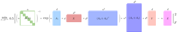
Similarly, we introduce our tensor attention optimization task. See Figure 3 for more details.

Definition 3.10 (Tensor Attention Optimization).

Suppose that $A_{1},A_{2},A_{3},A_{4},A_{5},E\in\mathbb{R}^{n\times d}$ and $Y_{1},Y_{2}\in\mathbb{R}^{d\times d}$ are given. We can formulate the attention optimization problem as

$\displaystyle\min_{X\in\mathbb{R}^{d\times d^{2}}}\mathsf{Loss}(X):=0.5\|D(X)^{-1}\exp(A_{1}X(A_{2}\otimes A_{3})^{\top}/d)(A_{4}\otimes A_{5})Y-E\|_{F}^{2},$

where

  • $A_{2}\otimes A_{3}\in\mathbb{R}^{n^{2}\times d^{2}}$ is the tensor product between $A_{2}$ and $A_{3}$

  • $D(X)=\operatorname{diag}(\exp(A_{1}XA_{2}\otimes A_{3})^{\top}/d){\bf 1}_{n^{2}})\in\mathbb{R}^{n\times n}$

  • $Y=Y_{1}\oslash Y_{2}\in\mathbb{R}^{d^{2}\times d}$

Remark 3.11.

Let weight matrices $W_{Q},W_{K_{1}},W_{K_{2}},W_{V_{1}},W_{V_{2}}\in\mathbb{R}^{d\times d}$ be defined in Definition 3.6. For the self-attention setting, we can see $A_{1},A_{2},A_{3},A_{4},A_{5}\in\mathbb{R}^{n\times d}$ as $Z\in\mathbb{R}^{n\times d}$ in Definition 3.6, and we can see $X\in\mathbb{R}^{d\times d^{2}}$ in Definition 3.10 as $W_{Q}\cdot(W_{K_{1}}\oslash W_{K_{2}})^{\top}\in\mathbb{R}^{d\times d}$ and see $Y\in\mathbb{R}^{d^{2}\times d}$ as $W_{V_{1}}\oslash W_{V_{2}}\in\mathbb{R}^{d^{2}\times d}$. To overcome the cubic complexity obstacle, we only need to handle the gradient computation of $W_{Q}\cdot(W_{K_{1}}\oslash W_{K_{2}})^{\top}\in\mathbb{R}^{d\times d}$, which is in non-linear function $\mathsf{softmax}$.

Although $X\in\mathbb{R}^{d\times d^{2}}$, we have the naive tensor attention gradient computation takes $\Omega(n^{3})$ time, as $A_{1}X(A_{2}\otimes A_{3})^{\top}\in\mathbb{R}^{n\times n^{2}}$. Thus, we formulate the below Approximate Tensor Attention Loss Gradient Computation task as our main focus.

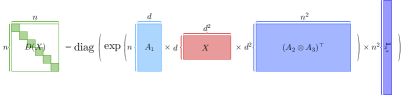
Definition 3.12 (Approximate Tensor Attention Loss Gradient Computation ($\mathsf{ATAttLGC}(n,d,B,\epsilon)$)).

Let $\epsilon,B>0$. Let $A_{1},A_{2},A_{3},A_{4},A_{5},E\in\mathbb{R}^{n\times d}$ and let $X_{1},X_{2},X_{3},Y_{1},Y_{2}\in\mathbb{R}^{d\times d}$ (see Definition 3.10). Let $X=X_{1}\cdot(X_{2}\oslash X_{3})^{\top}\in\mathbb{R}^{d\times d^{2}}$. Assume that $\max\{\|A_{1}X_{1}\|_{\infty}$, $\|A_{2}X_{2}\|_{\infty}$, $\|A_{3}X_{3}\|_{\infty}$, $\|A_{4}Y_{1}\|_{\infty}$, $\|A_{5}Y_{2}\|_{\infty}$, $\}\leq B$. Let us assume that any numbers in the previous matrices are in the $\log(n)$ bits model. We define $\mathsf{Loss}(X)$ the same as Definition 3.10. Let the gradient of loss function $\mathsf{Loss}(X)$ be $\frac{\mathrm{d}\mathsf{Loss}(X)}{\mathrm{d}X}\in\mathbb{R}^{d\times d^{2}}$. Then, our target is to output a matrix $\widetilde{g}\in\mathbb{R}^{d\times d^{2}}$ satisfying

$\displaystyle\|\widetilde{g}-\frac{\mathrm{d}\mathsf{Loss}(X)}{\mathrm{d}X}\|_{\infty}\leq\epsilon.$

4 Exact Tensor Attention Gradient Computation and Complexity

In this section, we provide the closed form of the tensor attention gradient of the loss function (Definition 3.10) and also its computational time. First, we can calculate the closed form of the gradient in the following lemma, whose proof is in Appendix E.5.

Lemma 4.1 (Close form of gradient, informal version of Lemma E.6).

Define the function $\mathsf{F}(x)\in\mathbb{R}^{n\times n^{2}}$ as in Definition D.6. Suppose that $A_{1},A_{2},A_{3}\in\mathbb{R}^{n\times d}$ are three given matrices. Suppose that $\mathsf{Loss}(x)$ is defined as Definition 3.10, where $x=\operatorname{vec}(X)$. Then, we can show

$\displaystyle\frac{\mathrm{d}\mathsf{Loss}(x)}{\mathrm{d}x}=\operatorname{vec}(A_{1}^{\top}\mathsf{F}(x)(A_{2}\otimes A_{3}))\in\mathbb{R}^{d^{3}}.$

Note that, $\mathsf{F}(x)$ is a size $n\times n^{2}$ matrix which is the bottleneck obstacle in time complexity.

Definition 4.2.

Let ${\cal T}_{\mathrm{mat}}(a,b,c)$ denote the time of multiplying $a\times b$ matrix and $b\times c$ matrix.

Then, with straightforward analysis, we get the following theorem about the time complexity of naive computation. The complete proof is in Appendix E.6.

Theorem 4.3 (Tensor attention gradient computation, informal version of Theorem E.7).

Suppose that $A_{1},A_{2},A_{3},$ $A_{4},A_{5},E\in\mathbb{R}^{n\times d}$ are input fixed matrices. We denote matrix variables as $X\in\mathbb{R}^{d\times d^{2}}$ and $Y\in\mathbb{R}^{d^{2}\times d}$ (gradient computation is w.r.t. $X$ ). Let $g=\frac{\mathrm{d}\mathsf{Loss}(X)}{\mathrm{d}X}\in\mathbb{R}^{d\times d^{2}}$ (for definition of $\mathsf{Loss}(X)$, see Definition 3.10). Then we can demonstrate that computing the gradient $g\in\mathbb{R}^{d\times d^{2}}$ requires ${\cal T}_{\mathrm{mat}}(n,d^{2},n^{2})$ time.

Note that ${\cal T}_{\mathrm{mat}}(n,d^{2},n^{2})\geq\Omega(n^{3})$. Thus, the naive tensor attention gradient computation is a complexity obstacle in practice as discussed in Section 1. Based on the closed formulation in Lemma 4.1, we will have our acceleration method, which will be introduced in the following section.

5 Fast Gradient Computation via Tensor Trick and Polynomial Method

In this section, we show how to compute the tensor attention matrix gradient in almost linear time. In Section 5.1, we demonstrate our main results. In Section 5.2, we introduce some key tensor tricks that are used in our proof.

5.1 Main Results for Fast Gradient Computation

Polynomial approximation methods involve representing complex functions through simpler polynomial forms to facilitate easier analysis and computation. They are crucial in numerical analysis, aiding in the efficient solution of differential equations and optimization problems, and are widely used in simulations and machine learning [1, 6].

Based on the polynomial approximation methods, [21] get the following lemma about tensor attention acceleration, which will be used in our main results proof.

Lemma 5.1 (Theorem 1.4 in [21]).

There is an algorithm that solves $\mathsf{ATAttC}(n,d=O(\log n),B=o(\sqrt[3]{\log n}),\epsilon=1/\operatorname{poly}(n))$ (see Definition 3.9) in time $n^{1+o(1)}$.

Using similar polynomial approximation methods, with many more tensor analysis techniques (Section 5.2), we can get our main acceleration results.

Theorem 5.2 (Main result for fast gradient computation).

Assuming the entries of $A_{1},A_{2},$ $A_{3},$ $A_{4},A_{5},E\in\mathbb{R}^{n\times d}$ and $X_{1},X_{2},X_{3},Y_{1},Y_{2}\in\mathbb{R}^{d\times d}$ are represented using $O(\log n)$ bits. Then, there exist an algorithm that runs in $n^{1+o(1)}$ time to solve $\mathsf{ATAttLGC}(n,d=O(\log n),B=o(\sqrt[3]{\log n}),\epsilon=1/\operatorname{poly}(n))$ (see Definition 3.12), i.e., our algorithm computes a gradient matrix $\widetilde{g}\in\mathbb{R}^{d\times d^{2}}$ satisfying $\|\frac{\mathrm{d}\mathsf{Loss}(X)}{\mathrm{d}X}-\widetilde{g}\|_{\infty}\leq 1/\operatorname{poly}(n)$.

Proof sketch of Theorem 5.2.

The complete proof can be found in Appendix F.6.

We can use the polynomial approximation method to get low-rank approximation results for $D^{-1}\exp(A_{1}X(A_{2}\otimes A_{3})^{\top}/d)$ in Lemma F.1. Then, based on the close form of the tensor attention gradient solution in Theorem 4.3 and many tensor tricks (Section 5.2 and Appendix C), we can smartly convey these low rank properties to the gradient formulation, where two key steps need to be fixed (see details in Lemma F.5 and Lemma F.7). ∎

Remark 5.3.

The assumption in Theorem 5.2 is practical. In practice, the $n$ is super large, e.g, $n=2,000,000$ for Google’s Gemini 1.5 Pro  [48], while the model training uses a half-precision floating-point format, e.g., the bit number is a constant $16$. On the other hand, our assumption is “tight”, where if we slightly weaken the assumption, there is no algorithm that can solve the tensor attention gradient computation in truly sub-cubic complexity (Theorem 6.3).

Our Theorem 5.2 can accurately approximate ($\epsilon=1/\operatorname{poly}(n)$) the tensor attention gradient computation in almost linear time $n^{1+o(1)}$ under practical assumptions (see discussion in Remark 5.3). Thus, our methods solve the last puzzle of tensor attention acceleration. This may make tensor attention practical, as we can get around the cubic time complexity barrier both in inference and training.

5.2 Tensor Operation Analysis Techniques

Here, we introduce some key techniques during proof Theorem 5.2. These techniques make it possible to convey the low-rank property even during the tensor computation.

We first introduce a swap rule and a distributed rule, where both proofs are in Appendix C.2

Fact 5.4 (Swap rule for tensor product and matrix product).

Let $W_{1},W_{2}\in\mathbb{R}^{d\times d}$ and $A_{1},A_{2}\in\mathbb{R}^{n\times d}$. We have

$\displaystyle\underbrace{(A_{1}\otimes A_{2})}_{{n^{2}\times d^{2}}}\cdot\underbrace{(W_{1}\oslash W_{2})}_{{d^{2}\times d}}=\underbrace{(A_{1}\cdot W_{1})}_{{n\times d}}\oslash\underbrace{(A_{2}\cdot W_{2})}_{{n\times d}}.$

Fact 5.4 tells us that we can swap the order of tensor operation and matrix multiplication, so we can always compute the low dimension first to reduce the complexity.

Fact 5.5.

Let $U_{1}\in\mathbb{R}^{n_{1}\times d}$ and $U_{2}\in\mathbb{R}^{n_{1}\times k}$. Let $V_{1}\in\mathbb{R}^{n_{2}\times d}$ and $V_{2}\in\mathbb{R}^{n_{2}\times k}$. Let $W_{1}\in\mathbb{R}^{n_{3}\times d}$ and $W_{2}\in\mathbb{R}^{n_{3}\times k}$. We have

$\displaystyle\underbrace{(U_{1}\ominus U_{2})}_{n_{1}\times dk}\cdot(\underbrace{(V_{1}\ominus V_{2})}_{n_{2}\times dk}\oslash\underbrace{(W_{1}\ominus W_{2})}_{n_{3}\times dk})^{\top}=(\underbrace{U_{1}}_{n_{1}\times d}(\underbrace{V_{1}}_{n_{2}\times d}\oslash\underbrace{W_{1}}_{n_{3}\times d})^{\top})\circ(\underbrace{U_{2}}_{n_{1}\times k}(\underbrace{V_{2}}_{n_{2}\times k}\oslash\underbrace{W_{2}}_{n_{3}\times k})^{\top})$

Fact 5.5 tells us that the multiple tensor operation can be distributed to a different format. If we have some low-rank matrix/tensor, we can distribute them to each component so that each component can be accelerated. The high-level intuition sounds like we borrow some benefits from other terms to fix the bottleneck term.

We prove an important tool whose proof is in Appendix C.2.

Lemma 5.6 ( Informal version of Lemma C.14 ).

Given $A_{1}\in\mathbb{R}^{n_{1}\times d_{1}}$, $A_{2}\in\mathbb{R}^{n_{2}\times d_{1}}$, let $A:=(A_{1}\oslash A_{2})\in\mathbb{R}^{n_{1}n_{2}\times d_{1}}$. Given $B_{1}\in\mathbb{R}^{n_{1}\times d_{2}}$, $B_{2}\in\mathbb{R}^{n_{2}\times d_{2}}$, let $B:=(B_{1}\oslash B_{2})\in\mathbb{R}^{n_{1}n_{2}\times d_{2}}$. We define $C\in\mathbb{R}^{d_{1}\times d_{2}}$ as $C:=A^{\top}B$ and $C_{1}:=A_{1}^{\top}B_{1}\in\mathbb{R}^{d_{1}\times d_{2}},C_{2}:=A_{2}^{\top}B_{2}\in\mathbb{R}^{d_{1}\times d_{2}}$. Then, we have

  • Part 1. $C_{1}\circ C_{2}=C$

  • Part 2. Given $A_{1},A_{2},B_{1},B_{2}$, we can get $C$ in ${\cal T}_{\mathrm{mat}}(d_{1},\max\{n_{1},n_{2}\},d_{2})$ time.

Lemma C.14 is a highly non-trivial method to handle tensor operation, $\circ$ and matrix multiplication together. By using the method, we can save the computation time from ${\cal T}_{\mathrm{mat}}(d,n^{2},d)$ to ${\cal T}_{\mathrm{mat}}(d,n,d)$, which gets rid of the bottleneck quadratic term $n^{2}$.

Lastly, we introduce a tensor trick, which can reduce a tensor operation to a matrix multiplication operation. The proof is in Appendix C.3.

Fact 5.7 (Tensor-trick).

Given matrices $A_{1}\in\mathbb{R}^{n_{1}\times d_{1}},A_{2}\in\mathbb{R}^{n_{2}\times d_{2}}$ and $X\in\mathbb{R}^{d_{1}\times d_{2}}$, we have $\operatorname{vec}(A_{1}XA_{2}^{\top})=(A_{1}\otimes A_{2})\operatorname{vec}(X)\in\mathbb{R}^{n_{1}n_{2}}$.

6 Tensor Attention Gradient Computation Complexity Lower Bound

In this section, we will show that our assumption is “tight”. First, we introduce some hardness analysis background in Section 6.1. Then, we will introduce our main hardness result in Section 6.2.

6.1 Strong Exponential Time Hypothesis and Tensor Attention Forward Hardness

We provide the findings that our results are based on. We first introduce a well-known hypothesis. The Strong Exponential Time Hypothesis ($\mathsf{SETH}$), a well-established conjecture, has been instrumental in establishing fine-grained lower bounds for numerous algorithmic problems, as highlighted in the survey by [133]. More than two decades ago, [61] introduced $\mathsf{SETH}$ as an enhanced version of the $\mathsf{P}\neq\mathsf{NP}$ conjecture, positing that current solving $\mathsf{SAT}$ problem algorithms are nearly optimal in terms of efficiency.

Hypothesis 6.1 (Strong Exponential Time Hypothesis ($\mathsf{SETH}$), [61]).

Given $\epsilon>0$, there exists $k\geq 3\in\operatorname*{\mathbb{Z}}$ such that it is impossible to solve $k$-$\mathsf{SAT}$ problem with $n$ variables in $O(2^{(1-\epsilon)n})$ time, including using any randomized algorithms.

We will critically utilize the hardness result of the forward tensor attention computation from previous work as follows.

Lemma 6.2 (Theorem 1.3 in [21]).

Assuming $\mathsf{SETH}$, for any constant $\delta>0$, no algorithm can solve $\mathsf{ATAttC}(n,d=\Theta(\log n),B=\Theta(\sqrt[3]{(1+\gamma)\log n}),\epsilon=n^{\gamma-O(1)})$ (Definition 3.9) in $O(n^{3-\delta})$ time, even if the inputs meet the following conditions for any $\gamma\geq 0$: (1) $V\in\{0,1\}^{n^{2}\times d}$, (2) There exists $B_{a}\leq O((1+\gamma)\log^{2}n)=O(d(\sqrt[3]{(1+\gamma)\log n})^{3})$ where all entries of $QK^{\top}$ are within the range $[1,B_{a}]$ and more than half entries in each row of $QK^{\top}$ are equal to $B_{a}$.

If we change the assumption from $B=O(\sqrt[3]{\log n})$ to $B=\Theta(\sqrt[3]{(1+\gamma)\log n}$ with $\gamma=\omega(1)$, Lemma 6.2 shows that tenor attention forward computation is hard, i.e., no algorithm can solve it in truly sub-cubic time (assume $\mathsf{SETH}$).

6.2 Main Results for Hardness

Based on the above observation (Lemma 6.2), we can prove our main results for tensor attention gradient computation hardness.

Theorem 6.3 (Main result for hardness).

Let $\gamma:\mathbb{N}\to\mathbb{N}$ be any function with $\gamma(n)=o(\log n)$ and $\gamma(n)=\omega(1)$. Assuming $\mathsf{SETH}$, for any constant $\delta>0$, it is impossible to solve $\mathsf{ATAttLGC}(n,d=\Theta(\log n),B=\Theta(\sqrt[3]{\gamma(n)\cdot\log n}),\epsilon=O(1/(\log n)^{4}))$ (Definition 3.12) in time $O(n^{{{}{}{}3}-\delta})$ when $E=0$, $\mathsf{Y}=\mathsf{I}_{d}$, $\mathsf{X}=\lambda\mathsf{I}_{d}$ for some scalar $\lambda\in[0,1]$.

See the formal proof in Appendix G.2. The intuition is that if we can solve $\mathsf{ATAttLGC}$ in $O(t)$ time, then we can solve $\mathsf{ATAttC}$ in $O(t\cdot\log^{11}(n))$ time by interpolation and “integral”.

We see a similar sharp complexity transition as forward computation (Lemma 6.2), when we change the assumption from $B=O(\sqrt[3]{\log n})$ to $B=\Theta(\sqrt[3]{(1+\gamma)\log n})$ with $\gamma=\omega(1)$, where the tensor attention gradient computation will be unsolvable in truly sub-cubic time as well (assume $\mathsf{SETH}$).

7 Conclusion

In this work, we prove that the backward gradient of tensor attention training can be computed in almost linear $n^{1+o(1)}$ time, the same complexity as its forward computation, under a bounded entries assumption. We provide a closed-form solution for the gradient and propose a fast computation method utilizing polynomial approximation techniques and tensor algebraic tricks. Furthermore, we prove the necessity and tightness of our assumption through hardness analysis, showing that slightly weakening it renders the gradient problem unsolvable in truly subcubic time. Our theoretical results establish the feasibility of efficient higher-order transformer training and may facilitate practical applications of tensor attention architectures. Future work can explore how these findings can be implemented in real-world scenarios to enable the development of powerful multi-modality models.

Acknowledgement

Research is partially supported by the National Science Foundation (NSF) Grants 2023239-DMS, CCF-2046710, and Air Force Grant FA9550-18-1-0166.

Appendix

Roadmap.

In Section A, we provide the potential limitations of this work. In Section B, we discuss the societal impacts of our work. In Section C, we provide general definitions and several basic facts. In Section D, we show how we calculate the gradient of the loss function defined by Definition 3.10. In Section E, we show the time complexity of our algorithm. In Section F, we show that our algorithm can be computed in polynomial time. In Section G, we show the hardness of our algorithm.

Appendix A Limitations

This work has not directly addressed the practical applications of our results, as we have not implemented our tensor attention algorithm. Future research could investigate how these findings could be applied in real-world scenarios.

Appendix B Societal Impacts

We delve into and offer a deeper understanding of the attention mechanism, introducing a novel approach to integrate multi-modality into attention through the tensor attention algorithm. We also demonstrate that the computation of both forward and backward tensor attention can be achieved with almost linear time complexity.

Regarding the negative societal impact, since our work is completely theoretical in nature, we do not foresee any potential negative societal impacts which worth pointing out.

Appendix C Tensor Operation Background

In Section C.1, we define the notation of computational time and the tensor operation. In Section C.2, we provide some helpful facts of tensor operation. In Section C.3, we provide some helpful facts of vectorization operation.

C.1 General definitions and tensor operation

Fact C.1 ([25, 27]).

We can show that ${\cal T}_{\mathrm{mat}}(a,b,c)=O({\cal T}_{\mathrm{mat}}(a,c,b))=O({\cal T}_{\mathrm{mat}}(b,a,c))=O({\cal T}_{\mathrm{mat}}(b,c,a))=O({\cal T}_{\mathrm{mat}}(c,a,b))=O({\cal T}_{\mathrm{mat}}(c,b,a))$.

Definition C.2 ($\odot$ tensor computation).

Given matrices $A\in\mathbb{R}^{n\times d}$, $B\in\mathbb{R}^{n\times d}$, $C\in\mathbb{R}^{n\times d}$, we use $T=A\odot B\odot C\in\mathbb{R}^{n\times n\times n}$ to denote an tensor whose entries are given by

$\displaystyle T_{i,j,l}:=\sum_{a=1}^{d}A_{i,a}B_{j,a}C_{l,a},~{}~{}~{}\forall i\in[n],j\in[n],l\in[n].$

We note that a tensor $T$ can be written in the form $A\odot B\odot C$ like this if and only if its tensor rank is at most $d$.

Definition C.3 ($(\cdot,\cdot,\cdot)$).

Let $\mathsf{X}\in\mathbb{R}^{d\times d\times d}$. Given matrices $A_{1}\in\mathbb{R}^{n\times d}$, $A_{2}\in\mathbb{R}^{n\times d}$ and $A_{3}\in\mathbb{R}^{n\times d}$.

Let operator $\mathsf{X}(A_{1},A_{2},A_{3})\in\mathbb{R}^{n\times n\times n}$ satisfying

$\displaystyle\mathsf{X}(A_{1},A_{2},A_{3})_{i,j,l}:=\sum_{a=1}^{d}\sum_{b=1}^{d}\sum_{c=1}^{d}\mathsf{X}_{a,b,c}(A_{1})_{i,a}(A_{2})_{j,b}(A_{3})_{l,c},~{}~{}~{}~{}\forall i\in[n],j\in[n],l\in[n]$

C.2 Facts for tensor operation

Fact C.4.

We can show two results

  • Suppose that $\underbrace{K}_{n_{1}n_{2}\times d}=\underbrace{K_{1}}_{n_{1}\times d}\oslash\underbrace{K_{2}}_{n_{2}\times d}$. We have $\underbrace{K^{\top}}_{d\times n_{1}n_{2}}=\underbrace{K_{1}^{\top}}_{d\times n_{1}}\ominus\underbrace{K_{2}^{\top}}_{d\times n_{2}}$.

  • Suppose that $\underbrace{Q}_{n\times d_{1}d_{2}}=\underbrace{Q_{1}}_{n\times d_{1}}\ominus\underbrace{Q_{2}}_{n\times d_{2}}$. We have $\underbrace{Q^{\top}}_{d_{1}d_{2}\times n}=\underbrace{Q_{1}^{\top}}_{d_{1}\times n}\oslash\underbrace{Q_{2}^{\top}}_{d_{2}\times n}$.

  • Suppose that $\underbrace{V}_{n_{1}n_{2}\times d_{1}d_{2}}=\underbrace{V_{1}}_{n_{1}\times d_{1}}\otimes\underbrace{V_{2}}_{n_{2}\times d_{2}}$. We have $\underbrace{V^{\top}}_{d_{1}d_{2}\times n_{1}n_{2}}=\underbrace{V_{1}^{\top}}_{d_{1}\times n_{1}}\otimes\underbrace{V_{2}^{\top}}_{d_{2}\times n_{2}}$.

Proof.

The proof is very straightforward. ∎

Fact C.5 (Swap rule).

Let $V_{1}\in\mathbb{R}^{n\times d}$. Let $V_{2}\in\mathbb{R}^{n\times k}$. Let $W_{1}\in\mathbb{R}^{m\times d}$. Let $W_{2}\in\mathbb{R}^{m\times k}$. We can show swap rule for $\oslash$ and $\ominus$,

$\displaystyle\underbrace{(V_{1}\ominus V_{2})}_{n\times dk}\oslash\underbrace{(W_{1}\ominus W_{2})}_{m\times dk}=\underbrace{(V_{1}\oslash W_{1})}_{mn\times d}\ominus\underbrace{(V_{2}\oslash W_{2})}_{mn\times k}$

And we can show swap rule for $\otimes$ and $\ominus$,

$\displaystyle\underbrace{(V_{1}\ominus V_{2})}_{n\times dk}\otimes\underbrace{(W_{1}\ominus W_{2})}_{m\times dk}=\underbrace{(V_{1}\otimes W_{1})}_{mn\times dk}\ominus\underbrace{(V_{2}\otimes W_{2})}_{mn\times dk}$
Proof.

The proof is trivially following from definition of $\oslash$ and $\ominus$.

Note that for any $i_{1}\in[n],i_{2}\in[m],j_{1}\in[d],j_{2}\in[k]$

$\displaystyle~{}((V_{1}\ominus V_{2})\oslash(W_{1}\ominus W_{2}))_{i_{1}+(i_{2}-1)n,j_{1}+(j_{2}-1)d}$
$\displaystyle=$ $\displaystyle~{}(V_{1})_{i_{1},j_{1}}(V_{2})_{i_{1},j_{2}}(W_{1})_{i_{2},j_{1}}(W_{2})_{i_{2},j_{2}}$
$\displaystyle=$ $\displaystyle~{}((V_{1}\oslash W_{1})\ominus(V_{2}\oslash W_{2}))_{i_{1}+(i_{2}-1)n,j_{1}+(j_{2}-1)d}$

Thus, we complete the proof. ∎

Remark C.6.

In Fact C.5, due to definition $V_{1}$ and $V_{2}$ need to have the same number of rows. $W_{1}$ and $W_{2}$ also need to have the same number of rows. $V_{1}$ and $W_{1}$ need to have same number of columns, and $V_{2}$ and $V_{2}$ need to have same number of columns.

Fact C.7 (Swap rule for tensor product and matrix product, Restatement of Fact 5.4).

Let $W_{1},W_{2}\in\mathbb{R}^{d\times d}$ and $A_{1},A_{2}\in\mathbb{R}^{n\times d}$. We have

$\displaystyle\underbrace{(A_{1}\otimes A_{2})}_{{n^{2}\times d^{2}}}\cdot\underbrace{(W_{1}\oslash W_{2})}_{{d^{2}\times d}}=\underbrace{(A_{1}\cdot W_{1})}_{{n\times d}}\oslash\underbrace{(A_{2}\cdot W_{2})}_{{n\times d}}.$
Proof of Fact 5.4.

For any $i_{1},i_{2}\in[n],j\in[d]$, we have

$\displaystyle~{}((A_{1}\otimes A_{2})\cdot(W_{1}\oslash W_{2}))_{i_{1}+(i_{2}-1)n,j}$
$\displaystyle=$ $\displaystyle~{}\sum_{k_{1}\in[d],k_{2}\in[d]}(A_{1}\otimes A_{2})_{i_{1}+(i_{2}-1)n,k_{1}+(k_{2}-1)d}(W_{1}\oslash W_{2})_{k_{1}+(k_{2}-1)d,j}$
$\displaystyle=$ $\displaystyle~{}\sum_{k_{1}\in[d],k_{2}\in[d]}(A_{1}\otimes A_{2})_{i_{1}+(i_{2}-1)n,k_{1}+(k_{2}-1)d}\cdot(W_{1})_{k_{1},j}\cdot(W_{2})_{k_{2},j}$
$\displaystyle=$ $\displaystyle~{}\sum_{k_{1}\in[d],k_{2}\in[d]}(A_{1})_{i_{1},k_{1}}\cdot(A_{2})_{i_{2},k_{2}}\cdot(W_{1})_{k_{1},j}\cdot(W_{2})_{k_{2},j}$
$\displaystyle=$ $\displaystyle~{}(\sum_{k_{1}\in[d]}(A_{1})_{i_{1},k_{1}}\cdot(W_{1})_{k_{1},j})\cdot(\sum_{k_{2}\in[d]}(A_{2})_{i_{2},k_{2}}\cdot(W_{2})_{k_{2},j})$
$\displaystyle=$ $\displaystyle~{}(A_{1}\cdot W_{1})_{i_{1},j}\cdot(A_{2}\cdot W_{2})_{i_{2},j}$
$\displaystyle=$ $\displaystyle~{}((A_{1}\cdot W_{1})\oslash(A_{2}\cdot W_{2}))_{i_{1}+(i_{2}-1)n,j},$

where the first step follows matrix multiplication, the second step follows Definition 3.4, the third step follows Definition 3.3, the fourth step follows simple algebra, the fifth step follows matrix multiplication and the last step follows Definition 3.4. ∎

Fact C.8.

Let $X=\underbrace{\mathrm{mat}(\mathsf{I}_{d})}_{d\times d^{2}}$, where $\mathsf{I}_{d}\in\mathbb{R}^{d\times d\times d}$ and $A_{1},A_{2}\in\mathbb{R}^{n\times d}$. We have

$\displaystyle\underbrace{(A_{1}\otimes A_{2})}_{{n^{2}\times d^{2}}}\underbrace{X^{\top}}_{{d^{2}\times d}}=\underbrace{A_{1}\oslash A_{2}}_{{n^{2}\times d}}$
Proof.

For any $i_{1},i_{2}\in[n],j\in[d]$, we have

$\displaystyle((A_{1}\otimes A_{2})X^{\top})_{i_{1}+(i_{2}-1)n,j}=$ $\displaystyle~{}\sum_{k_{1}\in[d],k_{2}\in[d]}(A_{1}\otimes A_{2})_{i_{1}+(i_{2}-1)n,k_{1}+(k_{2}-1)d}X_{j,k_{1}+(k_{2}-1)d}$
$\displaystyle=$ $\displaystyle~{}\sum_{k_{1}\in[d],k_{2}\in[d]}(A_{1})_{i_{1},k_{1}}\cdot(A_{2})_{i_{2},k_{2}}X_{j,k_{1}+(k_{2}-1)d}$
$\displaystyle=$ $\displaystyle~{}(A_{1})_{i_{1},j}\cdot(A_{2})_{i_{2},j}$
$\displaystyle=$ $\displaystyle~{}(A_{1}\oslash A_{2})_{i_{1}+(i_{2}-1)n,j},$

where the first step is due to matrix multiplication, the second step follows Definition 3.3, the third step follows $X_{j,k_{1}+(k_{2}-1)d}=1$ when $j=k_{1}=k_{2}$, and $X_{j,k_{1}+(k_{2}-1)d}=0$ otherwise, and the last step is because of Definition 3.4. ∎

Fact C.9 (Restatement of Fact 5.5).

Let $U_{1}\in\mathbb{R}^{n_{1}\times d}$ and $U_{2}\in\mathbb{R}^{n_{1}\times k}$. Let $V_{1}\in\mathbb{R}^{n_{2}\times d}$ and $V_{2}\in\mathbb{R}^{n_{2}\times k}$. Let $W_{1}\in\mathbb{R}^{n_{3}\times d}$ and $W_{2}\in\mathbb{R}^{n_{3}\times k}$. We have

$\displaystyle\underbrace{(U_{1}\ominus U_{2})}_{n_{1}\times dk}\cdot(\underbrace{(V_{1}\ominus V_{2})}_{n_{2}\times dk}\oslash\underbrace{(W_{1}\ominus W_{2})}_{n_{3}\times dk})^{\top}=(\underbrace{U_{1}}_{n_{1}\times d}(\underbrace{V_{1}}_{n_{2}\times d}\oslash\underbrace{W_{1}}_{n_{3}\times d})^{\top})\circ(\underbrace{U_{2}}_{n_{1}\times k}(\underbrace{V_{2}}_{n_{2}\times k}\oslash\underbrace{W_{2}}_{n_{3}\times k})^{\top})$
Proof of Fact 5.5.

We can show that

$\displaystyle(U_{1}\ominus U_{2})((V_{1}\ominus V_{2})\oslash(W_{1}\ominus W_{2}))^{\top}=$ $\displaystyle~{}(U_{1}\ominus U_{2})((V_{1}\oslash W_{1})\ominus(V_{2}\oslash W_{2}))^{\top}$
$\displaystyle=$ $\displaystyle~{}(U_{1}\ominus U_{2})((V_{1}\oslash W_{1})^{\top}\oslash(V_{2}\oslash W_{2})^{\top})$
$\displaystyle=$ $\displaystyle~{}(U_{1}^{\top}\oslash U_{2}^{\top})^{\top}((V_{1}\oslash W_{1})^{\top}\oslash(V_{2}\oslash W_{2})^{\top})$
$\displaystyle=$ $\displaystyle~{}(U_{1}(V_{1}\oslash W_{1})^{\top})\circ(U_{2}(V_{2}\oslash W_{2})^{\top})$

where first step is due to swapping rule for $\oslash$ and $\ominus$ (see Fact C.5), the second step follows from Fact C.4, the third step follows from Fact C.4, and the last step follows from Lemma C.14. ∎

Fact C.10.

Let $U_{1}\in\mathbb{R}^{n_{1}\times d^{2}}$ and $U_{2}\in\mathbb{R}^{n_{1}\times k^{2}}$. Let $V_{1}\in\mathbb{R}^{n_{2}\times d}$ and $V_{2}\in\mathbb{R}^{n_{2}\times k}$. Let $W_{1}\in\mathbb{R}^{n_{3}\times d}$ and $W_{2}\in\mathbb{R}^{n_{3}\times k}$. We have

$\displaystyle\underbrace{(U_{1}\ominus U_{2})}_{n_{1}\times d^{2}k^{2}}\cdot(\underbrace{(V_{1}\ominus V_{2})}_{n_{2}\times dk}\otimes\underbrace{(W_{1}\ominus W_{2})}_{n_{3}\times dk})^{\top}=(\underbrace{U_{1}}_{n_{1}\times d^{2}}(\underbrace{V_{1}}_{n_{2}\times d}\otimes\underbrace{W_{1}}_{n_{3}\times d})^{\top})\circ(\underbrace{U_{2}}_{n_{1}\times k^{2}}(\underbrace{V_{2}}_{n_{2}\times k}\otimes\underbrace{W_{2}}_{n_{3}\times k})^{\top})$
Proof.

We can show that,

$\displaystyle~{}\underbrace{(U_{1}\ominus U_{2})}_{n_{1}\times d^{2}k^{2}}\cdot(\underbrace{(V_{1}\ominus V_{2})}_{n_{2}\times dk}\otimes\underbrace{(W_{1}\ominus W_{2})}_{n_{3}\times dk})^{\top}$
$\displaystyle=$ $\displaystyle~{}\underbrace{(U_{1}\ominus U_{2})}_{n_{1}\times d^{2}k^{2}}\cdot((V_{1}\otimes W_{1})\ominus(V_{2}\otimes W_{2}))^{\top}$
$\displaystyle=$ $\displaystyle~{}(U_{1}\ominus U_{2})\cdot((V_{1}\otimes W_{1})^{\top}\oslash(V_{2}\otimes W_{2})^{\top})$
$\displaystyle=$ $\displaystyle~{}(U_{1}^{\top}\oslash U_{2}^{\top})^{\top}\cdot((V_{1}\otimes W_{1})^{\top}\oslash(V_{2}\otimes W_{2})^{\top})$
$\displaystyle=$ $\displaystyle~{}(\underbrace{U_{1}}_{n_{1}\times d^{2}}(\underbrace{V_{1}}_{n_{2}\times d}\otimes\underbrace{W_{1}}_{n_{3}\times d})^{\top})\circ(\underbrace{U_{2}}_{n_{1}\times k^{2}}(\underbrace{V_{2}}_{n_{2}\times k}\otimes\underbrace{W_{2}}_{n_{3}\times k})^{\top})$

where the first step is because of the swap rule for $\otimes$ and $\ominus$ (see Fact C.5), the second step follows from Fact C.4, the third step follows from Fact C.4, and the last step follows from Lemma C.14. ∎

Claim C.11.

Let $A,B,C\in\mathbb{R}^{n\times d}$.

Part 1. Let $I_{d}\in\mathbb{R}^{d\times d}$ denote an identity matrix. Then, we have

$\displaystyle AI_{d}B^{\top}=AB^{\top}.$

Part 2. Let $\mathsf{I}_{d}\in\mathbb{R}^{d\times d\times d}$ denote an identity tensor. Then we can show that

$\displaystyle\mathsf{I}_{d}(A,B,C)=A\odot B\odot C$
Proof.

Now we prove for each part.

Proof of Part1. Using the property of identity matrix, it’s easy to see this holds.

Proof of Part2.

$\displaystyle\mathsf{I}_{d}(A,B,C)=$ $\displaystyle~{}\sum_{a=1}^{d}\sum_{b=1}^{d}\sum_{c=1}^{d}(\mathsf{I}_{d})_{a,b,c}(A)_{i,a}(B)_{j,b}(C)_{l,c}$
$\displaystyle=$ $\displaystyle~{}\sum_{a=1}^{d}(A)_{i,a}(B)_{j,a}(C)_{l,a}$
$\displaystyle=$ $\displaystyle~{}A\odot B\odot C$

where the first step follows from Definition C.3, the second step follows from the property of identity tensor $(\mathsf{I}_{d})_{i,j,k}$, which equals $1$ only when $i=j=k$ and 00 elsewhere, and the last step follows from Definition C.2. ∎

Fact C.12.

Let $U,V,W\in\mathbb{R}^{n\times d}$, we have

$\displaystyle\underbrace{U(V\oslash W)^{\top}}_{{n\times n^{2}}}=\underbrace{\mathsf{mat}(U\odot V\odot W)}_{{n\times n^{2}}}.$
Proof.

For any $i,j,k\in[n]$, we have

$\displaystyle\mathsf{mat}(U\odot V\odot W)_{i,(j-1)n+k}=$ $\displaystyle~{}(U\odot V\odot W)_{i,j,k}$
$\displaystyle=$ $\displaystyle~{}\sum_{a\in[d]}U_{i,a}V_{j,a}W_{k,a}$
$\displaystyle=$ $\displaystyle~{}\sum_{a\in[d]}U_{i,a}(V\oslash W)_{(j-1)n+k,a}$
$\displaystyle=$ $\displaystyle~{}\sum_{a\in[d]}U_{i,a}((V\oslash W)^{\top})_{a,(j-1)n+k}$
$\displaystyle=$ $\displaystyle~{}(U(V\oslash W)^{\top})_{i,(j-1)n+k},$

where the first step by definition of $\mathsf{mat}$, the second step follows Definition C.2, the third step follows Definition 3.4, the fourth step follows from transpose, and the last step follows from matrix multiplication. ∎

Fact C.13.

Given $A_{1},A_{2},A_{3}\in\mathbb{R}^{n\times d}$ and $W_{1},W_{2},W_{3}\in\mathbb{R}^{n\times k}$, we have

$\displaystyle\underbrace{[W_{1}\odot W_{2}\odot W_{3}](A_{1}^{\top},A_{2}^{\top},A_{3}^{\top})}_{{d\times d\times d}}=\underbrace{((A_{1}^{\top}W_{1})\odot(A_{2}^{\top}W_{2})\odot(A_{3}^{\top}W_{3}))}_{{d\times d\times d}}.$
Proof.

The proof is trivial by Definition C.2 and Definition C.3. ∎

We prove an important tool, which will be used in analyzing the running time of our algorithm.

Lemma C.14 ( Formal version of Lemma 5.6 ).

If the following condition holds

  • Let $\oslash$ be defined as Definition 3.4.

  • Given $A_{1}\in\mathbb{R}^{n_{1}\times d_{1}}$, $A_{2}\in\mathbb{R}^{n_{2}\times d_{1}}$, let $A:=(A_{1}\oslash A_{2})\in\mathbb{R}^{n_{1}n_{2}\times d_{1}}$.

  • Given $B_{1}\in\mathbb{R}^{n_{1}\times d_{2}}$, $B_{2}\in\mathbb{R}^{n_{2}\times d_{2}}$, let $B:=(B_{1}\oslash B_{2})\in\mathbb{R}^{n_{1}n_{2}\times d_{2}}$.

  • We define $C\in\mathbb{R}^{d_{1}\times d_{2}}$ as $C:=A^{\top}B$

  • We define $\underbrace{C_{1}}_{d_{1}\times d_{2}}:=A_{1}^{\top}B_{1},\underbrace{C_{2}}_{d_{1}\times d_{2}}:=A_{2}^{\top}B_{2}$

Then, we have

  • Part 1. $C_{1}\circ C_{2}=C$

  • Part 2. Given as input $A_{1},A_{2},B_{1},B_{2}$, we can get $C$ in ${\cal T}_{\mathrm{mat}}(d_{1},\max\{n_{1},n_{2}\},d_{2})$ time.

Proof.

For each $i\in[n_{1}]$, let $a_{1,i}^{\top}$ denote the $i$-th row of $A_{1}\in\mathbb{R}^{n_{1}\times d_{1}}$.

For each $i\in[n_{2}]$, let $a_{2,i}^{\top}$ denote the $i$-th row of $A_{2}\in\mathbb{R}^{n_{2}\times d_{1}}$.

For each $i\in[n_{1}]$, let $b_{1,i}^{\top}$ denote the $i$-th row of $B_{1}\in\mathbb{R}^{n_{1}\times d_{2}}$.

For each $i\in[n_{2}]$, let $b_{2,i}^{\top}$ denote the $i$-th row of $B_{2}\in\mathbb{R}^{n_{2}\times d_{2}}$.

Recall that $C_{1}\in\mathbb{R}^{d_{1}\times d_{2}}$ and $C_{2}\in\mathbb{R}^{d_{1}\times d_{2}}$,

$\displaystyle C_{1}:=A_{1}^{\top}B_{1},~{}~{}~{}C_{2}:=A_{2}^{\top}B_{2}$

Thus, we see that for all $\forall k_{1}\in[d_{1}],k_{2}\in[d_{2}]$

$\displaystyle(C_{1})_{k_{1},k_{2}}=$ $\displaystyle~{}\sum_{i=1}^{n_{1}}a_{1,i,k_{1}}b_{1,i,k_{2}}$
$\displaystyle(C_{2})_{k_{1},k_{2}}=$ $\displaystyle~{}\sum_{j=1}^{n_{2}}a_{2,j,k_{1}}b_{2,j,k_{2}}$

Then, we can write $C\in\mathbb{R}^{d_{1}\times d_{2}}$ as

$\displaystyle\underbrace{C}_{d_{1}\times d_{2}}=$ $\displaystyle~{}\underbrace{A^{\top}}_{d_{1}\times n_{1}n_{2}}\underbrace{B}_{n_{1}n_{2}\times d_{2}}$
$\displaystyle=$ $\displaystyle~{}\sum_{i=1}^{n_{1}n_{2}}\underbrace{A_{i,*}}_{d_{1}\times 1}\underbrace{(B_{i,*})^{\top}}_{1\times d_{2}}$
$\displaystyle=$ $\displaystyle~{}\sum_{i=1}^{n_{1}}\sum_{j=1}^{n_{2}}\underbrace{A_{i+(j-1)n_{1},*}}_{d_{1}\times 1}\cdot\underbrace{(B_{i+(j-1)n_{1},*})^{\top}}_{1\times d_{2}}$
$\displaystyle=$ $\displaystyle~{}\sum_{i=1}^{n_{1}}\sum_{j=1}^{n_{2}}\underbrace{(a_{1,i}\circ a_{2,j})}_{d_{1}\times 1}\cdot\underbrace{(b_{1,i}\circ b_{2,j})^{\top}}_{1\times d_{2}}$ (1)

where the first step follows from definition of $C\in\mathbb{R}^{d\times d}$, the second step follows from the matrix can written as the summation of $n_{1}n_{2}$ rank-$1$ matrices, the third step follows from changing the index, the forth step follows from $\underbrace{A_{i+(j-1)n_{1},*}}_{d_{1}\times 1}=\underbrace{a_{1,i}}_{d_{1}\times 1}\circ\underbrace{a_{2,j}}_{d_{1}\times 1}$ by Definition 3.4.

From the above, we can calculate that the entry of $C$ in location $k_{1}\in[d_{1}],k_{2}\in[d_{2}]$ is

$\displaystyle C_{k_{1},k_{2}}=$ $\displaystyle~{}\sum_{i=1}^{n_{1}}\sum_{j=1}^{n_{2}}(a_{1,i}\circ a_{2,j})_{k_{1}}\cdot(b_{1,i}\circ b_{2,j})_{k_{2}}^{\top}$
$\displaystyle=$ $\displaystyle~{}\sum_{i=1}^{n_{1}}\sum_{j=1}^{n_{2}}a_{1,i,k_{1}}a_{2,j,k_{1}}b_{1,i,k_{2}}b_{2,j,k_{2}}$
$\displaystyle=$ $\displaystyle~{}(\sum_{i=1}^{n_{1}}a_{1,i,k_{1}}b_{1,i,k_{2}})\cdot(\sum_{j=1}^{n_{2}}a_{2,j,k_{1}}b_{2,j,k_{2}})$
$\displaystyle=$ $\displaystyle~{}(C_{1})_{k_{1},k_{2}}\cdot(C_{2})_{k_{1},k_{2}}$

where the first step follows from Eq. (C.2), the second step follows from simple algebra, the third step follows from separating the summation over $i$ and the summation over $j$, and the last step follows from definition of matrices $C_{1}$ and $C_{2}$.

Thus, we can conclude

$\displaystyle C=C_{1}\circ C_{2}.$

The algorithm will first compute $C_{1}$ and $C_{2}$, which takes ${\cal T}_{\mathrm{mat}}(d_{1},\max\{n_{1},n_{2}\},d_{2})$ time. Then it calculates $C_{1}\circ C_{2}$, which takes $O(d_{1}d_{2})$ time. ∎

C.3 Facts for vectorization operation

Fact C.15.

Let $A,B\in\mathbb{R}^{n\times d}$. Then,

$\displaystyle\operatorname{tr}[A^{\top}B]=\operatorname{vec}(A)^{\top}\operatorname{vec}(B)$
Proof.

We can show

$\displaystyle\operatorname{tr}[A^{\top}B]=$ $\displaystyle~{}\sum_{i=1}^{n}\sum_{j=1}^{d}A_{i,j}B_{i,j}$
$\displaystyle=$ $\displaystyle~{}\operatorname{vec}(A)^{\top}\operatorname{vec}(B)$

where the first step is due to the definition of trace, and the second step is because of the definition of $\operatorname{vec}$ operator. ∎

Fact C.16.

Let $a\in\mathbb{R}^{n},b\in\mathbb{R}^{d}$. Then,

$\displaystyle\operatorname{vec}(ab^{\top})=a\otimes b$
Proof.

We can show

$\displaystyle\operatorname{vec}(ab^{\top})=$ $\displaystyle~{}\operatorname{vec}(\begin{bmatrix}a_{1}b^{\top}\\ a_{2}b^{\top}\\ \dots\\ a_{n}b^{\top}\end{bmatrix})$
$\displaystyle=$ $\displaystyle~{}[a_{1}b^{\top},a_{2}b^{\top},\dots,a_{n}b^{\top}]^{\top}$
$\displaystyle=$ $\displaystyle~{}a\otimes b$

where the first step follows from the definition of the outer product, the second step follows from the definition of vectorization operator $\operatorname{vec}(\cdot)$ which stacks rows of a matrix into a column vector, and the last step follows from Definition 3.3. ∎

Fact C.17 (Tensor-trick, Restatement of Fact 5.7).

Given matrices $A_{1}\in\mathbb{R}^{n_{1}\times d_{1}},A_{2}\in\mathbb{R}^{n_{2}\times d_{2}}$ and $X\in\mathbb{R}^{d_{1}\times d_{2}}$, we have $\operatorname{vec}(A_{1}XA_{2}^{\top})=(A_{1}\otimes A_{2})\operatorname{vec}(X)\in\mathbb{R}^{n_{1}n_{2}}$.

Proof of Fact 5.7.

We can show

$\displaystyle\operatorname{vec}(A_{1}XA_{2}^{\top})=$ $\displaystyle~{}\sum_{i=1}^{d_{1}}\sum_{j=1}^{d_{2}}X_{i,j}\operatorname{vec}(A_{1,*,i}(A_{2,*,j})^{\top})$
$\displaystyle=$ $\displaystyle~{}\sum_{i=1}^{d_{1}}\sum_{j=1}^{d_{2}}X_{i,j}(\underbrace{A_{1,*,i}}_{n_{1}\times 1}\otimes\underbrace{A_{2,*,j}}_{n_{2}\times 1})$
$\displaystyle=$ $\displaystyle~{}\sum_{i=1}^{d_{1}}(\underbrace{A_{1,*,i}}_{n_{1}\times 1}\otimes\underbrace{A_{2}}_{n_{2}\times d_{2}})\underbrace{X_{i,*}}_{d_{2}\times 1}$
$\displaystyle=$ $\displaystyle~{}(A_{1}\otimes A_{2})\operatorname{vec}(X)$

where the first step is due to the matrix being able to be written as a summation of vectors, the second step follows from Fact C.16, the third step follows from that matrix can be written as a summation of vectors, and the last step follows from the definition of vectorization operator $\operatorname{vec}(\cdot)$. ∎

Fact C.18.

Let $A\in\mathbb{R}^{n_{1}\times n_{2}}$, $B\in\mathbb{R}^{n_{2}\times n_{3}}$, $C\in\mathbb{R}^{n_{3}\times n_{4}}$, $D\in\mathbb{R}^{n_{4}\times n_{5}}$.

We have

$\displaystyle\operatorname{tr}[ABCD]=\operatorname{vec}(A^{\top})^{\top}(B\otimes D^{\top})\operatorname{vec}(C)$
Proof.

We can show

$\displaystyle\operatorname{tr}[ABCD]=$ $\displaystyle~{}\operatorname{vec}(A^{\top})^{\top}\operatorname{vec}(BCD)$
$\displaystyle=$ $\displaystyle~{}\operatorname{vec}(A^{\top})^{\top}(B\otimes D^{\top})\operatorname{vec}(C)$

where the first step follows from Fact C.15, and the second step follows from Fact C.17. ∎

Fact C.19.

Let $A,B\in\mathbb{R}^{n\times n}$ be two $n\times n$ symmetric matrices. Let $X$ and $Y$ denote two $n\times n$ matrices. Then we have

$\displaystyle\operatorname{vec}(A)^{\top}(X\otimes Y)\operatorname{vec}(B)=\operatorname{vec}(A)^{\top}(Y\otimes X)\operatorname{vec}(B)$
Proof.

We can show that

$\displaystyle\operatorname{vec}(A)^{\top}(X\otimes Y)\operatorname{vec}(B)=$ $\displaystyle~{}\operatorname{tr}[A^{\top}XBY^{\top}]$
$\displaystyle=$ $\displaystyle~{}\operatorname{tr}[BY^{\top}A^{\top}X]$
$\displaystyle=$ $\displaystyle~{}\operatorname{vec}(B^{\top})^{\top}(Y^{\top}\otimes X^{\top})\operatorname{vec}(A^{\top})$
$\displaystyle=$ $\displaystyle~{}\operatorname{vec}(B)^{\top}(Y^{\top}\otimes X^{\top})\operatorname{vec}(A)$
$\displaystyle=$ $\displaystyle~{}((Y^{\top}\otimes X^{\top})\operatorname{vec}(A))^{\top}\operatorname{vec}(B)$
$\displaystyle=$ $\displaystyle~{}\operatorname{vec}(A)^{\top}(Y\otimes X)\operatorname{vec}(B)$

where the first step follows from Fact C.18, the second step follows from the cyclic property of trace, the third step follows from Fact C.18, the fourth step follows from $A,B$ is symmetric, the fifth step is due to the definition of inner product, and the last step is due to Fact C.4.

Claim C.20.

Given $X\in\mathbb{R}^{d\times d^{2}}$. Note $\mathsf{X}\in\mathbb{R}^{d\times d\times d}$ denotes its tensor version. Given matrices $A_{1},A_{2},A_{3}\in\mathbb{R}^{n\times d}$. Following Definition C.3, we can show

$\displaystyle(\underbrace{A_{1}}_{n\times d}\underbrace{X}_{d\times d^{2}}\underbrace{(A_{2}\otimes A_{3})^{\top}}_{d^{2}\times n^{2}})_{i,(j-1)n+l}=(\underbrace{\mathsf{X}(A_{1},A_{2},A_{3})}_{n\times n\times n})_{i,j,l},~{}~{}~{}~{}\forall i\in[n],j\in[n],l\in[n]$

and

$\displaystyle\operatorname{vec}(\underbrace{A_{1}}_{n\times d}\underbrace{X}_{d\times d^{2}}\underbrace{(A_{2}\otimes A_{3})^{\top}}_{d^{2}\times n^{2}})=\operatorname{vec}(\underbrace{\mathsf{X}(A_{1},A_{2},A_{3})}_{n\times n\times n}).$
Proof.

We can show that

$\displaystyle(A_{1}X(A_{2}\otimes A_{3})^{\top})_{i,(j-1)n+l}=$ $\displaystyle~{}\sum_{a=1}^{d}\sum_{b=1}^{d}\sum_{c=1}^{d}(A_{1})_{i,a}X_{a,(b-1)d+c}(A_{2})_{j,b}(A_{3})_{l,c}$
$\displaystyle=$ $\displaystyle~{}\sum_{a=1}^{d}\sum_{b=1}^{d}\sum_{c=1}^{d}\mathsf{X}_{a,b,c}(A_{1})_{i,a}(A_{2})_{j,b}(A_{3})_{l,c}$
$\displaystyle=$ $\displaystyle~{}\mathsf{X}(A_{1},A_{2},A_{3})_{i,j,l},$

where the first step follows the Kronecker product Definition 3.3, the second step follows $\mathsf{X}_{a,b,c}=X_{a,(b-1)d+c}$, and the last step is due to Definition C.3. ∎

Appendix D Gradient Formulation and Analysis

In Section D.1, we define some useful function that will help further calculation. In Section D.2, we define the expression for the loss function. In Section D.3, we give detailed gradient computation.

D.1 Definitions for useful functions

We will introduce the definition of $\mathsf{K}$, $\alpha$, $\mathsf{S}$, and $\mathsf{L}$ used in loss formulation.

Definition D.1.

We define $A_{1},A_{2},A_{3}\in\mathbb{R}^{n\times d}$ to be three matrices in size $n\times d$. Suppose that $\mathsf{A}=A_{1}\otimes A_{2}\otimes A_{3}\in\mathbb{R}^{n^{3}\times d^{3}}$. Let $\mathsf{A}_{j_{0}}\in\mathbb{R}^{n^{2}\times d^{3}}$ represent an $n^{2}\times d^{3}$ sub-block from $\mathsf{A}$. There are $n$ such sub-blocks.

For all $j_{0}\in[n]$, we denote function $\mathsf{K}(x)_{j_{0}}:\mathbb{R}^{d^{3}}\rightarrow\mathbb{R}^{n^{2}}$ as below:

$\displaystyle\mathsf{K}(x)_{j_{0}}:=\underbrace{\exp(\mathsf{A}_{j_{0}}x)}_{n^{2}\times 1}.$
Definition D.2.

Let three matrices $A_{1},A_{2},A_{3}\in\mathbb{R}^{n\times d}$ in size $n\times d$. We define $\mathsf{A}_{j_{0}}\in\mathbb{R}^{n^{2}\times d^{3}}$ be a $n^{2}\times d^{3}$ size sub-block from $\mathsf{A}$ (see as Definition D.1 ). (Recall that $\mathsf{A}=A_{1}\otimes A_{2}\otimes A_{3}\in\mathbb{R}^{n^{3}\times d^{3}}$.)

For any index $j_{0}\in[n]$, we denote function $\alpha(x)_{j_{0}}:\mathbb{R}^{d^{3}}\rightarrow\mathbb{R}$ as follows:

$\displaystyle\alpha(x)_{j_{0}}:=\langle\underbrace{\exp(\mathsf{A}_{j_{0}}x)}_{n^{2}\times 1},\underbrace{{\bf 1}_{n^{2}}}_{n^{2}\times 1}\rangle.$
Definition D.3.

Suppose that $\alpha(x)_{j_{0}}\in\mathbb{R}$ (see Definition D.2).

Recall $\mathsf{K}(x)_{j_{0}}\in\mathbb{R}^{n^{2}}$ (see Definition D.1).

For a fixed $j_{0}\in[n]$, we define function $\mathsf{S}(x)_{j_{0}}:\mathbb{R}^{d^{3}}\rightarrow\mathbb{R}^{n^{2}}$ as follows:

$\displaystyle\mathsf{S}(x)_{j_{0}}:=\underbrace{\alpha(x)_{j_{0}}^{-1}}_{\mathrm{scalar}}\underbrace{\mathsf{K}(x)_{j_{0}}}_{n^{2}\times 1}.$

We use $\mathsf{S}(x)\in\mathbb{R}^{n\times n^{2}}$ to denote the matrix where $j_{0}$-th row is $(\mathsf{S}(x)_{j_{0}})^{\top}$. (Note that we can rewrite $\mathsf{S}(x)=D^{-1}\exp(A_{1}X(A_{2}\otimes A_{3})^{\top}/d)\in\mathbb{R}^{n\times n^{2}}$ and where $D=\operatorname{diag}(\exp(A_{1}X(A_{2}\otimes A_{3})^{\top}/d){\bf 1}_{n^{2}})$.)

Definition D.4.

Let $\mathsf{A}_{3}=A_{4}\otimes A_{5}\in\mathbb{R}^{n^{2}\times d^{2}}$, where $A_{4},A_{5},\in\mathbb{R}^{n\times d}$. Let $Y_{1},Y_{2}\in\mathbb{R}^{d\times d}$. Let $Y=Y_{1}\oslash Y_{2}\in\mathbb{R}^{d^{2}\times d}$ denote the matrix representation of $y\in\mathbb{R}^{d^{3}}$. For all $i_{0}\in[d]$, we define $\mathsf{L}()_{i_{0}}:\mathbb{R}^{d^{3}}\rightarrow\mathbb{R}^{n^{2}}$ as follows:

$\displaystyle\mathsf{L}(y)_{i_{0}}:=\underbrace{\mathsf{A}_{3}}_{n^{2}\times d^{2}}\underbrace{Y_{*,i_{0}}}_{d^{2}\times 1}.$

Let $\mathsf{L}(y)\in\mathbb{R}^{n^{2}\times d}$ matrix where $i_{0}$ column is $\mathsf{L}(y)_{i_{0}}$. (Note that we can rewrite $\mathsf{L}(y)=(A_{4}\otimes A_{5})Y$.)

We will define $\mathsf{W}$ and $\mathsf{F}$ used in gradient analysis.

Definition D.5.

Let $\mathsf{V}(x)\in\mathbb{R}^{n\times d}$ (see Definition D.7). Let $\mathsf{L}(y)\in\mathbb{R}^{n^{2}\times d}$ (see Definition D.4).

We define $\mathsf{W}(x)\in\mathbb{R}^{n\times n^{2}}$ to be

$\displaystyle\mathsf{W}(x):=\underbrace{\mathsf{V}(x)}_{n\times d}\underbrace{\mathsf{L}(y)^{\top}}_{d\times n^{2}}$

We denote $\mathsf{W}(x)_{j_{0}}^{\top}$ as the $j_{0}$-th row of $\mathsf{W}(x)\in\mathbb{R}^{n\times n^{2}}$.

Definition D.6.

For all index $j_{0}\in[n]$, let us define $\mathsf{F}(x)_{j_{0}}\in\mathbb{R}^{n^{2}}$ to be

$\displaystyle\underbrace{\mathsf{F}(x)_{j_{0}}}_{{n^{2}\times 1}}:=\underbrace{(\operatorname{diag}(\mathsf{S}(x)_{j_{0}})-\mathsf{S}(x)_{j_{0}}\mathsf{S}(x)_{j_{0}}^{\top})}_{{n^{2}\times n^{2}}}\underbrace{\mathsf{W}(x)_{j_{0}}}_{{n^{2}\times 1}}.$

We define $\mathsf{F}(x)\in\mathbb{R}^{n\times n^{2}}$ in the sense that $\mathsf{F}(x)_{j_{0}}^{\top}$ is the $j_{0}$-th row of $\mathsf{F}(x)$.

D.2 Definitions for Loss function

We now present some useful definitions pertaining to $x\in\mathbb{R}^{d^{3}}$.

Definition D.7.

For all $j_{0}\in[n]$, we denote $\mathsf{S}(x)_{j_{0}}\in\mathbb{R}^{n^{2}}$ as the normalized vector (see Definition D.3). For all $i_{0}\in[d]$, we denote $\mathsf{L}(y)_{i_{0}}$ to be the same in Definition D.4.

Consider every $j_{0}\in[n]$, every $i_{0}\in[d]$. Let us consider $\mathsf{V}(x)_{j_{0},i_{0}}:\mathbb{R}^{d^{3}}\rightarrow\mathbb{R}$ as follows:

$\displaystyle\mathsf{V}(x)_{j_{0},i_{0}}:=\langle\mathsf{S}(x)_{j_{0}},\mathsf{L}(y)_{i_{0}}\rangle-E_{j_{0},i_{0}},$

where $E_{j_{0},i_{0}}$ is the $(j_{0},i_{0})$-th coordinate of $E\in\mathbb{R}^{n\times d}$ for $j_{0}\in[n],i_{0}\in[d]$. This is the same as $\underbrace{\mathsf{V}(x)}_{n\times d}=\underbrace{\mathsf{S}(x)}_{n\times n^{2}}\underbrace{\mathsf{L}(y)}_{n^{2}\times d}-\underbrace{E}_{n\times d}$.

Definition D.8.

For all $j_{0}\in[n]$, for all $i_{0}\in[d]$. We define $\mathsf{Loss}(x)_{j_{0},i_{0}}$ to be $:=0.5\mathsf{V}(x)_{j_{0},i_{0}}^{2}$.

D.3 Further information on gradient computation

In this section, we offer detailed analysis to help the computations of gradient and derivative. It is noted that, for the sake of convenience in deriving a closed-form expression for our gradient, we omit the $1/d$ normalization factor in $\mathsf{S}$. As this factor merely scales the result, it does not impact the overall computation of these matrices.

Remark D.9.

Recall that in Definition 3.10, we consider $X\in\mathbb{R}^{d\times d\times d}$ for gradient computation, which has $d^{3}$ number of parameters. On the other hand, in Definition 3.12, we have $X=X_{1}\cdot(X_{2}^{\top}\ominus X_{3}^{\top})\in\mathbb{R}^{d\times d^{2}}$ which has $3d^{2}$ number of parameters, which indeed guarantee computation acceleration.

Lemma D.10 (The gradient computation for various functions w.r.t. $x_{i}$).

Let $x\in\mathbb{R}^{d^{3}}$. Let $j_{0}\in[n],i_{0}\in[d]$. For all $i\in[d^{3}]$, we define $\mathsf{A}_{j_{0},i}\in\mathbb{R}^{n^{2}}$ to be the $i$-th column for $\mathsf{A}_{j_{0}}\in\mathbb{R}^{n^{2}\times d^{3}}$. Recall that $\mathsf{K}(x)_{j_{0}}\in\mathbb{R}^{n^{2}}$ is defined in Definitions D.1. The scalar function $\alpha(x)_{j_{0}}\in\mathbb{R}$ is defined in Definitions D.2 . Column function $\mathsf{S}(x)_{j_{0}}\in\mathbb{R}^{n^{2}}$ is defined in Definitions D.3. Scalar function $\mathsf{V}(x)_{j_{0},i_{0}}\in\mathbb{R}$ is defined in Definitions D.7. Scalar function $\mathsf{Loss}(x)_{j_{0},i_{0}}\in\mathbb{R}$ is defined in Definitions D.8.

Then, for each $i\in[d^{3}]$, we have

  • Part 1.

    dxdxi=eid𝑥dsubscript𝑥𝑖subscript𝑒𝑖\displaystyle\frac{\mathrm{d}x}{\mathrm{d}x_{i}}=e_{i}
  • Part 2. For any $j_{0}\in[n]$,

    $\displaystyle\frac{\mathrm{d}\mathsf{A}_{j_{0}}x}{\mathrm{d}x_{i}}=\mathsf{A}_{j_{0},i}$
  • Part 3. For any $j_{0}\in[n]$

    $\displaystyle\frac{\mathrm{d}\mathsf{K}(x)_{j_{0}}}{\mathrm{d}x_{i}}=\mathsf{A}_{j_{0},i}\circ\mathsf{K}(x)_{j_{0}}$
  • Part 4. For any $j_{0}\in[n]$,

    $\displaystyle\frac{\mathrm{d}\alpha(x)_{j_{0}}}{\mathrm{d}x_{i}}=\langle\mathsf{A}_{j_{0},i},\mathsf{K}(x)_{j_{0}}\rangle$
  • Part 5. For any $j_{0}\in[n]$,

    $\displaystyle\frac{\mathrm{d}\mathsf{S}(x)_{j_{0}}}{\mathrm{d}x_{i}}=\mathsf{A}_{j_{0},i}\circ\mathsf{S}(x)_{j_{0}}-\langle\mathsf{A}_{j_{0},i},\mathsf{S}(x)_{j_{0}}\rangle\cdot\mathsf{S}(x)_{j_{0}}$
  • Part 6. For any $j_{0}\in[n]$, for any $i_{0}\in[d]$,

    $\displaystyle\frac{\mathrm{d}\langle\mathsf{S}(x)_{j_{0}},\mathsf{L}(y)_{i_{0}}\rangle}{\mathrm{d}x_{i}}=\langle\mathsf{L}(y)_{i_{0}},\mathsf{A}_{j_{0},i}\circ\mathsf{S}(x)_{j_{0}}\rangle-\langle\mathsf{L}(y)_{i_{0}},\mathsf{S}(x)_{j_{0}}\rangle\cdot\langle\mathsf{A}_{j_{0},i},\mathsf{S}(x)_{j_{0}}\rangle$
  • Part 7. For any $j_{0}\in[n]$, for each $i_{0}\in[d]$

    $\displaystyle\frac{\mathrm{d}\mathsf{V}(x)_{j_{0},i_{0}}}{\mathrm{d}x_{i}}=\langle\mathsf{A}_{j_{0},i}\circ\mathsf{S}(x)_{j_{0}},\mathsf{L}(y)_{i_{0}}\rangle-\langle\mathsf{S}(x)_{j_{0}},\mathsf{L}(y)_{i_{0}}\rangle\cdot\langle\mathsf{A}_{j_{0},i},\mathsf{S}(x)_{j_{0}}\rangle$
  • Part 8. For any $j_{0}\in[n]$, for each $i_{0}\in[d]$

    $\displaystyle\frac{\mathrm{d}\mathsf{Loss}(x)_{j_{0},i_{0}}}{\mathrm{d}x_{i}}=(\langle\mathsf{L}(y)_{i_{0}},\mathsf{A}_{j_{0},i}\circ\mathsf{S}(x)_{j_{0}}\rangle-\langle\mathsf{S}(x)_{j_{0}},\mathsf{A}_{j_{0},i}\rangle\cdot\langle\mathsf{L}(y)_{i_{0}},\mathsf{S}(x)_{j_{0}}\rangle)\cdot\mathsf{V}(x)_{j_{0},i_{0}}$
Proof.

Proof of Part 1. We have

dxdxi=eid𝑥dsubscript𝑥𝑖subscript𝑒𝑖\displaystyle\frac{\mathrm{d}x}{\mathrm{d}x_{i}}=e_{i}

Proof of Part 2. We have

$\displaystyle\frac{\mathrm{d}\mathsf{A}_{j_{0}}x}{\mathrm{d}x_{i}}=$ $\displaystyle~{}\underbrace{\mathsf{A}_{j_{0}}}_{n^{2}\times d^{3}}\underbrace{\frac{\mathrm{d}x}{\mathrm{d}x_{i}}}_{d^{3}\times 1}$
$\displaystyle=$ $\displaystyle~{}\underbrace{\mathsf{A}_{j_{0}}}_{n^{2}\times d^{3}}\cdot\underbrace{e_{i}}_{d^{3}\times 1}$
$\displaystyle=$ $\displaystyle~{}\underbrace{\mathsf{A}_{j_{0},i}}_{n^{2}\times 1}$

Proof of Part 3.

It’s easy to show that

$\displaystyle\underbrace{\frac{\mathrm{d}\mathsf{K}(x)_{j_{0}}}{\mathrm{d}x_{i}}}_{n^{2}\times 1}=$ $\displaystyle~{}\frac{\mathrm{d}\exp(\mathsf{A}_{j_{0}}x)}{\mathrm{d}x_{i}}$
$\displaystyle=$ $\displaystyle~{}\exp(\mathsf{A}_{j_{0}}x)\circ\frac{\mathrm{d}\mathsf{A}_{j_{0}}x}{\mathrm{d}x_{i}}$
$\displaystyle=$ $\displaystyle~{}\exp(\mathsf{A}_{j_{0}}x)\circ\mathsf{A}_{j_{0},i}$
$\displaystyle=$ $\displaystyle~{}\underbrace{\mathsf{K}(x)_{j_{0}}}_{n^{2}\times 1}\circ\underbrace{\mathsf{A}_{j_{0},i}}_{n^{2}\times 1}$

where the third step is because of Part 2, the last step follows from definition of $\mathsf{K}(x)_{j_{0}}$.

Proof of Part 4.

To further simplify the writing of proofs, we represent $(x)$ as $(\cdot)$.

It’s easy to see that

$\displaystyle\frac{\mathrm{d}\alpha(\cdot)_{j_{0}}}{\mathrm{d}x_{i}}=$ $\displaystyle~{}\frac{\mathrm{d}\langle\mathsf{K}(\cdot)_{j_{0}},{\bf 1}_{n^{2}}\rangle}{\mathrm{d}x_{i}}$
$\displaystyle=$ $\displaystyle~{}\langle\mathsf{K}(\cdot)_{j_{0}}\circ\mathsf{A}_{j_{0},i},{\bf 1}_{n^{2}}\rangle$
$\displaystyle=$ $\displaystyle~{}\langle\mathsf{K}(\cdot)_{j_{0}},\mathsf{A}_{j_{0},i}\rangle$

where the first step is due to definition of $\alpha(\cdot)$, the second step is because of Part 3, the third step comes from $\langle a\circ b,{\bf 1}_{n^{2}}\rangle=\langle a,b\rangle$.

Proof of Part 5.

To further simplify the writing of proofs, we represent $(x)$ as $(\cdot)$.

It’s easy to see that

$\displaystyle\frac{\mathrm{d}\mathsf{S}(\cdot)_{j_{0}}}{\mathrm{d}x_{i}}=$ $\displaystyle~{}\frac{\mathrm{d}\alpha(\cdot)_{j_{0}}^{-1}\mathsf{K}(\cdot)_{j_{0}}}{\mathrm{d}x_{i}}$
$\displaystyle=$ $\displaystyle~{}\alpha(\cdot)_{j_{0}}^{-1}\frac{\mathrm{d}\mathsf{K}(\cdot)_{j_{0}}}{\mathrm{d}x_{i}}+(\frac{\mathrm{d}\alpha(\cdot)_{j_{0}}^{-1}}{\mathrm{d}x_{i}})\mathsf{K}(\cdot)_{j_{0}}$

For the first term, we have

$\displaystyle\alpha(\cdot)_{j_{0}}^{-1}\frac{\mathrm{d}\mathsf{K}(\cdot)_{j_{0}}}{\mathrm{d}x_{i}}=$ $\displaystyle~{}\alpha(\cdot)_{j_{0}}^{-1}\mathsf{K}(\cdot)_{j_{0}}\circ\mathsf{A}_{j_{0},i}$
$\displaystyle=$ $\displaystyle~{}\mathsf{S}(\cdot)_{j_{0}}\circ\mathsf{A}_{j_{0},i}$

where the first step is due to Part 3, the second step is because of definition of $\mathsf{S}(\cdot)$.

For the second term, we have

$\displaystyle(\frac{\mathrm{d}\alpha(\cdot)_{j_{0}}^{-1}}{\mathrm{d}x_{i}})\mathsf{K}(\cdot)_{j_{0}}=$ $\displaystyle~{}-\alpha(\cdot)_{j_{0}}^{-2}\frac{\mathrm{d}\alpha(\cdot)_{j_{0}}}{\mathrm{d}x_{i}}\mathsf{K}(\cdot)_{j_{0}}$
$\displaystyle=$ $\displaystyle~{}-\alpha(\cdot)_{j_{0}}^{-2}\cdot\langle\mathsf{K}(\cdot)_{j_{0}},\mathsf{A}_{j_{0},i}\rangle\cdot\mathsf{K}(\cdot)_{j_{0}}$
$\displaystyle=$ $\displaystyle~{}-\mathsf{S}(\cdot)_{j_{0}}\cdot\langle\mathsf{S}(\cdot)_{j_{0}},\mathsf{A}_{j_{0},i}\rangle$

where the first step is from simple calculus, the second step is from Part 4, and the third step is due to the definition of $\mathsf{S}(\cdot)_{j_{0}}$.

By applying all of the above, we have

$\displaystyle\frac{\mathrm{d}\mathsf{S}(\cdot)_{j_{0}}}{\mathrm{d}x_{i}}=$ $\displaystyle~{}\mathsf{S}(\cdot)_{j_{0}}\circ\mathsf{A}_{j_{0},i}-\mathsf{S}(\cdot)_{j_{0}}\cdot\langle\mathsf{S}(\cdot)_{j_{0}},\mathsf{A}_{j_{0},i}\rangle$

Proof of Part 6. From Part 5, clearly this holds.

Proof of Part 7.

To further simplify the writing of proofs, we represent $(x)$ as $(\cdot)$.

From definition of $\mathsf{V}$ in Definition D.7, it holds that

$\displaystyle\mathsf{V}(\cdot)_{j_{0},i_{0}}:=\langle\mathsf{S}(\cdot)_{j_{0}},\mathsf{L}(y)_{i_{0}}\rangle-E_{j_{0},i_{0}}$ (2)

Thus it holds that

$\displaystyle\frac{\mathrm{d}\mathsf{V}(\cdot)_{j_{0},i_{0}}}{\mathrm{d}x_{i}}=$ $\displaystyle~{}\frac{\mathrm{d}(\langle\mathsf{S}(\cdot)_{j_{0}},\mathsf{L}(y)_{i_{0}}\rangle-E_{j_{0},i_{0}})}{\mathrm{d}x_{i}}$
$\displaystyle=$ $\displaystyle~{}\frac{\mathrm{d}\langle\mathsf{S}(\cdot)_{j_{0}},\mathsf{L}(y)_{i_{0}}\rangle}{\mathrm{d}x_{i}}$
$\displaystyle=$ $\displaystyle~{}\langle\mathsf{S}(\cdot)_{j_{0}}\circ\mathsf{A}_{j_{0},i},\mathsf{L}(y)_{i_{0}}\rangle-\langle\mathsf{S}(\cdot)_{j_{0}},\mathsf{L}(y)_{i_{0}}\rangle\cdot\langle\mathsf{S}(\cdot)_{j_{0}},\mathsf{A}_{j_{0},i}\rangle,$

where the first step comes from Eq. (2), the second step follows from $\frac{\mathrm{d}E_{j_{0},i_{0}}}{\mathrm{d}x_{i}}=0$, and the last step is due to Part 6.

Proof of Part 8.

To further simplify the writing of proofs, we represent $(x)$ as $(\cdot)$.

From definition of $\mathsf{Loss}(\cdot)$ (see Definition D.8), it holds that

$\displaystyle\mathsf{Loss}(\cdot)_{j_{0},i_{0}}=0.5\mathsf{V}(\cdot)_{j_{0},i_{0}}^{2}$ (3)

Thus, we have

$\displaystyle\frac{\mathrm{d}\mathsf{Loss}(\cdot)_{j_{0},i_{0}}}{\mathrm{d}x_{i}}=$ $\displaystyle~{}\frac{\mathrm{d}(0.5\mathsf{V}(\cdot)_{j_{0},i_{0}}^{2})}{\mathrm{d}x_{i}}$
$\displaystyle=$ $\displaystyle~{}\mathsf{V}(\cdot)_{j_{0},i_{0}}\frac{\mathrm{d}\mathsf{V}(\cdot)}{\mathrm{d}x_{i}}$
$\displaystyle=$ $\displaystyle~{}\mathsf{V}(\cdot)_{j_{0},i_{0}}\cdot(\langle\mathsf{S}(\cdot)_{j_{0}}\circ\mathsf{A}_{j_{0},i},\mathsf{L}(y)_{i_{0}}\rangle-\langle\mathsf{S}(\cdot)_{j_{0}},\mathsf{L}(y)_{i_{0}}\rangle\cdot\langle\mathsf{S}(\cdot)_{j_{0}},\mathsf{A}_{j_{0},i}\rangle),$

where the 1st step comes from the Eq. (3), the second step follows from the chain rule, and the last step is because of Part 7.

Appendix E Tensor Attention Exact Gradient Computation Time Complexity

Section E.1 demonstrates how to calculate $\mathsf{S}$ ($1/d$ factor is still ignored) and $\mathsf{L}$. Section E.2 explains the straightforward method for calculating $\mathsf{V}$. Section E.3 and Section E.4 define $\mathsf{F}$ and $\mathsf{W}$, and demonstrate their computations. Section E.5 presents a more elegant way to express the gradient. Finally, Section E.6 combines all these elements and determine the overall time complexity of our algorithm.

E.1 Time complexity to get $\mathsf{S}$ and $\mathsf{L}$

Remark E.1.

Note that ${\cal T}_{\mathrm{mat}}(n,d^{2},n^{2})\geq\Omega(n^{3})$.

Now we will show the time complexity for computing $\mathsf{S}$ and $\mathsf{L}$.

Lemma E.2 (Computing $\mathsf{S}$ and $\mathsf{L}$).

If the following conditions hold

  • Let $\mathsf{S}(x)\in\mathbb{R}^{n\times n^{2}}$ (see Definition D.3)

  • Let $\mathsf{L}(y)\in\mathbb{R}^{n^{2}\times d}$ (see Definition D.4)

Then, we have

  • the time complexity of $\mathsf{S}(x)$ is ${\cal T}_{\mathrm{mat}}(n,d^{2},n^{2})+{\cal T}_{\mathrm{mat}}(n,d,d^{2})$

  • the time complexity of $\mathsf{L}(y)$ is ${\cal T}_{\mathrm{mat}}(n^{2},d^{2},d)$

Proof.

Note that

$\displaystyle\mathsf{S}(x)=\underbrace{D^{-1}}_{n\times n}\exp(\underbrace{A_{1}}_{n\times d}\underbrace{X}_{d\times d^{2}}\underbrace{(A_{2}\otimes A_{3})^{\top}}_{d^{2}\times n^{2}})$

and

$\displaystyle D=\operatorname{diag}(\exp(A_{1}X(A_{2}\otimes A_{3})^{\top}){\bf 1}_{n^{2}})$

We firstly compute $\exp(A_{1}X(A_{2}\otimes A_{3})^{\top})$, this takes time of

  • $\underbrace{A_{1}}_{n\times d}\underbrace{X}_{d\times d^{2}}$ takes ${\cal T}_{\mathrm{mat}}(n,d,d^{2})$

  • Computing $A_{2}\otimes A_{3}$ takes $O(n^{2}d^{2})$ time

  • Computing $A_{1}X\cdot(A_{2}\otimes A_{3})^{\top}$ takes ${\cal T}_{\mathrm{mat}}(n,d^{2},n^{2})$ time

The overall time complexity of above three parts is dominated by

$\displaystyle{\cal T}_{\mathrm{mat}}(n,d,d^{2})+O(d^{2}n^{2})+{\cal T}_{\mathrm{mat}}(n,d^{2},n^{2})={\cal T}_{\mathrm{mat}}(n,d,d^{2})+{\cal T}_{\mathrm{mat}}(n,d^{2},n^{2})$

Therefore, computing $D$ takes $O(n^{3})$ time.

Computing $D^{-1}\exp(A_{1}X(A_{2}\otimes A_{3})^{\top})$ requires $O(n^{3})$ time.

Therefore, the overall time complexity is

$\displaystyle~{}{\cal T}_{\mathrm{mat}}(n,d,d^{2})+{\cal T}_{\mathrm{mat}}(n,d^{2},n^{2})$

It is noted that computing $\mathsf{L}(y)=\underbrace{\mathsf{A}_{3}}_{n^{2}\times d^{2}}\underbrace{Y}_{d^{2}\times d}$ takes time of ${\cal T}_{\mathrm{mat}}(n^{2},d^{2},d)$.

Thus, we complete the proof. ∎

E.2 Time complexity to get $\mathsf{V}$

We will explain the calculation of $\mathsf{V}$.

Lemma E.3 (Computing $\mathsf{V}$).

If the following conditions hold

  • Let $E\in\mathbb{R}^{n\times d}$

  • Let $\mathsf{S}(x)\in\mathbb{R}^{n\times n^{2}}$.

  • Let $\mathsf{L}(y)\in\mathbb{R}^{n^{2}\times d}$.

Then one can get $\mathsf{V}(x)\in\mathbb{R}^{n\times d}$ in $O({\cal T}_{\mathrm{mat}}(n,n^{2},d))$ time.

Proof.

Based on the definition of $\mathsf{V}(x)\in\mathbb{R}^{n\times d}$ which is

$\displaystyle\mathsf{V}(x)=\underbrace{\mathsf{S}(x)}_{n\times n^{2}}\underbrace{\mathsf{L}(y)}_{n^{2}\times d}-\underbrace{E}_{n\times d}$

It is easy to see that we can compute $\mathsf{S}(x)\mathsf{L}(y)$ in time ${\cal T}_{\mathrm{mat}}(n,n^{2},d)$, and $\mathsf{S}(x)\mathsf{L}(y)-E$ in time $O(nd)$.

Therefore, overall running time is

$\displaystyle{\cal T}_{\mathrm{mat}}(n,n^{2},d)+O(nd)=O({\cal T}_{\mathrm{mat}}(n,n^{2},d)).$

E.3 Time complexity to get $\mathsf{W}$

We will explain how to calculate $\mathsf{W}$.

Lemma E.4.

If the below holds that

  • Let $\mathsf{V}(x)\in\mathbb{R}^{n\times d}$

  • Let $\mathsf{L}(y)\in\mathbb{R}^{n^{2}\times d}$

Then, computing $\mathsf{W}(x)$ takes time of $O({\cal T}_{\mathrm{mat}}(n,d,n^{2}))$.

Proof.

Let use recall that $\mathsf{W}(x)=\mathsf{V}(x)\mathsf{L}(y)^{\top}$. This need time of ${\cal T}_{\mathrm{mat}}(n,d,n^{2})$ to compute. ∎

E.4 Time complexity to get $\mathsf{F}$

We can show how to construct $\mathsf{F}$.

Lemma E.5.

If the following conditions hold

  • Let $\mathsf{S}(x)\in\mathbb{R}^{n\times n^{2}}$

  • Let $\mathsf{W}(x)\in\mathbb{R}^{n\times n^{2}}$

Then, computing takes time of $\mathsf{F}(x)$ in $O(n^{3})$.

Proof.

For every $j_{0}\in[n]$, it follows that $\mathsf{F}(x)_{j_{0}}\in\mathbb{R}^{n^{2}}$ can be computed in $O(n^{2})$, given that $\operatorname{diag}(\mathsf{S}(x)_{j_{0}})$ is a diagonal matrix and $\mathsf{S}(x)_{j_{0}}\mathsf{S}(x)_{j_{0}}^{\top}$ is a rank-one matrix. Consequently, constructing the matrix $\mathsf{F}(x)\in\mathbb{R}^{n\times n^{2}}$ takes a total time of $n\times O(n^{2})=O(n^{3})$. ∎

E.5 Closed form of gradient

We will give the closed form the gradient of the loss function.

Lemma E.6 (Closed form of gradient, formal version of Lemma 4.1).

Let us define functions $\mathsf{S}(x)\in\mathbb{R}^{n\times n^{2}}$, $\mathsf{V}(x)\in\mathbb{R}^{n\times d}$, $\mathsf{L}(y)\in\mathbb{R}^{n^{2}\times d}$, $\mathsf{W}(x)\in\mathbb{R}^{n\times n^{2}}$ and $\mathsf{F}(x)\in\mathbb{R}^{n\times n^{2}}$ (see Definitions D.3, D.7, D.4, D.5 and D.6 respectively). Suppose three matrices $A_{1},A_{2},A_{3}\in\mathbb{R}^{n\times d}$ are given. We define $\mathsf{A}=A_{1}\otimes A_{2}\otimes A_{3}$. Let $\mathsf{Loss}(x)$ and $\mathsf{Loss}(x)_{j_{0},i_{0}}$ be defined as Definition 3.10 and D.8. Then, we can show that

$\displaystyle\frac{\mathrm{d}\mathsf{Loss}(x)}{\mathrm{d}x}=\operatorname{vec}(A_{1}^{\top}\mathsf{F}(x)(A_{2}\otimes A_{3}))\in\mathbb{R}^{d^{3}}.$
Proof.

From the Lemma statement and Lemma D.10 Part 8, we have

$\displaystyle\frac{\mathrm{d}\mathsf{Loss}(x,y)_{j_{0},i_{0}}}{\mathrm{d}x_{i}}=\mathsf{V}(x,y)_{j_{0},i_{0}}\cdot(\langle\mathsf{S}(x)_{j_{0}}\circ\mathsf{A}_{j_{0},i},\mathsf{L}(y)_{i_{0}}\rangle-\langle\mathsf{S}(x)_{j_{0}},\mathsf{L}(y)_{i_{0}}\rangle\cdot\langle\mathsf{S}(x)_{j_{0}},\mathsf{A}_{j_{0},i}\rangle)$ (4)

From Fact 3.2, we know that

$\displaystyle\langle\mathsf{S}(x)_{j_{0}}\circ\mathsf{A}_{j_{0},i},\mathsf{L}(y)_{i_{0}}\rangle=(\operatorname{diag}(\mathsf{S}(x)_{j_{0}})\mathsf{A}_{j_{0},i})^{\top}\mathsf{L}(y)_{i_{0}}=\mathsf{A}_{j_{0},i}^{\top}\operatorname{diag}(\mathsf{S}(x)_{j_{0}})\mathsf{L}(y)_{i_{0}}$

and

$\displaystyle\langle\mathsf{S}(x)_{j_{0}},\mathsf{L}(y)_{i_{0}}\rangle\cdot\langle\mathsf{S}(x)_{j_{0}},\mathsf{A}_{j_{0},i}\rangle=\mathsf{A}_{j_{0},i}^{\top}\mathsf{S}(x)_{j_{0}}\mathsf{S}(x)_{j_{0}}^{\top}\mathsf{L}(y)_{i_{0}}$

Therefore, Eq. (4) becomes

$\displaystyle\frac{\mathrm{d}\mathsf{Loss}(x)_{j_{0},i_{0}}}{\mathrm{d}x_{i}}=$ $\displaystyle~{}\mathsf{V}(x,y)_{j_{0},i_{0}}\cdot(\mathsf{A}_{j_{0},i}^{\top}\operatorname{diag}(\mathsf{S}(x)_{j_{0}})\mathsf{L}(y)_{i_{0}}-\mathsf{A}_{j_{0},i}^{\top}\mathsf{S}(x)_{j_{0}}\mathsf{S}(x)_{j_{0}}^{\top}\mathsf{L}(y)_{i_{0}})$
$\displaystyle=$ $\displaystyle~{}\mathsf{V}(x,y)_{j_{0},i_{0}}\cdot\mathsf{A}_{j_{0},i}^{\top}(\operatorname{diag}(\mathsf{S}(x)_{j_{0}})-\mathsf{S}(x)_{j_{0}}\mathsf{S}(x)_{j_{0}}^{\top})\mathsf{L}(y)_{i_{0}},$ (5)

where the second step is due to basic algebra.

Note that we defined $\mathsf{W}(x)_{j_{0}}$ in Definition D.5.

$\displaystyle\mathsf{W}(x)_{j_{0}}:=\sum_{i_{0}=1}^{d}\mathsf{V}(x)_{j_{0},i_{0}}\mathsf{L}(y)_{i_{0}}.$ (6)

Also, we defined $\mathsf{F}(x)_{j_{0}}\in\mathbb{R}^{n^{2}}$ in Definition D.6,

$\displaystyle\mathsf{F}(x)_{j_{0}}:=(\operatorname{diag}(\mathsf{S}(x)_{j_{0}})-\mathsf{S}(x)_{j_{0}}\mathsf{S}(x)_{j_{0}}^{\top})\mathsf{W}(x)_{j_{0}}.$ (7)

We can show

$\displaystyle~{}\frac{\mathrm{d}\mathsf{Loss}(x)}{\mathrm{d}x}$
$\displaystyle=$ $\displaystyle~{}\sum_{j_{0}=1}^{n}\sum_{i_{0}=1}^{d}\frac{\mathrm{d}\mathsf{Loss}(x)_{j_{0},i_{0}}}{\mathrm{d}x}$
$\displaystyle=$ $\displaystyle~{}\sum_{j_{0}=1}^{n}\sum_{i_{0}=1}^{d}\underbrace{\mathsf{V}(x)_{j_{0},i_{0}}}_{\mathrm{scalar}}\cdot\underbrace{\mathsf{A}_{j_{0}}^{\top}}_{d^{3}\times n^{2}}\underbrace{(\operatorname{diag}(\mathsf{S}(x)_{j_{0}})-\mathsf{S}(x)_{j_{0}}\mathsf{S}(x)_{j_{0}}^{\top})}_{n^{2}\times n^{2}}\underbrace{\mathsf{L}(y)_{i_{0}}}_{n^{2}\times 1}$
$\displaystyle=$ $\displaystyle~{}\sum_{j_{0}=1}^{n}\mathsf{A}_{j_{0}}^{\top}(\operatorname{diag}(\mathsf{S}(x)_{j_{0}})-\mathsf{S}(x)_{j_{0}}\mathsf{S}(x)_{j_{0}}^{\top})\mathsf{W}(x)_{j_{0}}$
$\displaystyle=$ $\displaystyle~{}\sum_{j_{0}=1}^{n}\mathsf{A}_{j_{0}}^{\top}\mathsf{F}(x)_{j_{0}}$
$\displaystyle=$ $\displaystyle~{}\mathsf{A}^{\top}\operatorname{vec}(\mathsf{F}(x))$
$\displaystyle=$ $\displaystyle~{}\operatorname{vec}(A_{1}^{\top}\mathsf{F}(x)(A_{2}\otimes A_{3}))\in\mathbb{R}^{d^{3}}$

where the first step comes from Definition 3.10, the second step is due to Eq. (E.5), the third step is because of Eq. (6), the fourth step is due to Eq. (7), the fifth step utilize the notation of $\operatorname{vec}(\cdot)$, and the last step follows from Fact C.17.

E.6 Putting all together

We now show the overall running time of computing the gradient.

Theorem E.7 (Tensor attention gradient computation, formal version of Theorem 4.3 ).

If we have the following conditions

  • Suppose that we have input fixed matrices $A_{1},A_{2},A_{3},A_{4},A_{5},E\in\mathbb{R}^{n\times d}$.

  • We denote $X\in\mathbb{R}^{d\times d^{2}}$ and $Y\in\mathbb{R}^{d^{2}\times d}$ as matrix variables (gradient is computed w.r.t. $X$ )

    • For simplicity of calculation, we utilize vector variables $x\in\mathbb{R}^{d^{3}\times 1}$ and $y\in\mathbb{R}^{d^{3}\times 1}$, i.e., $\operatorname{vec}(X)=x$.

    • For simplicity of calculation, we use tensor variables $\mathsf{X}\in\mathbb{R}^{d\times d\times d}$ and $\mathsf{Y}\in\mathbb{R}^{d\times d\times d}$

  • Let $g=\frac{\mathrm{d}\mathsf{Loss}(X)}{\mathrm{d}X}\in\mathbb{R}^{d\times d^{2}}$ (see $\mathsf{Loss}(X)$ in Definition 3.10)

Then it’s plain to see that we can compute gradient $g\in\mathbb{R}^{d\times d^{2}}$ in ${\cal T}_{\mathrm{mat}}(n,d^{2},n^{2})$ time.

Proof.

Step 1. We compute $\mathsf{S}(x)$ and $\mathsf{L}(y)$. According to Lemma E.2, this takes $O({\cal T}_{\mathrm{mat}}(n,d^{2},n^{2})+{\cal T}_{\mathrm{mat}}(n,d,d^{2}))$ time.

Step 2. We compute $\mathsf{V}(x)$. According to Lemma E.3, this takes $O({\cal T}_{\mathrm{mat}}(n,n^{2},d))$ time.

Step 3. We compute $\mathsf{W}(x)$. According to Lemma E.4, this takes $O({\cal T}_{\mathrm{mat}}(n,d,n^{2}))$ time.

Step 4. We compute $\mathsf{F}(x)$. According to Lemma E.5, this takes $O(n^{3})$ time.

Step 5. From Lemma E.6, the gradient is give by $\operatorname{vec}(A_{1}^{\top}\mathsf{F}(x)(A_{2}\otimes A_{3}))$. We know that $A_{1}^{\top}\in\mathbb{R}^{d\times n}$, $\mathsf{F}(x)\in\mathbb{R}^{n\times n^{2}}$, and $A_{2}\otimes A_{3}\in\mathbb{R}^{n^{2}\times d^{2}}$, it can be calculated in $O({\cal T}_{\mathrm{mat}}(d,n,d^{2})+{\cal T}_{\mathrm{mat}}(n,n^{2},d^{2}))$ time.

Thus, the overall running time complexity for computing the gradient is $O({\cal T}_{\mathrm{mat}}(n,d^{2},n^{2})+{\cal T}_{\mathrm{mat}}(n,d,d^{2}))$. ∎

Appendix F Running Acceleration via Polynomial Method

Remember that in the preceding section, for simplicity in the computations of the gradient, we didn’t consider the $d$ factor in $\mathsf{S}$. This factor does not affect the time complexity in our algorithms as it merely acts as a rescaling factor. We will now retake the $1/d$ in $\mathsf{S}$ factor into consideration to utilize the tools from previous work [19].

In Section F.1, we demonstrate how to create a low-rank representation for $\mathsf{S}$ efficiently and explicitly. In Section F.2, we show how to make a low-rank construction for $\mathsf{V}(x)$. In Sections F.3, F.4, and F.5, we present low-rank representations for $\mathsf{W}(x)$, $\mathsf{F}_{a}(x)$, and $\mathsf{F}_{b}(x)$, respectively. Finally, in Section F.6, we will consolidate all these elements to prove our final algorithmic result.

F.1 Fast computation of $\mathsf{S}$

Using the polynomial method results in [19, 21], we have the following low-rank representation results.

Lemma F.1.

For any $B=o(\sqrt[3]{\log n})$, we have $k_{1}=n^{o(1)}$ such that: Let $A_{1},A_{2},A_{3}\in\mathbb{R}^{n\times d}$, $X_{1},X_{2},X_{3}\in\mathbb{R}^{d\times d}$ and $X=X_{1}\cdot(X_{2}^{\top}\ominus X_{3}^{\top})\in\mathbb{R}^{d\times d^{2}}$. Assume that each number in $\mathsf{S}(x)$ can be written using $O(\log n)$ bits. It holds that $\max\{\|A_{1}X_{1}\|_{\infty},\|A_{2}X_{2}\|_{\infty},\|A_{3}X_{3}\|_{\infty}\}\leq B$, then there are three matrices $U_{1},V_{1},W_{1}\in\mathbb{R}^{n\times k_{1}}$ such that $\|U_{1}(V_{1}\oslash W_{1})^{\top}-\mathsf{S}(x)\|_{\infty}\leq\epsilon/\operatorname{poly}(n)$. Here $\mathsf{S}(x)=D^{-1}\exp(A_{1}X(A_{2}\otimes A_{3})^{\top}/d)\in\mathbb{R}^{n\times n^{2}}$ and we define $D=\operatorname{diag}(\exp(A_{1}X(A_{2}\otimes A_{3})^{\top}/d){\bf 1}_{n^{2}})$. Moreover, these matrices $U_{1},V_{1},W_{1}$ can be created explicitly in $n^{1+o(1)}$ time.

Proof.

We have

$\displaystyle(X_{2}^{\top}\ominus X_{3}^{\top})\cdot(A_{2}\otimes A_{3})^{\top}=$ $\displaystyle~{}((A_{2}\otimes A_{3})\cdot(X_{2}^{\top}\ominus X_{3}^{\top})^{\top})^{\top}$
$\displaystyle=$ $\displaystyle~{}((A_{2}\otimes A_{3})\cdot(X_{2}\oslash X_{3}))^{\top}$
$\displaystyle=$ $\displaystyle~{}((A_{2}\cdot X_{2})\oslash(A_{3}\cdot X_{3}))^{\top},$

where the first step is due to simple algebra, the second step comes from Fact C.4, and the last step follows Fact C.7.

Thus, we can rewire $\mathsf{S}(x)=D^{-1}\exp(Q(K_{1}\oslash K_{2})^{\top}/d)\in\mathbb{R}^{n\times n^{2}}$ and we define $D=\operatorname{diag}(\exp(Q(K_{1}\oslash K_{2})^{\top}/d){\bf 1}_{n^{2}})$, where $Q=A_{1}X_{1},K_{1}=A_{2}X_{2},K_{2}=A_{3}X_{3}$.

More explicitly, we have

$\displaystyle Q(K_{1}\oslash K_{2})^{\top}=$ $\displaystyle~{}A_{1}X_{1}(A_{2}X_{2}\oslash A_{3}X_{3})^{\top}$
$\displaystyle=$ $\displaystyle~{}A_{1}X_{1}(X_{2}^{\top}\ominus X_{3}^{\top})\cdot(A_{2}\otimes A_{3})^{\top}$
$\displaystyle=$ $\displaystyle~{}A_{1}X(A_{2}\otimes A_{3})^{\top},$

where the 1st step is due to $Q=A_{1}X_{1},K_{1}=A_{2}X_{2},K_{2}=A_{3}X_{3}$, the 2nd step is because of the identity in the beginning of the proof, and the 3rd step follows from $X=X_{1}(X_{2}^{\top}\ominus X_{3}^{\top})$.

Thus, we finish the proof by applying Lemma 5.1. ∎

F.2 Fast computation of $\mathsf{V}$

We will explain how to obtain the low rank representation of $\mathsf{V}(x)$.

Lemma F.2.

We assume conditions the same as Lemma F.1. Let $d=O(\log n)$ and $k_{1}=n^{o(1)}$. We also assume that we can write each number in $E\in\mathbb{R}^{n\times d}$ and $\mathsf{L}(y)\in\mathbb{R}^{n^{2}\times d}$ using $O(\log n)$ bits. Let $\mathsf{V}(x)\in\mathbb{R}^{n\times d}$ (see Definition D.7). Then, there are three matrices $U_{1},V_{1},W_{1}\in\mathbb{R}^{n\times k_{1}}$ we have $\|U_{1}(V_{1}\oslash W_{1})^{\top}\mathsf{L}(y)-E-\mathsf{V}(x)\|_{\infty}\leq\epsilon/\operatorname{poly}(n)$, where $V_{1}\oslash W_{1}\in\mathbb{R}^{n^{2}\times k_{1}}$. Moreover, we can construct these matrices $U_{1},V_{1},W_{1}$ in $n^{1+o(1)}$ time.

Proof.

Let $U_{1},V_{1},W_{1}$ be the matrices in Lemma F.1. We can show that

$\displaystyle\|U_{1}(V_{1}\oslash W_{1})^{\top}h(y)-E-\mathsf{V}(x)\|_{\infty}=$ $\displaystyle~{}\|U_{1}(V_{1}\oslash W_{1})^{\top}\mathsf{L}(y)-E-\mathsf{S}(x)\mathsf{L}(y)+E\|_{\infty}$
$\displaystyle=$ $\displaystyle~{}\|(U_{1}(V_{1}\oslash W_{1})^{\top}-\mathsf{S}(x))\mathsf{L}(y)\|_{\infty}$
$\displaystyle\leq$ $\displaystyle~{}\epsilon/\operatorname{poly}(n)$

where the 1st step is due to $\mathsf{V}(x)=\mathsf{S}(x)\mathsf{L}(y)-E$, the 2nd step comes from basic algebra, and 3rd step is due to Lemma F.1 and each number in $\mathsf{L}(y)\in\mathbb{R}^{n^{2}\times d}$ can be written using $O(\log n)$.

F.3 Fast computation of $\mathsf{W}$

We will explain how to obtain the low rank representation of $\mathsf{W}(x)$.

Lemma F.3.

Assume the same condition as Lemma F.2. Let $k_{2}=n^{o(1)}$. We define $\mathsf{V}(x)\in\mathbb{R}^{n\times d}$ (see Definition D.7). We define $\mathsf{L}(y)\in\mathbb{R}^{n^{2}\times d}$ (see Definition D.4). Let $\mathsf{W}(x):=\mathsf{V}(x)\mathsf{L}(y)^{\top}\in\mathbb{R}^{n\times n^{2}}$ be defined in Definition D.5. There are three matrices $U_{2},V_{2},W_{2}\in\mathbb{R}^{n\times k_{2}}$ such that $\|U_{2}(V_{2}\oslash W_{2})^{\top}-\mathsf{W}(x)\|_{\infty}\leq\epsilon/\operatorname{poly}(n)$. We can construct the matrices $U_{2},V_{2},W_{2}$ in $n^{1+o(1)}$ time.

Proof.

For $\mathsf{W}(x)$, we define its approximation as $\widetilde{\mathsf{W}}(x)$.

According to Lemma F.2, we find a good approximation $U_{1}(V_{1}\oslash W_{1})^{\top}h(y)-E$ of $\mathsf{V}(x)$, where $k_{1}=n^{o(1)}$ and $U_{1},V_{1},W_{1}\in\mathbb{R}^{n\times k_{1}}$.

Now we turn $\widetilde{\mathsf{W}}(x)$ into low-rank representation

$\displaystyle\widetilde{\mathsf{W}}(x)=$ $\displaystyle~{}\underbrace{(U_{1}(V_{1}\oslash W_{1})^{\top}\mathsf{L}(y)-E)}_{n\times d}\underbrace{\mathsf{L}(y)^{\top}}_{d\times n^{2}}$
$\displaystyle=$ $\displaystyle~{}\underbrace{(U_{1}(V_{1}\oslash W_{1})^{\top}\mathsf{L}(y)-E)}_{n\times d}\underbrace{((A_{4}\otimes A_{5})\cdot(Y_{1}\oslash Y_{2}))^{\top}}_{d\times n^{2}}$
$\displaystyle=$ $\displaystyle~{}\underbrace{(U_{1}(V_{1}\oslash W_{1})^{\top}\mathsf{L}(y)-E)}_{n\times d}(\underbrace{(A_{4}\cdot Y_{1})}_{n\times d}\oslash\underbrace{(A_{5}\cdot Y_{2})}_{n\times d})^{\top},$

where the 1st step is because that $U_{1}(V_{1}\oslash W_{1})^{\top}\mathsf{L}(y)-E$ is a good approximation to $\mathsf{V}(x)$, the 2nd step comes from definition of $\mathsf{L}(y)$ (see Definition D.4), the last step is due to Fact C.7.

Thus, we let $U_{2}=U_{1}(V_{1}\oslash W_{1})^{\top}\mathsf{L}(y)-E$, $V_{2}=A_{4}\cdot Y_{1}$ and $W_{2}=A_{5}\cdot Y_{2}$, which only takes $n^{1+o(1)}$ time. (We remark that, if we use naive way to compute $U_{2}$ that it takes $\Omega(n^{2})$, however using Lemma C.14 can beat $O(n^{2})$ time.) We can explicitly construct $U_{2},V_{2},W_{2}\in\mathbb{R}^{n\times k_{2}}$ where $k_{2}\leq\max\{d,k_{1}\}+d=n^{o(1)}$. (Here the reason is $k_{1}=n^{o(1)}$ and $d=n^{o(1)}$)

For controlling the error, we can show

$\displaystyle\|\widetilde{\mathsf{W}}(x)-\mathsf{W}(x)\|_{\infty}=$ $\displaystyle~{}\|(U_{1}(V_{1}\oslash W_{1})^{\top}\mathsf{L}(y)-E)\mathsf{L}(y)^{\top}-\mathsf{V}(x)\mathsf{L}(y)^{\top}\|_{\infty}$
$\displaystyle\leq$ $\displaystyle~{}d\cdot\|\mathsf{L}(y)\|_{\infty}\cdot\|U_{1}(V_{1}\oslash W_{1})^{\top}\mathsf{L}(y)-E-\mathsf{V}(x)\|_{\infty}$
$\displaystyle\leq$ $\displaystyle~{}\epsilon/\operatorname{poly}(n),$

where the first step follows from the definition of $\tilde{\mathsf{W}}(x),\mathsf{W}(x)$, the second step follows from $\|ab^{\top}\|_{\infty}\leq d\cdot\|a\|_{\infty}\cdot\|b\|_{\infty}$ for length $d$ vectors $a,b$, and the last step follows Lemma F.2.

Thus, we complete the proof. ∎

F.4 Fast computation of $\mathsf{F}_{a}$: key step

Definition F.4.

Let $\mathsf{S}(x)\in\mathbb{R}^{n\times n^{2}}$ (see Definition D.3). Let $\mathsf{W}(x)\in\mathbb{R}^{n\times n^{2}}$ (see Definition D.5). Then, we define

$\displaystyle\mathsf{F}_{a}(x):=\mathsf{S}(x)\circ\mathsf{W}(x)\in\mathbb{R}^{n\times n^{2}}.$

We will explain how to obtain the low-rank representation of $\mathsf{F}_{a}(x)$.

Lemma F.5.

Let $k_{1}=n^{o(1)}$, $k_{2}=n^{o(1)}$, $k_{3}=n^{o(1)}$. We assume $U_{1},V_{1},W_{1}\in\mathbb{R}^{n\times k_{1}}$ approximates the $\mathsf{S}(x)\in\mathbb{R}^{n\times n^{2}}$ satisfying $\|U_{1}(V_{1}\oslash W_{1})^{\top}-\mathsf{S}(x)\|_{\infty}\leq\epsilon/\operatorname{poly}(n)$. Let us assume that $U_{2},V_{2},W_{2}\in\mathbb{R}^{n\times k_{2}}$ approximates the $\mathsf{W}(x)\in\mathbb{R}^{n\times n^{2}}$ satisfying $\|U_{2}(V_{2}\oslash W_{2})^{\top}-\mathsf{W}(x)\|_{\infty}\leq\epsilon/\operatorname{poly}(n)$. We assume that each number in $\mathsf{S}(x)$ and $\mathsf{W}(x)$ can be written using $O(\log n)$ bits. Let $\mathsf{F}_{a}(x):=\mathsf{S}(x)\circ\mathsf{W}(x)\in\mathbb{R}^{n\times n^{2}}$ be defined in Definition F.4. Then there are matrices $U_{3},V_{3},W_{3}\in\mathbb{R}^{n\times k_{3}}$ such that $\|U_{3}(V_{3}\oslash W_{3})^{\top}-\mathsf{F}_{a}(x)\|_{\infty}\leq\epsilon/\operatorname{poly}(n)$. We can construct the matrices $U_{3},V_{3},W_{3}$ in $n^{1+o(1)}$ time.

Proof.

If we choose $U_{3}=U_{1}\ominus U_{2}\in\mathbb{R}^{n\times k_{1}k_{2}}$ and $V_{3}=V_{1}\ominus V_{2}\in\mathbb{R}^{n\times k_{1}k_{2}}$, $W_{3}=W_{1}\ominus W_{2}\in\mathbb{R}^{n\times k_{1}k_{2}}$, this need $n^{1+o(1)}$ time to compute.

For further simplicity of proofs, we call $\widetilde{\mathsf{S}}(x)=U_{1}(V_{1}\oslash W_{1})^{\top}$ and $\widetilde{\mathsf{W}}(x)=U_{2}(V_{2}\oslash W_{2})^{\top}$.

According to Lemma C.14, we can show

$\displaystyle\|U_{3}(V_{3}\oslash W_{3})^{\top}-\mathsf{F}_{a}(x)\|_{\infty}=$ $\displaystyle~{}\|U_{3}(V_{3}\oslash W_{3})^{\top}-\mathsf{S}(x)\circ\mathsf{W}(x)\|_{\infty}$
$\displaystyle=$ $\displaystyle~{}\|(U_{1}\ominus U_{2})((V_{1}\ominus V_{2})\oslash(W_{1}\ominus W_{2}))^{\top}-\mathsf{S}(x)\circ\mathsf{W}(x)\|_{\infty}$
$\displaystyle=$ $\displaystyle~{}\|(U_{1}(V_{1}\oslash W_{1})^{\top})\circ(U_{2}(V_{2}\oslash W_{2})^{\top})-\mathsf{S}(x)\circ\mathsf{W}(x)\|_{\infty}$
$\displaystyle=$ $\displaystyle~{}\|\widetilde{\mathsf{S}}(x)\circ\widetilde{\mathsf{W}}(x)-\mathsf{S}(x)\circ\mathsf{W}(x)\|_{\infty}$
$\displaystyle=$ $\displaystyle~{}\|\widetilde{\mathsf{S}}(x)\circ\widetilde{\mathsf{W}}(x)-\widetilde{\mathsf{S}}(x)\circ\mathsf{W}(x)+\widetilde{\mathsf{S}}(x)\circ\mathsf{W}(x)-\mathsf{S}(x)\circ\mathsf{W}(x)\|_{\infty}$
$\displaystyle\leq$ $\displaystyle~{}\|\widetilde{\mathsf{S}}(x)\circ\widetilde{\mathsf{W}}(x)-\widetilde{\mathsf{S}}(x)\circ\mathsf{W}(x)\|_{\infty}+\|\widetilde{\mathsf{S}}(x)\circ\mathsf{W}(x)-\mathsf{S}(x)\circ\mathsf{W}(x)\|_{\infty}$
$\displaystyle\leq$ $\displaystyle~{}\epsilon/\operatorname{poly}(n)$

where the first step is due to the definition of $\mathsf{F}_{a}(x)$, the second step is because of the definition of $U_{3},V_{3},W_{3}$, the third step is due to Fact C.9, the fourth step follows from the definition of $\widetilde{\mathsf{S}}(x)$ and $\widetilde{\mathsf{W}}(x)$, the fifth step is because of basic algebra, the sixth step comes from triangle inequality, and the last step is because bounded entries (we can write each number in $\mathsf{S}(x)$ and $\mathsf{W}(x)$ using $O(\log n)$ bits) and Lemma assumptions that $\|\widetilde{\mathsf{S}}(x)-\mathsf{S}(x)\|_{\infty}\leq\epsilon/\operatorname{poly}(n)$ and $\|\widetilde{\mathsf{W}}(x)-\mathsf{W}(x)\|_{\infty}\leq\epsilon/\operatorname{poly}(n)$

F.5 Fast computation of $\mathsf{F}_{b}$: key step

Definition F.6.

Let $\mathsf{S}(x)\in\mathbb{R}^{n\times n^{2}}$ (see Definition D.3). Let $\mathsf{W}(x)\in\mathbb{R}^{n\times n^{2}}$ (see Definition D.5). Then, we define $\mathsf{F}_{b}(x)\in\mathbb{R}^{n\times n^{2}}$ whose $j_{0}$-th column

$\displaystyle\mathsf{F}_{b}(x)_{j_{0}}=\mathsf{S}(x)_{j_{0}}\mathsf{S}(x)_{j_{0}}^{\top}\mathsf{W}(x)_{j_{0}},$

for each $j_{0}\in[n]$.

We will explain how to obtain the low rank representation of $\mathsf{F}_{b}(x)$.

Lemma F.7.

Let $k_{1}=n^{o(1)}$, $k_{2}=n^{o(1)}$, $k_{4}=n^{o(1)}$. Let us assume that $U_{1},V_{1},W_{1}\in\mathbb{R}^{n\times k_{1}}$ approximates the $\mathsf{S}(x)\in\mathbb{R}^{n\times n^{2}}$ satisfying $\|U_{1}(V_{1}\oslash W_{1})^{\top}-\mathsf{S}(x)\|_{\infty}\leq\epsilon/\operatorname{poly}(n)$. We assume $U_{2},V_{2},W_{2}\in\mathbb{R}^{n\times k_{2}}$ approximates the $\mathsf{W}(x)\in\mathbb{R}^{n\times n^{2}}$ satisfying $\|U_{2}(V_{2}\oslash W_{2})^{\top}-\mathsf{W}(x)\|_{\infty}\leq\epsilon/\operatorname{poly}(n)$. Assume that we can write each number in $\mathsf{S}(x)$ and $\mathsf{W}(x)$ using $O(\log n)$ bits. Let us assume that $\mathsf{F}_{b}(x)\in\mathbb{R}^{n\times n^{2}}$ whose $j_{0}$-th column $\mathsf{F}_{b}(x)_{j_{0}}=\mathsf{S}(x)_{j_{0}}\mathsf{S}(x)_{j_{0}}^{\top}\mathsf{W}(x)_{j_{0}}$ for each $j_{0}\in[n]$ (see Definition F.6). Then there are matrices $U_{4},V_{4},W_{4}\in\mathbb{R}^{n\times k_{4}}$ such that $\|U_{4}(V_{4}\oslash W_{4})^{\top}-\mathsf{F}_{b}(x)\|_{\infty}\leq\epsilon/\operatorname{poly}(n)$. We can construct the matrices $U_{4},V_{4},W_{4}$ in $n^{1+o(1)}$ time.

Proof.

For further simplicity of proofs, we define $\mathsf{R}(x)\in\mathbb{R}^{n}$ to be a local vector function where $\mathsf{R}(x)_{j_{0}}$ is $\langle\mathsf{S}(x)_{j_{0}},\mathsf{W}(x)_{j_{0}}\rangle$. We denote the approximation of $\mathsf{R}(x)$ to be $\widetilde{\mathsf{R}}(x)$.

It is noted that a good approximation of $\mathsf{S}(x)_{j_{0}}$ is $(U_{1}(V_{1}\oslash W_{1})^{\top})_{j_{0},*}^{\top}$ is . We denote the approximation of $\mathsf{S}(x)$ to be $\widetilde{\mathsf{S}}(x)=U_{1}(V_{1}\oslash W_{1})^{\top}$.

It is noted that a good approximation of $\mathsf{W}(x)_{j_{0}}$ is $(U_{2}(V_{2}\oslash W_{2})^{\top})_{j_{0},*}^{\top}$ is . Let denote the approximation of $\mathsf{W}(x)$ to be $\widetilde{\mathsf{W}}(x)=U_{2}(V_{2}\oslash W_{2})^{\top}$.

Suppose that $\widetilde{\mathsf{R}}(x)_{j_{0}}:=\langle\widetilde{\mathsf{S}}(x)_{j_{0}},\widetilde{\mathsf{W}}(x)_{j_{0}}\rangle=(U_{1}(V_{1}\oslash W_{1})^{\top})_{j_{0},*}\cdot(U_{2}(V_{2}\oslash W_{2})^{\top})_{j_{0},*}^{\top}$.

For the side of computation time, we compute $V_{1}^{\top}V_{2}$ first and this takes $n^{1+o(1)}$ time.

Next, we have

$\displaystyle\widetilde{\mathsf{R}}(x)_{j_{0}}=$ $\displaystyle~{}(U_{1}(V_{1}\oslash W_{1})^{\top})_{j_{0},*}\cdot(U_{2}(V_{2}\oslash W_{2})^{\top})_{j_{0},*}^{\top}$
$\displaystyle=$ $\displaystyle~{}\underbrace{(U_{1})_{j_{0},*}}_{1\times k_{1}}\underbrace{(V_{1}\oslash W_{1})^{\top}}_{k_{1}\times n^{2}}\underbrace{(V_{2}\oslash W_{2})}_{n^{2}\times k_{2}}\underbrace{((U_{2})_{j_{0},*})^{\top}}_{k_{2}\times 1}$
$\displaystyle=$ $\displaystyle~{}\underbrace{(U_{1})_{j_{0},*}}_{1\times k_{1}}(\underbrace{(V_{1}^{\top}V_{2})}_{k_{1}\times k_{2}}\circ\underbrace{(W_{1}^{\top}W_{2})}_{k_{1}\times k_{2}})\underbrace{((U_{2})_{j_{0},*})^{\top}}_{k_{2}\times 1}$

where the first step follows from the definition of $\mathsf{R}(x)$, the second step follows from $(AB)_{j_{0},*}=e_{j_{0}}(AB)=(e_{j_{0}}A)B=A_{j_{0},*}B$ for any matrices $A$ and $B$, and the third step is due to Lemma C.14.

Once we have pre-computed $V_{1}^{\top}V_{2}\in\mathbb{R}^{k_{1}\times k_{2}}$ and $W_{1}^{\top}W_{2}\in\mathbb{R}^{k_{1}\times k_{2}}$, the above step only takes $O(k_{1}k_{2})$ time. Since there $n$ coordinates, so the overall time complexity is still $O(nk_{1}k_{2})=n^{1+o(1)}$.

We can use $\widetilde{\mathsf{S}}(x)$ and $\widetilde{\mathsf{R}}(x)$ to approximate $\mathsf{F}_{b}(x)$. Let $\widetilde{\mathsf{F}}_{b}(x)=\underbrace{\operatorname{diag}(\widetilde{\mathsf{R}}(x))}_{n\times n}\underbrace{\widetilde{\mathsf{S}}(x)}_{n\times n^{2}}$. Because $\operatorname{diag}(\widetilde{\mathsf{R}}(x))$ is a diagonal matrix and $\widetilde{\mathsf{S}}(x)$ has low rank representation, then obviously we know how to construct $U_{4},V_{4},W_{4}$. Basically $U_{4}=\operatorname{diag}(\widetilde{\mathsf{R}}(x))U_{1}$ and $V_{4}=V_{1}$, $W_{4}=W_{1}$.

Now, we need to control the error, we have

$\displaystyle~{}\|U_{4}(V_{4}\oslash W_{4})^{\top}-\mathsf{F}_{b}(x)\|_{\infty}$
$\displaystyle=$ $\displaystyle~{}\|\widetilde{\mathsf{F}}_{b}(x)-\mathsf{F}_{b}(x)\|_{\infty}$
$\displaystyle=$ $\displaystyle~{}\max_{j_{0}\in[n]}\|\widetilde{\mathsf{S}}(x)_{j_{0}}\widetilde{\mathsf{R}}(x)_{j_{0}}-\mathsf{S}(x)_{j_{0}}\mathsf{R}(x)_{j_{0}}\|_{\infty}$
$\displaystyle=$ $\displaystyle~{}\max_{j_{0}\in[n]}\|\widetilde{\mathsf{S}}(x)_{j_{0}}\widetilde{\mathsf{R}}(x)_{j_{0}}-\widetilde{\mathsf{S}}(x)_{j_{0}}\mathsf{R}(x)_{j_{0}}+\widetilde{\mathsf{S}}(x)_{j_{0}}\mathsf{R}(x)_{j_{0}}-\mathsf{S}(x)_{j_{0}}\mathsf{R}(x)_{j_{0}}\|_{\infty}$
$\displaystyle\leq$ $\displaystyle~{}\max_{j_{0}\in[n]}\|\widetilde{\mathsf{S}}(x)_{j_{0}}\widetilde{\mathsf{R}}(x)_{j_{0}}-\widetilde{\mathsf{S}}(x)_{j_{0}}\mathsf{R}(x)_{j_{0}}\|_{\infty}+\|\widetilde{\mathsf{S}}(x)_{j_{0}}\mathsf{R}(x)_{j_{0}}-\mathsf{S}(x)_{j_{0}}\mathsf{R}(x)_{j_{0}}\|_{\infty}$

where the first step is due to the definition of $\widetilde{\mathsf{F}}_{b}(x)$, the second step follows from the definition of $\mathsf{F}_{b}(x)$ and $\widetilde{\mathsf{F}}_{b}(x)$, the third step follows from simple algebra, and the last step follows from triangle inequality.

For the 1st term, we have

$\displaystyle\max_{j_{0}\in[n]}\|\widetilde{\mathsf{S}}(x)_{j_{0}}\widetilde{\mathsf{R}}(x)_{j_{0}}-\widetilde{\mathsf{S}}(x)_{j_{0}}\mathsf{R}(x)_{j_{0}}\|_{\infty}\leq$ $\displaystyle~{}\max_{j_{0}\in[n]}\|\widetilde{\mathsf{S}}(x)_{j_{0}}\|_{\infty}\cdot|\widetilde{\mathsf{R}}(x)_{j_{0}}-\mathsf{R}(x)_{j_{0}}|$
$\displaystyle\leq$ $\displaystyle~{}\epsilon/\operatorname{poly}(n)$

For the 2nd term, we have

$\displaystyle\max_{j_{0}\in[n]}\|\widetilde{\mathsf{S}}(x)_{j_{0}}\mathsf{R}(x)_{j_{0}}-\mathsf{S}(x)_{j_{0}}\mathsf{R}(x)_{j_{0}}\|_{\infty}\leq$ $\displaystyle~{}\max_{j_{0}\in[n]}\|\widetilde{\mathsf{S}}(x)_{j_{0}}-\mathsf{S}(x)_{j_{0}}\|_{\infty}\cdot|\mathsf{R}(x)_{j_{0}}|$
$\displaystyle\leq$ $\displaystyle~{}\epsilon/\operatorname{poly}(n)$

We complete the proof, by using all three equations we derived above. ∎

F.6 Gradient computation in almost linear time by low rank tensor approximation

We now present our main result regarding the time complexity of our algorithm.

Theorem F.8 (Main result for fast gradient computation, Restatement of Theorem 5.2).

Assuming the entries of $A_{1},A_{2},$ $A_{3},$ $A_{4},A_{5},E\in\mathbb{R}^{n\times d}$ and $X_{1},X_{2},X_{3},Y_{1},Y_{2}\in\mathbb{R}^{d\times d}$ are represented using $O(\log n)$ bits. Then, there exist an algorithm that runs in $n^{1+o(1)}$ time to solve $\mathsf{ATAttLGC}(n,d=O(\log n),B=o(\sqrt[3]{\log n}),\epsilon=1/\operatorname{poly}(n))$ (see Definition 3.12), i.e., our algorithm computes a gradient matrix $\widetilde{g}\in\mathbb{R}^{d\times d^{2}}$ satisfying $\|\frac{\mathrm{d}\mathsf{Loss}(X)}{\mathrm{d}X}-\widetilde{g}\|_{\infty}\leq 1/\operatorname{poly}(n)$.

Proof of Theorem 5.2.

Given size $n\times n^{2}$ matrices $\mathsf{F}(x)$ (see Definition D.6), $\mathsf{F}_{a}(x)$ (see Lemma F.7) and $\mathsf{F}_{b}(x)$ (see Lemma F.5), obviously we know

$\displaystyle\mathsf{F}(x)=\mathsf{F}_{a}(x)-\mathsf{F}_{b}(x).$

By applying Lemma F.1, Lemma F.2, and Lemma F.3, we confirm that the assumptions in Lemma F.5 and Lemma F.7 hold true. Therefore, we can utilize Lemma F.5 and Lemma F.7 to conclude that

  • Let $k_{3}=n^{o(1)}$. We know that $\mathsf{F}_{a}(x)$ has approximate low rank representation $U_{3},V_{3},W_{3}\in\mathbb{R}^{k_{3}}$, let $\widetilde{\mathsf{F}}_{a}(x)$ denote $U_{3}(V_{3}\oslash W_{3})^{\top}$.

  • Let $k_{4}=n^{o(1)}$. We know that $\mathsf{F}_{b}(x)$ has approximate low rank representation $U_{4},V_{4},W_{4}\in\mathbb{R}^{k_{4}}$, let $\widetilde{\mathsf{F}}_{b}(x)$ denote $U_{4}(V_{4}\oslash W_{4})^{\top}$.

  • Let $U_{5},V_{5},W_{5}\in\mathbb{R}^{n\times k_{5}}$ denote the approximate low rank representation for $\mathsf{F}(x)$, call it $\widetilde{\mathsf{F}}(x)=U_{5}(V_{5}\oslash W_{5})^{\top}$. We have $k_{5}\leq k_{3}+k_{4}=n^{o(1)}$.

Thus, Lemmas F.1, F.2, F.3, F.5 and F.7 all are taking $n^{1+o(1)}$ time to compute.

From the Lemma E.6, we know that

$\displaystyle\frac{\mathsf{Loss}(x)}{\mathrm{d}x}=\operatorname{vec}(A_{1}^{\top}\mathsf{F}(x)(A_{2}\otimes A_{3}))$

We use $\operatorname{vec}(A_{1}^{\top}\widetilde{\mathsf{F}}(x)(A_{2}\otimes A_{3}))$ to do approximation, then

$\displaystyle\operatorname{vec}(\underbrace{A_{1}^{\top}}_{{d\times n}}\underbrace{\widetilde{\mathsf{F}}(x)}_{{n\times n^{2}}}\underbrace{(A_{2}\otimes A_{3})}_{{n^{2}\times d}})=$ $\displaystyle~{}\operatorname{vec}(\underbrace{A_{1}^{\top}}_{{d\times n}}\underbrace{\widetilde{\mathsf{F}}(x)}_{{n\times n^{2}}}\underbrace{(A_{2}^{\top}\otimes A_{3}^{\top})^{\top}}_{{n^{2}\times d}})$
$\displaystyle=$ $\displaystyle~{}\operatorname{vec}(\underbrace{[U_{5}\odot V_{5}\odot W_{5}]}_{{n\times n\times n}}(A_{1}^{\top},A_{2}^{\top},A_{3}^{\top}))$
$\displaystyle=$ $\displaystyle~{}\operatorname{vec}(((A_{1}^{\top}U_{5})\odot(A_{2}^{\top}V_{5})\odot(A_{3}^{\top}W_{5}))),$

where the first step is due to Fact C.4, the second step is because of Claim C.20 and Fact C.12, and the last step follows Fact C.13

The above computation takes $n^{1+o(1)}d+O(d^{3})$ time. So, overall time complexity is still $n^{1+o(1)}$.

Recall that $\widetilde{g}\in\mathbb{R}^{d\times d^{2}}$ and $\frac{\mathrm{d}\mathsf{Loss}(X)}{\mathrm{d}X}\in\mathbb{R}^{d\times d^{2}}$ .

We have

$\displaystyle\|\frac{\mathrm{d}\mathsf{Loss}(X)}{\mathrm{d}X}-\widetilde{g}\|_{\infty}=$ $\displaystyle~{}\|\operatorname{vec}(A_{1}^{\top}\mathsf{F}(x)(A_{2}\otimes A_{3}))-\operatorname{vec}(A_{1}^{\top}\widetilde{\mathsf{F}}(x)(A_{2}\otimes A_{3}))\|_{\infty}$
$\displaystyle=$ $\displaystyle~{}\|A_{1}^{\top}\mathsf{F}(x)(A_{2}\otimes A_{3})-A_{1}^{\top}\widetilde{\mathsf{F}}(x)(A_{2}\otimes A_{3})\|_{\infty}$
$\displaystyle=$ $\displaystyle~{}\|A_{1}^{\top}(\mathsf{F}_{a}(x)-\mathsf{F}_{b}(x))(A_{2}\otimes A_{3})-A_{1}^{\top}(\widetilde{\mathsf{F}}_{a}(x)-\widetilde{\mathsf{F}}_{b}(x))(A_{2}\otimes A_{3})\|_{\infty}$
$\displaystyle\leq$ $\displaystyle~{}\|A_{1}^{\top}(\mathsf{F}_{a}(x)-\widetilde{\mathsf{F}}_{a}(x))(A_{2}\otimes A_{3})\|_{\infty}+\|A_{1}^{\top}(\mathsf{F}_{b}(x)-\widetilde{\mathsf{F}}_{b}(x))(A_{2}\otimes A_{3})\|_{\infty}$
$\displaystyle\leq$ $\displaystyle~{}\|A_{1}\|_{\infty}\|A_{2}\|_{\infty}\|A_{3}\|_{\infty}\cdot n^{3}\cdot(\|\mathsf{F}_{a}(x)-\widetilde{\mathsf{F}}_{a}(x)\|_{\infty}+\|\mathsf{F}_{b}(x)-\widetilde{\mathsf{F}}_{b}(x)\|_{\infty})$
$\displaystyle\leq$ $\displaystyle~{}\epsilon/\operatorname{poly}(n)$

where the 1st step is due to definition of $\frac{\mathrm{d}\mathsf{Loss}(X)}{\mathrm{d}X}$ in the above, the 2nd step follows from the definition of $\operatorname{vec}(\cdot)$, the 3rd step follows from simple algebra, the 4th step follows from triangle inequality, the 5th step follows from $\|\mathsf{T}(A_{1},A_{2},A_{3})\|_{\infty}\leq n^{3}\cdot\|\mathsf{T}\|_{\infty}\cdot\|A_{1}\|_{\infty}\cdot\|A_{2}\|_{\infty}\cdot\|A_{3}\|_{\infty}$, where $\mathsf{T}$ is a tensor, and the last step follows from entries in $A_{1},A_{2},A_{3}$ are bounded, and $\|\mathsf{F}_{a}(x)-\widetilde{\mathsf{F}}_{a}(x)\|_{\infty}\leq\epsilon/\operatorname{poly}(n)$, $\|\mathsf{F}_{b}(x)-\widetilde{\mathsf{F}}_{b}(x)\|_{\infty}\leq\epsilon/\operatorname{poly}(n)$.

By picking $\epsilon=1/\operatorname{poly}(n)$, we complete the proof. ∎

Appendix G Hardness

In this section, we will show the hardness of our algorithm. In Section G.1, we provide some useful tools for our results. In Section G.2,we present our main hardness results.

G.1 Tools for backward complexity

Next, we demonstrate that the tensor attention optimization problem (see Definition 3.10) exhibits favorable behavior when applied to matrices constrained as described in Lemma 6.2:

Lemma G.1.

Suppose that a fixed matrix $H\in\mathbb{R}^{n\times n^{2}}$ with entries in the interval $[1,B_{a}]$ satisfying that more than half entries of $H$ in each row are equal to $B_{a}$. Let a matrix $V\in\mathbb{R}^{n^{2}\times d}$ with entries in $\{0,1\}$. For $\lambda\in\mathbb{R}$, let us define $M_{\lambda}:=\exp(\lambda H)\in\mathbb{R}^{n\times n^{2}}$. We denote the function $f:\mathbb{R}\to\mathbb{R}$ as

$\displaystyle f(\lambda):=\|\underbrace{\operatorname{diag}(M_{\lambda}{\bf 1}_{n^{2}})^{-1}}_{n\times n}\underbrace{M_{\lambda}}_{n\times n^{2}}\underbrace{V}_{n^{2}\times d}\|_{F}^{2},$

Then, for every $\lambda\in\mathbb{R}$ we get

  • $|f^{\prime}(\lambda)|\leq O(B_{a}n{{}{}{}d})$,

  • $|f^{\prime\prime}(\lambda)|\leq O(B_{a}^{2}n{{}{}{}d})$.

Proof.

Let $G$ denote the $n\times n^{2}$ matrix $G=\operatorname{diag}(M_{\lambda}{\bf 1}_{n})^{-1}M_{\lambda}$. For $i\in[n],j\in[n^{2}]$, we calculate that ${M_{\lambda}}_{i,j}=e^{\lambda H_{i,j}}$ and so

$\displaystyle G_{i,j}=\frac{e^{\lambda H_{i,j}}}{\sum_{k=1}^{n^{2}}e^{\lambda H_{i,k}}}.$

For $\ell\in[d]$, let $S_{\ell}\subseteq[n^{2}]$ represent the set of $1$s in column $\ell$ of $V$, defined as $S_{\ell}=\{j\in[n^{2}]\mid V_{j,\ell}=1\}$. Therefore, for each $i\in[n],\ell\in[d]$, the $(i,\ell)$ entry of the matrix $\operatorname{diag}(M_{\lambda}{\bf 1}_{n})^{-1}M_{\lambda}V$ can be shown that

$\displaystyle(\operatorname{diag}(M_{\lambda}{\bf 1}_{n})^{-1}M_{\lambda}V)_{i,\ell}$ $\displaystyle=(GV)_{i,\ell}$
$\displaystyle=\sum_{j=1}^{n^{2}}G_{i,j}V_{j,\ell}$
$\displaystyle=\sum_{j\in S_{\ell}}G_{i,j}$
$\displaystyle=\frac{\sum_{j\in S_{\ell}}e^{\lambda H_{i,j}}}{\sum_{k=1}^{n^{2}}e^{\lambda H_{i,k}}}.$

where the 1st step comes from definition, the 2nd step is due to simple algebra, the 3rd step is because of definition of $S_{\ell}$, and the last step comes from definition of $G$.

Thus, we obtain:

$\displaystyle f(\lambda)$ $\displaystyle=\sum_{i=1}^{n}\frac{\sum_{\ell=1}^{d}\left(\sum_{j\in S_{\ell}}e^{\lambda H_{i,j}}\right)^{2}}{\left(\sum_{k=1}^{n^{2}}e^{\lambda H_{i,k}}\right)^{2}}$
$\displaystyle=\sum_{i=1}^{n}\frac{\sum_{\ell=1}^{d}\sum_{j_{1}\in S_{\ell}}\sum_{j_{2}\in S_{\ell}}e^{\lambda(H_{i,j_{1}}+H_{i,j_{2}})}}{\sum_{k_{1}=1}^{n^{2}}\sum_{k_{2}=1}^{n^{2}}e^{\lambda(H_{i,k_{1}}+H_{i,k_{2}})}}.$

We define

$\displaystyle g(\lambda,i):=\sum_{\ell=1}^{d}\sum_{j_{1}\in S_{\ell}}\sum_{j_{2}\in S_{\ell}}e^{\lambda(H_{i,j_{1}}+H_{i,j_{2}})}.$

We also define

$\displaystyle h(\lambda,i):=\sum_{k_{1}=1}^{n^{2}}\sum_{k_{2}=1}^{n^{2}}e^{\lambda(H_{i,k_{1}}+H_{i,k_{2}})}$

By the previous three equations, we have:

$\displaystyle f(\lambda)=\sum_{i=1}^{n}g(\lambda,i)/h(\lambda,i).$

As at least half of the entries in each row of $H$ are equal to $B_{a}$ and all entries lie within the interval $[1,B_{a}]$, we can bound:

$\displaystyle\left(\frac{n^{2}}{2}\right)^{2}\cdot e^{2B_{a}\lambda}\leq h(\lambda,i)\leq\left(n\right)^{4}\cdot e^{2B_{a}\lambda}.$ (8)

Furthermore, since the derivative of $e^{\lambda(H_{i,k_{1}}+H_{i,k_{2}})}$ with respect to $\lambda$ is $(H_{i,k_{1}}+H_{i,k_{2}})\cdot e^{\lambda(H_{i,k_{1}}+H_{i,k_{2}})}$, we can bound

$\displaystyle 2\cdot h(\lambda,i)\leq\frac{\mathrm{d}h(\lambda,i)}{\mathrm{d}\lambda}\leq 2B_{a}\cdot h(\lambda,i).$ (9)

We may similarly bound

$\displaystyle 0\leq g(\lambda,i)\leq{{}{}{}d\cdot}n^{4}\cdot e^{2B_{a}\lambda},$ (10)

and

$\displaystyle 2\cdot g(\lambda,i)\leq\frac{\mathrm{d}g(\lambda,i)}{\mathrm{d}\lambda}\leq 2B_{a}\cdot g(\lambda,i).$ (11)

The derivative of $f$ can be bounded by (where the notation denotes the derivative w.r.t. $\lambda$):

$\displaystyle f^{\prime}(\lambda)$ $\displaystyle=\sum_{i=1}^{n}\frac{g^{\prime}(\lambda,i)\cdot h(\lambda,i)-g(\lambda,i)\cdot h^{\prime}(\lambda,i)}{(h(\lambda,i))^{2}}$
$\displaystyle\leq\sum_{i=1}^{n}\frac{g^{\prime}(\lambda,i)\cdot h(\lambda,i)}{(h(\lambda,i))^{2}}$
$\displaystyle=\sum_{i=1}^{n}\frac{g^{\prime}(\lambda,i)}{h(\lambda,i)}$
$\displaystyle\leq\sum_{i=1}^{n}\frac{2B_{a}{{}{}{}d}\cdot n^{4}e^{2B_{a}\lambda}}{(n^{2}/2)^{2}\cdot e^{2B_{a}\lambda}}$
$\displaystyle=\sum_{i=1}^{n}8B_{a}{{}{}{}d}$
$\displaystyle=8B_{a}\cdot n{{}{}{}d}.$

where the first step is due to the calculation of derivative, the second step is due to basic algebra, the third step is because of cancelling $h(\lambda,i)$, the fourth step is by Eq. (8) ($h(\lambda,i)$ term) and Eq. (11) ( $g^{\prime}(\lambda,i)$ term), the fifth step is due to basic algebra, and the last step is due to basic algebra.

In a similar manner, a lower bound for $f^{\prime}(\lambda)$ can be,

$\displaystyle f^{\prime}(\lambda)$ $\displaystyle=\sum_{i=1}^{n}\frac{g^{\prime}(\lambda,i)\cdot h(\lambda,i)-g(\lambda,i)\cdot h^{\prime}(\lambda,i)}{(h(\lambda,i))^{2}}$
$\displaystyle\geq-\sum_{i=1}^{n}\frac{g(\lambda,i)\cdot h^{\prime}(\lambda,i)}{(h(\lambda,i))^{2}}$
$\displaystyle\geq-\sum_{i=1}^{n}\frac{({{}{}{}d}n^{4}\cdot e^{2B_{a}\lambda})\cdot(2B_{a}\cdot h(\lambda,i))}{((n^{2}/2)^{2}\cdot e^{2B_{a}\lambda})\cdot(h(\lambda,i))}$
$\displaystyle=-\sum_{i=1}^{n}8B_{a}{{}{}{}d}$
$\displaystyle=-8B_{a}\cdot n{{}{}{}d}.$

where the first step is due to the definition, the second step is due to basic algebra, the third step comes from Eq. (8) ($h(\lambda,i)$ term), Eq. (9) ($h^{\prime}(\lambda,i)$term), and Eq. (10) ($g(\lambda,i)$ term), the fourth step is due to basic algebra, and the final step comes from basic algebra.

Finally, we let $f(\lambda,i):=\frac{g(\lambda,i)}{h(\lambda,i)}$, and we can have $f^{\prime\prime}(\lambda)$ is equal to the following using the quotient rule:

$\displaystyle\sum_{i=1}^{n}\frac{g^{\prime\prime}(\lambda,i)-h^{\prime\prime}(\lambda,i)\cdot f(\lambda,i)-2\cdot h^{\prime}(\lambda,i)\cdot f^{\prime}(\lambda,i)}{h(\lambda,i)},$

which we can likewise bound in magnitude by $O(B_{a}^{2}n{{}{}{}d})$. ∎

We have the following tool from previous work.

Lemma G.2 (Lemma 5.4 in [20]).

Suppose that $f:[0,1]\to\mathbb{R}$ is a twice-differentiable function that satisfy $|f^{\prime\prime}(\lambda)|\leq b$ for all $\lambda\in[0,1]$. And for any positive integer $t$, we define

$\displaystyle s_{t}:=\sum_{i=0}^{t-1}\frac{f^{\prime}(i/t)}{t}$

Then, we have

$\displaystyle|s_{t}-(f(1)-f(0))|\leq b/t.$

G.2 Main result for lower bound

Finally, we are prepared to present our main result:

Theorem G.3 (Main result for hardness, Restatement of Theorem 6.3).

Let $\gamma:\mathbb{N}\to\mathbb{N}$ be any function with $\gamma(n)=o(\log n)$ and $\gamma(n)=\omega(1)$. Assuming $\mathsf{SETH}$, for any constant $\delta>0$, it is impossible to solve $\mathsf{ATAttLGC}(n,d=\Theta(\log n),B=\Theta(\sqrt[3]{\gamma(n)\cdot\log n}),\epsilon=O(1/(\log n)^{4}))$ (Definition 3.12) in time $O(n^{{{}{}{}3}-\delta})$ when $E=0$, $\mathsf{Y}=\mathsf{I}_{d}$, $\mathsf{X}=\lambda\mathsf{I}_{d}$ for some scalar $\lambda\in[0,1]$.

Proof of Theorem 6.3.

Let us assume that such an algorithm do exist. Then we can call it $O((\log n)^{11})$ times to refute Lemma 6.2 using parameter $\gamma=\gamma(n)$, i.e., we can get $f(1)$ by solving $\mathsf{ATAttLGC}$ with $O((\log n)^{11})$ times.

Suppose that $\mathsf{I}_{d}\in\mathbb{R}^{d\times d\times d}$ is an identity tensor. Also suppose that the input matrices to Lemma 6.2 are $Q,K_{1},K_{2},V_{1},V_{2}$. And we set $A_{1}=Q$, $A_{2}=K_{1}$,$A_{3}=K_{2}$, $A_{4}=V_{1}$,$A_{5}=V_{2}$, $Y=I$, and $X=\lambda\cdot\underbrace{\mathrm{mat}(\mathsf{I}_{d})}_{d\times d^{2}}$, with some $\lambda\in[0,1]$. Let $f:[0,1]\to\mathbb{R}$ be defined in Lemma G.1 where $H$ is the matrix $A_{1}(A_{2}\oslash A_{3})^{\top}$, so that $M_{\lambda}$ is the matrix $\exp(A_{1}X(A_{2}\otimes A_{3})^{\top})$ by Fact C.8. It follows from Lemma G.1 and $d=\Theta(\log n)$ that

$\displaystyle|f^{\prime\prime}(\lambda)|\leq O(n{{}{}{}}\log^{{}{}{}5}n\cdot(\gamma(n))^{2}),$

where $B_{a}=O(\gamma(n)\log^{2}n)$ in Lemma G.1 by the second bullet point of Lemma 6.2.

It is worth noting that $f(0)$ can be computed in $\widetilde{O}(n)$ time because of the all-1s matrix $M_{f}$. Our final target is to calculate $f(1)$.

From Lemma G.2, $f^{\prime}(\lambda)$ can be computed on $O(\log^{9}(n)(\gamma(n))^{2})=O(\log^{11}n)$ points up to error $O(1/(\log n)^{4})$, and give back their average. Because we have already chosen $X=\lambda I$, $f^{\prime}(\lambda)$ can be calculated from the gradient $\frac{\mathrm{d}\mathsf{Loss}(X)}{\mathrm{d}X}$ in (see Definition 3.12), by our assumed approximated algorithm. ∎

References

  • AA [22] Amol Aggarwal and Josh Alman. Optimal-degree polynomial approximations for exponentials and gaussian kernel density estimation. arXiv preprint arXiv:2205.06249, 2022.
  • AAA+ [23] Josh Achiam, Steven Adler, Sandhini Agarwal, Lama Ahmad, Ilge Akkaya, Florencia Leoni Aleman, Diogo Almeida, Janko Altenschmidt, Sam Altman, Shyamal Anadkat, et al. Gpt-4 technical report. arXiv preprint arXiv:2303.08774, 2023.
  • ABSV [14] Pranjal Awasthi, Avrim Blum, Or Sheffet, and Aravindan Vijayaraghavan. Learning mixtures of ranking models. In Advances in Neural Information Processing Systems (NIPS). https://arxiv.org/pdf/1410.8750, 2014.
  • AÇKY [05] Evrim Acar, Seyit A. Çamtepe, Mukkai S. Krishnamoorthy, and Bülent Yener. Modeling and multiway analysis of chatroom tensors. In International Conference on Intelligence and Security Informatics, pages 256–268. Springer, 2005.
  • ACS+ [24] Kwangjun Ahn, Xiang Cheng, Minhak Song, Chulhee Yun, Ali Jadbabaie, and Suvrit Sra. Linear attention is (maybe) all you need (to understand transformer optimization). In The Twelfth International Conference on Learning Representations, 2024.
  • ACSS [20] Josh Alman, Timothy Chu, Aaron Schild, and Zhao Song. Algorithms and hardness for linear algebra on geometric graphs. In 2020 IEEE 61st Annual Symposium on Foundations of Computer Science (FOCS), pages 541–552. IEEE, 2020.
  • ACY [06] Evrim Acar, Seyit A. Camtepe, and Bülent Yener. Collective sampling and analysis of high order tensors for chatroom communications. In International Conference on Intelligence and Security Informatics, pages 213–224. Springer, 2006.
  • ADL+ [22] Jean-Baptiste Alayrac, Jeff Donahue, Pauline Luc, Antoine Miech, Iain Barr, Yana Hasson, Karel Lenc, Arthur Mensch, Katherine Millican, Malcolm Reynolds, et al. Flamingo: a visual language model for few-shot learning. Advances in neural information processing systems, 35:23716–23736, 2022.
  • AFdLGTL [09] Santiago Aja-Fernández, Rodrigo de Luis Garcia, Dacheng Tao, and Xuelong Li. Tensors in image processing and computer vision. Springer Science & Business Media, 2009.
  • AFH+ [12] Anima Anandkumar, Dean P Foster, Daniel J Hsu, Sham M Kakade, and Yi-Kai Liu. A spectral algorithm for latent dirichlet allocation. In Advances in Neural Information Processing Systems(NIPS), pages 917–925. https://arxiv.org/pdf/1204.6703, 2012.
  • AGH+ [14] Animashree Anandkumar, Rong Ge, Daniel J. Hsu, Sham M. Kakade, and Matus Telgarsky. Tensor decompositions for learning latent variable models. In Journal of Machine Learning Research, volume 15(1), pages 2773–2832. https://arxiv.org/pdf/1210.7559, 2014.
  • AGHK [14] Animashree Anandkumar, Rong Ge, Daniel J Hsu, and Sham M Kakade. A tensor approach to learning mixed membership community models. In Journal of Machine Learning Research, volume 15(1), pages 2239–2312. https://arxiv.org/pdf/1302.2684, 2014.
  • AGMR [16] Sanjeev Arora, Rong Ge, Tengyu Ma, and Andrej Risteski. Provable learning of noisy-or networks. In Proceedings of the 49th Annual Symposium on the Theory of Computing (STOC). ACM, https://arxiv.org/pdf/1612.08795, 2016.
  • AHZ+ [24] Chenxin An, Fei Huang, Jun Zhang, Shansan Gong, Xipeng Qiu, Chang Zhou, and Lingpeng Kong. Training-free long-context scaling of large language models. arXiv preprint arXiv:2402.17463, 2024.
  • AI [24] Meta AI. Introducing meta llama 3: The most capable openly available llm to date, 2024. https://ai.meta.com/blog/meta-llama-3/.
  • ALA [16] Kamyar Azizzadenesheli, Alessandro Lazaric, and Animashree Anandkumar. Reinforcement learning of POMDPs using spectral methods. In 29th Annual Conference on Learning Theory (COLT), pages 193–256. https://arxiv.org/pdf/1602.07764, 2016.
  • ALB [13] Mohammad Gheshlaghi Azar, Alessandro Lazaric, and Emma Brunskill. Sequential transfer in multi-armed bandit with finite set of models. In Advances in Neural Information Processing Systems(NIPS), pages 2220–2228. https://arxiv.org/pdf/1307.6887, 2013.
  • Ant [24] Anthropic. The claude 3 model family: Opus, sonnet, haiku, 2024. https://www-cdn.anthropic.com/de8ba9b01c9ab7cbabf5c33b80b7bbc618857627/Model_Card_Claude_3.pdf.
  • AS [23] Josh Alman and Zhao Song. Fast attention requires bounded entries. Advances in Neural Information Processing Systems, 36, 2023.
  • [20] Josh Alman and Zhao Song. The fine-grained complexity of gradient computation for training large language models. arXiv preprint arXiv:2402.04497, 2024.
  • [21] Josh Alman and Zhao Song. How to capture higher-order correlations? generalizing matrix softmax attention to kronecker computation. In The Twelfth International Conference on Learning Representations, 2024.
  • BANG [24] Amanda Bertsch, Uri Alon, Graham Neubig, and Matthew Gormley. Unlimiformer: Long-range transformers with unlimited length input. Advances in Neural Information Processing Systems, 36, 2024.
  • BBC+ [23] Jinze Bai, Shuai Bai, Yunfei Chu, Zeyu Cui, Kai Dang, Xiaodong Deng, Yang Fan, Wenbin Ge, Yu Han, Fei Huang, et al. Qwen technical report. arXiv preprint arXiv:2309.16609, 2023.
  • BBY+ [23] Jinze Bai, Shuai Bai, Shusheng Yang, Shijie Wang, Sinan Tan, Peng Wang, Junyang Lin, Chang Zhou, and Jingren Zhou. Qwen-vl: A versatile vision-language model for understanding, localization, text reading, and beyond. arXiv preprint arXiv:2308.12966, 2023.
  • BCS [13] Peter Bürgisser, Michael Clausen, and Mohammad A Shokrollahi. Algebraic complexity theory, volume 315. Springer Science & Business Media, 2013.
  • BCV [14] Aditya Bhaskara, Moses Charikar, and Aravindan Vijayaraghavan. Uniqueness of tensor decompositions with applications to polynomial identifiability. In 27th Annual Conference on Learning Theory (COLT), pages 742–778. https://arxiv.org/pdf/1304.8087, 2014.
  • Blä [13] Markus Bläser. Fast matrix multiplication. Theory of Computing, pages 1–60, 2013.
  • BMR+ [20] Tom Brown, Benjamin Mann, Nick Ryder, Melanie Subbiah, Jared D Kaplan, Prafulla Dhariwal, Arvind Neelakantan, Pranav Shyam, Girish Sastry, Amanda Askell, et al. Language models are few-shot learners. Advances in neural information processing systems, 33:1877–1901, 2020.
  • BNR+ [15] Guillaume Bouchard, Jason Naradowsky, Sebastian Riedel, Tim Rocktäschel, and Andreas Vlachos. Matrix and tensor factorization methods for natural language processing. In ACL (Tutorial Abstracts), pages 16–18, 2015.
  • BPC [20] Iz Beltagy, Matthew E Peters, and Arman Cohan. Longformer: The long-document transformer. arXiv preprint arXiv:2004.05150, 2020.
  • CGRS [19] Rewon Child, Scott Gray, Alec Radford, and Ilya Sutskever. Generating long sequences with sparse transformers. arXiv preprint arXiv:1904.10509, 2019.
  • CKNS [20] Moses Charikar, Michael Kapralov, Navid Nouri, and Paris Siminelakis. Kernel density estimation through density constrained near neighbor search. In 2020 IEEE 61st Annual Symposium on Foundations of Computer Science (FOCS), pages 172–183. IEEE, 2020.
  • CLD+ [20] Krzysztof Choromanski, Valerii Likhosherstov, David Dohan, Xingyou Song, Andreea Gane, Tamas Sarlos, Peter Hawkins, Jared Davis, Afroz Mohiuddin, Lukasz Kaiser, et al. Rethinking attention with performers. arXiv preprint arXiv:2009.14794, 2020.
  • CLZ [17] Longxi Chen, Yipeng Liu, and Ce Zhu. Iterative block tensor singular value thresholding for extraction of low rank component of image data. In ICASSP 2017, 2017.
  • CMDL+ [15] Andrzej Cichocki, Danilo Mandic, Lieven De Lathauwer, Guoxu Zhou, Qibin Zhao, Cesar Caiafa, and Huy Anh Phan. Tensor decompositions for signal processing applications: From two-way to multiway component analysis. IEEE Signal Processing Magazine, 32(2):145–163, 2015.
  • Com [09] P. Comon. Tensor Decompositions, State of the Art and Applications. ArXiv e-prints, 2009.
  • CQT+ [23] Yukang Chen, Shengju Qian, Haotian Tang, Xin Lai, Zhijian Liu, Song Han, and Jiaya Jia. Longlora: Efficient fine-tuning of long-context large language models. arXiv preprint arXiv:2309.12307, 2023.
  • CtYYM [14] Kai-Wei Chang, Scott Wen tau Yih, Bishan Yang, and Chris Meek. Typed tensor decomposition of knowledge bases for relation extraction. In Empirical Methods in Natural Language Processing (EMNLP), pages 1568–1579, 2014.
  • CV [15] Nicoló Colombo and Nikos Vlassis. Fastmotif: spectral sequence motif discovery. Bioinformatics, pages 2623–2631, 2015.
  • CWW+ [24] Yupeng Chang, Xu Wang, Jindong Wang, Yuan Wu, Linyi Yang, Kaijie Zhu, Hao Chen, Xiaoyuan Yi, Cunxiang Wang, Yidong Wang, et al. A survey on evaluation of large language models. ACM Transactions on Intelligent Systems and Technology, 15(3):1–45, 2024.
  • DBK+ [20] Alexey Dosovitskiy, Lucas Beyer, Alexander Kolesnikov, Dirk Weissenborn, Xiaohua Zhai, Thomas Unterthiner, Mostafa Dehghani, Matthias Minderer, Georg Heigold, Sylvain Gelly, et al. An image is worth 16x16 words: Transformers for image recognition at scale. arXiv preprint arXiv:2010.11929, 2020.
  • DLDM [98] Lieven De Lathauwer and Bart De Moor. From matrix to tensor: Multilinear algebra and signal processing. In Institute of Mathematics and Its Applications Conference Series, volume 67, pages 1–16. Citeseer, 1998.
  • DLG+ [22] Mehmet F Demirel, Shengchao Liu, Siddhant Garg, Zhenmei Shi, and Yingyu Liang. Attentive walk-aggregating graph neural networks. Transactions on Machine Learning Research, 2022.
  • DLS+ [24] Nouha Dziri, Ximing Lu, Melanie Sclar, Xiang Lorraine Li, Liwei Jiang, Bill Yuchen Lin, Sean Welleck, Peter West, Chandra Bhagavatula, Ronan Le Bras, et al. Faith and fate: Limits of transformers on compositionality. Advances in Neural Information Processing Systems, 36, 2024.
  • DSZ [23] Yichuan Deng, Zhao Song, and Tianyi Zhou. Superiority of softmax: Unveiling the performance edge over linear attention. arXiv preprint arXiv:2310.11685, 2023.
  • DZZ+ [24] Yiran Ding, Li Lyna Zhang, Chengruidong Zhang, Yuanyuan Xu, Ning Shang, Jiahang Xu, Fan Yang, and Mao Yang. Longrope: Extending llm context window beyond 2 million tokens. arXiv preprint arXiv:2402.13753, 2024.
  • FS [99] Roger Fischlin and Jean-Pierre Seifert. Tensor-based trapdoors for cvp and their application to public key cryptography. Cryptography and Coding, pages 801–801, 1999.
  • Gem [24] Google Gemini. Gemini 1.5 pro updates, 1.5 flash debut and 2 new gemma models. https://blog.google/technology/developers/gemini-gemma-developer-updates-may-2024/, 2024. Accessed: May 15.
  • GHK [15] Rong Ge, Qingqing Huang, and Sham M Kakade. Learning mixtures of gaussians in high dimensions. In Proceedings of the Forty-Seventh Annual ACM on Symposium on Theory of Computing (STOC), pages 761–770. ACM, https://arxiv.org/pdf/1503.00424, 2015.
  • GHZ+ [23] Peng Gao, Jiaming Han, Renrui Zhang, Ziyi Lin, Shijie Geng, Aojun Zhou, Wei Zhang, Pan Lu, Conghui He, Xiangyu Yue, et al. Llama-adapter v2: Parameter-efficient visual instruction model. arXiv preprint arXiv:2304.15010, 2023.
  • [51] Jiuxiang Gu, Chenyang Li, Yingyu Liang, Zhenmei Shi, and Zhao Song. Exploring the frontiers of softmax: Provable optimization, applications in diffusion model, and beyond. arXiv preprint arXiv:2405.03251, 2024.
  • [52] Jiuxiang Gu, Chenyang Li, Yingyu Liang, Zhenmei Shi, Zhao Song, and Tianyi Zhou. Fourier circuits in neural networks: Unlocking the potential of large language models in mathematical reasoning and modular arithmetic. arXiv preprint arXiv:2402.09469, 2024.
  • [53] Jiuxiang Gu, Yingyu Liang, Heshan Liu, Zhenmei Shi, Zhao Song, and Junze Yin. Conv-basis: A new paradigm for efficient attention inference and gradient computation in transformers. arXiv preprint arXiv:2405.05219, 2024.
  • Goo [24] Google. Gemini breaks new ground with a faster model, longer context, ai agents and more. https://blog.google/technology/ai/google-gemini-update-flash-ai-assistant-io-2024/#exploration, 2024. Accessed: May 14.
  • HD [08] Heng Huang and Chris Ding. Robust tensor factorization using r1 norm. In IEEE Conference on Computer Vision and Pattern Recognition (CVPR), pages 1–8. IEEE, 2008.
  • HJK+ [24] Insu Han, Rajesh Jayaram, Amin Karbasi, Vahab Mirrokni, David Woodruff, and Amir Zandieh. Hyperattention: Long-context attention in near-linear time. In The Twelfth International Conference on Learning Representations, 2024.
  • HK [13] Daniel Hsu and Sham M Kakade. Learning mixtures of spherical gaussians: moment methods and spectral decompositions. In Proceedings of the 4th conference on Innovations in Theoretical Computer Science(ITCS), pages 11–20. ACM, https://arxiv.org/pdf/1206.5766, 2013.
  • HPS [05] Tamir Hazan, Simon Polak, and Amnon Shashua. Sparse image coding using a 3d non-negative tensor factorization. In Tenth IEEE International Conference on Computer Vision (ICCV), volume 1, pages 50–57. IEEE, 2005.
  • HWL [21] Weihua He, Yongyun Wu, and Xiaohua Li. Attention mechanism for neural machine translation: a survey. In 2021 IEEE 5th Information Technology, Networking, Electronic and Automation Control Conference (ITNEC), volume 5, pages 1485–1489. IEEE, 2021.
  • HZL+ [24] Xinyi Hou, Yanjie Zhao, Yue Liu, Zhou Yang, Kailong Wang, Li Li, Xiapu Luo, David Lo, John Grundy, and Haoyu Wang. Large language models for software engineering: A systematic literature review, 2024.
  • IP [01] Russell Impagliazzo and Ramamohan Paturi. On the complexity of k-sat. Journal of Computer and System Sciences, 62(2):367–375, 2001.
  • JHY+ [24] Hongye Jin, Xiaotian Han, Jingfeng Yang, Zhimeng Jiang, Zirui Liu, Chia-Yuan Chang, Huiyuan Chen, and Xia Hu. Llm maybe longlm: Self-extend llm context window without tuning. arXiv preprint arXiv:2401.01325, 2024.
  • JO [14] Prateek Jain and Sewoong Oh. Learning mixtures of discrete product distributions using spectral decompositions. In 27th Annual Conference on Learning Theory (COLT), pages 824–856. https://arxiv.org/pdf/1311.2972, 2014.
  • JSA [15] Majid Janzamin, Hanie Sedghi, and Anima Anandkumar. Beating the perils of non-convexity: Guaranteed training of neural networks using tensor methods. In arXiv preprint. https://arxiv.org/pdf/1506.08473, 2015.
  • JSM+ [23] Albert Q. Jiang, Alexandre Sablayrolles, Arthur Mensch, Chris Bamford, Devendra Singh Chaplot, Diego de las Casas, Florian Bressand, Gianna Lengyel, Guillaume Lample, Lucile Saulnier, Lélio Renard Lavaud, Marie-Anne Lachaux, Pierre Stock, Teven Le Scao, Thibaut Lavril, Thomas Wang, Timothée Lacroix, and William El Sayed. Mistral 7b, 2023.
  • KABO [10] Alexandros Karatzoglou, Xavier Amatriain, Linas Baltrunas, and Nuria Oliver. Multiverse recommendation: n-dimensional tensor factorization for context-aware collaborative filtering. In Proceedings of the fourth ACM conference on Recommender systems, pages 79–86. ACM, 2010.
  • KB [06] Tamara Kolda and Brett Bader. The tophits model for higher-order web link analysis. In Workshop on Link Analysis, Counterterrorism and Security, volume 7, pages 26–29, 2006.
  • KMZ [23] Praneeth Kacham, Vahab Mirrokni, and Peilin Zhong. Polysketchformer: Fast transformers via sketches for polynomial kernels. arXiv preprint arXiv:2310.01655, 2023.
  • KS [08] Tamara G Kolda and Jimeng Sun. Scalable tensor decompositions for multi-aspect data mining. In Eighth IEEE International Conference on Data Mining (ICDM), pages 363–372. IEEE, 2008.
  • KSK+ [23] Enkelejda Kasneci, Kathrin Seßler, Stefan Küchemann, Maria Bannert, Daryna Dementieva, Frank Fischer, Urs Gasser, Georg Groh, Stephan Günnemann, Eyke Hüllermeier, et al. Chatgpt for good? on opportunities and challenges of large language models for education. Learning and individual differences, 103:102274, 2023.
  • KVPF [20] Angelos Katharopoulos, Apoorv Vyas, Nikolaos Pappas, and François Fleuret. Transformers are rnns: Fast autoregressive transformers with linear attention. In International conference on machine learning, pages 5156–5165. PMLR, 2020.
  • KWH [23] Feyza Duman Keles, Pruthuvi Mahesakya Wijewardena, and Chinmay Hegde. On the computational complexity of self-attention. In International Conference on Algorithmic Learning Theory, pages 597–619. PMLR, 2023.
  • KYFD [15] Liwei Kuang, Laurence Yang, Jun Feng, and Mianxiong Dong. Secure tensor decomposition using fully homomorphic encryption scheme. IEEE Transactions on Cloud Computing, 2015.
  • LAJ [15] Dana Lahat, Tülay Adali, and Christian Jutten. Multimodal data fusion: an overview of methods, challenges, and prospects. Proceedings of the IEEE, 103(9):1449–1477, 2015.
  • LFC+ [16] Canyi Lu, Jiashi Feng, Yudong Chen, Wei Liu, Zhouchen Lin, and Shuicheng Yan. Tensor robust principal component analysis: Exact recovery of corrupted low-rank tensors via convex optimization. In Proceedings of the IEEE Conference on Computer Vision and Pattern Recognition (CVPR), pages 5249–5257, 2016.
  • LIZ+ [24] Weixin Liang, Zachary Izzo, Yaohui Zhang, Haley Lepp, Hancheng Cao, Xuandong Zhao, Lingjiao Chen, Haotian Ye, Sheng Liu, Zhi Huang, et al. Monitoring ai-modified content at scale: A case study on the impact of chatgpt on ai conference peer reviews. arXiv preprint arXiv:2403.07183, 2024.
  • LLLL [23] Haotian Liu, Chunyuan Li, Yuheng Li, and Yong Jae Lee. Improved baselines with visual instruction tuning. arXiv preprint arXiv:2310.03744, 2023.
  • LLR [16] Yuanzhi Li, Yingyu Liang, and Andrej Risteski. Recovery guarantee of weighted low-rank approximation via alternating minimization. In International Conference on Machine Learning, pages 2358–2367. PMLR, 2016.
  • LLSH [23] Junnan Li, Dongxu Li, Silvio Savarese, and Steven Hoi. Blip-2: Bootstrapping language-image pre-training with frozen image encoders and large language models. In International conference on machine learning, pages 19730–19742. PMLR, 2023.
  • LLWL [24] Haotian Liu, Chunyuan Li, Qingyang Wu, and Yong Jae Lee. Visual instruction tuning. Advances in neural information processing systems, 36, 2024.
  • LLXH [22] Junnan Li, Dongxu Li, Caiming Xiong, and Steven Hoi. Blip: Bootstrapping language-image pre-training for unified vision-language understanding and generation. In International conference on machine learning, pages 12888–12900. PMLR, 2022.
  • LMWY [13] Ji Liu, Przemyslaw Musialski, Peter Wonka, and Jieping Ye. Tensor completion for estimating missing values in visual data. IEEE Trans. Pattern Anal. Mach. Intell., 35(1):208–220, 2013.
  • LWDC [23] Yinheng Li, Shaofei Wang, Han Ding, and Hang Chen. Large language models in finance: A survey. In Proceedings of the Fourth ACM International Conference on AI in Finance, pages 374–382, 2023.
  • LYH+ [23] Xiao Luo, Jingyang Yuan, Zijie Huang, Huiyu Jiang, Yifang Qin, Wei Ju, Ming Zhang, and Yizhou Sun. Hope: High-order graph ode for modeling interacting dynamics. In International Conference on Machine Learning, pages 23124–23139. PMLR, 2023.
  • LZBJ [14] Tao Lei, Yuan Zhang, Regina Barzilay, and Tommi Jaakkola. Low-rank tensors for scoring dependency structures. In Association for Computational Linguistics (ACL), Best Student Paper Award, 2014.
  • LZMB [15] Tao Lei, Yuan Zhang, Alessandro Moschitti, and Regina Barzilay. High-order low-rank tensors for semantic role labeling. In Proceedings of the 2015 Conference of the North American Chapter of the Association for Computational Linguistics–Human Language Technologies (NAACL-HLT 2015). Citeseer, 2015.
  • MGF+ [24] Brandon McKinzie, Zhe Gan, Jean-Philippe Fauconnier, Sam Dodge, Bowen Zhang, Philipp Dufter, Dhruti Shah, Xianzhi Du, Futang Peng, Floris Weers, et al. Mm1: Methods, analysis & insights from multimodal llm pre-training. arXiv preprint arXiv:2403.09611, 2024.
  • MLH+ [22] Sewon Min, Xinxi Lyu, Ari Holtzman, Mikel Artetxe, Mike Lewis, Hannaneh Hajishirzi, and Luke Zettlemoyer. Rethinking the role of demonstrations: What makes in-context learning work? arXiv preprint arXiv:2202.12837, 2022.
  • MMS+ [19] Louis Martin, Benjamin Muller, Pedro Javier Ortiz Suárez, Yoann Dupont, Laurent Romary, Éric Villemonte de La Clergerie, Djamé Seddah, and Benoit Sagot. Camembert: a tasty french language model. arXiv preprint arXiv:1911.03894, 2019.
  • Mør [11] Morten Mørup. Applications of tensor (multiway array) factorizations and decompositions in data mining. Wiley Interdisciplinary Reviews: Data Mining and Knowledge Discovery, 1(1):24–40, 2011.
  • MR [05] Elchanan Mossel and Sébastien Roch. Learning nonsingular phylogenies and hidden markov models. In Proceedings of the thirty-seventh annual ACM symposium on Theory of computing (STOC), pages 366–375. ACM, https://arxiv.org/pdf/cs/0502076, 2005.
  • MYX+ [24] Xuezhe Ma, Xiaomeng Yang, Wenhan Xiong, Beidi Chen, Lili Yu, Hao Zhang, Jonathan May, Luke Zettlemoyer, Omer Levy, and Chunting Zhou. Megalodon: Efficient llm pretraining and inference with unlimited context length. arXiv preprint arXiv:2404.08801, 2024.
  • MZZ+ [19] Xindian Ma, Peng Zhang, Shuai Zhang, Nan Duan, Yuexian Hou, Ming Zhou, and Dawei Song. A tensorized transformer for language modeling. Advances in neural information processing systems, 32, 2019.
  • OEN+ [22] Catherine Olsson, Nelson Elhage, Neel Nanda, Nicholas Joseph, Nova DasSarma, Tom Henighan, Ben Mann, Amanda Askell, Yuntao Bai, Anna Chen, et al. In-context learning and induction heads. arXiv preprint arXiv:2209.11895, 2022.
  • Ope [24] OpenAI. Hello gpt-4o. https://openai.com/index/hello-gpt-4o/, 2024. Accessed: May 14.
  • OS [14] Sewoong Oh and Devavrat Shah. Learning mixed multinomial logit model from ordinal data. In Advances in Neural Information Processing Systems (NIPS), pages 595–603. https://arxiv.org/pdf/1411.0073, 2014.
  • PBLJ [15] Anastasia Podosinnikova, Francis Bach, and Simon Lacoste-Julien. Rethinking lda: moment matching for discrete ica. In Advances in Neural Information Processing Systems(NIPS), pages 514–522. https://arxiv.org/pdf/1507.01784, 2015.
  • PLY [10] Yanwei Pang, Xuelong Li, and Yuan Yuan. Robust tensor analysis with l1-norm. IEEE Transactions on Circuits and Systems for Video Technology, 20(2):172–178, 2010.
  • PQFS [24] Bowen Peng, Jeffrey Quesnelle, Honglu Fan, and Enrico Shippole. Yarn: Efficient context window extension of large language models. In The Twelfth International Conference on Learning Representations, 2024.
  • RKH+ [21] Alec Radford, Jong Wook Kim, Chris Hallacy, Aditya Ramesh, Gabriel Goh, Sandhini Agarwal, Girish Sastry, Amanda Askell, Pamela Mishkin, Jack Clark, et al. Learning transferable visual models from natural language supervision. In International conference on machine learning, pages 8748–8763. PMLR, 2021.
  • RNSS [16] Avik Ray, Joe Neeman, Sujay Sanghavi, and Sanjay Shakkottai. The search problem in mixture models. In arXiv preprint. https://arxiv.org/pdf/1610.00843, 2016.
  • RST [10] Steffen Rendle and Lars Schmidt-Thieme. Pairwise interaction tensor factorization for personalized tag recommendation. In Proceedings of the third ACM international conference on Web search and data mining(WSDM), pages 81–90. ACM, 2010.
  • RSW [16] Ilya Razenshteyn, Zhao Song, and David P Woodruff. Weighted low rank approximations with provable guarantees. In Proceedings of the forty-eighth annual ACM symposium on Theory of Computing, pages 250–263, 2016.
  • RTP [16] Thomas Reps, Emma Turetsky, and Prathmesh Prabhu. Newtonian program analysis via tensor product. In Proceedings of the 43rd Annual ACM SIGPLAN-SIGACT Symposium on Principles of Programming Languages(POPL), volume 51:1, pages 663–677. ACM, 2016.
  • SAL+ [24] Jianlin Su, Murtadha Ahmed, Yu Lu, Shengfeng Pan, Wen Bo, and Yunfeng Liu. Roformer: Enhanced transformer with rotary position embedding. Neurocomputing, 568:127063, 2024.
  • SC [15] Jimin Song and Kevin C. Chen. Spectacle: fast chromatin state annotation using spectral learning. Genome Biology, 16(1):33, 2015.
  • Sch [12] Leonard J Schulman. Cryptography from tensor problems. In IACR Cryptology ePrint Archive, volume 2012, page 244. https://eprint.iacr.org/2012/244, 2012.
  • SCL+ [23] Zhenmei Shi, Jiefeng Chen, Kunyang Li, Jayaram Raghuram, Xi Wu, Yingyu Liang, and Somesh Jha. The trade-off between universality and label efficiency of representations from contrastive learning. In The Eleventh International Conference on Learning Representations, 2023.
  • SDH+ [23] Yutao Sun, Li Dong, Shaohan Huang, Shuming Ma, Yuqing Xia, Jilong Xue, Jianyong Wang, and Furu Wei. Retentive network: A successor to transformer for large language models. arXiv preprint arXiv:2307.08621, 2023.
  • SDZ+ [24] Yutao Sun, Li Dong, Yi Zhu, Shaohan Huang, Wenhui Wang, Shuming Ma, Quanlu Zhang, Jianyong Wang, and Furu Wei. You only cache once: Decoder-decoder architectures for language models. arXiv preprint arXiv:2405.05254, 2024.
  • SH [05] Amnon Shashua and Tamir Hazan. Non-negative tensor factorization with applications to statistics and computer vision. In Proceedings of the 22nd international conference on Machine Learning (ICML), pages 792–799. ACM, 2005.
  • SHT [24] Clayton Sanford, Daniel J Hsu, and Matus Telgarsky. Representational strengths and limitations of transformers. Advances in Neural Information Processing Systems, 36, 2024.
  • SHW+ [16] Mao Shaowu, Zhang Huanguo, Wu Wanqing, Zhang Pei, Song Jun, and Liu Jinhui. Key exchange protocol based on tensor decomposition problem. China Communications, 13(3):174–183, 2016.
  • SIS [21] Imanol Schlag, Kazuki Irie, and Jürgen Schmidhuber. Linear transformers are secretly fast weight programmers. In International Conference on Machine Learning. PMLR, 2021.
  • SSL+ [22] Zhenmei Shi, Fuhao Shi, Wei-Sheng Lai, Chia-Kai Liang, and Yingyu Liang. Deep online fused video stabilization. In Proceedings of the IEEE/CVF winter conference on applications of computer vision, pages 1250–1258, 2022.
  • STLS [14] Marco Signoretto, Dinh Quoc Tran, Lieven De Lathauwer, and Johan A. K. Suykens. Learning with tensors: a framework based on convex optimization and spectral regularization. Machine Learning, 94(3):303–351, 2014.
  • Sun [23] Zhongxiang Sun. A short survey of viewing large language models in legal aspect. arXiv preprint arXiv:2303.09136, 2023.
  • SWXL [23] Zhenmei Shi, Junyi Wei, Zhuoyan Xu, and Yingyu Liang. Why larger language models do in-context learning differently? In R0-FoMo: Robustness of Few-shot and Zero-shot Learning in Large Foundation Models, 2023.
  • TAB+ [23] Gemini Team, Rohan Anil, Sebastian Borgeaud, Yonghui Wu, Jean-Baptiste Alayrac, Jiahui Yu, Radu Soricut, Johan Schalkwyk, Andrew M Dai, Anja Hauth, et al. Gemini: a family of highly capable multimodal models. arXiv preprint arXiv:2312.11805, 2023.
  • TBY+ [19] Yao-Hung Hubert Tsai, Shaojie Bai, Makoto Yamada, Louis-Philippe Morency, and Ruslan Salakhutdinov. Transformer dissection: a unified understanding of transformer’s attention via the lens of kernel. arXiv preprint arXiv:1908.11775, 2019.
  • TLI+ [23] Hugo Touvron, Thibaut Lavril, Gautier Izacard, Xavier Martinet, Marie-Anne Lachaux, Timothée Lacroix, Baptiste Rozière, Naman Goyal, Eric Hambro, Faisal Azhar, et al. Llama: Open and efficient foundation language models. arXiv preprint arXiv:2302.13971, 2023.
  • TMH+ [24] Gemma Team, Thomas Mesnard, Cassidy Hardin, Robert Dadashi, Surya Bhupatiraju, Shreya Pathak, Laurent Sifre, Morgane Rivière, Mihir Sanjay Kale, Juliette Love, et al. Gemma: Open models based on gemini research and technology. arXiv preprint arXiv:2403.08295, 2024.
  • TMS+ [23] Hugo Touvron, Louis Martin, Kevin Stone, Peter Albert, Amjad Almahairi, Yasmine Babaei, Nikolay Bashlykov, Soumya Batra, Prajjwal Bhargava, Shruti Bhosale, et al. Llama 2: Open foundation and fine-tuned chat models. arXiv preprint arXiv:2307.09288, 2023.
  • [124] Arun James Thirunavukarasu, Darren Shu Jeng Ting, Kabilan Elangovan, Laura Gutierrez, Ting Fang Tan, and Daniel Shu Wei Ting. Large language models in medicine. Nature medicine, 29(8):1930–1940, 2023.
  • [125] Arun James Thirunavukarasu, Darren Shu Jeng Ting, Kabilan Elangovan, Laura Gutierrez, Ting Fang Tan, and Daniel Shu Wei Ting. Large language models in medicine. Nature medicine, 29(8):1930–1940, 2023.
  • UAS+ [20] Mohd Usama, Belal Ahmad, Enmin Song, M Shamim Hossain, Mubarak Alrashoud, and Ghulam Muhammad. Attention-based sentiment analysis using convolutional and recurrent neural network. Future Generation Computer Systems, 113:571–578, 2020.
  • Vas [09] M. Alex O. Vasilescu. A multilinear (tensor) algebraic framework for computer graphics, computer vision, and machine learning. PhD thesis, Citeseer, 2009.
  • VSP+ [17] Ashish Vaswani, Noam Shazeer, Niki Parmar, Jakob Uszkoreit, Llion Jones, Aidan N Gomez, Łukasz Kaiser, and Illia Polosukhin. Attention is all you need. Advances in neural information processing systems, 30, 2017.
  • VT [02] M. Alex O. Vasilescu and Demetri Terzopoulos. Multilinear analysis of image ensembles: Tensorfaces. In European Conference on Computer Vision, pages 447–460. Springer, 2002.
  • VT [04] M. Alex O. Vasilescu and Demetri Terzopoulos. Tensortextures: Multilinear image-based rendering. In ACM Transactions on Graphics (TOG), pages 336–342. ACM, 2004.
  • WA [03] Hongcheng Wang and Narendra Ahuja. Facial expression decomposition. In Computer Vision, 2003. Proceedings. Ninth IEEE International Conference on, pages 958–965. IEEE, 2003.
  • Wes [94] Carl-Fredrik Westin. A tensor framework for multidimensional signal processing. PhD thesis, Linköping University Electronic Press, 1994.
  • Wil [18] Virginia Vassilevska Williams. On some fine-grained questions in algorithms and complexity. In Proceedings of the international congress of mathematicians: Rio de janeiro 2018, pages 3447–3487. World Scientific, 2018.
  • WLK+ [20] Sinong Wang, Belinda Z Li, Madian Khabsa, Han Fang, and Hao Ma. Linformer: Self-attention with linear complexity. arXiv preprint arXiv:2006.04768, 2020.
  • WWS+ [05] Hongcheng Wang, Qing Wu, Lin Shi, Yizhou Yu, and Narendra Ahuja. Out-of-core tensor approximation of multi-dimensional matrices of visual data. ACM Transactions on Graphics (TOG), 24(3):527–535, 2005.
  • xAI [24] xAI. Grok-1. https://github.com/xai-org/grok-1, 2024.
  • XSL [24] Zhuoyan Xu, Zhenmei Shi, and Yingyu Liang. Do large language models have compositional ability? an investigation into limitations and scalability. In ICLR 2024 Workshop on Mathematical and Empirical Understanding of Foundation Models, 2024.
  • XSW+ [24] Zhuoyan Xu, Zhenmei Shi, Junyi Wei, Fangzhou Mu, Yin Li, and Yingyu Liang. Towards few-shot adaptation of foundation models via multitask finetuning. In The Twelfth International Conference on Learning Representations, 2024.
  • XZC [23] Peng Xu, Xiatian Zhu, and David A Clifton. Multimodal learning with transformers: A survey. IEEE Transactions on Pattern Analysis and Machine Intelligence, 2023.
  • YCS [11] Yusuf Kenan Yilmaz, Ali Taylan Cemgil, and Umut Simsekli. Generalised coupled tensor factorisation. In Advances in Neural Information Processing Systems 24: 25th Annual Conference on Neural Information Processing Systems 2011. Proceedings of a meeting held 12-14 December 2011, Granada, Spain., pages 2151–2159, 2011.
  • YCS [16] Xinyang Yi, Constantine Caramanis, and Sujay Sanghavi. Solving a mixture of many random linear equations by tensor decomposition and alternating minimization. In arXiv preprint. https://arxiv.org/pdf/1608.05749, 2016.
  • YSST [19] Zhaoyang Yang, Zhenmei Shi, Xiaoyong Shen, and Yu-Wing Tai. Sf-net: Structured feature network for continuous sign language recognition. arXiv preprint arXiv:1908.01341, 2019.
  • ZBKR [24] Michael Zhang, Kush Bhatia, Hermann Kumbong, and Christopher Re. The hedgehog & the porcupine: Expressive linear attentions with softmax mimicry. In The Twelfth International Conference on Learning Representations, 2024.
  • ZCS+ [23] Deyao Zhu, Jun Chen, Xiaoqian Shen, Xiang Li, and Mohamed Elhoseiny. Minigpt-4: Enhancing vision-language understanding with advanced large language models. arXiv preprint arXiv:2304.10592, 2023.
  • ZCZJ [14] Yuchen Zhang, Xi Chen, Denny Zhou, and Michael I Jordan. Spectral methods meet em: A provably optimal algorithm for crowdsourcing. In Advances in Neural Information Processing Systems (NIPS), pages 1260–1268. https://arxiv.org/pdf/1406.3824, 2014.
  • ZFB [23] Ruiqi Zhang, Spencer Frei, and Peter L Bartlett. Trained transformers learn linear models in-context. arXiv preprint arXiv:2306.09927, 2023.
  • ZGD+ [20] Manzil Zaheer, Guru Guruganesh, Kumar Avinava Dubey, Joshua Ainslie, Chris Alberti, Santiago Ontanon, Philip Pham, Anirudh Ravula, Qifan Wang, Li Yang, et al. Big bird: Transformers for longer sequences. Advances in neural information processing systems, 33:17283–17297, 2020.
  • ZHDK [23] Amir Zandieh, Insu Han, Majid Daliri, and Amin Karbasi. Kdeformer: Accelerating transformers via kernel density estimation. In ICML. arXiv preprint arXiv:2302.02451, 2023.
  • ZHZ+ [23] Renrui Zhang, Jiaming Han, Aojun Zhou, Xiangfei Hu, Shilin Yan, Pan Lu, Hongsheng Li, Peng Gao, and Yu Qiao. Llama-adapter: Efficient fine-tuning of language models with zero-init attention. arXiv preprint arXiv:2303.16199, 2023.
  • ZSJ+ [17] Kai Zhong, Zhao Song, Prateek Jain, Peter L. Bartlett, and Inderjit S. Dhillon. Recovery guarantees for one-hidden-layer neural networks. In ICML, 2017.
  • ZWK [22] Lin Zheng, Chong Wang, and Lingpeng Kong. Linear complexity randomized self-attention mechanism. In International conference on machine learning, pages 27011–27041. PMLR, 2022.