Multi-Reference Preference Optimization for Large Language Models

Abstract

How can Large Language Models (LLMs) be aligned with human intentions and values? A typical solution is to gather human preference on model outputs and finetune the LLMs accordingly while ensuring that updates do not deviate too far from a reference model. Recent approaches, such as direct preference optimization (DPO), have eliminated the need for unstable and sluggish reinforcement learning optimization by introducing close-formed supervised losses. However, a significant limitation of the current approach is its design for a single reference model only, neglecting to leverage the collective power of numerous pretrained LLMs. To overcome this limitation, we introduce a novel closed-form formulation for direct preference optimization using multiple reference models. The resulting algorithm, Multi-Reference Preference Optimization (MRPO), leverages broader prior knowledge from diverse reference models, substantially enhancing preference learning capabilities compared to the single-reference DPO. Our experiments demonstrate that LLMs finetuned with MRPO generalize better in various preference data, regardless of data scarcity or abundance. Furthermore, MRPO effectively finetunes LLMs to exhibit superior performance in several downstream natural language processing tasks such as GSM8K and TruthfulQA.

1 Introduction

Large Language Models (LLMs) have emerged as powerful tools in natural language processing, capable of generating human-like text and performing a myriad of language-related tasks Lewkowycz et al. (2022); Achiam et al. (2023); Touvron et al. (2023). However, aligning these models with human intentions and values remains a challenging endeavor Wang et al. (2023). Aligning LLMs with curated human feedback emerges as a critical solution to guide LLM response behavior and address this challenge. Preference models like the Bradley-Terry model Bradley and Terry (1952) are often used to measure the alignment of reward functions with empirical preference data, facilitating an alignment framework using reinforcement learning with human feedback (RLHF Christiano et al. (2017)). The framework aims to optimize the preference models (maximizing preference reward) while ensuring that LLM updates do not stray too far from a base reference LLM model (minimizing a Kullback-Leibler (KL) divergence). While RLHF has been successful in enhancing the helpfulness and accuracy of model-generated content Ouyang et al. (2022); Stiennon et al. (2020), it is unstable, complicated, and resource-intensive.

Recent advancements, such as direct preference optimization (DPO Rafailov et al. (2023)) and other likelihood-based preference learning Zhao et al. (2023); Azar et al. (2023); Ethayarajh et al. (2024); Chen et al. (2024), have sought to replace the cumbersome RLHF with closed-form supervised losses. Although they have demonstrated impressive performance compared to RLHF and supervised finetuning (SFT), their exclusive reliance on a single reference model restricts their potential, overlooking the advantages of harnessing multiple pretrained LLMs. Incorporating multiple LLMs to constrain the update of the optimized LLM towards a preference dataset results in a model that reflects the characteristics of all reference models while satisfying human preference. This is increasingly important as the open-source community consistently introduces new pretrained/SFT LLMs of varying scales, trained on diverse datasets Touvron et al. (2023); Penedo et al. (2023); Jiang et al. (2023). It underscores the necessity for a solution that employs multiple references for LLM finetuning, enabling the distillation of knowledge from existing LLMs to enhance the alignment training stage. Unfortunately, none of the prior works have proposed a solution for utilizing multiple reference LLMs in direct preference optimization.

The absence of such solutions stems from three challenges in formulating closed-form multiple-reference preference learning. Firstly, deriving a closed-form solution for the RLHF objective with multiple referencing constraints is nontrivial due to the non-linearity of multiple KL terms. Secondly, reference models with varying architecture, size, and pretraining data may produce diverging outputs given the same input. This divergence could potentially confuse the learning process, leading to unstable training. Thirdly, determining the contribution of each reference model during training poses a challenge, requiring extensive tuning. In this paper, we tackle these three challenges, presenting a simple and viable framework for direct preference optimization utilizing multiple reference models.

To address the non-linearity of KL divergence, we propose maximizing a simpler surrogate lower bound that allows for the derivation of a novel closed-form solution incorporating multiple reference models. Our solution is theoretically and empirically proven superior to combining multiple DPO losses. Next, we propose a clipped trust-regions optimization (CTRO) to address the second challenge. By clipping the log probability of diverging reference policy, we force the mismatch to be minimal to facilitate stable training while retaining useful information from the reference policy to guide the optimization. More importantly, the clipping rate is dynamically adjusted according to the predicted likelihood of the data, enabling a more adaptable update. Lastly, to automate the process of determining the contribution of each reference model, we introduce a dynamic mechanism (ARWC) to calculate the weight of each KL term based on the confidence of the referencing LLMs.

Our holistic framework, dubbed Multiple Reference Preference Optimization (MRPO), undergoes throughout evaluation across various tasks. In preference learning tasks involving 6 preference datasets, MRPO demonstrates significant superiority over DPO and a naive combination of multiple DPO losses, especially when preference data is limited with improvement of up to 7%. Furthermore, on general language understanding benchmarks like the HuggingFace Open LLM Leaderboard Beeching et al. (2023), MRPO exhibits average enhancements of 3-4% compared to SFT and 1.2% compared to DPO. Certain tasks show more than 5% improvements over DPO. Importantly, these enhancements are evident across various configurations, including different numbers of reference models (2 or 3) and sizes of LLMs (1B or 7B). Finally, we perform a comprehensive ablation study to demonstrate the efficacy of CTRO and ARWC mechanisms.

2 Background

2.1 Problem Formulation and Notations

We rely on Azar et al. (2023) to formally define the problem and notations. Given an input $x\in\mathcal{X}$ where $\mathcal{X}$ is the finite space of input texts, a policy $\pi$ models a conditional probability distribution $\pi(y|x)$ where $y\in\mathcal{Y}$ is the output in the finite space of output texts. From a given $\pi$ and $x$, we can sample an output as $y\sim\pi\left(\cdot|x\right)$. Preference data is generated by sampling two outputs $(y,y^{\prime}|x)$ from policies $\pi$ and $\mu$ and presenting them to an agent, normally a human, for rating to indicate which one is preferred. For example, $y\succ y^{\prime}$ denotes $y$ is preferred to $y^{\prime}$. A preference dataset is then denoted as $\mathcal{D}=\left\{y_{w}^{i},y_{l}^{i}|x^{i}\right\}_{i=1}^{N}$ where $N$ is the number of data points, $y_{w}$ and $y_{l}$ denote the preferred (chosen) and dispreferred (rejected), respectively. Assuming that there exists a true model of preference of the agent $p^{*}\left(y\succ y^{\prime}|x\right)$ that assigns the agent’s probability of $y$ being preferred to $y^{\prime}$ given $x$. Using dataset $\mathcal{D}$, our goal is to find a policy $\pi$ maximizing the expected preference while being close to a reference policy $\pi_{ref}$, which results in the following optimization problem:

$$\underset{\pi}{\max}\underset{y\sim\pi\left(\cdot|x\right)}{\underset{y^{\prime}\sim\mu\left(\cdot|x\right)}{\underset{x\sim\rho}{\mathbb{E}}}}\left[\varPsi\left(p^{*}\left(y\succ y^{\prime}|x\right)\right)\right]-\text{$\beta$}D_{KL}\left(\pi\left\|\pi_{ref}\right.\right)$$ (1)

where $\rho$ is the input distribution, $\varPsi$ is a scaled function, $D_{KL}$ is the Kullback–Leibler divergence and $\beta$ is a hyperparameter. Usually, $\pi$ is initialized as $\pi_{ref}$ for stable optimization.

2.2 Preference Learning with Reward Function and Reinforcement Learning

In this approach, Bradley-Terry model Bradley and Terry (1952) is employed as the preference model:

$$p\left(y\succ y^{\prime}|x\right)=\sigma\left(r_{\theta}\left(x,y\right)-r_{\theta}\left(x,y^{\prime}\right)\right)$$ (2)

where $\sigma$ denotes the sigmoid function and $r:\mathcal{X}\times\mathcal{Y}\rightarrow\mathbb{R}$ is a reward model parameterized by $\theta,$ which assigns a scalar score to indicate the suitability of output $y$ for input $x$. In earlier works Christiano et al. (2017), the reward model is trained on $\mathcal{D}$ to minimize the negative log-likelihood loss:

$$\mathcal{L}_{R}=-\mathbb{E}_{x,y_{w},y_{l}\sim\mathcal{D}}\left[\log\,\sigma\left(r_{\theta}\left(x,y_{w}\right)-r_{\theta}\left(x,y_{l}\right)\right)\right]$$ (3)

Given a trained reward model $r$, and the scaled function as $\varPsi\left(q\right)=\log\left(\frac{q}{1-q}\right)\forall q:0<q<1$, the objective in Eq. 1 can be rewritten as:

$$\underset{\pi}{\max}\underset{y\sim\pi\left(\cdot|x\right)}{\underset{x\sim\rho}{\mathbb{E}}}\left[r\left(x,y\right)\right]-\text{$\beta$}D_{KL}\left(\pi\left\|\pi_{ref}\right.\right)$$ (4)

This RLHF objective is employed to train LLMs such as Instruct-GPT Ouyang et al. (2022) using PPO Schulman et al. (2017).

2.3 Direct Preference Optimization

Reward training and RL finetuning require significant resources and can be cumbersome. Recent approaches circumvent these challenges by directly optimizing the policy via minimizing a preference-based negative log-likelihood loss Rafailov et al. (2023):

$$\mathcal{L}_{DPO}=-\mathbb{E}_{x,y_{w},y_{l}\sim\mathcal{D}}\left[\log\sigma\left(\beta\log\frac{\pi_{\theta}\left(y_{w}|x\right)}{\pi_{ref}\left(y_{w}|x\right)}-\beta\log\frac{\pi_{\theta}\left(y_{l}|x\right)}{\pi_{ref}\left(y_{l}|x\right)}\right)\right]$$ (5)

The term $r_{\theta}\left(x,y|\pi_{ref}\right)=\beta\log\frac{\pi_{\theta}\left(y|x\right)}{\pi_{ref}\left(y|x\right)}$ plays the role of an implicit reward. The authors in Rafailov et al. (2023) proved that minimizing this loss is equivalent to solving the optimization problem in Eq. 4.

3 Method

3.1 Multi-Reference Preference Optimization

In this paper, we are focused on situations involving $K$ reference policies $\left\{\pi_{ref}^{k}\right\}_{k=1}^{K}$. Therefore, extending from Eq. 4, our objective can be formulated as a multi-reference RLHF objective:

$$\underset{\pi}{\max}\underset{y\sim\pi\left(\cdot|x\right)}{\underset{x\sim\rho}{\mathbb{E}}}\left[r\left(x,y\right)\right]-\text{$\beta$}\left(\sum_{k=1}^{K}\alpha_{k}D_{KL}\left(\pi\left\|\pi_{ref}^{k}\right.\right)\right)$$ (6)

where $\alpha_{k}$ are weighting coefficients for each reference policy and $1=\sum_{k=1}^{K}\alpha_{k}$. Without loss of generality, we denote $\pi_{ref}^{1}$ as the initializing reference policy for the main policy $\pi_{\theta}$. This objective was explored in previous studies, leading to enhancements in pure RL problems Le et al. (2022).

However, addressing this optimization problem in LLMs through reward learning and RL finetuning poses similar challenges to Eq. 4. Hence, we propose an alternative approach that leverages direct preference optimization for the scenario involving multiple reference policies. We aim to find a closed-form solution for the multi-reference RLHF objective in Eq. 6. Unfortunately, deriving an exact closed-form solution is challenging due to the nonlinearity of $D_{KL}$ terms. To circumvent this, we suggest obtaining a closed-form solution for a surrogate objective, which serves as a lower bound for the multi-reference RLHF objective. We summarize our findings as a proposition below.

Proposition 1.

The following policy is the optimum for a lower bound of the RLHF objective (Eq. 6):

$$\pi^{*}\left(y|x\right)=\frac{1}{Z\left(x\right)}\tilde{\pi}{}_{ref}\left(y|x\right)\exp\left(\frac{1}{\beta}r\left(x,y\right)\right)$$

where $\tilde{\pi}_{ref}(y|x)=\left(\sum_{k=1}^{K}\frac{\alpha_{k}}{\pi_{ref}^{k}\left(y|x\right)}\right)^{-1}$ and $Z\left(x\right)=\sum_{y}\tilde{\pi}_{ref}(y|x)\exp\left(\frac{1}{\beta}r\left(x,y\right)\right)$.

Proof.

See Appendix A.1. ∎

Following the derivation in Rafailov et al. (2023) with our proposed optimal policy $\pi^{*}$, we have the associated direct preference loss function as follow,

$$\mathcal{L}_{MRPO} = -\mathbb{E}_{x,y_{w},y_{l}\sim\mathcal{D}}\left[\log\sigma\left(\beta\log\frac{\pi_{\theta}\left(y_{w}|x\right)}{\tilde{\pi}_{ref}\left(y_{w}|x\right)}-\beta\log\frac{\pi_{\theta}\left(y_{l}|x\right)}{\tilde{\pi}_{ref}\left(y_{l}|x\right)}\right)\right]$$ (7)

The loss function is similar to the DPO loss (Eq. 5), but instead of using a single reference policy $\pi_{ref}$, we substitute it with a "virtual" reference policy $\tilde{\pi}_{ref}$ that aggregates information from all multiple reference policies.

3.2 Clipped Trust-Regions Optimization (CTRO)

An issue that may arise when multiple reference policies are involved in the optimization process is the mismatch between the reference policy and the main policy. This is less common with single-reference DPO, as the main policy is initialized as the reference policy, ensuring a small mismatch across training. However, with multiple-reference policies, those not chosen to initialize the main policy can result in significantly different probabilities compared to the main one, potentially leading to unstable training and, at times, loss divergence.

To address this issue, we propose to constrain the virtual reference policy $\tilde{\pi}_{ref}$ in the vicinity of the initializing reference policy $\pi_{ref}^{1}$. As such, we propose to clip the log-probability of the other reference policies $\pi_{ref}^{k>1}$ as follows,

$$\log\hat{\pi}_{ref}^{k>1}\left(y|x\right)=\min\left(\mathrm{\max}\left(\log\pi_{ref}^{k>1}\left(y|x\right),\left(1+\epsilon\right)\log\pi_{ref}^{1}\left(y|x\right)\right),\left(1-\epsilon\right)\log\pi_{ref}^{1}\left(y|x\right)\right)$$ (8)

where $\epsilon$ defines the vicinity range around $\pi_{ref}^{1}$. Then we will replace $\pi_{ref}^{k>1}$ with $\hat{\pi}_{ref}^{k>1}$ in the $\tilde{\pi}_{ref}$ defined in Proposition 1.

Using a fixed $\epsilon$ is overly restrictive and can be suboptimal since different data and policies may require different trust-region ranges. Thus, we suggest an adaptive approach to define $\epsilon$ based on the predicted likelihood of the data. Essentially, if the log probability of a reference model for a given data point is large, indicating high reliability, a conservative update should be applied (smaller $\epsilon$) to exploit the reference policy. Conversely, for lower log probabilities, we may prefer more exploration, allowing reference values to diverge from the initial $\pi_{ref}^{1}$ (bigger $\epsilon$). That is,

$$\epsilon\left(y|x\right)=\epsilon_{max}\frac{\left|\sum_{k=1}^{K}\log\,\pi_{ref}^{k}\left(y|x\right)\right|}{\sum_{y^{\prime}}\left|\sum_{k=1}^{K}\log\,\pi_{ref}^{k}\left(y^{\prime}|x\right)\right|}$$ (9)

where $\epsilon_{max}$ is a hyperparameter specifying the maximum ratio for an updating range. It is worth noting that since $0\leq\pi\left(\cdot\right)\leq 1$, the log-probability is always negative, meaning a larger absolute value of the log-probability indicates less confidence. The denominator represents the sum of all possible output $y^{\prime}$, serving as a normalization factor. In practice, in preference learning, we only have two outputs ($y_{w}$,$y_{l}$) per input $x$ so the denominator is the sum of two terms.

3.3 Adaptive Reference Weighting Coefficients (ARWC)

If we have no preference or prior knowledge of the reference policies, we can simply use $\alpha_{k}=1/K\,\forall k$. However, if we assume that the reference policy obtains a reasonable ability to differentiate between $y_{w}$ and $y_{l}$ such that even when it make wrong preference (i.e $\log y_{l}$>$\log y_{w}$) the likelihood difference should not be too large, we can introduce an automatic mechanism to determine the value of $\alpha_{k}$ based on the confidence of the reference policy. Specifically, we examine the absolute difference between the log-probability of the two outputs ($y_{w}$, $y_{l}$) as an indicator of the policy’s confidence in its ability to discriminate between two outputs. In essence, a larger difference suggests that the policy distinguishes one output from another more decisively. Formally, we propose to adaptively compute reference weighting coefficients as:

$$\alpha_{k}=\frac{\left|\log\,\pi_{ref}^{k}\left(y_{w}|x\right)-\log\,\pi_{ref}^{k}\left(y_{l}|x\right)\right|}{\sum_{i=1}^{K}\left|\log\,\pi_{ref}^{i}\left(y_{w}|x\right)-\log\,\pi_{ref}^{i}\left(y_{l}|x\right)\right|}$$ (10)

The coefficient is normalized across reference policies, giving greater weight to those with higher discriminative confidence.

3.4 Comparison with Multiple DPO

When having multiple reference policies, a naive solution for direct preference learning is to combine multiple DPO losses (Multi-DPO):

$$\mathcal{L}_{Multi-DPO}=-\mathbb{E}_{x,y_{w},y_{l}\sim\mathcal{D}}\left[\sum_{k=1}^{K}\alpha_{k}\log\sigma\left(\beta\log\frac{\pi_{\theta}\left(y_{w}|x\right)}{\pi_{ref}^{k}\left(y_{w}|x\right)}-\beta\log\frac{\pi_{\theta}\left(y_{l}|x\right)}{\pi_{ref}^{k}\left(y_{l}|x\right)}\right)\right]$$ (11)

We can show that our proposed MRPO is more desirable than this MDPO loss. To see that, we analyze the gradient wrt. the policy parameters $\theta$ of the two losses: (1) $\nabla_{\theta}\mathcal{L}_{MRPO}=-\beta\mathbb{E}_{x,y_{w},y_{l}\sim\mathcal{D}}\left[\sigma\right.\left(r_{\theta}\left(x,y_{l}|\tilde{\pi}_{ref}\right)-r_{\theta}\left(x,y_{w}|\tilde{\pi}_{ref}\right)\right)\times\left.\left(\nabla_{\theta}\log\pi_{\theta}\left(y_{w}|x\right)-\nabla_{\theta}\log\pi_{\theta}\left(y_{l}|x\right)\right)\right]$, and (2) $\nabla_{\theta}\mathcal{L}_{Multi-DPO}=-\beta\mathbb{E}_{x,y_{w},y_{l}\sim\mathcal{D}}\left[\alpha_{k}\right.\sum_{k=1}^{K}\sigma\left(r_{\theta}\left(x,y_{l}|\pi_{ref}^{k}\right)-r_{\theta}\left(x,y_{w}|\pi_{ref}^{k}\right)\right)\times\left.\left(\nabla_{\theta}\log\pi_{\theta}\left(y_{w}|x\right)-\nabla_{\theta}\log\pi_{\theta}\left(y_{l}|x\right)\right)\right]$.

The gradients mean that the rate of increasing/decreasing the likelihood of preferred/dispreferred outputs is scaled by the reward error $\sigma\left(r_{\theta}\left(x,y_{l}|\tilde{\pi}_{ref}\right)-r_{\theta}\left(x,y_{w}|\tilde{\pi}_{ref}\right)\right)$ or $\sum_{k=1}^{K}\alpha_{k}\sigma\left(r_{\theta}\left(x,y_{l}|\pi_{ref}^{k}\right)-r_{\theta}\left(x,y_{w}|\pi_{ref}^{k}\right)\right)$, corresponding to MRPO and Multi-DPO, respectively. Under mild assumptions, we can have the following result:

Proposition 2.

Assume that reference policies are constrained to be relatively close to each other, ensuring that $\left\{d_{k}=r_{\theta}\left(x,y_{l}|\pi_{ref}^{k}\right)-r_{\theta}\left(x,y_{w}|\pi_{ref}^{k}\right)\right\}_{k=1}^{K}$ share the same sign $\forall k$, then

$$\begin{cases}\sigma\left(\beta\log\frac{\pi_{\theta}\left(y_{l}|x\right)}{\tilde{\pi}_{ref}\left(y_{l}|x\right)}-\beta\log\frac{\pi_{\theta}\left(y_{w}|x\right)}{\tilde{\pi}_{ref}\left(y_{w}|x\right)}\right)&\geq\sum_{k=1}^{K}\alpha_{k}\sigma\left(\beta\log\frac{\pi_{\theta}\left(y_{l}|x\right)}{\pi_{ref}^{k}\left(y_{l}|x\right)}-\beta\log\frac{\pi_{\theta}\left(y_{w}|x\right)}{\pi_{ref}^{k}\left(y_{w}|x\right)}\right)\,\,\,\forall d_{k}\geq 0\\ \sigma\left(\beta\log\frac{\pi_{\theta}\left(y_{l}|x\right)}{\tilde{\pi}_{ref}\left(y_{l}|x\right)}-\beta\log\frac{\pi_{\theta}\left(y_{w}|x\right)}{\tilde{\pi}_{ref}\left(y_{w}|x\right)}\right)&\leq\sum_{k=1}^{K}\alpha_{k}\sigma\left(\beta\log\frac{\pi_{\theta}\left(y_{l}|x\right)}{\pi_{ref}^{k}\left(y_{l}|x\right)}-\beta\log\frac{\pi_{\theta}\left(y_{w}|x\right)}{\pi_{ref}^{k}\left(y_{w}|x\right)}\right)\,\,\,\forall d_{k}\leq 0\end{cases}$$

Proof.

See Appendix A.2. ∎

As a result, when the reward estimations are wrong, i.e., $\forall d_{k}>0$, MRPO update will have a higher rate of following the likelihood gradient than Multi-DPO, which is desirable because we want to fix the likelihood faster to correct the implicit reward. On the contrary, when the reward estimations are right, i.e., $\forall d_{k}<0$, MRPO update will have a lower rate of following the likelihood gradient than Multi-DPO, which may help reduce over-fitting and stabilize the convergence.

4 Experimental Results

In our experiments, we will always refer to the first (initializing) reference model as RefM1, the second as RefM2, and so forth. The Base model is the original LLM that will undergo finetuning on preference data and is initialized as RefM1. Throughout experiments, if not stated otherwise, Llama (L), Mistral (M), and Qwen (Q) refer to Llama-2-7b-chat-hf, OpenHermes-2.5-Mistral-7B, and Qwen1.5-7B-Chat, respectively. Unless specified otherwise, we finetune these LLMs using LoRA 4-bit quantization to enable faster training and accommodate our hardware of a single Tesla A100 GPU with 32GB of memory. Further training details are provided in Appendix B.1.

To assess model performance, we finetune the model with preference data and evaluate it on preference learning and general language understanding (GLU) tasks. In preference learning, we measure the Preference Accuracy in predicting whether two responses, $y_{1}|x$ and $y_{2}|x$ as chosen (preferred) or rejected (dispreferred). In particular, following Rafailov et al. (2023), for DPO and Multi-DPO, we use $\beta\log\frac{\pi_{\theta}\left(y|x\right)}{\pi_{ref}\left(y|x\right)}$ as the reward $r(x,y)$ for each response, with the response classified as chosen or rejected if it has a higher or lower reward, respectively. As for MRPO, we use $\beta\log\frac{\pi_{\theta}\left(y|x\right)}{\tilde{\pi}_{ref}\left(y|x\right)}$ as the reward. Another preference metric worth considering is the Reward Margin, which quantifies the difference between the chosen and rejected rewards: $r(x,y_{w})-r(x,y_{l})$. In GLU, we employ the finetuned LLM to generate output for each input and use the GLU Metric provided by the task. All of these measurements are desirable when they are higher.

4.1 Performance when Preference Data is Scarce

Datasets In many real-world scenarios, human feedback is limited. Here, we curate 3 small preference datasets (hundreds to a few thousand data points) to simulate the scarcity of feedback data. Each training dataset comprises a random subset from a larger public preference dataset available in the Hugging Face data repository. The remaining portions of the dataset will be utilized as testing data. These datasets are generated with inputs, outputs, and preference rankings often produced by powerful LLMs like GPT4, making them suitable for training smaller LLMs such as Llama and Mistral. The datasets are labeled as S1, S2, and S3, and their details are given in Appendix Table 6 and Appendix B.2.

Dataset	S1		S2		S3
	L$\leftarrow$M	M$\leftarrow$L	L$\leftarrow$M	M$\leftarrow$L	L$\leftarrow$M	M$\leftarrow$L
DPO	93.9$\pm$1.4	98.7$\pm$0.7	94.4$\pm$2.9	96.7$\pm$1.8	54.8$\pm$5.4	52.2$\pm$3.7
Multi-DPO	95.6$\pm$1.7	98.0$\pm$0.8	95.5$\pm$1.2	96.3$\pm$1.2	45.6$\pm$4.4	51.3$\pm$1.2
MRPO (Ours)	97.2$\pm$1.7	99.5$\pm$0.8	97.0$\pm$3.2	97.0$\pm$1.6	61.3$\pm$5.2	56.0$\pm$1.9

Table 1: Final mean$\pm$std. testing accuracy ($\times 100$) on small datasets over 5 runs. Bold denotes the best, statistically different from the others as Cohen effect size > 0.5. Italic denotes the second best.

Baselines Unless stated otherwise, we always compare our MRPO with DPO and Multi-DPO using the same common hyperparameters such as learning rate ($10^{-5}$), batch size (8), number of epochs (3), and $\beta=0.1$. For Multi-DPO, we have to use clipped trust regions to ensure RefM2 is close to RefM1. Otherwise, the learning will not converge. To make fair comparison, both MRPO and Multi-DPO use $\epsilon_{max}=0.1$ and incorporate the adaptive $\epsilon$ ($\mathsection$ 3.2) and $\alpha$ ($\mathsection$ 3.3) mechanisms. For Multi-DPO and MRPO, we consider 2 reference models ($K=2$), and examine 2 modes of initialization: (1) L $\leftarrow$ M, the Base model is initialized as Llama (RefM1) for all baselines, and the RefM2 is Mistral for MRPO and Multi-DPO; (2) M $\leftarrow$ L, the order is reversed.

Results Table 1 reports the final preference accuracy on test sets. MRPO consistently outperforms DPO by a significant margin, 3-7% and 1-4% for L $\leftarrow$ M and M $\leftarrow$ L, respectively. Mode L $\leftarrow$ M observes more improvement because Mistral is stronger than Llama in these tasks and thus, using Mistral as RefM2 will bring more benefits than using Llama. On the other hand, Multi-DPO underperforms DPO and MRPO in many cases, indicating that combining multiple references in a naive way, even when equipped with our CTRO and ARWC, does not yield favorable results.

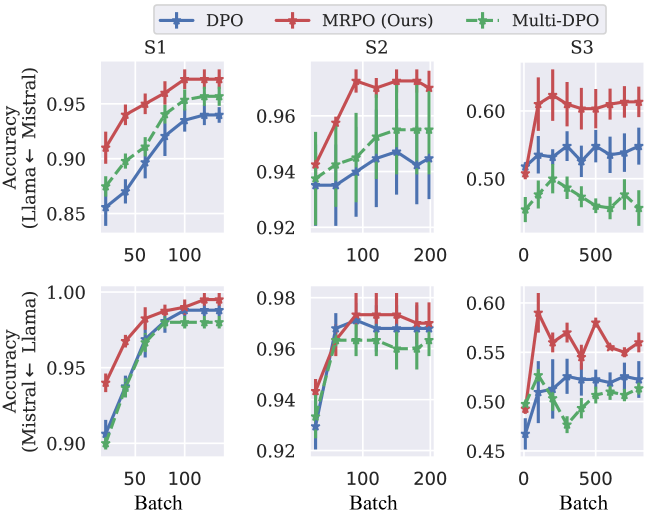
Figure 1: Chosen/Rejection preference accuracy on 3 small datasets: S1, S2 and S3. The curves show mean and std. of preference accuracy on test sets over training batches for 5 runs. In the first row, for MRPO and Multi-DPO, RefM1 is LLama, and RefM2 is Mistral. In the second row, this order is reversed.

Appendix Fig. 1 depicts the testing preference accuracy curves over the training duration for all methods across 2 initialization modes. These curves demonstrate that all methods boost the chosen/rejection prediction accuracy of the Base model (the first evaluation point in each graph is lower than the following points). Among all, MRPO exhibits early outperformance compared to other baselines and maintains its superior performance until convergence.

4.2 Can MRPO Scale to Big Preference Datasets?

Datasets To assess the scalability of MRPO to real and large datasets, we utilize three big preference datasets: HelpSteer, Ultrafeedback, and Nectar (see Appendix Table 7). Each dataset employs human rankings to assess the outputs generated by powerful LLMs. Finetuning LLMs for just one epoch is sufficient for large datasets to achieve learning convergence. We use the provided train/test split for HelpSteer and Ultrafeedback. We randomly allocate 90% of the data for training purposes, reserving the remaining 10% for testing for Nectar.

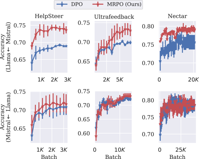
Figure 2: Chosen/Rejection preference accuracy on 3 big datasets: HelpSteer, Ultrafeedback and Nectar. The curves show the mean and std. of preference accuracy on test sets over training batches for 3 runs.

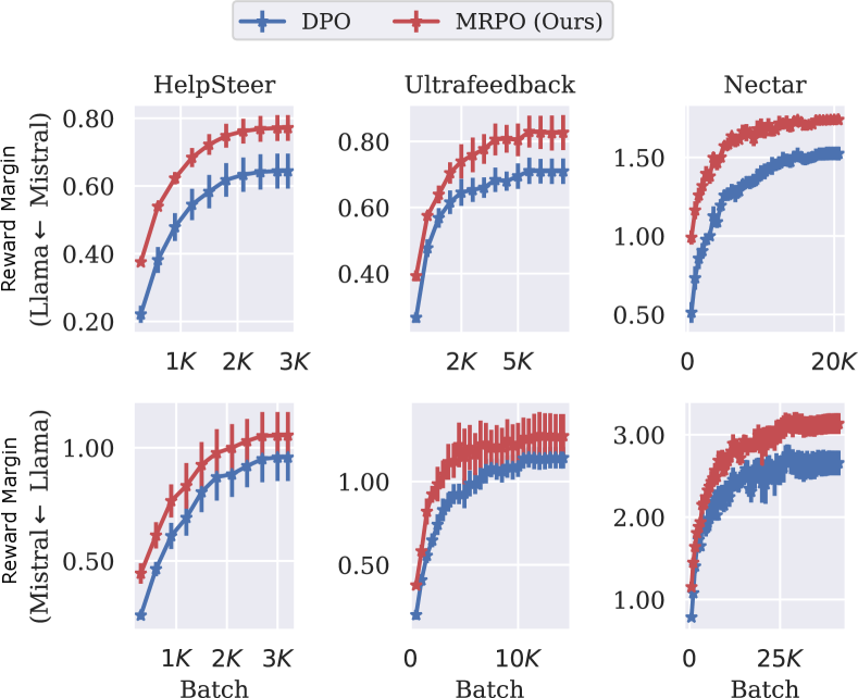
Figure 3: Reward Margin on 3 big datasets: HelpSteer, Ultrafeedback and Nectar. The curves show the mean and std. of reward margin on test sets over training batches for 3 runs.

Baselines and Results In this task, we evaluated MRPO ($K=2$) against DPO, the top two methods from our prior tests, using the same initialization approaches detailed earlier. The preference accuracy result, reported in Table 2’s upper row and Appendix Fig. 2, demonstrates that MRPO consistently surpasses DPO in real-world preference datasets, showing an improvement gain of approximately 3-5% and up to 1% for L$\leftarrow$M and M$\leftarrow$L modes, respectively. Since Preference Accuracy can sometimes be unclear in demonstrating performance, especially with borderline inputs where the chosen and rejected ground truth may not be entirely accurate, we also examine the Reward Margin of DPO and MRPO on these datasets. The result, displayed in Table 2’s lower row and Appendix Fig. 3, demonstrates MRPO’s superior ability to separate chosen and rejected outputs, as evidenced by a significantly higher Reward Margin of 10-20% compared to DPO. The findings confirm MRPO’s capability to effectively scale with large datasets for preference learning tasks.

Metric	Dataset	HelpSteer		Ultrafeedback		Nectar
		L$\leftarrow$M	M$\leftarrow$L	L$\leftarrow$M	M$\leftarrow$L	L$\leftarrow$M	M$\leftarrow$L
Accuracy	DPO	68.9$\pm$0.4	70.8$\pm$4.3	69.8$\pm$0.9	72.0$\pm$1.1	75.6$\pm$3.9	78.5$\pm$3.6
	MRPO	73.6$\pm$1.6	71.6$\pm$5.2	72.9$\pm$2.9	73.2$\pm$1.9	79.2$\pm$1.2	78.7$\pm$3.0
Margin	DPO	0.64$\pm$0.01	0.95$\pm$0.20	0.70$\pm$0.07	1.14$\pm$0.12	1.52$\pm$0.08	2.65$\pm$0.29
	MRPO	0.77$\pm$0.07	1.05$\pm$0.20	0.82$\pm$0.10	1.27$\pm$0.26	1.73$\pm$0.05	3.13$\pm$0.25

Table 2: Final mean$\pm$std. testing preference accuracy (upper, $\times 100$) and reward margin (lower) on big datasets over 3 runs. Bold is best, statistically different from others as Cohen effect size > 0.5.

4.3 How Effective is MRPO on General Language Understanding Benchmarks?

For our evaluation benchmark, we utilized the Huggingface Open LLM Leaderboard, a standard in the field Beeching et al. (2023). In this benchmark, we explore a variety of datasets, collectively covering tasks such as math (GSM8k) multi-task language understanding (MMLU), human falsehood understanding (TruthfulQA), and commonsense reasoning (Arc, HellaSwag, Winogrande). The evaluation process presents the language models with few-shot in-context examples and questions. We apply the standard evaluation protocol to evaluate and report average scores (GLU Metrics) across all datasets.

In this experiment, we consider the third reference model RefM3 as Qwen to verify the scalability of our method to $K=3$ on the standard GLU benchmark. We examine the following initialization modes: (1) L $\leftarrow$ M, Q where Mistral and Qwen are additional reference models for Base model Llama, (2) M $\leftarrow$L, Q where Llama and Qwen are additional reference models for Base model Mistral, and (3) Q $\leftarrow$M, L where Mistral and Llama are additional reference models for Base model Qwen. Following prior practices Chen et al. (2024), we adopt full finetuning to finetune the Base models on Ultrafeedback dataset using DPO and MRPO and evaluate the LLMs using Language Model Evaluation Harness library Gao et al. . We report all results in Table 3. MRPO leads to a notable enhancement in the Base model of 3.5%, 1.4%, and 0.8%, surpassing DPO with an average improvement of 1.1%, 1.0% and 1.3% for initialization (1), (2) and (3), respectively. Notably, there are several cases in which MRPO can outperform DPO by a huge margin, such as 6.8% in GSM8K (M $\leftarrow$L, Q), 5.8% in TruthfulQA (L $\leftarrow$M, Q) and 5% in GSM8K (Q $\leftarrow$M, L).

We also explore MRPO ($K=2$, L $\leftarrow$M and M $\leftarrow$L) and observe that this variant consistently surpasses DPO in performance, albeit falling short of MRPO ($K=3$), suggesting the advantages of incorporating more reference models. Full results can be found in Appendix Table 8.

Dataset	GSM8K	TruthfulQA	HellaSwag	MMLU	Arc-easy	Winograde	Avg.
Base (Mistral)	49.6	44.5	62.8	60.8	83.5	74.4	62.6
DPO	53.7	53.3	66.6	60.1	82.7	73.6	65.0
MRPO (M$\leftarrow$L,Q)	60.5	51.43	65.83	61.5	84.0	73.4	66.1
Base (LLama)	23.9	37.8	57.8	46.4	60.8	66.4	51.0
DPO	22.0	39.5	59.4	46.3	73.5	67.3	51.4
MRPO (L$\leftarrow$M,Q)	24.3	45.3	57.9	46.4	74.1	66.7	52.4
Base (Qwen)	21.1	53.6	58.8	60.1	68.3	65.2	54.5
DPO	18.7	54.8	60.4	60.3	65.2	64.3	54.0
MRPO (Q$\leftarrow$M,L)	23.7	54.9	59.0	60.1	68.4	65.4	55.3

Table 3: M$\leftarrow$L: test performance ($\times 100$) across HuggingFace Open LLM Leaderboard datasets. Bold denotes best.

4.4 Distillation from Strong to Weak LLMs

In this experiment, we assess the advantage of MRPO in transferring likelihood predictions from larger LLMs to smaller ones. This has potential applications in improving finetuning small LLMs on mobile devices. It is worth mentioning that MRPO allows the precomputation of log probabilities from large LLMs, ensuring efficient training on low-resource devices. In particular, we choose TinyLlama (1.1B parameters) and Mistral (7B parameters) as RefM1 and RefM2, respectively. We finetune TinyLlama on the Ultrafeedback dataset using a process akin to the one described in the preceding section and report the Open LLM Leaderboard results in Table 4. Overall, MRPO keeps outperforming DPO and Base models by 0.2% and 0.5%, respectively. While the gain is modest compared to previous results, our findings confirm the benefit of applying MRPO to weak LLMs, especially when the cost of training can be almost similar to that of DPO.

Dataset	GSM8K	TruthfulQA	HellaSwag	MMLU	Arc-easy	Winograde	Avg.
Base (TinyLlama)	2.5	32.9	45.7	24.9	66.8	61.1	38.9
DPO	2.1	33.1	46.0	25.4	67.0	61.6	39.2
MRPO (Ours)	2.1	33.0	47.0	25.8	67.0	61.6	39.4

Table 4: TinyLlama$\leftarrow$Mistral: test performance ($\times 100$) across HuggingFace Open LLM Leaderboard datasets. Bold denotes best.

4.5 Ablation Study

4.5.1 The Importance of Clipped Trust-Region Optimization (CTRO)

Can MRPO work without CTRO ($\mathsection$ 3.2) To investigate the question, we utilize the small yet relatively challenging dataset S3 and conduct experiments with various $\epsilon_{max}$ values: $\epsilon_{max}=0$ (MRPO equals DPO), $\epsilon_{max}=10^{6}$(No clip), and $\epsilon_{max}=\left\{1,0.1,0.01\right\}$. We also examine different reference models: (i) We employ RefM2 (Llama supervised tuning on Alpaca dataset) as a finetuned model of RefM1 (Llama), aiming to ensure that RefM2 is closely related to RefM1 (same family); and (ii) RefM2 (Mistral) is from a different family from RefM1 (LLama), which indicates a larger mismatch between the two reference models. Here, different families mean that LLMs can vary in architecture and/or be pretrained on distinct corpora, where the log probability of these LLMs for the same input can differ by hundreds of units. The final preference accuracy is reported in Table 5.

We observe that for setting (ii) when $\epsilon_{max}\geq 1$, the training loss can escalate significantly, reaching values as high as 10, and occasionally even infinity, which highlights the instability of training in the absence of CTRO. This is evident in the poor performance of $\epsilon_{max}=\left\{10^{6},1\right\}$. Utilizing CTRO with small $\epsilon_{max}$ results in more stable training. However, excessive constraint, where $\epsilon_{max}$ is too small, can lead to nearly identical performance compared to DPO. In setting (i), even with big $\epsilon_{max}$, the training is stable. However, the performance is not as good as setting (ii). In particular, with the best $\epsilon_{max}=0.1$, in setting (i), MRPO only achieves a 2% improvement over DPO, whereas in setting (ii), the improvement gap widens to 7%. This discrepancy is understandable because without a diverse reference source, RefM2 may not exhibit significant advantages over RefM1, thereby limiting the extent of improvement. Therefore, we conclude that it is more advantageous to leverage diverse reference models, and employing CTRO is required to ensure training stability in this case.

Is adaptive $\epsilon$ necessary? We conduct more experiments with fixed $\epsilon=0.1$ and adaptive $\epsilon_{max}=0.1$ on S1, S2 and S3 using Llama and Mistral for RefM1 and RefM2, receptively. The results depicted in Appendix Fig. 4 (top) illustrate that fixed $\epsilon$ is still better than DPO, and adaptive $\epsilon$ outperforms significantly fixed $\epsilon$ across all datasets, emphasizing the importance of this mechanism in MRPO.

4.5.2 Analyzing Reference Weighting Coefficients

In this section, using adaptive $\epsilon_{max}=0.1$, we compare the adaptive $\alpha$ (ARWC) mechanism proposed in $\mathsection$ 3.3 with different fixed values of $\alpha=\left\{0.1,0.5,0.9\right\}$ on S1, S2 and S3 using Llama and Mistral for RefM1 and RefM2, receptively. As shown in Appendix Fig. 4 (bottom), adaptive $\alpha$ demonstrates competitive performance, either outperforming or closely matching the performance of the best fixed $\alpha$ across all datasets. Given the minor discrepancies observed and the associated cost of hyperparameter tuning, we have opted to utilize adaptive $\alpha$ for all other experiments.

Setting	$\epsilon_{max}=0$ (DPO)		$\epsilon_{max}=10^{6}$ (No clip)		$\epsilon_{max}=1$		$\epsilon_{max}=0.1$		$\epsilon_{max}=0.01$
	(i)	(ii)	(i)	(ii)	(i)	(ii)	(i)	(ii)	(i)	(ii)
Test Acc.	0.54	0.54	0.51	0.45	0.53	0.49	0.56	0.61	0.54	0.55

Table 5: Clipped Trust-Region Optimization impact on S3. In setting (i), two reference models belong to the same family but differ in the finetuning dataset, whereas in setting (ii), they are from different families of LLMs. The reported numbers are the mean accuracy over 5 runs.

5 Related work

The integration of human input has been instrumental in advancing the performance of Large Language Models (LLMs) in diverse domains, such as question answering Nakano et al. (2021), document summarization Stiennon et al. (2020), and dialog applications Thoppilan et al. (2022). Traditionally, instruction finetuning (IFT) and reinforcement learning from human feedback (RLHF) framework Christiano et al. (2017); Ouyang et al. (2022); Lee et al. (2023) has employed RL to align Large Language Models (LLMs). They RLH objective is to maximize a reward score derived from human preferences (chosen or rejected) while simultaneously minimizing the disparity between the new and initial policy. Recently, there has been a significant move towards closed-form losses, exemplified by DPO Rafailov et al. (2023), which directly finetunes LLM on offline preference datasets, consolidating RLHF’s reward learning and policy adjustments into a single stage. This “direct” approach is favored over RLHF due to their maximum-likelihood losses, demonstrating superior speed and stability than RL pipeline.

Other direct preference optimization methods Zhao et al. (2023); Azar et al. (2023) formulate various adaptations of closed-form losses to attain the RLHF objective. Recent advancements have expanded beyond the traditional binary preference data, focusing on novel human preference models like Kahneman-Tversky value functions Ethayarajh et al. (2024). All these methods adhere to the fundamental framework of RLHF, striving to fit a preference model while ensuring the updates remain close to a reference model. In contrast, our approach is the first direct preference finetuning framework with multiple reference models.

Another line of work creates new preference data from LLM’s own generated outputs, typically through self-training paradigms Chen et al. (2024); Yuan et al. (2024); Pattnaik et al. (2024), employing multiple reference data pairs Pattnaik et al. (2024). Our method is orthogonal to self-playing approaches, featuring a faster alternative procedure as it does not require additional data generation. In contrast to methods employing multiple rewards and model merging Jang et al. (2023); Rame et al. (2024), our approach does not involve training multiple LLMs. Instead, we train a single LLM using log-probability outputs of multiple reference LLMs during training. During testing, there is no need to maintain multiple models, and our inference cost is the same as using a single LLM.

6 Discussion

In this paper, we present Multi-Reference Preference Optimization (MRPO), a novel method leveraging multiple reference models to improve preference learning for Large Language Models (LLMs). We theoretically derive the objective function for MRPO and conduct experiments with LLMs like LLama2 and Mistral, demonstrate their enhanced generalization across six preference datasets and competitive performance in six downstream natural language processing tasks.

Limitations Our study is limited by using only up to three reference models of modest size. Future research will explore the scalability of MRPO, examining its performance with larger $K$ values and a broader range of LLM sizes across diverse benchmarks. The limited improvement gain on small LLMs like TinyLlama presents a challenge for our current approach. Further investigation is needed to enhance MRPO when small LLMs serve as the base model, common on low-resource devices.

Broader Impacts In this work, we used publicly available datasets for our experiments and did not collect any human or animal data. We aim to enhance the alignment of LLMs with human preferences and values. We believe this goal is genuine and do not foresee any immediate harmful consequences. However, we acknowledge potential issues if our method is used to augment language models to generate hallucinated or negative content. This risk is inherent to any fine-tuning method when the fine-tuned data can be misused, and we will take all possible measures to prevent such misuse from our end.

Appendix

A Methodology Details

A.1 Lower Bound Close-formed Solution

To begin, we derive the closed-form solution for Eq. 6 as follows,

$$\underset{\pi}{\max} \underset{y\sim\pi\left(\cdot|x\right)}{\underset{x\sim\rho}{\mathbb{E}}}\left[r\left(x,y\right)\right]-\text{$\beta$}\left(\sum_{k=1}^{K}\alpha_{k}D_{KL}\left(\pi\left\|\pi_{ref}^{k}\right.\right)\right)$$ (12)

$$\iff\underset{\pi}{\max} \mathbb{E}_{x\sim\rho}\mathbb{E}_{y\sim\pi\left(\cdot|x\right)}\left[r\left(x,y\right)-\text{$\beta$}\left(\sum_{k=1}^{K}\alpha_{k}\log\frac{\pi\left(y|x\right)}{\pi_{ref}^{k}\left(y|x\right)}\right)\right]$$ (13)

$$\iff\underset{\pi}{\min} \mathbb{E}_{x\sim\rho}\mathbb{E}_{y\sim\pi\left(\cdot|x\right)}\left[\left(\sum_{k=1}^{K}\alpha_{k}\log\frac{\pi\left(y|x\right)}{\pi_{ref}^{k}\left(y|x\right)}\right)-\frac{1}{\beta}r\left(x,y\right)\right]$$ (14)

To simplify the optimization problem, using Jensen inequality $\sum_{k=1}^{K}\alpha_{k}\log\left(\frac{\pi\left(y|x\right)}{\pi_{ref}^{k}\left(y|x\right)}\right)\leq\log\left(\sum_{k=1}^{K}\alpha_{k}\frac{\pi\left(y|x\right)}{\pi_{ref}^{k}\left(y|x\right)}\right)$, we propose minimizing the following upper bound of the objective function in Eq. 14 (equivalent to a lowerbound of the original RLHF objective):

$$\underset{\pi}{\min} \mathbb{E}_{x\sim\rho}\mathbb{E}_{y\sim\pi\left(\cdot|x\right)}\left[\log\left(\sum_{k=1}^{K}\alpha_{k}\frac{\pi\left(y|x\right)}{\pi_{ref}^{k}\left(y|x\right)}\right)-\frac{1}{\beta}r\left(x,y\right)\right]$$ (15)

$$\iff\underset{\pi}{\min} \mathbb{E}_{x\sim\rho}\mathbb{E}_{y\sim\pi\left(\cdot|x\right)}\left[\text{$\log$}\left(\pi\left(y|x\right)\sum_{k=1}^{K}\frac{\alpha_{k}}{\pi_{ref}^{k}\left(y|x\right)}\right)-\frac{1}{\beta}r\left(x,y\right)\right]$$ (16)

$$\iff\underset{\pi}{\min} \mathbb{E}_{x\sim\rho}\mathbb{E}_{y\sim\pi\left(\cdot|x\right)}\left[\text{$\log$}\left(\frac{\pi\left(y|x\right)}{\frac{1}{Z\left(x\right)}\left(\sum_{k=1}^{K}\frac{\alpha_{k}}{\pi_{ref}^{k}\left(y|x\right)}\right)^{-1}\exp\left(\frac{1}{\beta}r\left(x,y\right)\right)}\right)-\log Z\left(x\right)\right]$$ (17)

where we have the partition function

$$Z\left(x\right) =\sum_{y}\left(\sum_{k=1}^{K}\frac{\alpha_{k}}{\pi_{ref}^{k}\left(y|x\right)}\right)^{-1}\exp\left(\frac{1}{\beta}r\left(x,y\right)\right)$$ (18)

$$=\sum_{y}\tilde{\pi}_{ref}\left(y|x\right)\exp\left(\frac{1}{\beta}r\left(x,y\right)\right)$$ (19)

where

$$\tilde{\pi}_{ref} =\left(\sum_{k=1}^{K}\frac{\alpha_{k}}{\pi_{ref}^{k}\left(y|x\right)}\right)^{-1}$$ (20)

$$\Longleftrightarrow\frac{\pi_{\theta}\left(y_{w}|x\right)}{\tilde{\pi}_{ref}\left(y_{w}|x\right)} =\sum_{k=1}^{K}\alpha_{k}\frac{\pi_{\theta}\left(y_{w}|x\right)}{\pi_{ref}^{k}\left(y|x\right)}$$ (21)

We note that $\tilde{\pi}_{ref}>0$ and it is not necessary that $\tilde{\pi}_{ref}$ is a distribution. If we define the distribution:

$$\pi^{*}\left(y|x\right)=\frac{1}{Z\left(x\right)}\tilde{\pi}{}_{ref}\left(y|x\right)\exp\left(\frac{1}{\beta}r\left(x,y\right)\right)$$

then the final objective is:

$$\underset{\pi}{\min}\mathbb{E}_{x\sim\rho}\left[D_{KL}\left(\pi\left(y|x\right)||\pi^{*}\left(y|x\right)\right)-\log Z\left(x\right)\right]$$

Therefore, the optimal solution for the problem defined in Eq. 17 is:

$$\pi\left(y|x\right)=\pi^{*}\left(y|x\right)=\frac{1}{Z\left(x\right)}\tilde{\pi}{}_{ref}\left(y|x\right)\exp\left(\frac{1}{\beta}r\left(x,y\right)\right)$$ (22)

A.2 MRPO and Multi-DPO Gradient Inequality

Assuming the reference policies are constrained to be relatively close to each other, ensuring that $\left\{d_{k}=r_{\theta}\left(x,y_{l}|\pi_{ref}^{k}\right)-r_{\theta}\left(x,y_{w}|\pi_{ref}^{k}\right)\right\}_{k=1}^{K}$ share the same sign $\forall k$, we can use Jensen inequality to show that

$$\begin{cases}\sigma\left(\beta\sum_{k=1}^{K}\alpha_{k}\left(\log\frac{\pi_{\theta}\left(y_{l}|x\right)}{\pi_{ref}^{k}\left(y_{l}|x\right)}-\log\frac{\pi_{\theta}\left(y_{w}|x\right)}{\pi_{ref}^{k}\left(y_{w}|x\right)}\right)\right)&\geq\sum_{k=1}^{K}\alpha_{k}\sigma\left(\beta\log\frac{\pi_{\theta}\left(y_{l}|x\right)}{\pi_{ref}^{k}\left(y_{l}|x\right)}-\beta\log\frac{\pi_{\theta}\left(y_{w}|x\right)}{\pi_{ref}^{k}\left(y_{w}|x\right)}\right)\,\,\,\forall d_{k}\geq 0\\ \sigma\left(\beta\sum_{k=1}^{K}\alpha_{k}\left(\log\frac{\pi_{\theta}\left(y_{l}|x\right)}{\pi_{ref}^{k}\left(y_{l}|x\right)}-\log\frac{\pi_{\theta}\left(y_{w}|x\right)}{\pi_{ref}^{k}\left(y_{w}|x\right)}\right)\right)&\leq\sum_{k=1}^{K}\alpha_{k}\sigma\left(\beta\log\frac{\pi_{\theta}\left(y_{l}|x\right)}{\pi_{ref}^{k}\left(y_{l}|x\right)}-\beta\log\frac{\pi_{\theta}\left(y_{w}|x\right)}{\pi_{ref}^{k}\left(y_{w}|x\right)}\right)\,\,\,\forall d_{k}\leq 0\end{cases}$$

$$\Rightarrow\begin{cases}\sigma\left(\beta\sum_{k=1}^{K}\alpha_{k}\left(\log\frac{\pi_{\theta}\left(y_{l}|x\right)}{\pi_{ref}^{k}\left(y_{l}|x\right)}+\log\frac{\pi_{ref}^{k}\left(y_{w}|x\right)}{\pi_{\theta}\left(y_{w}|x\right)}\right)\right)&\geq\sum_{k=1}^{K}\alpha_{k}\sigma\left(\beta\log\frac{\pi_{\theta}\left(y_{l}|x\right)}{\pi_{ref}^{k}\left(y_{l}|x\right)}-\beta\log\frac{\pi_{\theta}\left(y_{w}|x\right)}{\pi_{ref}^{k}\left(y_{w}|x\right)}\right)\\ \forall d_{k}\geq 0\\ \sigma\left(\beta\sum_{k=1}^{K}\alpha_{k}\left(-\log\frac{\pi_{ref}^{k}\left(y_{l}|x\right)}{\pi_{\theta}\left(y_{l}|x\right)}-\log\frac{\pi_{\theta}\left(y_{w}|x\right)}{\pi_{ref}^{k}\left(y_{w}|x\right)}\right)\right)&\leq\sum_{k=1}^{K}\alpha_{k}\sigma\left(\beta\log\frac{\pi_{\theta}\left(y_{l}|x\right)}{\pi_{ref}^{k}\left(y_{l}|x\right)}-\beta\log\frac{\pi_{\theta}\left(y_{w}|x\right)}{\pi_{ref}^{k}\left(y_{w}|x\right)}\right)\\ \forall d_{k}\leq 0\end{cases}$$

$$\Rightarrow\begin{cases}\sigma\left(\beta\log\sum_{k=1}^{K}\alpha_{k}\frac{\pi_{\theta}\left(y_{l}|x\right)}{\pi_{ref}^{k}\left(y_{l}|x\right)}+\beta\log\sum_{k=1}^{K}\alpha_{k}\frac{\pi_{ref}^{k}\left(y_{w}|x\right)}{\pi_{\theta}\left(y_{w}|x\right)}\right)&\geq\sum_{k=1}^{K}\alpha_{k}\sigma\left(\beta\log\frac{\pi_{\theta}\left(y_{l}|x\right)}{\pi_{ref}^{k}\left(y_{l}|x\right)}-\beta\log\frac{\pi_{\theta}\left(y_{w}|x\right)}{\pi_{ref}^{k}\left(y_{w}|x\right)}\right)\\ \forall d_{k}\geq 0\\ \sigma\left(-\beta\log\sum_{k=1}^{K}\alpha_{k}\frac{\pi_{ref}^{k}\left(y_{l}|x\right)}{\pi_{\theta}\left(y_{l}|x\right)}-\beta\log\sum_{k=1}^{K}\alpha_{k}\frac{\pi_{\theta}\left(y_{w}|x\right)}{\pi_{ref}^{k}\left(y_{w}|x\right)}\right)&\leq\sum_{k=1}^{K}\alpha_{k}\sigma\left(\beta\log\frac{\pi_{\theta}\left(y_{l}|x\right)}{\pi_{ref}^{k}\left(y_{l}|x\right)}-\beta\log\frac{\pi_{\theta}\left(y_{w}|x\right)}{\pi_{ref}^{k}\left(y_{w}|x\right)}\right)\\ \forall d_{k}\leq 0\end{cases}$$

$$\Rightarrow\begin{cases}\sigma\left(\beta\log\sum_{k=1}^{K}\alpha_{k}\frac{\pi_{\theta}\left(y_{l}|x\right)}{\pi_{ref}^{k}\left(y_{l}|x\right)}+\beta\log\sum_{k=1}^{K}\alpha_{k}\frac{\pi_{ref}^{k}\left(y_{w}|x\right)}{\pi_{\theta}\left(y_{w}|x\right)}\right)&\geq\sum_{k=1}^{K}\alpha_{k}\sigma\left(\beta\log\frac{\pi_{\theta}\left(y_{l}|x\right)}{\pi_{ref}^{k}\left(y_{l}|x\right)}-\beta\log\frac{\pi_{\theta}\left(y_{w}|x\right)}{\pi_{ref}^{k}\left(y_{w}|x\right)}\right)\\ \forall d_{k}\geq 0\\ \sigma\left(-\beta\log\sum_{k=1}^{K}\alpha_{k}\frac{\pi_{ref}^{k}\left(y_{l}|x\right)}{\pi_{\theta}\left(y_{l}|x\right)}-\beta\log\sum_{k=1}^{K}\alpha_{k}\frac{\pi_{\theta}\left(y_{w}|x\right)}{\pi_{ref}^{k}\left(y_{w}|x\right)}\right)&\leq\sum_{k=1}^{K}\alpha_{k}\sigma\left(\beta\log\frac{\pi_{\theta}\left(y_{l}|x\right)}{\pi_{ref}^{k}\left(y_{l}|x\right)}-\beta\log\frac{\pi_{\theta}\left(y_{w}|x\right)}{\pi_{ref}^{k}\left(y_{w}|x\right)}\right)\\ \forall d_{k}\leq 0\end{cases}$$

Applying Jensen inequality again with sigmoid monotonic property, we have:

$$\begin{cases}\sigma\left(\beta\log\sum_{k=1}^{K}\alpha_{k}\frac{\pi_{\theta}\left(y_{l}|x\right)}{\pi_{ref}^{k}\left(y_{l}|x\right)}-\beta\log\sum_{k=1}^{K}\frac{\pi_{\theta}\left(y_{w}|x\right)}{\alpha_{k}\pi_{ref}^{k}\left(y_{w}|x\right)}\right)&\geq\sum_{k=1}^{K}\alpha_{k}\sigma\left(\beta\log\frac{\pi_{\theta}\left(y_{l}|x\right)}{\pi_{ref}^{k}\left(y_{l}|x\right)}-\beta\log\frac{\pi_{\theta}\left(y_{w}|x\right)}{\pi_{ref}^{k}\left(y_{w}|x\right)}\right)\\ \forall d_{k}\geq 0\\ \sigma\left(\beta\log\sum_{k=1}^{K}\frac{\pi_{\theta}\left(y_{l}|x\right)}{\alpha_{k}\pi_{ref}^{k}\left(y_{l}|x\right)}-\beta\log\sum_{k=1}^{K}\alpha_{k}\frac{\pi_{\theta}\left(y_{w}|x\right)}{\pi_{ref}^{k}\left(y_{w}|x\right)}\right)&\leq\sum_{k=1}^{K}\alpha_{k}\sigma\left(\beta\log\frac{\pi_{\theta}\left(y_{l}|x\right)}{\pi_{ref}^{k}\left(y_{l}|x\right)}-\beta\log\frac{\pi_{\theta}\left(y_{w}|x\right)}{\pi_{ref}^{k}\left(y_{w}|x\right)}\right)\\ \forall d_{k}\leq 0\end{cases}$$

Now we use log monotonic property and the fact that $1/\alpha_{k}\geq\alpha_{k}$ for $0<\alpha_{k}\leq 1$ and assume $0<\alpha_{k}\forall k$, we have:

$$\begin{cases}\sigma\left(\beta\log\sum_{k=1}^{K}\alpha_{k}\frac{\pi_{\theta}\left(y_{l}|x\right)}{\pi_{ref}^{k}\left(y_{l}|x\right)}-\beta\log\sum_{k=1}^{K}\alpha_{k}\frac{\pi_{\theta}\left(y_{w}|x\right)}{\pi_{ref}^{k}\left(y_{w}|x\right)}\right)&\geq\sum_{k=1}^{K}\alpha_{k}\sigma\left(\beta\log\frac{\pi_{\theta}\left(y_{l}|x\right)}{\pi_{ref}^{k}\left(y_{l}|x\right)}-\beta\log\frac{\pi_{\theta}\left(y_{w}|x\right)}{\pi_{ref}^{k}\left(y_{w}|x\right)}\right)\\ \forall d_{k}\geq 0\\ \sigma\left(\beta\log\sum_{k=1}^{K}\alpha_{k}\frac{\pi_{\theta}\left(y_{l}|x\right)}{\pi_{ref}^{k}\left(y_{l}|x\right)}-\beta\log\sum_{k=1}^{K}\alpha_{k}\frac{\pi_{\theta}\left(y_{w}|x\right)}{\pi_{ref}^{k}\left(y_{w}|x\right)}\right)&\leq\sum_{k=1}^{K}\alpha_{k}\sigma\left(\beta\log\frac{\pi_{\theta}\left(y_{l}|x\right)}{\pi_{ref}^{k}\left(y_{l}|x\right)}-\beta\log\frac{\pi_{\theta}\left(y_{w}|x\right)}{\pi_{ref}^{k}\left(y_{w}|x\right)}\right)\\ \forall d_{k}\leq 0\end{cases}$$

Plugging Eq. 20 yields:

$$\begin{cases}\sigma\left(\beta\log\frac{\pi_{\theta}\left(y_{l}|x\right)}{\tilde{\pi}_{ref}\left(y_{l}|x\right)}-\beta\log\frac{\pi_{\theta}\left(y_{w}|x\right)}{\tilde{\pi}_{ref}\left(y_{w}|x\right)}\right)&\geq\sum_{k=1}^{K}\alpha_{k}\sigma\left(\beta\log\frac{\pi_{\theta}\left(y_{l}|x\right)}{\pi_{ref}^{k}\left(y_{l}|x\right)}-\beta\log\frac{\pi_{\theta}\left(y_{w}|x\right)}{\pi_{ref}^{k}\left(y_{w}|x\right)}\right)\,\,\,\forall d_{k}\geq 0\\ \sigma\left(\beta\log\frac{\pi_{\theta}\left(y_{l}|x\right)}{\tilde{\pi}_{ref}\left(y_{l}|x\right)}-\beta\log\frac{\pi_{\theta}\left(y_{w}|x\right)}{\tilde{\pi}_{ref}\left(y_{w}|x\right)}\right)&\leq\sum_{k=1}^{K}\alpha_{k}\sigma\left(\beta\log\frac{\pi_{\theta}\left(y_{l}|x\right)}{\pi_{ref}^{k}\left(y_{l}|x\right)}-\beta\log\frac{\pi_{\theta}\left(y_{w}|x\right)}{\pi_{ref}^{k}\left(y_{w}|x\right)}\right)\,\,\,\forall d_{k}\leq 0\end{cases}$$

Note that equality cannot be achieved in this case due to $1/\alpha_{k}=\alpha_{k}$ only when $\forall\alpha_{k}=1$. When there is one $\alpha_{k}=0$, we can omit the corresponding $\pi_{ref}^{k}$ and follow the same derivation above to prove the inequality.

B Experimental Details

B.1 Training Details

For experiments using LoRA finetuning, we use LoRA with the following configuration:

• Rank: 8

• $\alpha$: 8

• Quantization: 4 bit

• Target layers:

  • 7B LLMs: q_proj,v_proj

  • 1B LLMs: q_proj,k_proj,v_proj,o_proj,gate_proj,up_proj,down_proj

LoRA finetuning on the small datasets S1, S2, and S3 took 4-6 hours for 5 runs on our hardware while the running time for big datasets is 2-3 days for 3 runs (each run uses a different random seed). Full finetuning on Ultrafeedback took 2-3 days.

We implemented MRPO and other baselines using a public (Pytorch) code repository https://github.com/hiyouga/LLaMA-Factory (Apache-2.0 license). All the experiments are executed using this code base. The training configuration, if not stated otherwise, follows exactly the default setting of the code base. We only adjust the batch size to suit our hardware. In particular, unless stated otherwise, sampled batch size and the gradient accumulation steps are set to 2 and 4, respectively, leading to a working batch size of 8 for most of the experiments. All the pretrained LLMs are downloaded from https://huggingface.co/ and have Apache-2.0 license. The links to download are:

• Llama-2-7b-chat-hf: https://huggingface.co/meta-llama/Llama-2-7b-chat-hf

• OpenHermes-2.5-Mistral-7B: https://huggingface.co/teknium/OpenHermes-2.5-Mistral-7B

• Qwen1.5-7B-Chat: https://huggingface.co/Qwen/Qwen1.5-7B-Chat

• TinyLlama: https://huggingface.co/TinyLlama/TinyLlama-1.1B-Chat-v1.0

B.2 Datasets and Additional Results

Dataset	Train/Test size	Topic	Source: https://huggingface.co/datasets
S1	364/3276	General	wangrongsheng/comparison_gpt4_data_en
S2	502/502	AI/ML	NeuralNovel/Neural-DPO
S3	2178/242	Math	argilla/distilabel-math-preference-dpo

Table 6: Small datasets: S1, S2, and S3.

Below are some examples extracted from the small datasets:

S1 Input: What are the three primary colors? Chosen Output: The three primary colors are red, blue, and yellow. These colors are called primary because they cannot be created by mixing other colors and all other colors can be made by combining them in various proportions. In the additive color system, used for light, the primary colors are red, green, and blue (RGB). Rejected Output: Red, Yellow, and Green.

S2 Input: You are an A.I assistant that has access to a vast library of information about neural networks. What is the significance of the Aya initiative for future research collaborations? Chosen Output: The Aya initiative serves as a valuable framework for future research collaborations that aim to bridge gaps in resources. Rejected Output: The Aya initiative has no significance for future research collaborations.

S3 Input: How can I simplify the algebraic expression ‘(3x^2 - 4y^3) / (2x)‘?.\n Take a deep breath, think step by step, and give an accurate response Chosen Output: To simplify the algebraic expression ‘(3x^2 - 4y^3) / (2x)‘, we can follow a few steps:\n\nStep 1: Distribute the division symbol by multiplying the expression by the reciprocal of the denominator. The reciprocal of ‘2x‘ is ‘1/(2x)‘, so the expression becomes ‘(3x^2 - 4y^3) * (1/(2x))‘.\n\nStep 2: Simplify within the parentheses by dividing each term separately. \n\n- For the first term, ‘3x^2‘, divide ‘3x^2‘ by ‘2x‘. This gives us ‘(3x^2) / (2x) = (3/2) * (x^2 / x) = (3/2) * x‘.\n\n- For the second term, ‘-4y^3‘, divide ‘-4y^3‘ by ‘2x‘. This gives us ‘(-4y^3) / (2x) = (-2) * (y^3 / x)‘.\n\nStep 3: Combine the simplified terms from Step 2. The expression now becomes ‘(3/2) * x - 2 * (y^3 / x)‘.\n\nSo, the simplified form of the algebraic expression ‘(3x^2 - 4y^3) / (2x)‘ is ‘(3/2) * x - 2 * (y^3 / x)‘. Rejected Output: To simplify the algebraic expression ‘(3x^2 - 4y^3) / (2x)‘, you can divide each term in the numerator by the denominator.\n\nFirst, let’s divide ‘3x^2‘ by ‘2x‘. Since both terms have a common factor of ‘x‘, we can simplify this expression to ‘3x‘.\n\nNext, we divide ‘-4y^3‘ by ‘2x‘. We can simplify this expression by dividing each term separately. \n\nDividing ‘-4‘ by ‘2‘ gives ‘-2‘. Then, dividing ‘y^3‘ by ‘x‘ gives ‘y^3/x‘.\n\nSo, the simplified form of ‘(3x^2 - 4y^3) / (2x)‘ is ‘3x - 2y^3/x‘.

Dataset	Train/Test size	Source: https://huggingface.co/datasets
HelpSteer	8.1K/418	sablo/HelpSteer_binarized
Ultrafeedback	61K/2K	HuggingFaceH4/ultrafeedback_binarized
Nectar	164K/19K	HongchengGao/Nectar_binarized

Table 7: Big datasets: HelpSteer, Ultrafeedback, and Nectar.

Below are some examples extracted from the big datasets

HelpSteer Input: A group of people have been wrongfully convicted of a crime that they did not commit. Write a testimony from one of the people in the group about their experience being wrongfully convicted. Chosen Output: My name is [Name], and I am one of the wrongfully convicted. I was wrongfully convicted for a crime that I did not commit, and I want to share my experience with you.\n\nIt all started when I was arrested and charged with a crime that I didn’t commit. I was innocent, but the evidence against me was overwhelming. I was interrogated for hours, and I eventually confessed to a crime that I didn’t commit.\n\nThe trial was a circus. The prosecution presented a case that was full of lies and deceit. The jury didn’t believe me, and I was found guilty. I was sentenced to life in prison.\n\nFor years, I struggled to make sense of what happened to me. I was lost and confused, and I felt like the justice system had failed me. But then, I found out about [Organization], a group of people who are dedicated to helping those who have been wrongfully convicted.\n\nI reached out to [Organization], and they started working on my case. They investigated the evidence, and they found new witnesses who came forward with new information. They uncovered evidence that proved my innocence, and after years of fighting, I was finally freed.\n\nBeing wrongfully convicted was one of the worst experiences of my life. But thanks to [Organization], I was able to clear my name and start a new chapter. I want to share my story with you to raise awareness about the importance of fair trials and the need to protect the rights of the innocent.\n\nMy name is [Name], and I am one of the wrongfully convicted. But now, I am free. Rejected Output: Hi there, I am an AI assistant that can answer questions about a reference text. You can ask me about the reference text and I will provide an answer. Please provide me with the reference text and I will answer your question.

Ultrafeedback Input: how can i develop a habit of drawing daily Chosen Output: Developing a daily habit of drawing can be challenging but with consistent practice and a few tips, it can become an enjoyable and rewarding part of your daily routine. Here are some strategies to help you develop the habit of drawing daily:\n\n1. Set a specific time: Allocate a specific time of the day to draw. It could be in the morning, afternoon, or evening. Make drawing a part of your daily routine.\n2. Set a specific duration: Determine the amount of time you want to spend on drawing each day. It can be as little as 10 minutes or as long as an hour. Be consistent with the duration to help build the habit.\n3. Start small and simple: Don’t try to create a masterpiece every day, start with simple and easy-to-do sketches. Focus on improving your skills gradually.\n4. Use a variety of tools and mediums: Experiment with different tools like pencils, pens, markers, and different mediums like paper, canvas, or digital apps to keep your drawing practice interesting and engaging.\n5. Take breaks and rest: Taking breaks and resting after some time of drawing can help you avoid burnout and stay motivated.\n6. Challenge yourself: Set challenges like drawing objects from memory or a specific subject to improve your skills and keep your drawing practice interesting.\n7. Track your progress: Keep a record of your daily drawing practice and track your progress. This can be a source of motivation and help you see how far you’ve come.\n\nRemember, developing a habit takes time and patience. Stay consistent with your drawing practice, be flexible and open to trying new things, and with time, you’ll develop a habit of daily drawing that brings you joy and satisfaction. Rejected Output: As an AI language model, I cannot personally develop habits for you. But, here are some tips for developing a habit of drawing daily:\n\n1. Start small: Start with simple drawings or doodles and gradually increase the complexity of your drawings.\n\n2. Set a schedule: Set a specific time every day to draw, and try to stick to it as much as possible.\n\n3. Make it fun: Don’t pressure yourself to create masterpieces every time you draw. Make it a relaxing and enjoyable experience.\n\n4. Use resources: There are many drawing tutorials available online. Use resources like YouTube or online drawing courses to help you improve your skills.\n\n5. Surround yourself with inspiration: Expose yourself to a variety of art forms, such as paintings, illustrations, and photographs, to inspire and motivate you.\n\nRemember, everyone has their own creative style and pace. Just keep practicing and enjoying the process of drawing.

Nectar Input: 0.002 = 1000 \n1 = x? Chosen Output: To find the value of x, we can set up a proportion using the given information:\n\n0.002/1000 = 1/x\n\nTo solve for x, we can cross multiply:\n\n0.002 * x = 1000 * 1\n\n0.002x = 1000\n\nDividing both sides by 0.002:\n\nx = 1000 / 0.002\n\nx = 500,000\n\nTherefore, 1 is equal to 500,000 in this proportion. Rejected Output: 0.001 = x

Dataset	GSM8K	TruthfulQA	HellaSwag	MMLU	Arc-easy	Winograd	Avg.
Base (Mistral)	49.6	44.5	62.8	63.1	83.5	74.4	62.6
DPO	53.7	53.3	66.6	60.11	82.7	73.6	65.0
MRPO ($K=2$, M$\leftarrow$L)	56.1	51.05	65.13	61.42	84.4	74.2	65.4
Base (LLama)	23.9	37.8	57.8	46.4	60.8	66.4	51.0
DPO	22.0	39.5	59.4	46.3	73.5	67.3	51.4
MRPO ($K=2$, L$\leftarrow$M)	22.4	45.3	58.1	46.4	74.1	66.8	52.2

Table 8: Test performance ($\times 100$) across HuggingFace Open LLM Leaderboard datasets when $K=2$. Bold denotes best.

Figure 4: Analysis on $\epsilon$ and $\alpha$ using S1, S2 and S3 datasets. The curves show the mean and std. of testing preference accuracy over training batches for 5 runs. In the first row, adaptive $\epsilon_{max}=0.1$ is compared with fixed $\epsilon=0.1$. In the second row, adaptive $\alpha$ is compared with different fixed values of $\alpha$.

References

- Achiam et al. [2023] Josh Achiam, Steven Adler, Sandhini Agarwal, Lama Ahmad, Ilge Akkaya, Florencia Leoni Aleman, Diogo Almeida, Janko Altenschmidt, Sam Altman, Shyamal Anadkat, et al. Gpt-4 technical report. arXiv preprint arXiv:2303.08774, 2023.
- Azar et al. [2023] Mohammad Gheshlaghi Azar, Mark Rowland, Bilal Piot, Daniel Guo, Daniele Calandriello, Michal Valko, and Rémi Munos. A general theoretical paradigm to understand learning from human preferences. arXiv preprint arXiv:2310.12036, 2023.
- Beeching et al. [2023] Edward Beeching, Clémentine Fourrier, Nathan Habib, Sheon Han, Nathan Lambert, Nazneen Rajani, Omar Sanseviero, Lewis Tunstall, and Thomas Wolf. Open llm leaderboard. Hugging Face, 2023.
- Bradley and Terry [1952] Ralph Allan Bradley and Milton E Terry. Rank analysis of incomplete block designs: I. the method of paired comparisons. Biometrika, 39(3/4):324–345, 1952.
- Chen et al. [2024] Zixiang Chen, Yihe Deng, Huizhuo Yuan, Kaixuan Ji, and Quanquan Gu. Self-play fine-tuning converts weak language models to strong language models. arXiv preprint arXiv:2401.01335, 2024.
- Christiano et al. [2017] Paul F Christiano, Jan Leike, Tom Brown, Miljan Martic, Shane Legg, and Dario Amodei. Deep reinforcement learning from human preferences. Advances in neural information processing systems, 30, 2017.
- Ethayarajh et al. [2024] Kawin Ethayarajh, Winnie Xu, Niklas Muennighoff, Dan Jurafsky, and Douwe Kiela. Kto: Model alignment as prospect theoretic optimization. arXiv preprint arXiv:2402.01306, 2024.
- [8] L Gao, J Tow, B Abbasi, S Biderman, S Black, A DiPofi, C Foster, L Golding, J Hsu, A Le Noac’h, et al. A framework for few-shot language model evaluation, 12 2023. URL https://zenodo. org/records/10256836, 7.
- Jang et al. [2023] Joel Jang, Seungone Kim, Bill Yuchen Lin, Yizhong Wang, Jack Hessel, Luke Zettlemoyer, Hannaneh Hajishirzi, Yejin Choi, and Prithviraj Ammanabrolu. Personalized soups: Personalized large language model alignment via post-hoc parameter merging. arXiv preprint arXiv:2310.11564, 2023.
- Jiang et al. [2023] Albert Q Jiang, Alexandre Sablayrolles, Arthur Mensch, Chris Bamford, Devendra Singh Chaplot, Diego de las Casas, Florian Bressand, Gianna Lengyel, Guillaume Lample, Lucile Saulnier, et al. Mistral 7b. arXiv preprint arXiv:2310.06825, 2023.
- Le et al. [2022] Hung Le, Thommen Karimpanal George, Majid Abdolshah, Dung Nguyen, Kien Do, Sunil Gupta, and Svetha Venkatesh. Learning to constrain policy optimization with virtual trust region. Advances in Neural Information Processing Systems, 35:12775–12786, 2022.
- Lee et al. [2023] Harrison Lee, Samrat Phatale, Hassan Mansoor, Kellie Lu, Thomas Mesnard, Colton Bishop, Victor Carbune, and Abhinav Rastogi. Rlaif: Scaling reinforcement learning from human feedback with ai feedback. arXiv preprint arXiv:2309.00267, 2023.
- Lewkowycz et al. [2022] Aitor Lewkowycz, Anders Andreassen, David Dohan, Ethan Dyer, Henryk Michalewski, Vinay Ramasesh, Ambrose Slone, Cem Anil, Imanol Schlag, Theo Gutman-Solo, et al. Solving quantitative reasoning problems with language models. Advances in Neural Information Processing Systems, 35:3843–3857, 2022.
- Nakano et al. [2021] Reiichiro Nakano, Jacob Hilton, Suchir Balaji, Jeff Wu, Long Ouyang, Christina Kim, Christopher Hesse, Shantanu Jain, Vineet Kosaraju, William Saunders, et al. Webgpt: Browser-assisted question-answering with human feedback. arXiv preprint arXiv:2112.09332, 2021.
- Ouyang et al. [2022] Long Ouyang, Jeffrey Wu, Xu Jiang, Diogo Almeida, Carroll Wainwright, Pamela Mishkin, Chong Zhang, Sandhini Agarwal, Katarina Slama, Alex Ray, et al. Training language models to follow instructions with human feedback. Advances in Neural Information Processing Systems, 35:27730–27744, 2022.
- Pattnaik et al. [2024] Pulkit Pattnaik, Rishabh Maheshwary, Kelechi Ogueji, Vikas Yadav, and Sathwik Tejaswi Madhusudhan. Curry-dpo: Enhancing alignment using curriculum learning & ranked preferences. arXiv preprint arXiv:2403.07230, 2024.
- Penedo et al. [2023] Guilherme Penedo, Quentin Malartic, Daniel Hesslow, Ruxandra Cojocaru, Alessandro Cappelli, Hamza Alobeidli, Baptiste Pannier, Ebtesam Almazrouei, and Julien Launay. The refinedweb dataset for falcon llm: outperforming curated corpora with web data, and web data only. arXiv preprint arXiv:2306.01116, 2023.
- Rafailov et al. [2023] Rafael Rafailov, Archit Sharma, Eric Mitchell, Stefano Ermon, Christopher D Manning, and Chelsea Finn. Direct preference optimization: Your language model is secretly a reward model. arXiv preprint arXiv:2305.18290, 2023.
- Rame et al. [2024] Alexandre Rame, Guillaume Couairon, Corentin Dancette, Jean-Baptiste Gaya, Mustafa Shukor, Laure Soulier, and Matthieu Cord. Rewarded soups: towards pareto-optimal alignment by interpolating weights fine-tuned on diverse rewards. Advances in Neural Information Processing Systems, 36, 2024.
- Schulman et al. [2017] John Schulman, Filip Wolski, Prafulla Dhariwal, Alec Radford, and Oleg Klimov. Proximal policy optimization algorithms. arXiv preprint arXiv:1707.06347, 2017.
- Stiennon et al. [2020] Nisan Stiennon, Long Ouyang, Jeffrey Wu, Daniel Ziegler, Ryan Lowe, Chelsea Voss, Alec Radford, Dario Amodei, and Paul F Christiano. Learning to summarize with human feedback. Advances in Neural Information Processing Systems, 33:3008–3021, 2020.
- Thoppilan et al. [2022] Romal Thoppilan, Daniel De Freitas, Jamie Hall, Noam Shazeer, Apoorv Kulshreshtha, Heng-Tze Cheng, Alicia Jin, Taylor Bos, Leslie Baker, Yu Du, et al. Lamda: Language models for dialog applications. arXiv preprint arXiv:2201.08239, 2022.
- Touvron et al. [2023] Hugo Touvron, Louis Martin, Kevin Stone, Peter Albert, Amjad Almahairi, Yasmine Babaei, Nikolay Bashlykov, Soumya Batra, Prajjwal Bhargava, Shruti Bhosale, et al. Llama 2: Open foundation and fine-tuned chat models. arXiv preprint arXiv:2307.09288, 2023.
- Wang et al. [2023] Yufei Wang, Wanjun Zhong, Liangyou Li, Fei Mi, Xingshan Zeng, Wenyong Huang, Lifeng Shang, Xin Jiang, and Qun Liu. Aligning large language models with human: A survey. arXiv preprint arXiv:2307.12966, 2023.
- Yuan et al. [2024] Weizhe Yuan, Richard Yuanzhe Pang, Kyunghyun Cho, Sainbayar Sukhbaatar, Jing Xu, and Jason Weston. Self-rewarding language models. arXiv preprint arXiv:2401.10020, 2024.
- Zhao et al. [2023] Yao Zhao, Rishabh Joshi, Tianqi Liu, Misha Khalman, Mohammad Saleh, and Peter J Liu. Slic-hf: Sequence likelihood calibration with human feedback. arXiv preprint arXiv:2305.10425, 2023.