Trivialized Momentum Facilitates Diffusion Generative Modeling on Lie Groups

Abstract

The generative modeling of data on manifold is an important task, for which diffusion models in flat spaces typically need nontrivial adaptations. This article demonstrates how a technique called ‘trivialization’ can transfer the effectiveness of diffusion models in Euclidean spaces to Lie groups. In particular, an auxiliary momentum variable was algorithmically introduced to help transport the position variable between data distribution and a fixed, easy-to-sample distribution. Normally, this would incur further difficulty for manifold data because momentum lives in a space that changes with the position. However, our trivialization technique creates to a new momentum variable that stays in a simple fixed vector space. This design, together with a manifold preserving integrator, simplifies implementation and avoids inaccuracies created by approximations such as projections to tangent space and manifold, which were typically used in prior work, hence facilitating generation with high-fidelity and efficiency. The resulting method achieves state-of-the-art performance on protein and RNA torsion angle generation and sophisticated torus datasets. We also, arguably for the first time, tackle the generation of data on high-dimensional Special Orthogonal and Unitary groups, the latter essential for quantum problems.

1 Introduction

Diffusion-based [e.g., 40, 15, 9] and flow-based [e.g., 23, 24, 1] generative models have significantly impacted the landscape of various fields such as computer vision, largely due to their remarkable ability in modeling data that follow complicated and/or high-dimensional probability distributions. However, in many application domains, data explicitly reside on manifolds. Note this is different from the popular data manifold assumption which is implicit; here the manifold is a priori fixed due to, e.g., physics. Such cases occur, for example, in protein modeling [37, 45], cell development [20], geographical sciences [42], robotics [38], and high-energy physics [44]. The naive application of standard generative models to these cases via embedding data in ambient Euclidean spaces often results in suboptimal performance [8]. This is partly due to the lack of appropriate geometric inductive biases and potential encounters with singularities [4].

Pioneering works suggest generalizing (continuous) neural ODE [6] to manifold [30, 25, 14] with maximum-likelihood training. [36, 3] develop simulation-free algorithm but their objective is unscalable or biased [26]. Recent milestones, such as Riemannian Score-based Model (RSGM) [8] and Riemannian Diffusion Model (RDM) [16], have successfully demonstrated the potential to extend diffusion models onto Riemannian manifolds. RSGM explores the effectiveness and complexity of various variants of score matching loss on a general manifold and their applicable scenarios, and RDM discusses techniques such as variance reduction for the training objective via importance sampling and likelihood estimation. These models learn to reverse the diffusion process on a manifold, either by utilizing the heat equation defined on the manifold or by extending the Stochastic Differential Equation to the manifold. This is achieved through the employment of Riemannian score matching methods, which serve as simulation-based objectives for the optimization of the model. However, due to the inherent geometric complexity of the data, the training and sampling processes of such models necessitate multiple approximations. In particular, they require the projection of vector field (i.e score) to the tangent space which subsequently serves as the training label for the neural network during training phase. Furthermore, to mitigate numerical integration errors during the sampling process, there is a requirement for the projection of samples to the original data manifold. Moreover, among most scenarios, as these models are simulation-based algorithms, an additional approximation is introduced during the collection of training data from the simulation during training. This process also necessitates the projection of data to the manifold, which is analogous to the sampling phase. The combination of all these three approximations can compromise the quality of generation.

Even more recent advancements, such as Riemannian Flow Matching (RFM) [5] and Scaled-RSGM [26], aim to alleviate training complexities and enhance model scalability through the introduction of simulation-free objectives. Scaled-RSGM achieves this by focusing on Riemannian symmetric spaces, while RFM constructs conditional flows using premetrics. However, it is important to note that both of the approaches still require the aforementioned approximations during the training and sampling phases, which may potentially introduce inaccuracies in the generated results. Furthermore, whether RFM is expressive enough for intricate data distribution was discussed in [26].

In this work, we build upon recent progress in momentum-based optimization [41] and sampling [22] on Lie groups to develop a highly scalable and effective generative model for data on these manifolds. Our approach departs from prior momentum-based generative models [11, 7] due to an additional technique called trivialization, which utilizes the additional group structure and enables us to learn score in a fixed flat space, while still encapsulating the curved geometry without any approximation. It results in a novel Trivialized Diffusion Model (TDM), and our contributions are threefold:

1. We introduce TDM that enables manifold data generative modeling through learning trivialized score function in a fixed flat space, which dramatically improves the generative performance.

2. We leverage a nontrivial Operator Splitting Integrator to stay exactly on the manifold in an accurate and efficient way. The reduction of approximations further improves the generation.

3. We outperform baselines by a large margin on protein/RNA torsion angle datasets. We achieve much higher quality generation on a newly-introduced challenging problem called Pacman. We present the first results on generating $\mathsf{U}(n)$ data corresponding to quantum evolutions, and high dim $\mathsf{SO}(n)$ data too; these results are also appealing.

2 Preliminaries

Euclidean Diffusion Model, kinetic Langevin, and Lie group are briefly reviewed in Appendix A.

3 Method

In this section, we will discuss how to perform generative modeling of data distribution on a class of smooth Riemannian manifolds, namely Lie groups, by only learning a score function in a fixed Euclidean space. Our goal is to recover the scenario of Euclidean generative modeling to the maximum by leveraging the group structure of the Lie group apart from its Riemannian manifold structure. To achieve this, we explore a specific manifold extension of Kinetic Langevin dynamics [33], which contains an additional variable known as momentum. Importantly, a direct introduction of the momentum would not simplify the situation, since the momentum lives in a changing tangent space as the position moves. Fortunately, the group structure of the Lie group enables the design of a trivialized momentum that stays in a Lie algebra for the whole time, which is a simple fixed Euclidean space that suits our needs. In the sequel, we will discuss how the technique of trivialization can help completely avoid challenges posed by the curved geometry in an exact, analytical fashion, without resorting to complicated differential geometry notions such as parallel transport, and certainly no need for approximations, projections and retractions.

In the following, we first introduce a forward process that converges to an easy-to-sample distribution with such trivialized momentum. We derive the time reversal of such a process, which can serve as a backward generative process. We discuss methods to efficiently learn the drift of the backward process. Finally, we introduce a numerical integrator that achieves high accuracy and preserves the manifold structure of the Lie group.

3.1 Trivialized Kinetic Langevin Dynamics on Lie Group as Noising Process

Kong and Tao [22] appropriately added noise to variational Lie group optimization dynamics [41] and constructed the following kinetic Langevin sampling dynamics on Lie groups:

$$\begin{cases}\dot{g_{t}}=T_{e}\mathsf{L}_{g_{t}}\xi_{t},\\ {\mathrm{d}}\xi_{t}=-\gamma(t)\xi_{t}{\mathrm{d}}t-T_{g}\mathsf{L}_{g_{t}^{-1}}(\nabla U(g_{t})){\mathrm{d}}t+\sqrt{2\gamma(t)}{\mathrm{d}}W^{\mathfrak{g}}_{t},\end{cases}$$ (1)

where $g_{t},\xi_{t}\in G\times\mathfrak{g},\;\forall t\geq 0$, here $G$ denotes a Lie group and $\mathfrak{g}$ denotes its associated Lie algebra, ${\mathrm{d}}W^{\mathfrak{g}}_{t}$ is the Brownian motion on Lie algebra $\mathfrak{g}$, $\nabla U$ is the riemannian gradient of $U$, and $U:G\rightarrow\mathbb{R}$ is a potential function. $\xi_{t}$ is the left-trivialized momentum at time $t$ and $T_{e}\mathsf{L}_{g_{t}}\xi_{t}$ is the true momentum.

They also proved [22] that for connected compact Lie groups, which will be our setup, (1) converges, under Lipschitzness of $\nabla U$, exponentially fast to its invariant distribution, which is

$$\pi_{*}(g,\xi)=\frac{1}{Z}\exp\Big{(}-U(g)-\frac{1}{2}\langle\xi,\xi\rangle\Big{)}{\mathrm{d}}g{\mathrm{d}}\xi,$$ (2)

where ${\mathrm{d}}g$ denotes the Haar measure, ${\mathrm{d}}\xi$ denotes the Lebesgue measure on $\mathfrak{g}$, and $Z$ is the normalizing constant. Dynamic (1) is a generalization of the Euclidean kinetic Langevin equation on $\mathbb{R}^{k}$ to general Lie groups ($\mathbb{R}^{k}$ is a Lie group with vector addition being the group operation).

By Peter-Weyl Theorem, a connected compact Lie group can be represented as closed subgroups of $\operatorname{GL}(n,\mathbb{C)}$ [21], i.e. the group of $n\times n$ invertible matrices with entries in $\mathbb{C}$. We want to construct a forward noising process based on (1) by choosing a potential $U$ that corresponds to an easy-to-sample distribution on $G$. In the case of connected compact Lie groups, we pick the natural choice, which is the uniform distribution on $G$, to be the invariant distribution (note in this case, the limiting measure is Haar in $g$ which is easy to sample from; see [31]). This means that $U(g)=0$ and the corresponding $\nabla U(g)=0$. In this case, we derive the following dynamic as the forward noising process,

$$\begin{cases}\dot{g_{t}}=g_{t}\xi_{t},\\ {\mathrm{d}}\xi_{t}=-\gamma(t)\xi_{t}{\mathrm{d}}t+\sqrt{2\gamma(t)}{\mathrm{d}}W^{\mathfrak{g}}_{t},\end{cases}$$ (3)

Important examples of connected compact Lie Groups include but are not limited to the Special Orthogonal group $\mathsf{SO}(n)$, the Unitary group $\mathsf{U}(n)$, the Special Unitary group $\operatorname{SU}(n)$, etc. Note 1-sphere $\mathbb{S}^{1}$, torus $\mathbb{T}$, and $\mathsf{SO}(2)$ are essentially the same thing (isomorphic). Note also the direct product of any two connected compact Lie groups is still a connected compact Lie group, so in general we can consider the Lie group $G$ of form,

$$G=G_{1}\times G_{2}\times\dots\times G_{k},$$ (4)

where $G_{1},\dots,G_{k}$ are $k$ connected compact Lie groups.

3.2 Time Reversal of Trivialized Kinetic Langevin

The following result allows us to revert the time of the forward noising process. Thanks to the introduction of momentum and the fact that it is trivialized, the time reversal looks very much like the Euclidean version [11] despite that $g$ lives on a manifold. This pleasant structure is because the forward dynamics (1) has no (direct) noise on $g$ dynamics and therefore no score-based correction is needed for its reversal. One important implication of the trivialization of the momentum variable $\xi$ is that the only score present in the dynamic is $\nabla_{\xi}\log p_{T-t}(g_{t},\xi_{t})$, which now stays in the Lie algebra $\mathfrak{g}$ (a fixed space and also is isomorphic to Euclidean space). This implies that we manage to get rid of $\nabla_{g}\log p_{T-t}$ from the dynamic, which is a much more complicated subject than $\nabla_{\xi}\log p_{T-t}$ due to being a Riemannian gradient and has complicated geometric dependency. Such trivialization has multiple benefits on numerical accuracy and score representation learning, which is not enjoyed by previous works such as RFM[5], RDM [16] and RSGM[8] on Riemannian generative modeling. We discussed in detail the advantages of trivalized dynamic in Section 3.4.

Although a similar time reversal formula has been proved for the Euclidean case in [11], their results are not applicable due to the presence of the manifold structure. In fact, we need a non-trivial adaptation of the arguments and the proof relies on the Fokker Planck equation on the manifold $G\times\mathfrak{g}$. For details of the proof of Theorem 1, see Appendix B.

Theorem 1 (Time Reversal of Trivialized Kinetic Langevin on Lie Group).

Let $T\geq 0$, $W^{\mathfrak{g}}_{t}$ be a Brownian motion on the Lie algebra $\mathfrak{g}$. Let $\mathbf{X_{t}}=(g_{t},\xi_{t})$ be the trajectory of the forward dynamics (3), with $\mathbf{X}_{t}$ admitting a smooth density $p_{t}(g_{t},\xi_{t})$ with respect to the Haar measure on $G$ and Lebesgue measure on $\mathfrak{g}$. Then, the solution to the following SDE

$$\begin{cases}\dot{g_{t}}=-g_{t}\xi_{t},\\ {\mathrm{d}}\xi_{t}=\gamma(T-t)\xi_{t}{\mathrm{d}}t+2\gamma\nabla_{\xi}\log p_{T-t}(g_{t},\xi_{t}){\mathrm{d}}t+\sqrt{2\gamma(t)}{\mathrm{d}}W^{\mathfrak{g}}_{t}.\end{cases}$$ (5)

satisfy $\mathbf{Y}_{t}\stackrel{{\scriptstyle d}}{{=}}(\mathbf{X}_{T-t})$ under the notation $\mathbf{Y}_{t}:=(g_{t},\xi_{t})$ and initialization $\mathbf{Y}_{0}=\mathbf{X}_{T}$.

Similar to Diffusion-based Models, dynamic 5 has a corresponding probabilistic ODE counterpart which can be expressed as the dynamic 6:

Remark 1 (Probability Flow ODE).

The following dynamic is has the same marginal as (14):

$$\begin{cases}\dot{g_{t}}=-g_{t}\xi_{t},\\ {\mathrm{d}}\xi_{t}=\gamma(T-t)\xi_{t}{\mathrm{d}}t+\gamma\nabla_{\xi}\log p_{T-t}(g_{t},\xi_{t}){\mathrm{d}}t\end{cases}$$ (6)

3.3 Likelihood Training and Score-Matching for Trivalized Kinetic Langevin

To perform generative modeling of data distribution, we would like to simulate and sample from the stochastic dynamic in (5). However, the score $\nabla_{\xi}\log p_{T-t}(g_{t},\xi_{t})$ is intractable and we want to approximate it with a neural network score model $s_{\theta}(g_{t},\xi_{t},t)$. We denote the sequence of probability distribution $q^{\theta}_{t}$ as the density of $\mathcal{L}(\mathbf{Y}_{t}^{\theta})$ with respect to the reference measure, where $\mathbf{Y}_{t}^{\theta}$ is the trajectory of the following dynamic,

$$\begin{cases}\dot{g_{t}}=-g_{t}\xi_{t},\\ {\mathrm{d}}\xi_{t}=\gamma(T-t)\xi_{t}{\mathrm{d}}t+2\gamma s_{\theta}(g_{t},\xi_{t},t){\mathrm{d}}t+\sqrt{2\gamma(t)}{\mathrm{d}}W^{\mathfrak{g}}_{t},\\ \end{cases}\quad s.t\ \ g_{0},\xi_{0}\sim\pi_{*}.$$ (7)

In order to generate new data with dynamic (7), we would need $q_{T}^{\theta}\approx p_{0}$, which would require learning a score that is close to the true score $\nabla_{\xi}\log p_{t}(g,\xi)$. A known approach to learn the true score is through Score Matching objective (SM) between $s_{\theta}$ and $\nabla_{\xi}\log p_{t}(g,\xi)$.

Here, we will discuss two classical tractable variants of SM, Denoising Score Matching (DSM) and Implicit Score Matching $(\textbf{ISM})$ for learning the score of the trivialized kinetic Langevin.

Denoising Score Matching

We first remark that, we have the following expansion of $\mathcal{J}_{\operatorname{SM}}(\theta)$ [43],

$$\mathcal{J}_{\operatorname{SM}}(\theta)=\underbrace{\mathbb{E}_{t,p_{0}}\mathbb{E}_{p_{t|0}}\Big{[}\big{\|}\nabla_{\xi}\log p_{t|0}(g,\xi)-s_{\theta}(g,\xi,T-t)\big{\|}^{2}\Big{]}}_{\mathcal{J}_{\operatorname{DSM}}(\theta)}+\,C_{1}$$

where $C_{1}$ is a constant independent of $\theta$. Hence, $\operatorname{argmin}_{\theta}\mathcal{J}_{\operatorname{SM}}=\operatorname{argmin}_{\theta}\mathcal{J}_{\operatorname{DSM}}$, but evaluating $\mathcal{J}_{\operatorname{DSM}}$ only requires knowledge of the conditional transition probability $p_{t|0}$. The question boils down to finding out such condition transition probability induced by the forward dynamic (3).

Note that the Lie algebra $\mathfrak{g}$ is a tangent space of $G$ at the identity, so it’s a vector space that is isomorphic to Euclidean space $\mathbb{R}^{d}$, where $d=\operatorname{dim}(\mathfrak{g})$. For example, the $\mathfrak{so}(2)$ is the Lie algebra of the Special Orthogonal group $\mathsf{SO}(2)$. $\mathfrak{so}(2)$ consists of all the $2\times 2$ skew-symmetric matrices. This implies that, for any $\xi\in\mathfrak{so}(2)$,

$$\xi=\begin{bmatrix}0&\theta\\ -\theta&0\end{bmatrix},\,\theta\in\mathbb{R}\implies\mathfrak{so}(2)\cong\mathbb{R}$$

Since the Brownian motion on $\mathfrak{g}$ should be understood as ${\mathrm{d}}W_{t}^{\mathfrak{g}}=\sum_{i=1}^{d}{\mathrm{d}}W_{t}^{i}\cdot e_{i}$, where $\{{\mathrm{d}}W_{t}^{i}\}_{i=1,\dots d}$ are independent standard Brownian motions on $\mathbb{R}$ and $\{e_{i}\}_{i=1,\dots,d}$ is an orthogonal basis for $\mathfrak{g}$. Therefore, the forward dynamic (3) with initial condition $g(0)=g_{0},\xi(0)=\xi_{0}$ is equivalent to the following,

$$\begin{cases}\dot{g_{t}}=g_{t}\xi_{t},\\ {\mathrm{d}}\xi^{i}_{t}=-\gamma\xi_{t}{\mathrm{d}}t+\sqrt{2\gamma}{\mathrm{d}}W^{i}_{t}\quad\forall 1\leq i\leq d.\end{cases}\quad s.t\ \ g(0)=g_{0},\;\xi^{i}(0)=\xi_{0}^{i}\quad\forall 1\leq i\leq d.$$ (8)

Here, without loss of generality, we choose $\gamma(t)$ to be a constant $\gamma>0$. We notice that each $\xi^{i}$ follows is OU process with an explicit solution.

This reduces problem (8) to a matrix-valued initial value problem (IVP) for $g_{t}$, since $\xi_{t}$ can be treated as a known function of time. Then the IVP $\dot{g_{t}}=g_{t}\xi_{t},g(0)=g_{0}$ is just a linear system.

Unfortunately, note even though the linearity ensures linear structure in the solution, namely $g(t)=g_{0}\Phi(t)$ where $\Phi$ is known as a fundamental matrix, $\Phi$ in general may not be analytically available in closed-form because the linear system has a time-dependent coefficient matrix. This differs from the scalar case where $\Phi(t)$ would just be $\exp(\int_{0}^{t}\xi(s){\mathrm{d}}s)$ or the constant coefficient matrix case where $\Phi(t)$ would just be $\operatorname{expm}(\xi t)$. Instead, we can represent the solution using geometric tools, resulting in Magnus expansion [28] in the following form

$$g(t)=g_{0}\operatorname{expm}(\Omega(t)),\quad\Omega(t)=\sum_{k=1}^{\infty}\Omega_{k}(t).$$ (9)

Here $\{\Omega_{k}\}_{k=1,\dots,\infty}$ is called the Magnus series, which is written in terms of integrals of iterated Lie algebra between $\xi(t)$ at different times. The first three terms of the Magnus series are given below to illustrate the idea,

$$\Omega_{1}(t)=\int_{0}^{t}\xi(t_{1}){\mathrm{d}}t_{1},\quad\Omega_{2}(t)=\frac{1}{2}\int_{0}^{t}\int_{0}^{t_{1}}[\xi(t_{1}),\xi(t_{2})]{\mathrm{d}}t_{2}{\mathrm{d}}t_{1}$$

$$\Omega_{3}(t)=\frac{1}{6}\int_{0}^{t}\int_{0}^{t_{1}}\int_{0}^{t_{3}}\Big{(}\big{[}\xi(t_{1}),[\xi(t_{2}),\xi(t_{3})]\big{]}+\big{[}\xi(t_{3}),[\xi(t_{2}),\xi(t_{1})]\big{]}\Big{)}{\mathrm{d}}t_{3}{\mathrm{d}}t_{2}{\mathrm{d}}t_{1}$$

In general, the solution given in (9) may not be tractable due to the fact that $\Omega(t)$ is an infinite series with increasing intricacy for each term. However, we want to discuss a special yet important case, where the infinite series is reduced to only the first term. In fact, when $G$ is an Abeliean Lie group, for any $\xi,\hat{\xi}\in\mathfrak{g}$, the Lie bracket $[\xi,\hat{\xi}]=0$ vanishes identically, and the solution to IVP in (9) reduces to $g(t)=g_{0}\exp(\int_{0}^{t}\xi(s){\mathrm{d}}s)$.

An important example of Abelian Lie group is the torus $\mathbb{T}$ or special orthogonal group $\mathsf{SO}(2)$, and any of their direct product. In this case, we can compute the conditional transition probability $p_{t|0}(g_{t},\xi_{t})$ exactly due to the capability of solving the IVP exactly. We summarize the results in Theorem 2 and leave the proof in Appendix C.

Theorem 2 (Conditional transition probability for Abelian Lie Group).

Let $G$ be an Abelian Lie group which is isomorphic to $\mathbb{T}$ or $\mathsf{SO}(2)$. In this case, the conditional transition probability can be written explicitly as,

$$p_{t|0}(g_{t},\xi_{t}\mid g_{0},\xi_{0})=\operatorname{WN}(\operatorname{logm}(g_{0}^{-1}g_{t});\mu_{g},\sigma^{2}_{g})\cdot\mathcal{N}(\xi_{t};\mu_{\xi},\sigma^{2}_{\xi})$$ (10)

where $\operatorname{WN}(x;\mu,\sigma^{2})$ is the density of the Wrapped Normal distribution with mean $\mu$ and variance $\sigma^{2}$ evaluate at $x$. For explicit expressions of $\mu_{g},\sigma^{2}_{g}$ and $\mu_{\xi},\sigma^{2}_{\xi}$ as well as formula for the multivariate case, please see Appendix C.

Implicit Score Matching

When $G$ is not Abelian, the conditional transition probability in (10) might not be available. In this case, we resort to another computationally tractable variant of the score-matching loss derived by performing integration by parts, also known as the implicit score-matching objective $\mathcal{J}_{\operatorname{ISM}}$ [43]. In fact, we can connect $\mathcal{J}_{\operatorname{ISM}}$ and $\mathcal{J}_{\operatorname{SM}}$ by,

$$\mathcal{J}_{\operatorname{SM}}(\theta)=\underbrace{\mathbb{E}_{t,p_{t}}\Big{[}\big{\|}s_{\theta}(g,\xi,t)\big{\|}^{2}+2\operatorname{div}_{\xi}(s_{\theta}(g,\xi,t))\Big{]}}_{\mathcal{J}_{\operatorname{ISM}}(\theta)}+\,C_{2}$$

where $C_{2}$ is a constant independent of $\theta$. Hence, $\operatorname{argmin}_{\theta}\mathcal{J}_{\operatorname{SM}}=\operatorname{argmin}_{\theta}\mathcal{J}_{\operatorname{DSM}}$. Computing $\mathcal{J}_{\operatorname{ISM}}$ requires evaluating the divergence with respect to $\xi$, which is the trace of the Jacobian. For high dimensional problems, a stochastic approximation of this trace with Hutchinson’s trace estimator [17, 39] is often employed to improve the computational efficiency.

3.4 Numerical Integration and Score Parameterization

To either simulate the forward dynamic for generating trajectories used for evaluating implicit score matching objective $\mathcal{J}_{\operatorname{ISM}}$ or sampling from the backward dynamic for generating new samples, we need to integrate the dynamic. To exploit the Euclidean structure of $\xi$ to achieve higher numerical accuracy, we introduce the Operator Splitting Integrator. Apart from enjoying a better prefactor in terms of numerical errors, such an integrator is also manifold-preserving and projection-free. Details of the integrator can be found in Appendix D.

Integrating forward dynamic

In order to numerically integrate the forward dynamic (3), we note that the dynamic can be split into the sum of two much simpler dynamics depicted in (11). This is also the approach considered in the work of Kong et.al. [22].

$$\begin{array}[]{ccc}A^{\mathcal{F}}_{g}:\Big{\{}\begin{array}[]{ll}\dot{g_{t}}=g_{t}\xi_{t}\\ {\mathrm{d}}\xi_{t}=0\,{\mathrm{d}}t\end{array}\par&+&A^{\mathcal{F}}_{\xi}:\Big{\{}\begin{array}[]{ll}\dot{g_{t}}=0\\ {\mathrm{d}}\xi_{t}=-\gamma\xi_{t}{\mathrm{d}}t+\sqrt{2\gamma}{\mathrm{d}}W^{\mathfrak{g}}_{t}\end{array}\end{array}$$ (11)

While the original forward dynamic does not in general have a simple, closed-form solution for non-Abelian groups, the two smaller systems $A^{\mathcal{F}}_{g}$ and $A^{\mathcal{F}}_{\xi}$ are linear and both allow exact integration with closed-form solutions. Therefore, instead of directly integrating the forward dynamic, we can integrate $A^{\mathcal{F}}_{g}$ and $A^{\mathcal{F}}_{\xi}$ alternatively for each timestep. Another notable property of such integration is that the trajectory of this numerical integration scheme will stay exactly on the manifold $G\times\mathfrak{g}$. This avoids the use of projection operators at the end of each timestep to ensure the iterates stay on the manifold. By performing such a manifold-preserving integration technique, we not only get rid of the inaccuracy caused by projections but also greatly reduce the implementation difficulties since such projections in general do not admit a closed form.

Integrating backward dynamic

To perform generative modeling and sample from the backward dynamic, we can either directly work with the stochastic backward dynamic in (7) or its corresponding marginally-equivalent probability flow ODE. We discuss mainly the integrators for the stochastic dynamic and defer the discussion of probability flow ODE to Appendix D. Employing a similar operator splitting scheme, dynamic (7) can be split into the following two simpler dynamics,

$$\begin{array}[]{ccc}A^{\mathcal{B}}_{g}:\Big{\{}\begin{array}[]{ll}\dot{g_{t}}=-g_{t}\xi_{t}\\ {\mathrm{d}}\xi_{t}=0\,{\mathrm{d}}t\end{array}&+&A^{\mathcal{B}}_{\xi}:\Big{\{}\begin{array}[]{ll}\dot{g_{t}}=0\\ {\mathrm{d}}\xi_{t}=\gamma\xi_{t}{\mathrm{d}}t+2\gamma s_{\theta}(g_{t},\xi_{t},t){\mathrm{d}}t+\sqrt{2\gamma}{\mathrm{d}}W^{\mathfrak{g}}_{t}\end{array}\end{array}$$ (12)

While $A_{g}^{\mathcal{B}}$ still allows exact integration and helps preserve the trajectory on the Lie group, $A_{g}^{\mathcal{B}}$ no longer has a closed form solution due to the nonlinearity in $s_{\theta}$. In this case, we still use exponential integrator to conduct the exact integration of the linear component and discretize the nonlinear component by using a left-point rule, i.e. pretending that $g$ and $\xi$ do not change over short time $h$.

Algorithm 1 TDM (Trivialized Diffusion Model)

1:Iteration $N_{\text{iter}}$, Total time horizon $T$, Simulation steps $N$, time step $h=T/N$, parameter initialization $\theta_{0}$, Lie group data $\{g^{m}\}_{m=1}^{M}$, friction constant $\gamma>0$, early-stopping time $\varepsilon$

2:// TRAINING

3:for $n=0,\dots,N_{\text{iter}}-1$ do

4:     Sample $\bar{g}\sim\frac{1}{M}\sum_{m=1}^{M}\delta_{g^{m}}$ $\triangleright$ Sample initial $g$ from data

5:     Sample $\bar{\xi}$ by i.i.d. generate $\bar{\xi}^{i}\sim\mathcal{N}(0,1)$ for $1\leq i\leq\operatorname{dim}\mathfrak{g}$ $\triangleright$ Sample arbitrary initial $\xi$

6:     if $\mathcal{J}_{\operatorname{DSM}}$ is tractable then $\triangleright$ Use DSM if possible

7:         Sample $t\sim\operatorname{Uniform}[\varepsilon,T]$, $g_{t},\xi_{t}\sim p_{t|0}(g,\xi|\bar{g},\bar{\xi})$

8:         $\ell(\theta_{n})=\mathcal{J}_{\operatorname{DSM}}(\theta_{n},\{g_{t},\xi_{t}\})$ $\triangleright$ Compute Denoising score matching objective

9:     else$\triangleright$ Use ISM instead

10:         $\{g_{t},\xi_{t}\}=\textbf{FSOI}(\bar{g},\bar{\xi},\gamma,h,N)$ $\triangleright$ Simuate forward dynamic with Algorithm 2

11:         $\ell(\theta_{n})=\mathcal{J}_{\operatorname{ISM}}(\theta_{n},\{g_{t},\xi_{t}\})$ $\triangleright$ Compute Implicit score matching objective

12:     end if

13:     $\theta_{n+1}=\text{optimizer\_update}(\theta_{n},\ell(\theta_{n}))$ $\triangleright$ AdamW optimizer step

14:end for

15:Set optimal $\theta^{*}=\theta_{N_{\text{iter}}}$

16:// SAMPLING

17:Sample $(g_{0},\xi_{0})\sim\pi_{*}$ $\triangleright$ Sample initial condition from stationary measure

18:$(g_{N},\xi_{N})=\textbf{BSOI}(g_{0},\xi_{0},s_{\theta^{*}},\gamma,h,N)$$\triangleright$ Simulate backward dynamic with Algorithm 3

19:return $\theta^{*}$, $(g_{N},\xi_{N})$

Score parameterization

Previous work on manifold generative modeling like RFM [5], RDM[16], and RSGM [8] often requires learning a score that belongs to the tangent space at the input, i.e., $s_{\theta}(g,t)\in T_{g}G$. This means that the score network at each input $g$ needs to adapt individually to the geometric structure at that point. One thus needs to either write explicitly the $g-$dependent isomorphism between $T_{g}G$ and $\mathbb{R}^{d}$ for each $g$, or embed $T_{g}G$ in the euclidean space $\mathbb{R}^{n}$ with $n\gg d$ and apply projections onto $T_{g}G$ to obtain a valid score. Either way, one needs to handle the geometry of $G$ and/or deal with additional approximation errors and computational costs (e.g., incurred by projections), and learn a hard object in a changing space with structural constraints.

On the other hand, since our approach only needs to approximate the score $\nabla_{\xi}\log p_{t}$, which is an element in the Lie algebra $\mathfrak{g}$, we can use a standard Euclidean-valued neural network to universally approximate $s_{\theta}$. Thanks to our use of trivialization technique, we can enjoy the already demonstrated success of learning a score in a fixed Euclidean space, where the non-Euclidean effects stemming from the Riemannian geometry are extracted and represented through the left-multiplied $g$ position variable. The need to parameterize the score function in a geometry-dependent space is completely by-passed, without any approximation in this step. Since we implicitly hardwire the geometric structure constraints in the dynamic, this greatly reduces the implementation difficulty, improves the efficiency of score representation learning, and releases the flexibility to choose score parameterization to users.

Figure 1: Visualization of Generated $\mathsf{SO}(n)$ data. $\textbf{Left: }\mathsf{SO}(4)$. $\textbf{Middle: }\mathsf{SO}(6)$. $\textbf{Right: }\mathsf{SO}(8)$

4 Experimental Results

We will demonstrate accurate generative modeling of Lie group data corresponding to 1) complicated or high-dim distribution on torus, 2) protein and RNA structures, 3) sophisticated synthetic datasets on possibly high-dim Special Orthogonal Group, and 4) an ensemble of quantum systems, sample-characterized by time-evolution operators of Schrodinger equation, such as for quantum oscillator with a random potential, and Random Transverse Field Ising Model (RTFIM). Details of the dataset and training set-up are discussed in Appendix G.

(a) Pacman Maze

(b) TDM

(c) RFM

Figure 2: Visualization of Pacman dataset on $\mathbb{T}^{2}$

Figure 3: Visualization of Generated Time-evolution Operator of Quantum Oscillator on $\mathsf{U}(n)$. $\textbf{Left: }\mathsf{U}(4)$. $\textbf{Middle: }\mathsf{U}(6)$. $\textbf{Right: }\mathsf{U}(6)$

Figure 4: Visualization of Generated data by TDM on $4\times 4$ and $6\times 6$ checkerboard.

Evaluation Methodology: We adhere to the standard evaluation criterion in Riemannian generative modeling, which is Negative Log Likelihood (NLL). A consistent number of function evaluations is maintained as per prior studies. All datasets were meticulously partitioned into training and testing sets using a 9:1 ratio. Details of NLL estimation procedure are in Appendix F; note this result is not new and only for completeness, but our proof is particularly adapted to Lie group manifolds, intrinsic and independent of the choice of charts and coordinates.

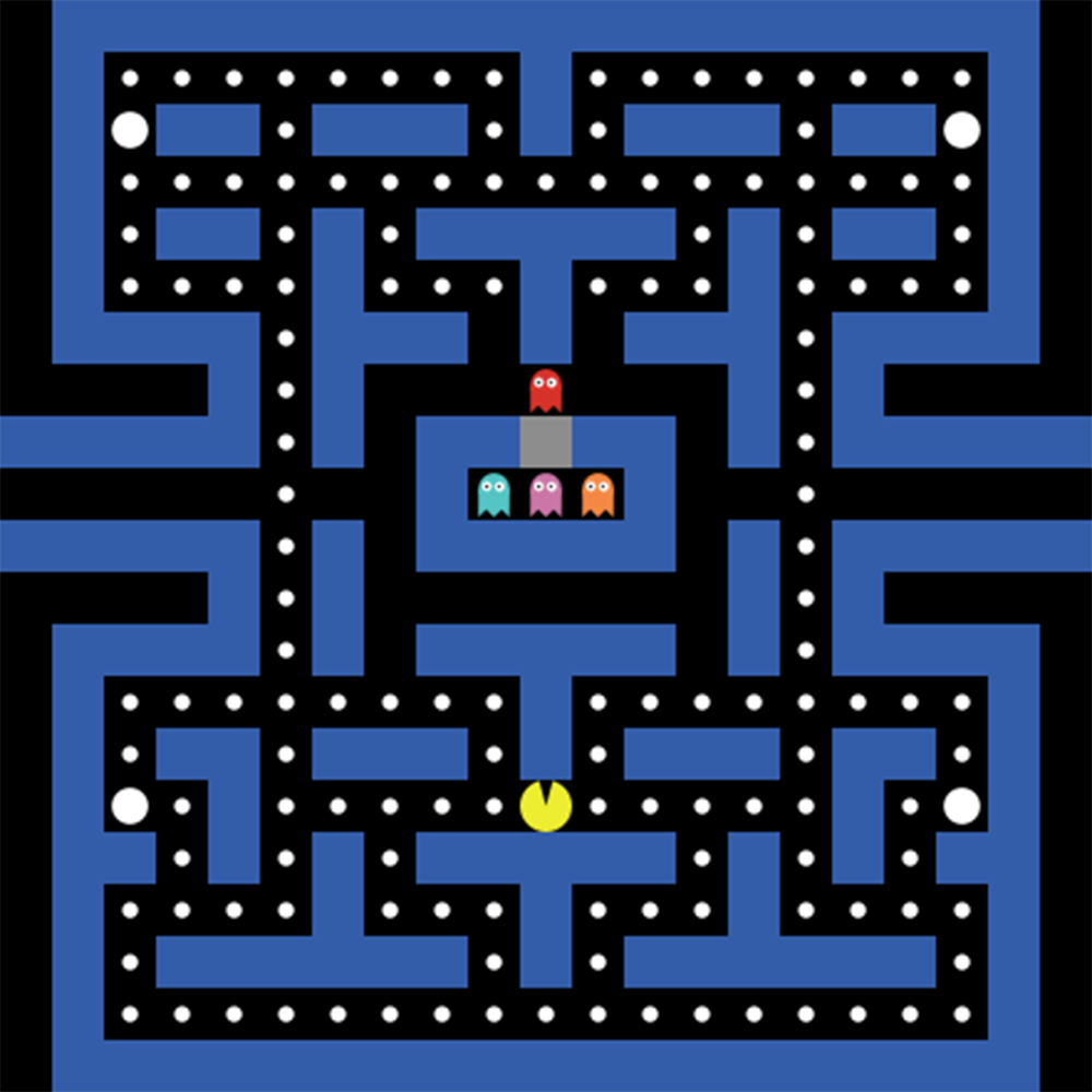
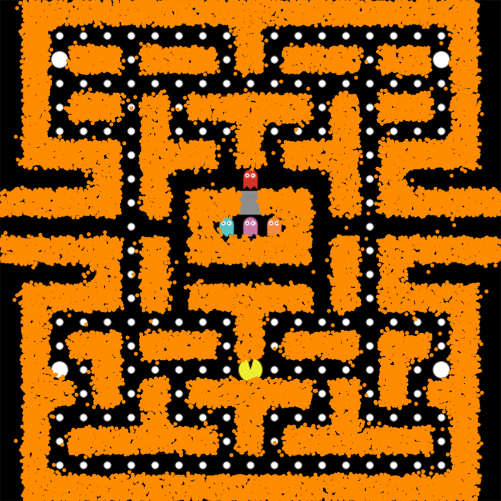
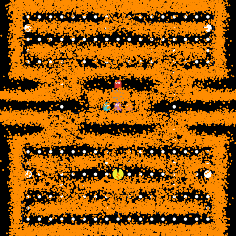
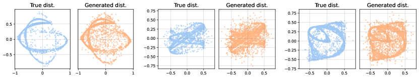
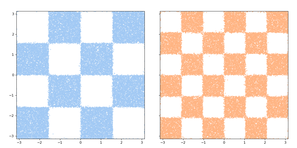
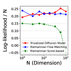
Complicated and High dimensional Torus Data: Our initial comparison entailed contrasting our model with RFM [5] on intricate datasets such as the checkerboard and Pacman on $\mathbb{T}^{2}$, which are discontinuous and multi-modal. Here, Pacman is a dataset newly curated by us to test generation on torus in challenging situations. It’s noted in Lou et al. [26, Fig.3] that RFM produces less satisfactory results when generating complicated patterns on torus, such as the checkerboard with a size larger than $4\times 4$. We observed that RFM ran into a similar issue when learning the Pacman data, which is arguably more sophisticated. Figure 4 and Figure 2 show that our model consistently exhibited proficiency in generating intricate patterns within the torus manifold. A scalability study shown in Figure 5 confirmed our method’s good scalability to high-dimensional cases with minimal degradation in absolute performance (NLL). For the scalability study, we adopted the same setting considered in RFM and compared with its results.

Figure 5: Log likelihood $(\uparrow)$ v.s. Dimensions.

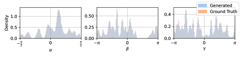
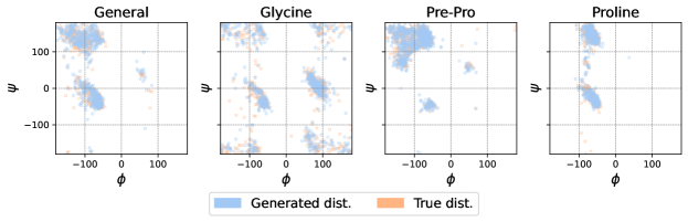
Protein/RNA Torison Angles on Torus: We also test on the popular protein [27] and RNA [32] datasets compiled by Huang et al. [16]. These datasets correspond to configurations of macro-molecules represented by torsion angles (hence non-Euclidean), which are 2D or 7D. Results, including generated data of the protein datasets, are presented in Table 1 and Figure 7. The results of RFM were taken from [5], where RDM was compared to and results of RSGM were not provided. Notably, our model outperforms the baselines by a significant margin, as evidenced by the visualizations of RNA illustrating the alignment of generated data with ground truth via density plots. The empirical results demonstrating our model’s substantial performance gains are possibly rooted in the proposed simulation-free training, high-accuracy sampling, and reduced number of approximations.

Table 1: Test NLL $(\downarrow)$ over Protein/RNA datasets

Model	General (2D)	Glycine (2D)	Proline (2D)	Pre-Pro (2D)	RNA (7D)
Dataset size	138208	13283	7634	6910	9478
RDM [16]	$1.04\pm 0.012$	$1.97\pm 0.012$	$0.12\pm 0.011$	$1.24\pm 0.004$	$-3.70\pm 0.592$
RFM [5]	$1.01\pm 0.025$	$1.90\pm 0.055$	$0.15\pm 0.027$	$1.18\pm 0.055$	$-5.20\pm 0.067$
TDM	$\mathbf{0.69\pm 0.14}$	$\mathbf{1.04\pm 0.27}$	$\mathbf{-0.60\pm 0.15}$	$\mathbf{0.52\pm 0.10}$	$\mathbf{-6.86\pm 0.46}$

Model	Log likelihood
RSGM [16]	$0.20\pm 0.03$
TDM	$\mathbf{0.292\pm 0.07}$

Figure 6: Log likelihood and visualization of generated data for $\mathsf{SO}(3)$ with $32$ mixture components.

Figure 7: Visualization of Generated Protein Torsion Angle

Special Orthogonal Group in High Dimensions: We now evaluate our model’s performance on $\mathsf{SO}(n)$ data. Notably, our model is the first reported one to successfully generate beyond $n=3$. For $\mathsf{SO}(3)$, we generate a difficult mixture distribution in the same way as in [8]. We also generate data for $\mathsf{SO}(n)$ with $n>3$ in a similar fashion. With trivialization technique, we bypass the need to compute the Riemannian logarithm map used in RFM training or eigenfunctions of the heat kernel on $\mathsf{SO}(n)$, which is needed by RSGM [8] but in general does not admit a tractable form. The accuracy of our approach can be seen from both the visualization and NLL metric in Figure 6 and Figure 1.

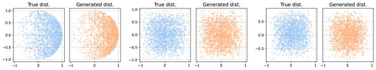
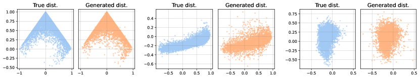
Learning Time-Evolution Operators for an Ensemble of Quantum Systems: Lastly, we experiment with a complex-valued Lie group, the unitary group $\mathsf{U}(n)$. $\mathsf{U}(n)$ holds critical importance in, e.g., high energy physics [44] and quantum sciences [34]. Our approach, arguably for the first time, tackles the generative modeling of $\mathsf{U}(n)$ data and manages to scale to nontrivial dimensions. Specifically, how quantum system evolves is encoded by a unitary operator, i.e. an element in $\mathsf{U}(n)$, and we consider training data corresponding to an ensemble of quantum systems, and aim at generating more quantum systems that are similar. Two examples are tested, respectively quantum oscillators in random potentials, and Transverse Field Ising Model with random couplings and field strength. (Spatial discretization, if needed, of) the time evolution operator of Schrödinger equation for each system gives one $\mathsf{U}(n)$ data point in the training set. Fig.3 provides marginals’ scatter plots to showcase the fidelity of our generated distributions, for Quantum Oscillators. Fig.8 is for Transverse Field Ising Model.

Figure 8: Visualization of Generated Time-evolution Operator of Transverse Field Ising Model on $\mathsf{U}(n)$. $\textbf{Left: }\mathsf{U}(4)$. $\textbf{Middle: }\mathsf{U}(8)$. $\textbf{Right: }\mathsf{U}(8)$

5 Limitation and Future Possibilities

The technique of trivialization does not work for general manifolds, although it is possible to extend our approach to homogeneous spaces. Meanwhile, there is significant potential for improvement in the training procedure, including the adoption of techniques such as preconditioning and exponential moving average tuning from EDM [18]. In addition, network architecture has not been the focus of investigation in this work, but we anticipate quantum data, for example, would benefit from specialized score parametrization other than U-Net, which suits images better.

Appendix A Backgrounds

Diffusion Generative Model in Euclidean spaces: We first review Diffusion Generative Models (sometimes also referred to as Score-based Generative Model, denoising diffusion model, etc.) [15, 40]. Here, we adopt the Stochastic Differential Equations (SDE) description [40]. Given samples of $\mathbb{R}^{d}$-valued random variable $X_{0}$ that follows the data distribution $p_{0}$ which we are interested in, denoising diffusion adopts a forward noising process followed by a backward denoising generation process to generate more samples of $p_{0}$. The forward process transports the data distribution to a known, easy-to-sample distribution by evolving the initial condition via an SDE,

$$\mathrm{d}X_{t}=f(X_{t},t)\mathrm{d}t+\sqrt{2\gamma(t)}\mathrm{d}W_{t},\quad X_{0}\sim p_{0}.$$ (13)

In this case, $p_{+\infty}$ will be a standard Gaussian $\mathcal{N}(0,I)$ with appropriate choice of $\gamma(t)$. The backward process then utilizes the time-reversal of the SDE (13) [2]. More precisely, if one considers

$$\mathrm{d}Y_{t} =\big{(}-f(Y_{t},t)+2\gamma(t)\nabla\log p_{T-t}(Y_{t})\big{)}{\mathrm{d}}t+\sqrt{2\gamma(T-t)}\mathrm{d}W_{t},\quad Y_{0}\sim p_{T}.$$ (14)

Then we have $Y_{t}\sim p_{T-t}$, i.e. $Y_{t}=X_{T-t}$ in distribution. In particular, the $T$-time evolution of (14), $Y_{T}$, will follow the data distribution $p_{0}$. In practice, one considers evolving the forward dynamics for finite but large time $T$, so that $p_{T}\approx\mathcal{N}(0,I)$, and then initialize the backward dynamics using $Y_{0}\sim\mathcal{N}(0,I)$ and simulate it numerically till $t=T$ to obtain approximate samples of the data distribution. Critically, the score function $s$ needs to be estimated in the forward process.

To do so, the score $\nabla\log p_{t}$ is often approximated using a neural network $s_{\theta}$. For linear forward SDE, it is typically trained by minimizing an objective based on denoising score matching [43], namely

$$\mathbb{E}_{t}\mathbb{E}_{X_{0}\sim p_{0}}\mathbb{E}_{X_{t}\sim p_{t}(\cdot|X_{0})}\|s_{\theta}(X_{t},t)-\nabla\log p_{t}(X_{t}|X_{0})\|^{2}$$ (15)

where $\nabla\log p_{t}(X_{t}|X_{0})$ is the conditional score derived from the solution of (13) with a given initial condition.

Kinetic Langevin dynamics in Euclidean spaces, and CLD: When Einstein first proposed ‘Brownian motion’, he actually thought of a mechanical system under additional perturbations from noise and friction [12]. This is now (generalized, formalized, and) known as the kinetic Langevin dynamics [e.g., 33], i.e.

$$\begin{cases}dQ&=M^{-1}Pdt\\ dP&=-\gamma Pdt-\nabla V(Q)dt+\sigma dW_{t}\end{cases}$$ (16)

which converges, as $t\to\infty$, to a limiting probability distribution $Z^{-1}\exp(-(P^{T}M^{-1}P/2+V(Q))/T)dPdQ$ under mild conditions, where $M$ is mass matrix that can be assumed to be $I$ without loss of generality, and $T=\sigma^{2}/(2\gamma)$ is known as the temperature. If $T$ is fixed and $\gamma\to\infty$, one recovers (in distribution and after time rescaling) overdamped Langevin dynamics

$$dQ=-\nabla V(Q)dt+\sqrt{2T}dW_{t}.$$

Just like how overdamped Langevin (often with $V$ being quadratic) can be used as the forward process for diffusion generative model, kinetic Langevin can also be used as the forward process. In fact, in a seminal paper, Dockhorn et al. [11] used it to smartly bypass the singularity of score function at $t=0$ when overdamped Langevin is employed as the forward process and data is supported on a low dimensional manifold, and called the resulting method CLD. Similar to Equation 14, one can construct the reverse process of Equation 16 as follow,

$$\begin{cases}dQ&=-M^{-1}Pdt\\ dP&=\gamma Pdt+\nabla V(Q)dt+\sigma^{2}\nabla_{P}\log p(Q,P,t){\mathrm{d}}t+\sigma dW_{t}.\end{cases}$$ (17)

By endowing $P$ with Gaussian initial condition, $p$ is fully supported in $P$ space, and since the score function only takes the gradient with respect to $P$, it no longer has the aforementioned singularity issue when $t$ tends to zero. This benefits score parameterization and learning.

Finally, let us contrast the trivialized Lie group kinetic Langevin dynamics (used as forward dynamics in this work) with the classical Euclidean kinetic Langevin dynamics by setting $\sigma=\sqrt{2\gamma}$ and $M=1$:

$$\text{Lie:}\begin{cases}\dot{g}=g\xi,\\ {\mathrm{d}}\xi=-\gamma\xi{\mathrm{d}}t-T_{g}\mathsf{L}_{g^{-1}}(\nabla U(g)){\mathrm{d}}t+\sqrt{2\gamma}{\mathrm{d}}W_{t}^{\mathfrak{g}},\end{cases}\text{Euclidean:}\begin{cases}\dot{Q}=P,\\ {\mathrm{d}}P=-\gamma P{\mathrm{d}}t-\nabla U(Q){\mathrm{d}}t+\sqrt{2\gamma}{\mathrm{d}}W_{t},\end{cases}$$

Note the main difference is the 1st line, i.e. the position dynamics; the 2nd line is identical except for conservative forcing, but that has to be different in the manifold case.

Lie group: A Lie group is a differentiable manifold that also has a group structure, denoted by $G$. A Lie algebra is a vector space with a bilinear, alternating binary operation that satisfies the Jacobi identity, known as the Lie bracket. The tangent space of a Lie group at $e$ (the identity element of the group) is a Lie algebra, denoted as $\mathfrak{g}:=T_{e}G$.

Appendix B Time Reversal Formula

In this section, we will prove the time reversal formula stated in Theorem 1. We first introduce an important lemma and calculate the adjoint of the infinitesimal generator of a general diffusion process. We then apply the lemma to derive the Fokker-Planck equation for our process of interest and finish the proof.

Lemma 1.

Given $\alpha,\beta:G\times\mathfrak{g}\to\mathfrak{g}$, let $\mathcal{L}$ denote the infinitesimal generator of the following dynamic

$$\begin{cases}\dot{g}=T_{e}L_{g}\alpha(g,\xi){\mathrm{d}}t\\ {\mathrm{d}}\xi=\beta(g,\xi){\mathrm{d}}t+\sqrt{2\gamma(t)}{\mathrm{d}}W_{t}\end{cases}$$ (18)

The adjoint of $\mathcal{L}$ is given by

$$\mathcal{L}^{*}p =-\operatorname{div}_{g}(pT_{e}L_{g}\alpha)-\operatorname{div}_{\xi}(p\beta)+\gamma(t)\Delta_{\xi}p$$

Proof of Lemma 1.

We first write down the infinitesimal generator $\mathcal{L}$ for SDE (18). For any $f\in C_{0}^{2}(G\times\mathfrak{g})$, $\mathcal{L}$ is defined as

$$\mathcal{L}f(g,\xi):= \lim_{\delta\rightarrow 0}\frac{\mathbb{E}\left[f(g_{\delta},\xi_{\delta})|(g_{0},\xi_{0})=(g,\xi)\right]-f(g,\xi)}{\delta}$$

$$= {\left\langle\nabla_{g}f,T_{e}L_{g}\alpha\right\rangle}+{\left\langle\nabla_{\xi}f,\beta\right\rangle}+\gamma(t)\Delta_{\xi}f$$

By definition, $\mathcal{L}^{*}:C^{2}\rightarrow C^{2}$ (the adjoint operator of $\mathcal{L}$) satisfies $\int_{G\times\mathfrak{g}}p\mathcal{L}f{\mathrm{d}}g{\mathrm{d}}\xi=\int_{G\times\mathfrak{g}}f\mathcal{L}^{*}p\,{\mathrm{d}}g{\mathrm{d}}\xi$ for any $f,p\in C_{0}^{2}(G\times\mathfrak{g})$. By the divergence theorem, we have

$$\int_{G\times\mathfrak{g}}p\mathcal{L}f\,{\mathrm{d}}g{\mathrm{d}}\xi=\int_{G\times\mathfrak{g}}f\big{(}-\operatorname{div}_{g}(pT_{e}L_{g}\alpha)-\operatorname{div}_{\xi}(p\beta)+\gamma(t)\Delta_{\xi}p\big{)}\,{\mathrm{d}}g{\mathrm{d}}\xi$$

Here $T_{e}L_{g}\xi$ stands for the left-invariant vector filed on $G$ generated by $\xi\in\mathfrak{g}$. As a result, we have

$$\mathcal{L}^{*}p =-\operatorname{div}_{g}(pT_{e}L_{g}\alpha)-\operatorname{div}_{\xi}\left(p\beta\right)+\gamma(t)\Delta_{\xi}p$$

∎

We are now ready to show that the backward dynamic (5) is the time reversal process of the forward dynamic (1). Fokker-Planck characterizes the evolution of the density of a a stochastic process: denote the density at time $t$ as $\rho_{t}$, we have $\rho_{t}$ satisfies $\frac{\partial}{\partial t}\rho_{t}=\mathcal{L}^{*}\rho_{t}$. Thm. 1 is proved by comparing the Fokker-Planck equation for Eq. (1) and (5).

Proof of Theorem 1.

By denoting the density for SDE following the forward dynamic (1) as $p_{t}$ and the density for SDE following backward dynamic (5) as $\tilde{p}_{t}$, we only need to prove $p_{t}\equiv\tilde{p}_{T-t}$.

Using Lemma 1, the Fokker-Planck equation of the forward dynamic Eq. (1) is given by,

$$\frac{\partial}{\partial t}p_{t}=-\operatorname{div}_{g}(p_{t}T_{e}L_{g}\xi)+\gamma(t)\operatorname{div}_{\xi}(p_{t}\xi)+\gamma(t)\Delta_{\xi}p_{t}$$

and the Fokker-Planck equation for Eq. (5) is given by

$$\frac{\partial}{\partial t}\tilde{p}_{t} =-\operatorname{div}_{g}(-\tilde{p}_{t}T_{e}L_{g}\xi)-2\gamma\operatorname{div}_{\xi}\left(\tilde{p}_{t}\nabla_{\xi}\log\tilde{p}_{t}\right)-\gamma(T-t)\operatorname{div}_{\xi}(\tilde{p}_{t}\xi)+\gamma(T-t)\Delta_{\xi}\tilde{p}_{t}$$

$$=\operatorname{div}_{g}(\tilde{p}_{t}T_{e}L_{g}\xi)-\gamma(T-t)\operatorname{div}_{\xi}(\tilde{p}_{t}\xi)-\gamma(T-t)\Delta_{\xi}\tilde{p}_{t}$$

where the last equation holds due to $\operatorname{div}_{\xi}\left(\tilde{p}_{t}\nabla_{\xi}\log\tilde{p}_{t}\right)=\operatorname{div}_{\xi}\left(\nabla_{\xi}\tilde{p}_{t}\right)=\Delta_{\xi}p_{t}$.
We can calculate the partial derivative of the reversed distribution $\tilde{p}_{T-t}$ with respect to $t$, which gives

$$\frac{\partial}{\partial t}\tilde{p}_{T-t} =-\operatorname{div}_{g}(\tilde{p}_{t}T_{e}L_{g}\xi)+\gamma(t)\operatorname{div}_{\xi}(\tilde{p}_{t}\xi)+\gamma(t)\Delta_{\xi}\tilde{p}_{t}$$

Note that this exactly matches the expression for $\frac{\partial}{\partial t}p_{t}$. Together with the same initial condition $\tilde{p}_{0}=p_{T}$, we deduce that $p_{t}\equiv\tilde{p}_{T-t}$ for all $t$. ∎

Appendix C Denoising Score Matching for Abelian Lie group

We first state a detailed version of Theorem 2 in the following,

Corollary 1 (Conditional transition probability for Abelian Lie Group).

Let $G$ be an Abelian Lie group which is isomorphic to $\mathbb{T}$ or $\mathsf{SO}(2)$. In this case, the conditional transition probability can be written explicitly as,

$$p_{t|0}(g_{t},\xi_{t}\mid g_{0},\xi_{0})=\operatorname{WN}(\operatorname{logm}(g_{0}^{-1}g_{t});\mu_{g},\sigma^{2}_{g})\cdot\mathcal{N}(\xi_{t};\mu_{\xi},\sigma^{2}_{\xi})$$ (19)

where $\operatorname{WN}(x;\mu,\sigma^{2})$ is the density of the Wrapped Normal distribution with mean $\mu$ and variance $\sigma^{2}$ evaluate at $x$, $\operatorname{logm}$ is the matrix logarithm with principal root, and $\mu_{g},\mu_{\xi},\sigma^{2}_{g},\sigma^{2}_{\xi}$ are are given by,

$$\mu_{g}=\frac{1-e^{-t}}{1+e^{-t}}(\xi_{t}+\xi_{0}),\;\mu_{\xi}=e^{-t}\xi_{0}$$

$$\sigma_{g}^{2}=2t+\frac{8}{e^{t}+1}-4,\;\sigma_{\xi}^{2}=1-e^{-2t}$$

In this section, we will prove Theorem 2 by proving its detailed version in Corollary 1, under the condition that $G$ is an Abelian Lie group which is isomorphic to $\mathbb{T}$ or $\mathsf{SO}(2)$. Note that this allows us to compute the conditional transition probability for $G$ that is also direct product of these Lie groups. The reason is that, for a Lie group $G$ that is a direct product of $\mathbb{T}$ and $\mathsf{SO}(2)$, we can represent an element in $G$ as $(g^{1},\dots,g^{k})$ where $g^{i}\in\mathbb{T}$ or $\mathsf{SO}(2)$. The corresponding Lie Algebra can be represented as $(\xi^{1},\dots,\xi^{k})$. For each $1\leq i\leq k$, $(g^{i},\xi^{i})$, they follow the following dynamic,

$$\begin{cases}\dot{g^{i}_{t}}=g_{t}\xi^{i}_{t},\\ {\mathrm{d}}\xi^{i}_{t}=-\gamma\xi_{t}{\mathrm{d}}t+\sqrt{2\gamma}{\mathrm{d}}W^{i}_{t}\\ g^{i}(0)=g^{i}_{0},\;\xi^{i}(0)=\xi_{0}^{i}\end{cases}$$ (20)

Note that this will not create any confusion since $\xi^{i}\in\mathbb{R}$ and there’s no need for another superscript to indicate other elements in $\xi^{i}$. Moreover, an important consequence of the factorization of the dynamic of $(g,\xi)$ as $k$ independent smaller dynamic is that we can also factorize the conditional transition probability for $g,\xi$ as a product of $k$ conditional transition probability, each computed from $g^{i},\xi^{i}$. This means the following,

$$p_{t|0}(g_{t},\xi_{t}\mid g_{0},\xi_{0})=\prod_{i=1}^{k}p_{t|0}(g^{i}_{t},\xi^{i}_{t}\mid g^{i}_{0},\xi^{i}_{0})$$ (21)

Based on (21), we manage to compute the conditional transition probability of any general connected compact Abelian Lie group, since they are necessarily isomorphic to a power of $\mathbb{T}$ or $\mathsf{SO}(2)$[19]. Therefore, we just need to compute the conditional transition probability for such a base case, which is stated in Theorem 2.

From now on, we will consider $\gamma=1$ for simplicity. Generalization of our results to time-dependent is straightforward. Let’s stick to the notation that $g_{0}\in\mathsf{SO}(2)$, $\xi_{0}\in\mathbb{R}\cong\mathfrak{so}(2)$. We slightly abuse the notation in the sense that, when considering the dynamic for $\xi$, we are considering a valid SDE on $\mathbb{R}$, while when we are considering the dynamic for $g$, $\xi$ should be understood as its matrix representation in $\mathfrak{so}(2)$, which is a $2\times 2$ skew-symmetric matrix. Let also denote $Y_{t}=\int_{0}^{t}\xi_{s}{\mathrm{d}}s$ for notational simplicity.

Since $G$ is Abelian, $[\xi,\hat{\xi}]=0$ for any $\xi,\hat{\xi}\in\mathfrak{g}$, the Magnus series $\Omega_{k}(t)=0$ in (9) for $k\geq 2$, and the solution to the IVP can be written explicitly as,

$$\begin{cases}g_{t}=g_{0}\operatorname{expm}(Y_{t})\\ \xi_{t}=e^{-t}\xi_{0}+\sqrt{2}\int_{0}^{t}e^{-(t-s)}{\mathrm{d}}W_{s}\end{cases}$$ (22)

Notice that $(g_{t},\xi_{t})$ is a push forward of $(\xi_{t},Y_{t})$. Therefore, to find the condition transition $p_{t|0}(g_{t},\xi_{t}\mid g_{0},\xi_{0})$, we first compute the joint distribution of $(\xi_{t},Y_{t})$ conditioned on the $(g_{0},\xi_{0})$, and derive the desired conditional transition probability by computing the probability change of variable.

Since $Y_{t}$ is the time integral of $\xi_{t}$, $(\xi_{t},Y_{t})$ is a Gaussian process, with mean and covariance stated in the following Lemma,

Lemma 2.

For a given $t$, $(\xi_{t},Y_{t})$ is distributed according to a bivariate Gaussian,

$$\begin{pmatrix}\xi_{t}\\ Y_{t}\end{pmatrix}\sim\mathcal{N}\left(\begin{pmatrix}e^{-t}\xi_{0}\\ (1-e^{-t})\xi_{0}\end{pmatrix},\begin{pmatrix}1-e^{-2t}&e^{-2t}(e^{t}-1)^{2}\\ e^{-2t}(e^{t}-1)^{2}&4e^{-t}-e^{2t}+2t-3\end{pmatrix}\right)$$ (23)

Proof of Lemma 2.

To show that the joint distribution $(\xi_{t},Y_{t})$ as the desired expression, we just need to compute the mean and variance of $\xi_{t}$ and $Y_{t}$ respectively, as well as their covariance. For $\xi_{t}$,

$$\mathbb{E}[\xi_{t}]=\mathbb{E}\Big{[}e^{-t}\xi_{0}+\sqrt{2}\int_{0}^{t}e^{-(t-s)}{\mathrm{d}}W_{s}\Big{]}=e^{-t}\xi_{0}$$

$$\operatorname{Var}(\xi_{t})=\operatorname{Var}\Big{(}\sqrt{2}\int_{0}^{t}e^{-(t-s)}{\mathrm{d}}W_{s}\Big{)}=2\int_{0}^{t}e^{-2(t-s)}{\mathrm{d}}s=1-e^{-2t}$$

For $Y_{t}$, since it’s the integration of $\xi_{t}$, it has the following expression,

$$Y_{t} =\int_{0}^{t}e^{-s}\xi_{0}{\mathrm{d}}s+\sqrt{2}\int_{0}^{t}\int_{0}^{p}e^{-(p-s)}{\mathrm{d}}W_{s}{\mathrm{d}}p$$

$$=(1-e^{-t})\xi_{0}+\sqrt{2}\int_{0}^{t}\int_{s}^{t}e^{-(p-s)}{\mathrm{d}}p{\mathrm{d}}W_{s}$$

$$=(1-e^{-t})\xi_{0}+\sqrt{2}\int_{0}^{t}(1-e^{-(t-s)}){\mathrm{d}}W_{s}$$

where we use Stochastic Fubini’s theorem to exchange the integration order of ${\mathrm{d}}W_{s}$ and ${\mathrm{d}}p$. Therefore, we can compute the mean and variance of $Y_{t}$,

$$\mathbb{E}[Y_{t}]=\mathbb{E}\Big{[}(1-e^{-t})\xi_{0}+\sqrt{2}\int_{0}^{t}(1-e^{-(t-s)}){\mathrm{d}}W_{s}\Big{]}=(1-e^{-t})\xi_{0}$$

$$\operatorname{Var}(Y_{t})=\operatorname{Var}\Big{(}\sqrt{2}\int_{0}^{t}(1-e^{-(t-s)}){\mathrm{d}}W_{s}\Big{)}=2\int_{0}^{t}(1-e^{-(t-s)})^{2}{\mathrm{d}}s=4e^{-t}-e^{2t}+2t-3$$

Finally, we need to compute $\operatorname{Cov}(\xi_{t},Y_{t})$ to complete the proof, where we use Ito’s isometry,

$$\operatorname{Cov}(\xi_{t},Y_{t}) =\mathbb{E}\Big{[}2\int_{0}^{t}e^{-(t-s)}{\mathrm{d}}W_{s}\cdot\int_{0}^{t}(1-e^{-(t-s)}){\mathrm{d}}W_{s}\Big{]}$$

$$=2\int_{0}^{t}e^{-(t-s)}\cdot(1-e^{-(t-s)}){\mathrm{d}}s=e^{-2t}(e^{t}-1)^{2}$$

∎

As a corollary of Lemma 2, we can compute the conditional distribution $Y_{t}|\xi_{t}$, here we omit the dependence on $\xi_{0},g_{0}$ for simplicity since all probability considered in this section is conditioned on these two value. The conditional distribution between bivariate Gaussian is equivalent to orthogonal projections,

Corollary 2.

For a give $t$, $Y_{t}|\xi_{t}$ has distribution

$$Y_{t}|\xi_{t}\sim\mathcal{N}\Big{(}\frac{1-e^{-t}}{1+e^{-t}}(\xi_{t}+\xi_{0}),2t+\frac{8}{e^{t}+1}-4\Big{)}$$ (24)

Proof.

Let $\boldsymbol{\Sigma}$ and $\boldsymbol{\mu}$ denotes the variance matrix and the mean vector of $(\xi_{t},Y_{t})$. The $Y_{t}|\xi_{t}$ has conditional mean and variance given by,

$$\mathbb{E}[Y_{t}|\xi_{t}]=\boldsymbol{\mu}_{Y}+\boldsymbol{\Sigma}_{Y\xi}\boldsymbol{\Sigma}_{\xi\xi}^{-1}(\xi_{t}-\boldsymbol{\mu}_{\xi})$$

$$\operatorname{Var}[Y_{t}|\xi_{t}]=\boldsymbol{\Sigma}_{YY}-\boldsymbol{\Sigma}_{Y\xi}\boldsymbol{\Sigma}_{\xi\xi}^{-1}\boldsymbol{\Sigma}_{\xi Y}$$

Plug in the expression for $\boldsymbol{\Sigma}$ and $\boldsymbol{\mu}$, and the expressions simplify to the desired ones. ∎

We need the distribution of $Y_{t}|\xi_{t}$ due to the following factorization of $p_{t|0}(g_{t},\xi_{t}\mid g_{0},\xi_{0})$,

$$p_{t|0}(g_{t},\xi_{t}\mid g_{0},\xi_{0})=p_{t|0}(g_{t}\mid\xi_{t},g_{0},\xi_{0})\cdot p_{t|0}(\xi_{t}\mid g_{0},\xi_{0})$$

Here $p_{t|0}(\xi_{t}\mid g_{0},\xi_{0})$ is known due to $\xi_{t}$ being a Gaussian, we need to compute $p_{t|0}(g_{t}\mid\xi_{t},g_{0},\xi_{0})$, which is a hard object since it’s a distribution on the Lie group $G$. However, we can derive its expression by computing the push-forward of $Y_{t}|\xi_{t},g_{0},\xi_{0}$ by the exponential map. The following theorem characterizes such a change of measure given by the exponential map of Lie group as the push-forward,

Theorem 3 (Theorem 3.1 in Falosi et al. [13]).

Let $G$ denotes a Lie group and $\mathfrak{g}$ its Lie algebra. Consider a distribution $m$ on $\mathfrak{g}$ with density $r(\xi)$ with respect to the Lebesgue measure on $\mathfrak{g}$, the push-forward of $m$ to $G$, denoted as $\operatorname{exp}_{*}(m)$ is absolutely continuous with respect to the Haar measure on $G$, with density $p(g)$ given by,

$$p(g)=\underset{\xi\in\mathfrak{g}:\,\operatorname{expm}(\xi)=g}{\sum}r(\xi)|J(\xi)|^{-1},\quad g\in G,$$

where $J(\xi)=\operatorname{det}\Big{(}\sum_{k=0}^{\infty}\frac{(-1)^{k}}{(k+1)!}(\operatorname{ad}_{\xi})^{k}\Big{)}$.
Moreover, when $G$ is $\mathsf{SO}(2)$ or $\mathbb{T}$, the scenario simplifies to,

$$J(\xi)=1,\forall\xi\in\mathfrak{g}$$

$$\{\xi\in\mathfrak{g}:\,\operatorname{expm}(\xi)=g\}=\{\xi\in\mathfrak{g}:\,\xi=\operatorname{logm}(g)\pm 2k\pi,k\in\mathbb{Z}\}$$

Since the exponential map is not injective, computing the density of the push-forwarded measure at $g\in G$ requires summing over density at all the pre-images $\xi$ of $g$ in $\mathfrak{g}$ and weighted by the inverse of the Jacobian $|J(\xi)|$. Fortunately, for our considered case, both the pre-images and the Jacobian can be explicitly characterized and computed.

Applying Theorem 3 to our case, where $r$ is the density of $Y_{t}|\xi_{t},g_{0},\xi_{0}$, we derive the following expression for $p_{t|0}(g_{t}\mid\xi_{t},g_{0},\xi_{0})$,

$$p_{t|0}(g_{t}\mid\xi_{t},g_{0},\xi_{0})=\sum_{k=-\infty}^{\infty}p_{Y_{t}|\xi_{t}}\big{(}\operatorname{logm}(g_{0}^{-1}g_{t})+2k\pi\big{)}$$ (25)

where $p_{Y_{t}|\xi_{t}}$ denotes the density of $Y_{t}|\xi_{t}$, which is the density of a Gaussian with mean and variance defined in (24). This is also known as the Wrapped Normal distribution [29], its name comes from the fact that the density is generated by "wrapping a distribution" on a circle. Therefore, we denote such a distribution with notation $\operatorname{WN}(x;\mu,\sigma^{2})$ denotes such as density evaluated at point $x$, where $\mu,\sigma^{2}$ is the mean and variance of the normal distribution being wrapped. This finishes the proof of Theorem 2 and Corollary 1.

Appendix D Proability Flow ODE and Operator Splitting Integrator

In this section, we will first discuss in detail the Operator Splitting Integrator (OSI) and how they help integrate the forward and backward trivialized kinetic dynamics accurately in a manifold-preserving, projection-free manner. We then introduce the probability flow ODE of the backward dynamic, which is an ODE that is marginally equivalent to dynamic (5). We will also introduce the OSI for the probability flow ODE.

D.1 Operator Splitting Integrator

In this section, we will demonstrate how OSIs are constructed from the dynamics and the benefits they enjoy. We restrict our attention to first-order numerical integrators in the following discussion. However, such an approach can be generalized and we can indeed craft an OSI with arbitrary order of accuracy by following the approach in Tao and Ohsawa [41].

Forward Integrator: Recall that the forward dynamic (3) can be split into two smaller dynamics,

$$\begin{array}[]{ccc}A^{\mathcal{F}}_{g}:\Big{\{}\begin{array}[]{ll}\dot{g_{t}}=g_{t}\xi_{t}\\ {\mathrm{d}}\xi_{t}=0\,{\mathrm{d}}t\end{array}&+&A^{\mathcal{F}}_{\xi}:\Big{\{}\begin{array}[]{ll}\dot{g_{t}}=0\\ {\mathrm{d}}\xi_{t}=-\gamma\xi_{t}{\mathrm{d}}t+\sqrt{2\gamma}{\mathrm{d}}W^{\mathfrak{g}}_{t}\end{array}\end{array}$$

While the original dynamic does not admit a simple closed-form solution, $A^{\mathcal{F}}_{g}$ and $A^{\mathcal{F}}_{\xi}$ can be solved explicitly as is shown in the following equations,

$$A^{\mathcal{F}}_{g}:\;g(t)=g(0)\operatorname{expm}(t\xi(0)),\;\xi(t)=\xi(0)$$

$$A^{\mathcal{F}}_{\xi}:\;g(t)=g(0),\xi(t)=\exp(-\gamma t)\xi(0)+\int_{0}^{t}\sqrt{2\gamma}\exp(-\gamma(t-s)){\mathrm{d}}W_{s}^{\mathfrak{g}}$$

Therefore, we can integrate $A^{\mathcal{F}}_{g}$ and $A^{\mathcal{F}}_{\xi}$ alternatively for each timestep $h$ in order to integrate the original forward dynamic. The detailed algorithm can be found in Algorithm 2.

Backward Integrator: Recall that the backward dynamic (12) can be split into two smaller dynamics,

$$\begin{array}[]{ccc}A^{\mathcal{B}}_{g}:\Big{\{}\begin{array}[]{ll}\dot{g_{t}}=-g_{t}\xi_{t}\\ {\mathrm{d}}\xi_{t}=0\,{\mathrm{d}}t\end{array}&+&A^{\mathcal{B}}_{\xi}:\Big{\{}\begin{array}[]{ll}\dot{g_{t}}=0\\ {\mathrm{d}}\xi_{t}=\gamma\xi_{t}{\mathrm{d}}t+2\gamma s_{\theta}(g_{t},\xi_{t},t){\mathrm{d}}t+\sqrt{2\gamma}{\mathrm{d}}W^{\mathfrak{g}}_{t}\end{array}\end{array}$$

Again, we can write out explicit solutions to $A^{\mathcal{B}}_{g}$ and $A^{\mathcal{B}}_{\xi}$ in the following equations,

$$A^{\mathcal{B}}_{g}:\;g(t)=g(0)\operatorname{expm}(-t\xi(0)),\;\xi(t)=\xi(0)$$

$$A^{\mathcal{B}}_{\xi}:\;g(t)=g(0),\xi(t)=\exp(\gamma t)\xi(0)+\int_{0}^{t}\sqrt{2\gamma}\exp(\gamma(t-s)){\mathrm{d}}W_{s}^{\mathfrak{g}}+2\gamma\int_{0}^{t}\exp(\gamma(t-s))s_{\theta}(g_{s},\xi_{s},s){\mathrm{d}}s$$

Note that, the solution to $A^{\mathcal{F}}_{\xi}$, though presented in an explicit form, can’t be implemented in practice since we can not integrate exactly the neural network $s_{\theta}$. We employ an approximation here and discretize the nonlinear component $s_{\theta}$ by using a left-point rule, i.e. pretending that $g$ and $\xi$ do not change over a short time $h$, and still use the exponential integration technique to conduct the exact integration of the rest of the linear dynamic. The detailed algorithm can be found in Algorithm 3.

Algorithm 2 Forward Operator Splitting Integration (FOSI)

1:step size $h$, total steps $N$, friction constant $\gamma>0$, initial condition $\bar{g}\in G,\bar{\xi}\in\mathfrak{g}$

2:Set $g_{0}=\bar{g},\xi_{0}=\bar{\xi}$

3:for $n=1,\dots,N$ do

4:     Sample i.i.d. $\epsilon_{n-1}^{i}\sim\mathcal{N}(0,1-\exp(-2\gamma h)$ for $1\leq i\leq\operatorname{dim}g$

5:     $\xi^{i}_{n}=\exp(-\gamma h)\xi^{i}_{n-1}+\epsilon_{n-1}^{i}$ $\triangleright$ Entrywise exponential integration for $\xi$

6:     $g_{n}=g_{n-1}\operatorname{expm}(h\xi_{n})$ $\triangleright$ Lie group preserving update for $g$

7:end for

8:return $\{g_{k},\xi_{k}\}_{k=0,\dots,N}$ $\triangleright$ Return whole trajectory

Algorithm 3 Backward Operator Splitting Integration (BSOI)

1:step size $h$, total steps $N$, friction constant $\gamma>0$, score network $s_{\theta}$, initial condition $\bar{g}\in G,\bar{\xi}\in\mathfrak{g}$

2:Set $g_{0}=\bar{g},\xi_{0}=\bar{\xi}$

3:for $n=1,\dots,N$ do

4:     Set $\boldsymbol{s}_{n-1}=s_{\theta}(g_{n-1},\xi_{n-1},(n-1)h)$

5:     Sample i.i.d. $\epsilon^{i}_{n-1}\sim\mathcal{N}(0,\exp(2\gamma h)-1)$ for $1\leq i\leq\operatorname{dim}\mathfrak{g}$

6:     $\xi^{i}_{n}=\exp(\gamma h)\xi^{i}_{n-1}+2(\exp(\gamma h)-1)s_{n-1}^{i}+\epsilon^{i}_{n-1}$ $\triangleright$ Entrywise exponential integration for $\xi$

7:     $g_{n}=g_{n-1}\operatorname{expm}(-h\xi_{n})$ $\triangleright$ Lie group preserving update for $g$

8:end for

9:return $g_{N},\xi_{N}$ $\triangleright$ Return final iterate

Advantages of OSI: The benefits of using an OSI for integration are threefold.

(1) The first benefit of the OSI is high numerical accuracy. In both the forward and backward dynamic, the linear component of the dynamic is integrated exactly due to the use of the exponential integration technique. This implies that, while OSI is still a first-order method in terms of the order of errors, it enjoys a smaller prefactor thanks to the reduction in error source compared with the Euler–Maruyama method (EM).

(2) The second benefit of OSI is that the trajectories generated stay on the manifold $G\times g$ for the whole time, $(g(kh),\xi(kh))\in G\times\mathfrak{g}$ for any $k\geq 0$. If we use the EM scheme to integrate the Riemannian component of the dynamic, which is the $g$ dynamic, we would arrive at iterates $g((k+1)h)=g(kh)+h\cdot g(kh)\xi(kh)$. Note that since $g(kh)\xi(kh)$ is in the tangent space of Lie group G at point $g(kh)$, moving arbitrary short time $h$ along such direction would result in $g((k+1)h)\notin G$. Therefore, to achieve a valid trajectory on $G$, we need to employ a projection $\pi_{G}$ onto the manifold, which causes additional numerical errors apart from the time discretization error. If employing OSI, we will be free from such a concern of leaving the manifold and also the projection errors.

(3) The third benefit of OSI is that the numerical scheme is projection-free. As we have discussed in point (2), EM method does not respect the Riemannian geometry structure of the Lie group and constantly requires the application of projections to achieve valid iterates. Apart from the numerical error, computing such a projection could be problematic. In general, Lie groups live in a nonconvex set, which naturally raises concerns about the existence of the closed-form formula for such projections and more generally, how to implement them in a fast algorithm. For example, $\mathsf{SO}(n)$ is the set of matrices satisfies $\{X\in\mathbb{R}^{n\times n}\mid X^{\top}X=XX^{\top}=I_{n}\}$, which is characterized by nonlinear constraints. Therefore, finding out the projection onto these Lie groups requires heavy work and needs to be investigated on a case-by-case basis. Not to mention the possibility that these projection functions could be difficult to implement and require heavy computational resources, which is certainly not scalable for large-scale applications and high-dimensional tasks. On the contrary, by employing OSI, we can enjoy a projection-free numerical algorithm and reduce the complexity of both training and generation.

D.2 Probability Flow ODE

In this section, we will introduce the OSI for probability flow ODE. We recall that the probability flow ODE is given by,

$$\begin{cases}\dot{g_{t}}=-g_{t}\xi_{t},\\ {\mathrm{d}}\xi_{t}=\gamma(T-t)\xi_{t}{\mathrm{d}}t+\gamma\nabla_{\xi}\log p_{T-t}(g_{t},\xi_{t}){\mathrm{d}}t\end{cases}$$

Similar to the SDE setting, this can be split into two smaller dynamics,

$$\begin{array}[]{ccc}A^{\mathcal{P}}_{g}:\Big{\{}\begin{array}[]{ll}\dot{g_{t}}=-g_{t}\xi_{t}\\ {\mathrm{d}}\xi_{t}=0\,{\mathrm{d}}t\end{array}&+&A^{\mathcal{P}}_{\xi}:\Big{\{}\begin{array}[]{ll}\dot{g_{t}}=0\\ {\mathrm{d}}\xi_{t}=\gamma\xi_{t}{\mathrm{d}}t+\gamma s_{\theta}(g_{t},\xi_{t},t){\mathrm{d}}t\end{array}\end{array}$$

Similar to the Backward Operator Splitting Integrator (BSOI), we employ an approximation of the $\xi$ dynamic, discretize the nonlinear component $s_{\theta}$ by using a left-point rule, i.e. pretending that $g$ and $\xi$ do not change over a short time $h$, and use the exponential integration technique to conduct the exact integration of the rest of the linear dynamic. The details can be found in Algorithm 4.

Algorithm 4 Probability Flow ODE

1:step size $h$, total steps $N$, friction constant $\gamma>0$, score network $s_{\theta}$, initial condition $\bar{g}\in G,\bar{\xi}\in\mathfrak{g}$

2:Set $g_{0}=\bar{g},\xi_{0}=\bar{\xi}$

3:for $n=1,\dots,N$ do

4:     Set $\boldsymbol{s}_{n-1}=s_{\theta}(g_{n-1},\xi_{n-1},(n-1)h)$

5:     $\xi^{i}_{n}=\exp(\gamma h)\xi^{i}_{n-1}+(\exp(\gamma h)-1)s_{n-1}^{i}$ $\triangleright$ Entrywise exponential integration for $\xi$

6:     $g_{n}=g_{n-1}\operatorname{expm}(-h\xi_{n})$ $\triangleright$ Lie group preserving update for $g$

7:end for

8:return $g_{N},\xi_{N}$ $\triangleright$ Return final iterate

Appendix E Evolution of KL divergence

In this section, we will discuss the effectiveness of likelihood training in terms of learning the correct data distribution. We will show that the KL divergence between the true data distribution $p_{0}$ and the learned data distribution can be bounded by accumulated score-matching errors up to an additional discrepancy error caused by a mismatch in the initial condition.

Recall that $\mathbf{X_{t}}=(g_{t},\xi_{t})$ is the trajectory of the forward dynamics (3), with $\mathbf{X}_{t}$ admitting a smooth density $p_{t}(g_{t},\xi_{t})$ with respect to the product of Haar measure on $G$ and Lebesgue measure on $\mathfrak{g}$. Let’s denote $(q_{t})_{t\in[0,T]}=(p_{T-t})_{t\in[0,T]}$. Note that by construction, $q_{0}=p_{T}\approx\pi^{*}$ when $T$ is large, where $\pi^{*}$ is the invariant distribution of the forward dynamic (3). Also, $q_{T}=p_{0}$ is the initial condition for the forward dynamic, which in practice is the (partially unknown) joint data distribution on $g$ and $\xi$. Recall that we have denoted the sequence of probability distribution $q^{\theta}_{t}$ as the density of $\mathcal{L}(\mathbf{Y}_{t}^{\theta})$ with respect to the reference measure, where $\mathbf{Y}_{t}^{\theta}$ is the trajectory of the learned backward dynamic in (7).

We have Theorem 4 regarding the KL divergence between the learnt data distribution $q_{T}^{\theta}$ and the true data distribution $p_{0}$,

Theorem 4.

Let $\mathbf{Y}_{t}^{\theta}$ be the trajectory of the learnt backward dynamic (7) under initial condition $\mathbf{Y}_{0}^{\theta}=\pi_{*}$, $\mathbf{Y}_{t}^{\theta}$ has density $(q^{\theta}_{t})_{t\in[0,T]}$. When the score is given by $s_{\theta}(g,\xi,t):=\nabla_{\xi}\log\hat{q}_{T-t}(g,\xi,t)$, where $(\hat{q}_{t})_{t\in[0,T]}$ is the density of the forward dynamic (3) under initial condition $\hat{q}_{0}$ and satisfies $\hat{q}_{T}=\pi_{*}$. We then have

$${D_{\operatorname{KL}}\left(p_{0}\parallel q_{T}^{\theta}\right)}=\int_{0}^{T}\int_{G\times\mathfrak{g}}p_{T-t}(g,\xi){\left\|\nabla_{\xi}\log p_{T-t}(g,\xi)-s_{\theta}(g,\xi,t)\right\|}^{2}{\mathrm{d}}g{\mathrm{d}}\xi{\mathrm{d}}t+D_{\operatorname{KL}}(p_{T}\parallel\pi_{*})$$

In order to prove Theorem 4, we need the following Lemma that characterizes the time derivative of the KL divergence between two sequences of probability distributions that corresponds to the time marginal of the same SDE with different initial conditions.

Lemma 3.

Given $p_{0},q_{0}$ two distributions on $G\times g$. We denote the sequence of probability distributions $(p_{t}){t\geq 0}$ and $(q_{t}){t\geq 0}$ the marginals of the forward dynamic (3) with initial conditions $p_{0}$ and $q_{0}$ respectively. Then, $p_{t}$ and $q_{t}$ satisfies

$$\frac{\partial}{\partial t}D_{\operatorname{KL}}(p_{t}\parallel q_{t})=\int_{G\times\mathfrak{g}}\gamma(t)p_{t}{\left\|\nabla_{\xi}\log p_{t}-\nabla_{\xi}\log q_{t}\right\|}^{2}{\mathrm{d}}g{\mathrm{d}}\xi$$

where $\nabla_{\xi}$ is the gradient w.r.t. $\xi$.

Lemma 3 relates the time derivative of KL divergence between two distributions to the difference in their score integrated over the manifold $G\times g$. To prove this lemma, we need to derive the Fokker-Planck equation for $p_{t}$ and $q_{t}$ respectively.

Proof of Lemma 3.

We prove a general case and consider the general form of forward dynamic described in (13). The evolution of $p_{t}$ and $q_{t}$ can be characterized by following Fokker-Plank equations,

$$\frac{\partial}{\partial t}p_{t}=\mathcal{L}^{*,p}p_{t}=-\operatorname{div}_{g}(p_{t}T_{e}L_{g}\xi)+\gamma(t)\left(\operatorname{div}_{\xi}(p_{t}\xi)+\Delta_{\xi}p_{t}\right)$$

$$\frac{\partial}{\partial t}q_{t}=\mathcal{L}^{*,q}q_{t}=-\operatorname{div}_{g}(q_{t}T_{e}L_{g}\xi)+\gamma(t)\left(\operatorname{div}_{\xi}(q_{t}\xi)+\Delta_{\xi}q_{t}\right)$$

where $\operatorname{div}_{g}$ is the divergence of vector fields on $G$ under the left-invariant metric we choose, $\operatorname{div}_{\xi}$ is the divergence in $\mathfrak{g}$ and $\Delta_{\xi}$ is the Laplace operator on $\mathfrak{g}$. They are well-defined since $\mathfrak{g}$ is a linear space. Consequently, we can evaluate the time derivative of KL divergence between $p_{t}$ and $q_{t}$, where the integration is performed over $G\times g$ unless specifically noted,

$$\frac{\partial}{\partial t}D_{\operatorname{KL}}(p_{t}\parallel q_{t}) =\frac{\partial}{\partial t}\Big{(}\int p_{t}\log\frac{p_{t}}{q_{t}}{\mathrm{d}}g{\mathrm{d}}\xi\Big{)}$$

$$=\int\frac{\partial p_{t}}{\partial t}\log\frac{p_{t}}{q_{t}}\,{\mathrm{d}}g{\mathrm{d}}\xi-\int\frac{\partial q_{t}}{\partial t}\frac{p_{t}}{q_{t}}\,{\mathrm{d}}g{\mathrm{d}}\xi$$

$$=\int\left(\log\frac{p_{t}}{q_{t}}\right)\mathcal{L}^{*,p}p_{t}{\mathrm{d}}g{\mathrm{d}}\xi-\int\left(\frac{p_{t}}{q_{t}}\right)\mathcal{L}^{*,q}q_{t}{\mathrm{d}}g{\mathrm{d}}\xi$$

Using the divergence theorem, we have for any smooth function $f:G\times\mathfrak{g}\to\mathbb{R}$, we have

$$\int f\cdot\mathcal{L}^{*,p}p_{t}{\mathrm{d}}g{\mathrm{d}}\xi=\int{\left\langle\nabla_{g}f,p_{t}T_{e}\mathsf{L}_{g}\xi\right\rangle}+{\left\langle\nabla_{\xi}f,p_{t}\gamma(t)\left(\xi+\nabla_{\xi}\log p_{t}\right)\right\rangle}{\mathrm{d}}g{\mathrm{d}}\xi$$

Similar results holds for $\mathcal{L}^{*,q}$. As a consequence, applying the previous equation with $f=\log\frac{p_{t}}{q_{t}}$ and $f=\frac{p_{t}}{q_{t}}$ respectively, we can write,

$$\frac{\partial}{\partial t}D_{\operatorname{KL}}(p_{t}\parallel q_{t}) =\int{\left\langle\nabla_{g}\log\frac{p_{t}}{q_{t}},p_{t}T_{e}\mathsf{L}_{g}\xi\right\rangle}+{\left\langle\nabla_{\xi}\log\frac{p_{t}}{q_{t}},p_{t}\gamma(t)\left(\xi+\nabla_{\xi}\log p_{t}\right)\right\rangle}{\mathrm{d}}g{\mathrm{d}}\xi$$

$$\qquad-\int{\left\langle\nabla_{g}\frac{p_{t}}{q_{t}},q_{t}T_{e}\mathsf{L}_{g}\xi\right\rangle}-{\left\langle\nabla_{\xi}\frac{p_{t}}{q_{t}},q_{t}\gamma(t)\left(\xi+\nabla_{\xi}\log q_{t}\right)\right\rangle}{\mathrm{d}}g{\mathrm{d}}\xi$$

$$=\int{\left\langle\nabla_{g}\frac{p_{t}}{q_{t}},q_{t}T_{e}\mathsf{L}_{g}\xi\right\rangle}+{\left\langle\nabla_{\xi}\frac{p_{t}}{q_{t}},q_{t}\gamma(t)\left(\xi+\nabla_{\xi}\log p_{t}\right)\right\rangle}{\mathrm{d}}g{\mathrm{d}}\xi$$

$$\qquad-\int{\left\langle\nabla_{g}\frac{p_{t}}{q_{t}},q_{t}T_{e}\mathsf{L}_{g}\xi\right\rangle}-{\left\langle\nabla_{\xi}\frac{p_{t}}{q_{t}},q_{t}\gamma(t)\left(\xi+\nabla_{\xi}\log q_{t}\right)\right\rangle}{\mathrm{d}}g{\mathrm{d}}\xi$$

$$=\int\gamma(t){\left\langle\nabla_{\xi}\frac{p_{t}}{q_{t}},q_{t}\left(\nabla_{\xi}\log p_{t}-\nabla_{\xi}\log q_{t}\right)\right\rangle}{\mathrm{d}}g{\mathrm{d}}\xi$$

$$=\int\gamma(t)p_{t}\big{\|}\nabla_{\xi}\log p_{t}-\nabla_{\xi}\log q_{t}\big{\|}^{2}{\mathrm{d}}g{\mathrm{d}}\xi$$

This finishes the proof of the desired Lemma. ∎

We are now ready to present proof for Theorem 4. Note that under the conditions on $s_{\theta}$, in fact $q_{t}^{\theta}=\hat{q}_{T-t}$. We just need to apply Lemma 3 between $p_{t}$ and $\hat{q}_{t}$ to conclude.

Proof of Thm. 4.

Lemma 3 gives

$${D_{\operatorname{KL}}\left(p_{0}\parallel q_{T}^{\theta}\right)} ={D_{\operatorname{KL}}\left(p_{0}\parallel\hat{q}_{0}\right)}$$

$$={D_{\operatorname{KL}}\left(p_{T}\parallel\hat{q}_{T}\right)}+\int_{0}^{T}\frac{\partial}{\partial t}{D_{\operatorname{KL}}\left(p_{t}\parallel\hat{q}_{t}\right)}{\mathrm{d}}t$$

$$={D_{\operatorname{KL}}\left(p_{T}\parallel\hat{q}_{T}\right)}+\int_{0}^{T}\int_{G\times\mathfrak{g}}\gamma(t)p_{t}{\left\|\nabla_{\xi}\log p_{t}-\nabla_{\xi}\log\hat{q}_{t}\right\|}^{2}{\mathrm{d}}g{\mathrm{d}}\xi{\mathrm{d}}t$$

Using the condition $s_{\theta}(g,\xi,t):=\nabla_{\xi}\log\hat{q}_{T-t}(g,\xi,t)$, and $\hat{q}_{T}=\pi^{*}$, with the choice $\gamma(t)=1$, we arrived at the following equation,

$${D_{\operatorname{KL}}\left(p_{0}\parallel q_{T}^{\theta}\right)}=\int_{0}^{T}\int_{G\times\mathfrak{g}}p_{T-t}(g,\xi){\left\|\nabla_{\xi}\log p_{T-t}(g,\xi)-s_{\theta}(g,\xi,t)\right\|}^{2}{\mathrm{d}}g{\mathrm{d}}\xi{\mathrm{d}}t+D_{\operatorname{KL}}(p_{T}\parallel\pi_{*})$$

∎

Appendix F NLL Estimation with Intrinsic Proof

In this section, we provide an intrinsic proof of the instantaneous change of variables on a general manifold, which does not depend on local charts in the proof or the formula. While we are now aware that the results are not new and has been discussed in [6, 25, 14, 5], we still provide proof for a self-consistency.

Let $z$ be a random variable whose range is $\mathcal{M}$ and denote its density as $p_{0}\in\mathcal{C}(\mathcal{M})$. Given a smooth time-dependent vector field $X(t,\cdot)$, i.e.,$X(t,\cdot)\in\Gamma^{\infty}(T\mathcal{M})$ for any $t\in[0,T]$. We consider the push forward map generated by the flow of $X$, i.e., $f_{s}^{t}:\mathcal{M}\to\mathcal{M}$ satisfies

$$\frac{{\mathrm{d}}}{{\mathrm{d}}t}f_{s}^{t}(x)=X(t,f_{s}^{t}(x)),\quad\forall x\in\mathcal{M},0\leq s\leq t\leq T$$

with initial condition $f_{s}^{s}$ is the identity map for any $s$. We define $p_{t}$ as the density of $f_{0}^{t}(z)$. Then we have the following theorem,

Theorem 5.

[Instaneous Change of Variables on Manifold] Consider $p:\mathbb{R}\times\mathcal{M}\to\mathbb{R}$, such that $p_{t}=p(t,\cdot)$ is the density of $z(t)$, where $z(t)$ is the random variable defined by $z$ pushforward along $X$ for time $t$. Then we have

$$\frac{{\mathrm{d}}}{{\mathrm{d}}t}\log p(t,f_{0}^{t}(x))=-\operatorname{div}X(t,f_{0}^{t}(x)),\qquad\forall x\in\mathcal{M}$$

We first review a standard result (see e.g., [35]) Lemma 4, and then provide a proof for Theorem 5. The following Lemma 4 describes the relationship between the density of the push-forward as well as the determinant of the differential and corresponding points. We will use this result heavily in our proof.

Lemma 4.

For any diffeomorphism $f:\mathcal{M}\to\mathcal{M}$, we have

$$f_{\#}p(f(x))=p(x)\left(\det df(x)\right),\quad\forall x\in\mathcal{M}$$

$f_{\#}$ is the push forward density. On the right-hand side, $df(x):T_{x}\mathcal{M}\to T_{f(x)}\mathcal{M}$, denoting the differential of $f$, is a linear map. Consequently, $\det df$ is well-defined and independent of choice of coordinate.

With Lemma 4, we are ready to present our proof for Theorem 5.

Proof of Thm. 5.

In this proof, we use the shorthand notation $x_{t}:=f_{0}^{t}(x)$, which also induces $x_{0}=x$. Lemma 4 gives

$$\frac{{\mathrm{d}}}{{\mathrm{d}}t}\log p(t,f_{0}^{t}(x)) =\frac{{\mathrm{d}}}{{\mathrm{d}}t}\log\left[(f_{0}^{t})_{\sharp}p\left(f_{0}^{t}(x)\right)\right]$$

$$=\frac{{\mathrm{d}}}{{\mathrm{d}}t}\log\left[p_{0}(x)\det df_{0}^{t}(x)\right]$$

$$=\frac{{\mathrm{d}}}{{\mathrm{d}}t}\log\left[\det df_{0}^{t}(x)\right]$$

Since $f$ is the pushforward map, it has the semi-group structure, i.e., $f_{t_{1}}^{t_{2}}\circ f_{t_{2}}^{t_{3}}=f_{t_{1}}^{t_{3}}$ for any $t_{1}\leq t_{2}\leq t_{3}$, which gives $\det df_{t_{1}}^{t_{2}}\cdot\det df_{t_{2}}^{t_{3}}=\det df_{t_{1}}^{t_{3}}$, and immediately

$$\frac{{\mathrm{d}}}{{\mathrm{d}}t}\log\left[\det df_{0}^{t}\right] =\lim_{\epsilon\to 0^{+}}\frac{1}{\epsilon}\left(\log\left[\det df_{0}^{t+\epsilon}(x)\right]-\log\left[\det df_{0}^{t}(x)\right]\right)$$

$$=\lim_{\epsilon\to 0^{+}}\frac{1}{\epsilon}\log\left[\det df_{t}^{t+\epsilon}(x_{t})\right]$$

Consequently,

$$\frac{{\mathrm{d}}}{{\mathrm{d}}t}\log p(t,f_{0}^{t}(x)) =-\frac{\partial}{\partial\epsilon}\log{\left|\det df_{t}^{t+\epsilon}(x_{t})\right|}\Big{|}_{\epsilon=0}$$

$$=-\frac{\frac{\partial}{\partial\epsilon}{\left|\det df_{t}^{t+\epsilon}(x_{t})\right|}\Big{|}_{\epsilon=0}}{{\left|\det df_{t}^{t+\epsilon}(x_{t})\right|}\Big{|}_{\epsilon=0}}$$

$$=-\frac{\partial}{\partial\epsilon}{\left|\det df_{t}^{t+\epsilon}(x_{t})\right|}\Big{|}_{\epsilon=0}$$

where we use $\frac{\partial}{\partial\epsilon}$ to denote the right derivative, and the last equation is because of $f_{t}^{t}$ is identity. Jacobi’s formula gives $\frac{d}{{\mathrm{d}}}\det(A)=\operatorname{tr}\left(\dot{A}\right)$ at $A=I$, which tells

$$\frac{{\mathrm{d}}}{{\mathrm{d}}t}\log p(t,f_{0}^{t}(x)) =-\operatorname{tr}\left(\frac{\partial}{\partial\epsilon}df_{t}^{t+\epsilon}(x_{t})\right)\Big{|}_{\epsilon=0}$$

Before we proceed, we define two set of vector fields, $\left\{E_{i}\right\}_{i=1}^{d}$ and $\left\{Y_{i}\right\}_{i=1}^{d}$. $\{E_{i}\}_{i=0}^{d}$ is defined as a set of smooth coordinate frame, defined on the whole manifold $\mathcal{M}$. $\left\{Y_{i}\right\}_{i=1}^{d}$ is a set of vector fields along $x_{t}$ generated by the push forward map $f_{t}^{t+\epsilon}$, i.e., $df_{t}^{t+\epsilon}$ is a map from $T_{x_{t}}\mathcal{M}$ to $T_{x_{t+\epsilon}}\mathcal{M}$, and $Y_{i}$ satisfies

$$df_{t}^{t+\epsilon}(Y_{i}(x_{t+\epsilon}))=Y_{i}(x_{t+\epsilon}),\forall i=1,\dots,d,\forall t<t+\epsilon\leq T$$

with constraint $Y_{i}(x_{t})=E_{i}(x_{t})$. Note that $Y_{i}$ is defined only along the curve $x_{t}$ for $t\in[0,T]$.

Since we are considering a push forward map $f$ along a time-dependent vectorfield $X(t,\cdot)\in\Gamma^{\infty}(T\mathcal{M})$, we consider to make it time-independent by consider the problem in a new space $\tilde{\mathcal{M}}:=\mathbb{R}\times\mathcal{M}$, and a new time-independent vector field $\tilde{X}\in\Gamma^{\infty}(T\tilde{\mathcal{M}})$ defined by

$$\tilde{X}(t,x)=\left(1,X(t,X)\right),\quad t\in[0,T],x\in\mathcal{M}$$

Since $x_{t}$ is the integral curve generated by $X$, the integral curve of $\tilde{X}$ with initial condition $(0,x)$ is given by $\tilde{x}_{t}=(t,x_{t})$, i.e., $\tilde{x}_{t}$ satisfies $\dot{\tilde{x}}_{t}=X(\tilde{x}_{t})$.

Both $\left\{E_{i}\right\}_{i=1}^{d}$ and $\left\{Y_{i}\right\}_{i=1}^{d}$ can be extended to $\tilde{\mathcal{M}}$. For $\left\{E_{i}\right\}_{i=1}^{d}$, this is defined by $\tilde{E}_{0}\equiv(1,0)$ and $\tilde{E}_{i}=(0,E_{i})$. Similarly, for $\left\{Y_{i}\right\}_{i=1}^{d}$, this is defined by$\tilde{Y}_{i}(\tilde{x}_{t})=(0,Y_{i}(x_{t}))$ and $\tilde{Y}_{0}\equiv(1,0)$.

By choosing an arbitrary linear connection $\nabla$ on $\mathcal{M}$, we can also extend $\nabla$ to $\tilde{\mathcal{M}}$, and we denote such induced linear connection as $\tilde{\nabla}$ [see e.g., 10, Ex. 1 in Chap. 6]. Since $f$ is the pushforward generated by $X$, $\frac{\partial}{\partial\epsilon}f_{t}^{t+\epsilon}|_{\epsilon=0}=X(t,\cdot)$, and we have

$$\frac{{\mathrm{d}}}{{\mathrm{d}}t}\log p(t,f_{0}^{t}(x)) =-\sum_{i=1}^{d}\frac{\partial}{\partial\epsilon}{\left\langle df_{t}^{t+\epsilon}(E(x_{t})),E_{i}(f_{t}^{t+\epsilon}(x_{t}))\right\rangle}|_{\epsilon=0}$$

$$=-\sum_{i=1}^{d}\frac{\partial}{\partial\epsilon}{\left\langle Y_{i}(f_{t}^{t+\epsilon}(x_{t})),E_{i}(f_{t}^{t+\epsilon}(x_{t}))\right\rangle}|_{\epsilon=0}$$

$$=-\sum_{i=1}^{d}\tilde{\nabla}_{\tilde{X}}{\left\langle\tilde{Y}_{i},\tilde{E}_{i}\right\rangle}|_{\tilde{x}_{t}}$$

$$=-\sum_{i=1}^{d}\nabla_{X}{\left\langle Y_{i},E_{i}\right\rangle}|_{x_{t}}$$

We choose $\nabla$ to be the Levi-civita connection. Because it is compatible with the metric, we have

$$\frac{{\mathrm{d}}}{{\mathrm{d}}t}\log p(t,f_{0}^{t}(x)) =-\sum_{i=1}^{d}{\left\langle\nabla_{X}Y_{i},E_{i}\right\rangle}+{\left\langle Y_{i},\nabla_{X}E_{i}\right\rangle}$$

By the definition of Lie derivative, we have $\mathcal{L}_{X}Y_{i}\equiv 0$. Together with the constraint $Y_{i}(x_{t})=E_{i}(x_{t})$, we have $\nabla_{X}Y_{i}=\nabla_{Y_{i}}X=\nabla_{E_{i}}X$ at $x_{t}$, which gives

$$\frac{{\mathrm{d}}}{{\mathrm{d}}t}\log p(t,f_{0}^{t}(x)) =-\sum_{i=1}^{d}{\left\langle\nabla_{E_{i}}X,E_{i}\right\rangle}+{\left\langle E_{i},\nabla_{X}E_{i}\right\rangle}$$

Now we show ${\left\langle E_{i},\nabla_{X}E_{i}\right\rangle}=0$ using local coordinates:

$${\left\langle E_{i},\nabla_{X}E_{i}\right\rangle}=\sum X_{i}\Gamma_{ij}^{j}=\sum X_{i}\frac{\partial}{\partial e_{i}}\ln\sqrt{{\left|g\right|}}$$

where $\Gamma$’s are Christoffel symbols corresponding to the local coordinates $E_{i}$, defined by $\Gamma_{ij}^{k}:={\left\langle\nabla_{E_{i}}E_{j},E_{k}\right\rangle}$. Due to our choice of $E_{i}$ as orthonormal frames, we have ${\left|g\right|}\equiv 1$ and ${\left\langle E_{i},\nabla_{X}E_{i}\right\rangle}=0$ for all $i$.

By simplifying the expression, we arrive at the following desired results, which finishes our proof.

$$\frac{{\mathrm{d}}}{{\mathrm{d}}t}\log p(t,f_{0}^{t}(x))=-\sum_{i=1}^{d}{\left\langle\nabla_{E_{i}}X,E_{i}\right\rangle}=-\operatorname{div}X(t,f_{0}^{t}(x))$$

∎

We can choose $E_{i}$ as the left-invariant vector fields generated by $e_{i}$, i.e., $E_{i}(g)=T_{e}L_{g}e_{i}$, where $e_{i}\in\mathfrak{g}$ is a set of orthonormal basis. As a corollary, we can compute dynamic for the log probability as the following,

Corollary 3 (NLL estimation on Lie group with left-invariant metric).

For SDE in Eq. (1), the time-dependent vector field is given by

$$X(g,\xi)=(T_{e}L_{g}\xi,-\gamma\xi+\beta(t,g,\xi))$$

Using the fact that $\operatorname{div}_{g}(T_{e}L_{g}\xi)=0$, we have

$$\frac{{\mathrm{d}}}{{\mathrm{d}}t}\log p(t,f_{0}^{t}(x))=\sum_{i=1}^{d}\left(-\gamma+\frac{\partial}{\partial\xi_{i}}\beta_{i}\right)$$

Appendix G Training Set-up, Dataset

G.1 Hyperparameters

Hardware: All the experiments are running on one RTX TITAN, one RTX 3090 and one 4090.

Architectural Framework and Hyperparameters: We employed the score function $s_{\theta}(g_{t},\xi_{t},t;\theta)$ parameterized by the same network architecture as outlined in the CLD paper [11], albeit with varying parameter counts for each task. Throughout our experiments, we maintained the diffusion coefficient $\gamma(t)$ constant at 1, while the total time horizon $T$ varied depending on the task. We use AdamW optimizer for training the neural networks.

G.2 Dataset Preparation

Protein and RNA Torsion Angles: We access the dataset prepared by Huang et al. [16] from the repository of [5]. We further post-processed it and transformed the data into valid elements of $\mathbb{T}^{n}$.

Pacman: We take the maze of the classic video game Pacman and extract all the pixel coordinates from the image that corresponds to the maze. We post-processed it and transformed the data into valid elements of $\mathbb{T}^{2}$.

Special Orthogonal group $\mathsf{SO}(n)$: For $\mathsf{SO}$, we followed the same procedure as the one described in [8] and generate a Gaussian Mixture with $32$ components, uniformly random mean and variance. For $n>3$, we follow a similar procedure with a reduced number of mixture components.

Unitary group $\mathsf{U}(n)$: We considered the unitary group data of the form $\operatorname{expm}(-it\mathcal{H})$, which is the time evolution operator of the following Schrödinger’s equation for a general quantum system, $i\partial_{t}\psi_{t}=\mathcal{H}\psi_{t}$. Here $\psi$ denotes the quantum state vector and $\mathcal{H}$ denotes the Hamiltonian operator of the system. We considered the following two types of Hamiltonians,

• For quantum oscillator, the Hamiltonian is given by $\mathcal{H}=\Delta+V$, where $\Delta$ is the Laplacian operator, and $V(x)=\frac{1}{2}\omega^{2}\|x-x_{0}\|^{2}$ is a random potential function, where $\omega$ and $x_{0}$ are random variables. Note that these are infinite dimensional objects. To obtain a valid element in $\mathsf{U}(n)$ for a finite $n$, we perform spectral discretization on the Laplacian operator as well as the random potential to get a finite-dimensional Hamiltonian operator $\mathcal{H}_{h}$, with which the time-evolution operator is computed with. We choose $t=1$ in this case.

• For Transverse field Ising Model, the Hamiltonian is given by

  $$\mathcal{H}=-\sum_{\langle i,j\rangle}J_{ij}\sigma_{i}^{z}\sigma_{j}^{z}-\sum_{i}g_{i}\sigma_{i}^{x}$$

  where $\sigma_{i}^{z},\sigma_{i}^{x}$ are the Pauli matrices, $J_{ij}$ is the coupling parameter and $g_{i}$ is the field strength. Here $J_{ij}$ and $g_{i}$ are random variables, which corresponds to the situation of RTFIM. The time-evolution operator is generated with such a Hamiltonian at $t=1$.

NeurIPS Paper Checklist

1. Claims

2. Question: Do the main claims made in the abstract and introduction accurately reflect the paper’s contributions and scope?

3. Answer: [Yes]

4. Justification: we provided the scope and contribution in the abstract.

5. Guidelines:

   • The answer NA means that the abstract and introduction do not include the claims made in the paper.

   • The abstract and/or introduction should clearly state the claims made, including the contributions made in the paper and important assumptions and limitations. A No or NA answer to this question will not be perceived well by the reviewers.

   • The claims made should match theoretical and experimental results, and reflect how much the results can be expected to generalize to other settings.

   • It is fine to include aspirational goals as motivation as long as it is clear that these goals are not attained by the paper.

6. Limitations

7. Question: Does the paper discuss the limitations of the work performed by the authors?

8. Answer: [Yes]

9. Justification: Please see the limitation section.

10. Guidelines:

    • The answer NA means that the paper has no limitation while the answer No means that the paper has limitations, but those are not discussed in the paper.

    • The authors are encouraged to create a separate "Limitations" section in their paper.

    • The paper should point out any strong assumptions and how robust the results are to violations of these assumptions (e.g., independence assumptions, noiseless settings, model well-specification, asymptotic approximations only holding locally). The authors should reflect on how these assumptions might be violated in practice and what the implications would be.

    • The authors should reflect on the scope of the claims made, e.g., if the approach was only tested on a few datasets or with a few runs. In general, empirical results often depend on implicit assumptions, which should be articulated.

    • The authors should reflect on the factors that influence the performance of the approach. For example, a facial recognition algorithm may perform poorly when image resolution is low or images are taken in low lighting. Or a speech-to-text system might not be used reliably to provide closed captions for online lectures because it fails to handle technical jargon.

    • The authors should discuss the computational efficiency of the proposed algorithms and how they scale with dataset size.

    • If applicable, the authors should discuss possible limitations of their approach to address problems of privacy and fairness.

    • While the authors might fear that complete honesty about limitations might be used by reviewers as grounds for rejection, a worse outcome might be that reviewers discover limitations that aren’t acknowledged in the paper. The authors should use their best judgment and recognize that individual actions in favor of transparency play an important role in developing norms that preserve the integrity of the community. Reviewers will be specifically instructed to not penalize honesty concerning limitations.

11. Theory Assumptions and Proofs

12. Question: For each theoretical result, does the paper provide the full set of assumptions and a complete (and correct) proof?

13. Answer: [Yes]

14. Justification: We provide the full proof and the certain assumptions.

15. Guidelines:

    • The answer NA means that the paper does not include theoretical results.

    • All the theorems, formulas, and proofs in the paper should be numbered and cross-referenced.

    • All assumptions should be clearly stated or referenced in the statement of any theorems.

    • The proofs can either appear in the main paper or the supplemental material, but if they appear in the supplemental material, the authors are encouraged to provide a short proof sketch to provide intuition.

    • Inversely, any informal proof provided in the core of the paper should be complemented by formal proofs provided in appendix or supplemental material.

    • Theorems and Lemmas that the proof relies upon should be properly referenced.

16. Experimental Result Reproducibility

17. Question: Does the paper fully disclose all the information needed to reproduce the main experimental results of the paper to the extent that it affects the main claims and/or conclusions of the paper (regardless of whether the code and data are provided or not)?

18. Answer: [Yes]

19. Justification: We provided the reproduce detail in the appendix and we provided the code as supplementary material.

20. Guidelines:

    • The answer NA means that the paper does not include experiments.

    • If the paper includes experiments, a No answer to this question will not be perceived well by the reviewers: Making the paper reproducible is important, regardless of whether the code and data are provided or not.

    • If the contribution is a dataset and/or model, the authors should describe the steps taken to make their results reproducible or verifiable.

    • Depending on the contribution, reproducibility can be accomplished in various ways. For example, if the contribution is a novel architecture, describing the architecture fully might suffice, or if the contribution is a specific model and empirical evaluation, it may be necessary to either make it possible for others to replicate the model with the same dataset, or provide access to the model. In general. releasing code and data is often one good way to accomplish this, but reproducibility can also be provided via detailed instructions for how to replicate the results, access to a hosted model (e.g., in the case of a large language model), releasing of a model checkpoint, or other means that are appropriate to the research performed.

    • While NeurIPS does not require releasing code, the conference does require all submissions to provide some reasonable avenue for reproducibility, which may depend on the nature of the contribution. For example

      1. If the contribution is primarily a new algorithm, the paper should make it clear how to reproduce that algorithm.

      2. If the contribution is primarily a new model architecture, the paper should describe the architecture clearly and fully.

      3. If the contribution is a new model (e.g., a large language model), then there should either be a way to access this model for reproducing the results or a way to reproduce the model (e.g., with an open-source dataset or instructions for how to construct the dataset).

      4. We recognize that reproducibility may be tricky in some cases, in which case authors are welcome to describe the particular way they provide for reproducibility. In the case of closed-source models, it may be that access to the model is limited in some way (e.g., to registered users), but it should be possible for other researchers to have some path to reproducing or verifying the results.

21. Open access to data and code

22. Question: Does the paper provide open access to the data and code, with sufficient instructions to faithfully reproduce the main experimental results, as described in supplemental material?

23. Answer: [Yes]

24. Justification: We provided the codebase with reproduce command.

25. Guidelines:

    • The answer NA means that paper does not include experiments requiring code.

    • Please see the NeurIPS code and data submission guidelines (https://nips.cc/public/guides/CodeSubmissionPolicy) for more details.

    • While we encourage the release of code and data, we understand that this might not be possible, so “No” is an acceptable answer. Papers cannot be rejected simply for not including code, unless this is central to the contribution (e.g., for a new open-source benchmark).

    • The instructions should contain the exact command and environment needed to run to reproduce the results. See the NeurIPS code and data submission guidelines (https://nips.cc/public/guides/CodeSubmissionPolicy) for more details.

    • The authors should provide instructions on data access and preparation, including how to access the raw data, preprocessed data, intermediate data, and generated data, etc.

    • The authors should provide scripts to reproduce all experimental results for the new proposed method and baselines. If only a subset of experiments are reproducible, they should state which ones are omitted from the script and why.

    • At submission time, to preserve anonymity, the authors should release anonymized versions (if applicable).

    • Providing as much information as possible in supplemental material (appended to the paper) is recommended, but including URLs to data and code is permitted.

26. Experimental Setting/Details

27. Question: Does the paper specify all the training and test details (e.g., data splits, hyperparameters, how they were chosen, type of optimizer, etc.) necessary to understand the results?

28. Answer: [Yes]

29. Justification: We provided the hyperparameters optimizer etc. in the appendix.

30. Guidelines:

    • The answer NA means that the paper does not include experiments.

    • The experimental setting should be presented in the core of the paper to a level of detail that is necessary to appreciate the results and make sense of them.

    • The full details can be provided either with the code, in appendix, or as supplemental material.

31. Experiment Statistical Significance

32. Question: Does the paper report error bars suitably and correctly defined or other appropriate information about the statistical significance of the experiments?

33. Answer: [Yes]

34. Justification: We provide the standard deviation of the experimental results.

35. Guidelines:

    • The answer NA means that the paper does not include experiments.

    • The authors should answer "Yes" if the results are accompanied by error bars, confidence intervals, or statistical significance tests, at least for the experiments that support the main claims of the paper.

    • The factors of variability that the error bars are capturing should be clearly stated (for example, train/test split, initialization, random drawing of some parameter, or overall run with given experimental conditions).

    • The method for calculating the error bars should be explained (closed form formula, call to a library function, bootstrap, etc.)

    • The assumptions made should be given (e.g., Normally distributed errors).

    • It should be clear whether the error bar is the standard deviation or the standard error of the mean.

    • It is OK to report 1-sigma error bars, but one should state it. The authors should preferably report a 2-sigma error bar than state that they have a 96% CI, if the hypothesis of Normality of errors is not verified.

    • For asymmetric distributions, the authors should be careful not to show in tables or figures symmetric error bars that would yield results that are out of range (e.g. negative error rates).

    • If error bars are reported in tables or plots, The authors should explain in the text how they were calculated and reference the corresponding figures or tables in the text.

36. Experiments Compute Resources

37. Question: For each experiment, does the paper provide sufficient information on the computer resources (type of compute workers, memory, time of execution) needed to reproduce the experiments?

38. Answer: [Yes]

39. Justification: We provide the hardware setup in the Appendix.

40. Guidelines:

    • The answer NA means that the paper does not include experiments.

    • The paper should indicate the type of compute workers CPU or GPU, internal cluster, or cloud provider, including relevant memory and storage.

    • The paper should provide the amount of compute required for each of the individual experimental runs as well as estimate the total compute.

    • The paper should disclose whether the full research project required more compute than the experiments reported in the paper (e.g., preliminary or failed experiments that didn’t make it into the paper).

41. Code Of Ethics

42. Question: Does the research conducted in the paper conform, in every respect, with the NeurIPS Code of Ethics https://neurips.cc/public/EthicsGuidelines?

43. Answer: [Yes]

44. Justification: We are aligned with NeurIPS Ethics Guidelines.

45. Guidelines:

    • The answer NA means that the authors have not reviewed the NeurIPS Code of Ethics.

    • If the authors answer No, they should explain the special circumstances that require a deviation from the Code of Ethics.

    • The authors should make sure to preserve anonymity (e.g., if there is a special consideration due to laws or regulations in their jurisdiction).

46. Broader Impacts

47. Question: Does the paper discuss both potential positive societal impacts and negative societal impacts of the work performed?

48. Answer: [No]

49. Justification: This is a proof of concept paper. Broader Impacts is not applicable.

50. Guidelines:

    • The answer NA means that there is no societal impact of the work performed.

    • If the authors answer NA or No, they should explain why their work has no societal impact or why the paper does not address societal impact.

    • Examples of negative societal impacts include potential malicious or unintended uses (e.g., disinformation, generating fake profiles, surveillance), fairness considerations (e.g., deployment of technologies that could make decisions that unfairly impact specific groups), privacy considerations, and security considerations.

    • The conference expects that many papers will be foundational research and not tied to particular applications, let alone deployments. However, if there is a direct path to any negative applications, the authors should point it out. For example, it is legitimate to point out that an improvement in the quality of generative models could be used to generate deepfakes for disinformation. On the other hand, it is not needed to point out that a generic algorithm for optimizing neural networks could enable people to train models that generate Deepfakes faster.

    • The authors should consider possible harms that could arise when the technology is being used as intended and functioning correctly, harms that could arise when the technology is being used as intended but gives incorrect results, and harms following from (intentional or unintentional) misuse of the technology.

    • If there are negative societal impacts, the authors could also discuss possible mitigation strategies (e.g., gated release of models, providing defenses in addition to attacks, mechanisms for monitoring misuse, mechanisms to monitor how a system learns from feedback over time, improving the efficiency and accessibility of ML).

51. Safeguards

52. Question: Does the paper describe safeguards that have been put in place for responsible release of data or models that have a high risk for misuse (e.g., pretrained language models, image generators, or scraped datasets)?

53. Answer: [N/A]

54. Justification: This is a proof of concept paper. The safeguards is not applicable.

55. Guidelines:

    • The answer NA means that the paper poses no such risks.

    • Released models that have a high risk for misuse or dual-use should be released with necessary safeguards to allow for controlled use of the model, for example by requiring that users adhere to usage guidelines or restrictions to access the model or implementing safety filters.

    • Datasets that have been scraped from the Internet could pose safety risks. The authors should describe how they avoided releasing unsafe images.

    • We recognize that providing effective safeguards is challenging, and many papers do not require this, but we encourage authors to take this into account and make a best faith effort.

56. Licenses for existing assets

57. Question: Are the creators or original owners of assets (e.g., code, data, models), used in the paper, properly credited and are the license and terms of use explicitly mentioned and properly respected?

58. Answer: [Yes]

59. Justification: The code is original. For the data, we disclosed the original owners.

60. Guidelines:

    • The answer NA means that the paper does not use existing assets.

    • The authors should cite the original paper that produced the code package or dataset.

    • The authors should state which version of the asset is used and, if possible, include a URL.

    • The name of the license (e.g., CC-BY 4.0) should be included for each asset.

    • For scraped data from a particular source (e.g., website), the copyright and terms of service of that source should be provided.

    • If assets are released, the license, copyright information, and terms of use in the package should be provided. For popular datasets, paperswithcode.com/datasets has curated licenses for some datasets. Their licensing guide can help determine the license of a dataset.

    • For existing datasets that are re-packaged, both the original license and the license of the derived asset (if it has changed) should be provided.

    • If this information is not available online, the authors are encouraged to reach out to the asset’s creators.

61. New Assets

62. Question: Are new assets introduced in the paper well documented and is the documentation provided alongside the assets?

63. Answer: [N/A]

64. Justification: It is not applicable for our paper.

65. Guidelines:

    • The answer NA means that the paper does not release new assets.

    • Researchers should communicate the details of the dataset/code/model as part of their submissions via structured templates. This includes details about training, license, limitations, etc.

    • The paper should discuss whether and how consent was obtained from people whose asset is used.

    • At submission time, remember to anonymize your assets (if applicable). You can either create an anonymized URL or include an anonymized zip file.

66. Crowdsourcing and Research with Human Subjects

67. Question: For crowdsourcing experiments and research with human subjects, does the paper include the full text of instructions given to participants and screenshots, if applicable, as well as details about compensation (if any)?

68. Answer: [N/A]

69. Justification: This is no human subjects included in this paper.

70. Guidelines:

    • The answer NA means that the paper does not involve crowdsourcing nor research with human subjects.

    • Including this information in the supplemental material is fine, but if the main contribution of the paper involves human subjects, then as much detail as possible should be included in the main paper.

    • According to the NeurIPS Code of Ethics, workers involved in data collection, curation, or other labor should be paid at least the minimum wage in the country of the data collector.

71. Institutional Review Board (IRB) Approvals or Equivalent for Research with Human Subjects

72. Question: Does the paper describe potential risks incurred by study participants, whether such risks were disclosed to the subjects, and whether Institutional Review Board (IRB) approvals (or an equivalent approval/review based on the requirements of your country or institution) were obtained?

73. Answer: [N/A]

74. Justification: This is not applicable for this paper.

75. Guidelines:

    • The answer NA means that the paper does not involve crowdsourcing nor research with human subjects.

    • Depending on the country in which research is conducted, IRB approval (or equivalent) may be required for any human subjects research. If you obtained IRB approval, you should clearly state this in the paper.

    • We recognize that the procedures for this may vary significantly between institutions and locations, and we expect authors to adhere to the NeurIPS Code of Ethics and the guidelines for their institution.

    • For initial submissions, do not include any information that would break anonymity (if applicable), such as the institution conducting the review.

References

- [1] M. S. Albergo and E. Vanden-Eijnden. Building normalizing flows with stochastic interpolants. ICLR, 2023.
- [2] B. D. Anderson. Reverse-time diffusion equation models. Stochastic Processes and their Applications, 12(3):313–326, 1982.
- [3] H. Ben-Hamu, S. Cohen, J. Bose, B. Amos, A. Grover, M. Nickel, R. T. Chen, and Y. Lipman. Matching normalizing flows and probability paths on manifolds. arXiv preprint arXiv:2207.04711, 2022.
- [4] J. Brehmer and K. Cranmer. Flows for simultaneous manifold learning and density estimation. Advances in Neural Information Processing Systems, 33:442–453, 2020.
- [5] R. T. Chen and Y. Lipman. Riemannian flow matching on general geometries. arXiv preprint arXiv:2302.03660, 2023.
- [6] R. T. Chen, Y. Rubanova, J. Bettencourt, and D. K. Duvenaud. Neural ordinary differential equations. Advances in neural information processing systems, 31, 2018.
- [7] T. Chen, J. Gu, L. Dinh, E. A. Theodorou, J. Susskind, and S. Zhai. Generative modeling with phase stochastic bridges. arXiv preprint arXiv:2310.07805, 2023.
- [8] V. De Bortoli, E. Mathieu, M. Hutchinson, J. Thornton, Y. W. Teh, and A. Doucet. Riemannian score-based generative modelling. Advances in Neural Information Processing Systems, 35:2406–2422, 2022.
- [9] P. Dhariwal and A. Nichol. Diffusion models beat gans on image synthesis. Advances in neural information processing systems, 34:8780–8794, 2021.
- [10] M. P. Do Carmo and J. Flaherty Francis. Riemannian geometry, volume 2. Springer, 1992.
- [11] T. Dockhorn, A. Vahdat, and K. Kreis. Score-based generative modeling with critically-damped langevin diffusion. arXiv preprint arXiv:2112.07068, 2021.
- [12] A. Einstein. Über die von der molekularkinetischen theorie der wärme geforderte bewegung von in ruhenden flüssigkeiten suspendierten teilchen. Annalen der physik, 4, 1905.
- [13] L. Falorsi, P. de Haan, T. R. Davidson, and P. Forré. Reparameterizing distributions on lie groups. In The 22nd International Conference on Artificial Intelligence and Statistics, pages 3244–3253. PMLR, 2019.
- [14] L. Falorsi and P. Forré. Neural ordinary differential equations on manifolds. arXiv preprint arXiv:2006.06663, 2020.
- [15] J. Ho, A. Jain, and P. Abbeel. Denoising diffusion probabilistic models. Advances in neural information processing systems, 33:6840–6851, 2020.
- [16] C.-W. Huang, M. Aghajohari, J. Bose, P. Panangaden, and A. C. Courville. Riemannian diffusion models. Advances in Neural Information Processing Systems, 35:2750–2761, 2022.
- [17] M. F. Hutchinson. A stochastic estimator of the trace of the influence matrix for laplacian smoothing splines. Communications in Statistics-Simulation and Computation, 18(3):1059–1076, 1989.
- [18] T. Karras, M. Aittala, T. Aila, and S. Laine. Elucidating the design space of diffusion-based generative models. Advances in Neural Information Processing Systems, 35:26565–26577, 2022.
- [19] A. A. Kirillov. An introduction to Lie groups and Lie algebras, volume 113. Cambridge University Press, 2008.
- [20] A. Klimovskaia, D. Lopez-Paz, L. Bottou, and M. Nickel. Poincaré maps for analyzing complex hierarchies in single-cell data. Nature communications, 11(1):2966, 2020.
- [21] A. W. Knapp and A. W. Knapp. Lie groups beyond an introduction, volume 140. Springer, 1996.
- [22] L. Kong and M. Tao. Convergence of kinetic langevin monte carlo on lie groups. Conference on Learning Theory, 2024.
- [23] Y. Lipman, R. T. Chen, H. Ben-Hamu, M. Nickel, and M. Le. Flow matching for generative modeling. arXiv preprint arXiv:2210.02747, 2022.
- [24] X. Liu, C. Gong, and Q. Liu. Flow straight and fast: Learning to generate and transfer data with rectified flow. ICLR, 2023.
- [25] A. Lou, D. Lim, I. Katsman, L. Huang, Q. Jiang, S. N. Lim, and C. M. De Sa. Neural manifold ordinary differential equations. Advances in Neural Information Processing Systems, 33:17548–17558, 2020.
- [26] A. Lou, M. Xu, A. Farris, and S. Ermon. Scaling riemannian diffusion models. Advances in Neural Information Processing Systems, 36:80291–80305, 2023.
- [27] S. C. Lovell, I. W. Davis, W. B. Arendall III, P. I. De Bakker, J. M. Word, M. G. Prisant, J. S. Richardson, and D. C. Richardson. Structure validation by c geometry: , and c deviation. Proteins: Structure, Function, and Bioinformatics, 50(3):437–450, 2003.
- [28] W. Magnus. On the exponential solution of differential equations for a linear operator. Communications on pure and applied mathematics, 7(4):649–673, 1954.
- [29] K. V. Mardia and P. E. Jupp. Directional statistics. John Wiley & Sons, 2009.
- [30] E. Mathieu and M. Nickel. Riemannian continuous normalizing flows. Advances in Neural Information Processing Systems, 33:2503–2515, 2020.
- [31] F. Mezzadri. How to generate random matrices from the classical compact groups. arXiv preprint math-ph/0609050, 2006.
- [32] L. J. Murray, W. B. Arendall III, D. C. Richardson, and J. S. Richardson. Rna backbone is rotameric. Proceedings of the National Academy of Sciences, 100(24):13904–13909, 2003.
- [33] E. Nelson. Dynamical theories of Brownian motion. Princeton University Press, 1967.
- [34] M. A. Nielsen and I. L. Chuang. Quantum computation and quantum information. Cambridge university press, 2010.
- [35] B. L. Ross, G. Loaiza-Ganem, A. L. Caterini, and J. C. Cresswell. Neural implicit manifold learning for topology-aware density estimation. Transactions on Machine Learning Research, 2023.
- [36] N. Rozen, A. Grover, M. Nickel, and Y. Lipman. Moser flow: Divergence-based generative modeling on manifolds. Advances in Neural Information Processing Systems, 34:17669–17680, 2021.
- [37] M. V. Shapovalov and R. L. Dunbrack. A smoothed backbone-dependent rotamer library for proteins derived from adaptive kernel density estimates and regressions. Structure, 19(6):844–858, 2011.
- [38] J. Sola, J. Deray, and D. Atchuthan. A micro lie theory for state estimation in robotics. arXiv preprint arXiv:1812.01537, 2018.
- [39] Y. Song, S. Garg, J. Shi, and S. Ermon. Sliced score matching: A scalable approach to density and score estimation. In Uncertainty in Artificial Intelligence, pages 574–584. PMLR, 2020.
- [40] Y. Song, J. Sohl-Dickstein, D. P. Kingma, A. Kumar, S. Ermon, and B. Poole. Score-based generative modeling through stochastic differential equations. arXiv preprint arXiv:2011.13456, 2020.
- [41] M. Tao and T. Ohsawa. Variational optimization on lie groups, with examples of leading (generalized) eigenvalue problems. International Conference on Artificial Intelligence and Statistics, 2020.
- [42] J. Thornton, M. Hutchinson, E. Mathieu, V. De Bortoli, Y. W. Teh, and A. Doucet. Riemannian diffusion schr" odinger bridge. arXiv preprint arXiv:2207.03024, 2022.
- [43] P. Vincent. A connection between score matching and denoising autoencoders. Neural computation, 23(7):1661–1674, 2011.
- [44] S. Weinberg. The quantum theory of fields, volume 2. Cambridge university press, 1995.
- [45] J. Yim, B. L. Trippe, V. De Bortoli, E. Mathieu, A. Doucet, R. Barzilay, and T. Jaakkola. Se (3) diffusion model with application to protein backbone generation. arXiv preprint arXiv:2302.02277, 2023.