Hybrid Quantum Downsampling Networks

Abstract

Classical max pooling plays a crucial role in reducing data dimensionality among various well-known deep learning models, yet it often leads to the loss of vital information. We proposed a novel hybrid quantum downsampling module (HQD), which is a noise-resilient algorithm. By integrating a substantial number of quantum bits (qubits), our approach ensures the key characteristics of the original image are maximally preserved within the local receptive field. Moreover, HQD provides unique advantages in the context of the noisy intermediate-scale quantum (NISQ) era. We introduce a unique quantum variational circuit in our design, utilizing rotating gates including $RX$, $RY$, $RZ$ gates, and the controlled-NOT (CNOT) gate to explore nonlinear characteristics. The results indicate that the network architectures incorporating the HQD module significantly outperform the classical structures with max pooling in CIFAR-10 and CIFAR-100 datasets. The accuracy of all tested models improved by an average of approximately $3\%$, with a maximum fluctuation of only $0.4\%$ under various quantum noise conditions.

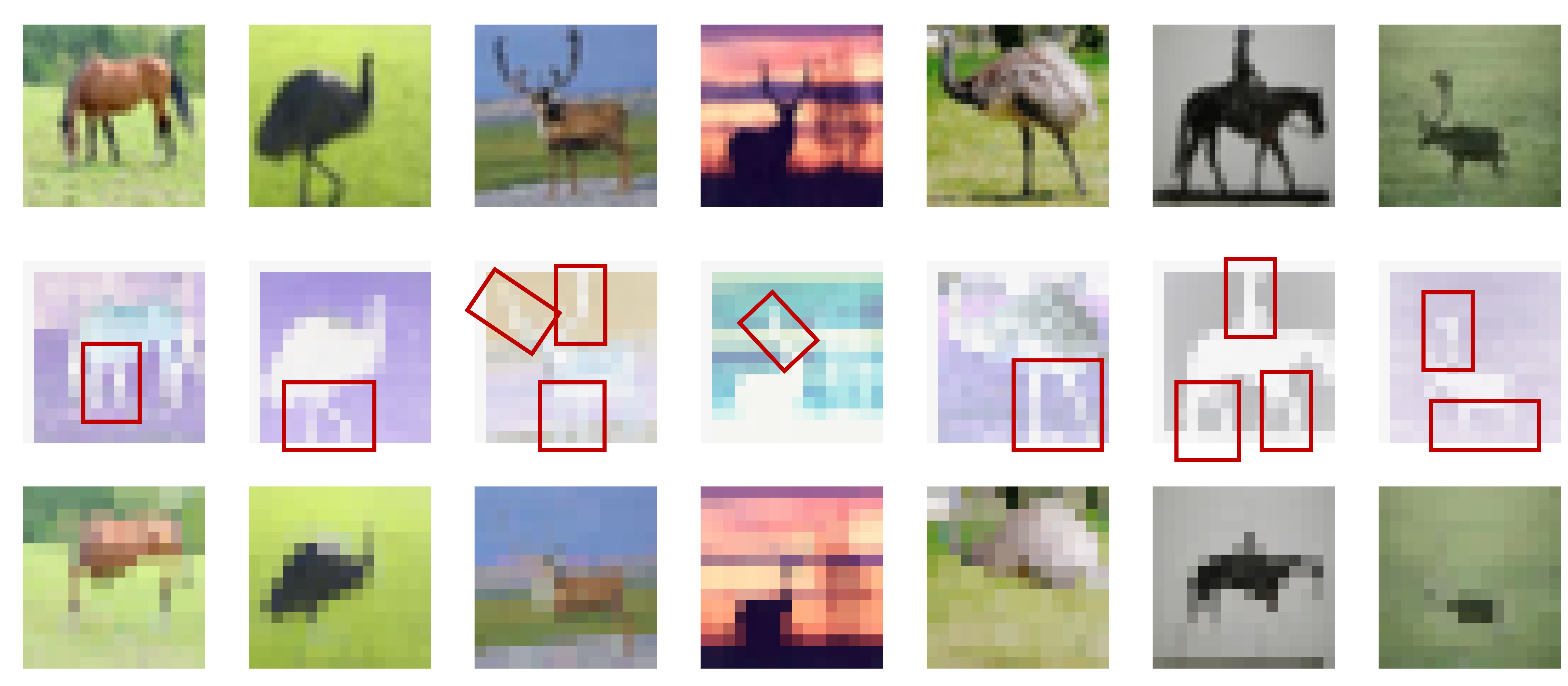
Figure 1: Visualization of images after different downsampling methods on CIFAR-10. Top: Original images. Middle: Quantum Downsampling (Ours). Bottom: Max pooling. Both are with kernel size to be $3\times 3$, stride to be $2$, and padding to be $1$. More details are provided in the supplementary material as the space limitation.

1 Introduction

Max Pooling is a subsampling technique commonly used in deep learning, especially in convolutional neural networks (CNNs) LeCun et al. (1989); Lecun et al. (1998). It is often used to reduce the spatial size of data and computational complexity and increase the receptive field of neurons in subsequent layers. Although the maximum value in max pooling can carry salient features, the features that are not selected during the pooling process are discarded, resulting in a loss of information Boureau et al. (2010).

Recently, there has been a growing interest in applying quantum computing in computer vision Birdal et al. (2021); Golyanik and Theobalt (2020); Meli et al. (2022); Cong et al. (2019); Zhang et al. (2023); Farina et al. (2023); Silver et al. (2023). These quantum algorithms not only hold the promise of tackling intractable problems more effectively but also unveil new patterns and insights within large datasets that are currently beyond the reach of classical computational methods. The quantum-inspired and quantum-enabled algorithms have been adopted in various tasks, including machine learning (ML) Cerezo et al. (2022); Caro et al. (2022), natural language processing (NLP) Li et al. (2019), computer vision (CV) Tang et al. (2022); Golyanik and Theobalt (2020); Meli et al. (2022); Benkner et al. (2021), and multimodal analysis Gkoumas et al. (2021); Li et al. (2021).

However, in the noisy intermediate scale quantum (NISQ) era McClean et al. (2016); Benedetti et al. (2019); Preskill (2018a), quantum computers cannot perform complex quantum algorithms for practical applications. Qubits and their operations are prone to errors due to quantum decoherence and other quantum noise. High error rates in qubit operations and quantum gate functions pose a major challenge to the accuracy of quantum algorithms. Quantum noise can lead to errors and information loss, which is particularly detrimental for quantum neural networks that require high precision.

The current limitations of quantum computing technology have shifted scientific focus towards hybrid quantum-classical neural network architectures Gyongyosi and Imre (2019); Perdomo-Ortiz et al. (2017); Yang and Sun (2022); Doan et al. (2022); Bravyi et al. (2022); Domingo et al. (2023); Pan et al. (2023); Bhatia et al. (2023). These are viewed as a more pragmatic approach compared to the purely quantum computational frameworks due to the relatively higher noise immunities and the implementability of hybrid quantum neural networks.

Inspired by hybrid quantum architecture, we propose a hybrid quantum downsampling module (HQD), which overcomes the limitations of the classical max pooling method in existing classical deep learning models. HQD module can be applied to any state-of-the-art (SOTA) deep learning model as an alternative to max pooling to explore deeper nonlinear relationships between features, as shown in Fig. 1. We use red circles to highlight the features that are easily overlooked in max pooling. Quantum computing brings us a wonderful new perspective on the world.

Within the existing framework of classical computing, no known algorithm is capable of simulating the behavior of a quantum computer Preskill (2018b). This study unveils the distinctive features observable in the quantum realm by employing quantum variational circuits. Different from the feature maps seen by classical max pooling, the quantum downsampling we propose shows us a completely different computer vision in the quantum field in Fig. 1. This process is fundamentally a downsampling procedure, markedly divergent from that of classical computers, capturing a richer array of details. We believe this will play a milestone role in the development of quantum computer vision in the future.

2 Related Work

In this section, we mainly focus on prior work related to quantum computing, quantum computer vision, and hybrid quantum-classical architecture.

Quantum Computing. Quantum computing has experienced a meteoric rise as a focal point of interdisciplinary research, with significant strides being made in the development of quantum hardware De Leon et al. (2021); Kandala et al. (2017); Wang et al. (2023). Parallel to these hardware advancements, the field of quantum algorithmsZhang et al. (2023); Huang et al. (2023); Domingo et al. (2023) has seen a surge in activity.

Quantum Computer Vision. Quantum computer vision (QCV) is an exciting and evolving field with the potential to revolutionize how machines interpret visual data. Quantum approaches have been identified as catalysts for accelerating data processing capabilities and enhancing the performance of analytical models. Over the past few years, researchers have proposed several quantum-based algorithms aimed at addressing various computer vision tasks such as shape matching Golyanik and Theobalt (2020); Meli et al. (2022); Benkner et al. (2021), object tracking Li and Ghosh (2020); Zaech et al. (2022), point triangulation Doan et al. (2022), motion segmentation Arrigoni et al. (2022) and image classification Zhang et al. (2023), multi-model fitting Farina et al. (2023), image generation Silver et al. (2023), point set registration Meli et al. (2022), permutation synchronization Birdal et al. (2021), and shape-matching Benkner et al. (2021).

Hybrid Quantum-Classical Architecture. Based on the advantages of hybrid quantum-classical architecture Gyongyosi and Imre (2019); Perdomo-Ortiz et al. (2017); Doan et al. (2022), related work has gradually begun to appear in the field of computer vision in recent years Yang and Sun (2022). Bravyi Bravyi et al. (2022) formulated a variation of the Quantum Approximate Optimization Algorithm (QAOA) using qudits which is applicable to non-binary combinatorial optimization. Domingo Domingo et al. (2023) proposed a hybrid quantum-classical three-dimensional convolutional neural network where one or more convolutional layers are replaced by quantum convolutional layers. Pan Pan et al. (2023) introduced an innovative approach to hybrid quantum-classical computing by integrating a novel Hadamard Transform (HT)-based layer into neural networks. Bhatia Bhatia et al. (2023) proposed a new quantum-hybrid method for solving the problem of multiple matching of non-rigidly deformed 3D shapes.

3 Methodology

3.1 Quantum Downsampling

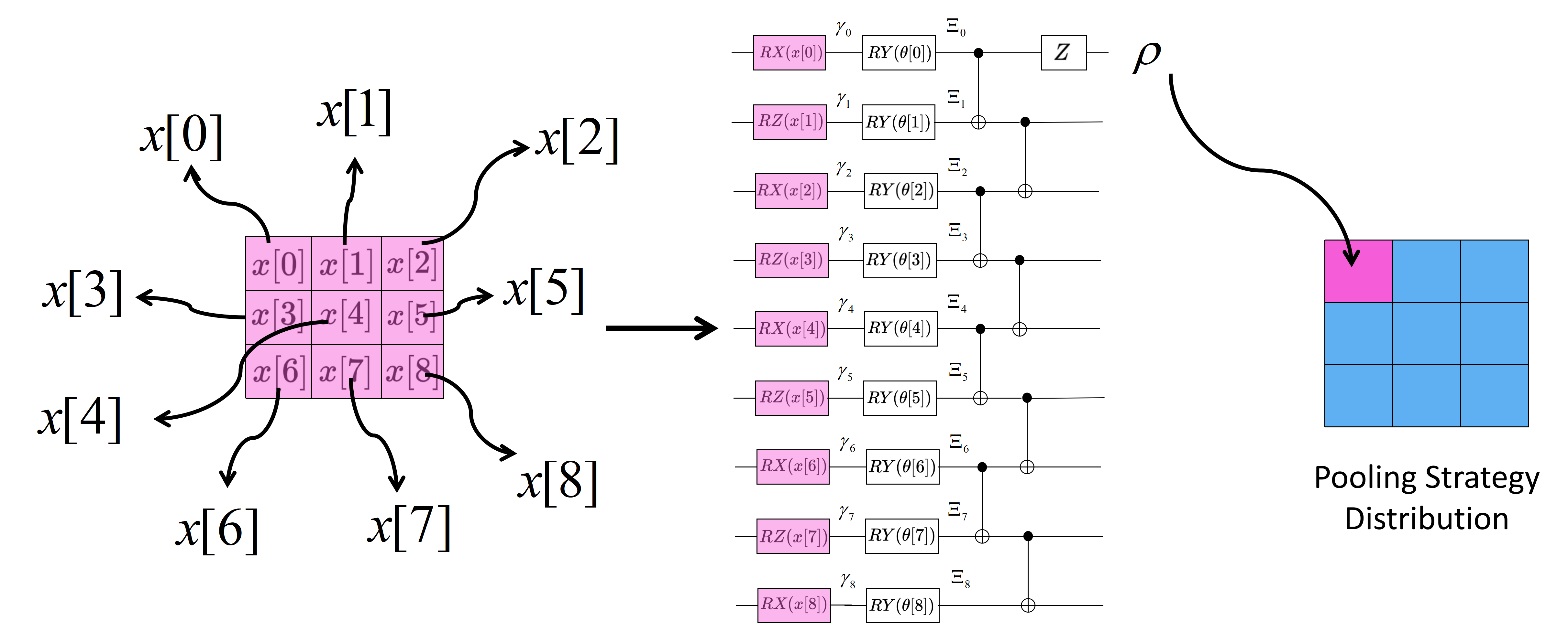
Figure 2: Structure of $3\times 3$ quantum downsampling: it shows the $3\times 3$ pooling window, extracts $9$ eigenvalues, and inputs them into the quantum variational circuit to obtain an output. Pink color indicates the use of quantum downsampling. Pink color in the quantum variational circuit $x[0]-x[8]$ is the value from the input image, and $\theta$ is the parameters to be optimized and $\gamma$, $\Xi$ are values in quantum variational circuit. Blue color indicates the use of classical max pooling. The pooling strategy distribution is determined by $\ell$. The $2\times 2$ quantum downsampling structure is placed in Appendix Fig. 5.

This section presents the framework of the quantum downsampling method with kernel size to be $2\times 2$ and $3\times 3$ with $4$ qubits and $9$ qubits, respectively. Since the internal max-pooling of most SOTA models uses a $3\times 3$ kernel size, only the $3\times 3$ HQD module is discussed in this section, and the relevant parts of $2\times 2$ are placed in supplementary materials. We proposed the forward propagation process of quantum variational circuits throughout the network as well as the gradient descent process.

In Fig. 2, the design of the HQD quantum variational circuit consists of $RX$, $RY$, $RZ$ gates, and CNOT gates, among which Pauli-Z is used to measure the final output. For $RX$ and $RZ$, the rotation amplitude is determined by the value of the input feature map $x$, but for RY, the rotation amplitude is determined by an optimizable parameter $\theta$.

As for the quantum variational circuit of HQD, part of it is an alternating design of $RX$ and $RZ$. The $RX$ and $RZ$ gates are rotation operations of the qubit state on the Bloch ball, rotating around the x-axis and z-axis shown in Fig. 3, respectively. By using these two rotations alternately, quantum states can be explored in different dimensions, increasing the ability of quantum circuits to cover Bloch spheres. The $RY$ gate provides rotation around the y-axis shown in Fig. 3, further increasing the ability to explore the third dimension. This comprehensive rotation strategy helps generate richer and more diverse quantum states. Rotations in different axes have different sensitivities to different system errors, and using them alternately can help spread the effects of these errors.

By inserting a CNOT gate (used to generate entanglement between two qubits) between quantum gate operations (such as $RX$ and $RZ$ rotation), the entanglement between qubits can be effectively generated and controlled. The design strategy of alternately using $RX$ and $RZ$ structures with $RY$ gates increases the exploration capabilities, expression capabilities, and entanglement generation capabilities of quantum circuits, as well as providing error mitigation and flexibility.

Figure 3: Bloch sphere representation of the quantum state $\left|\rho\right\rangle$ during the quantum downsampling. Rotation logic gates $RX$ gate (Left), $RY$ gate (Middle), and $RZ$ gate (Right) for single qubit.

The introduction of optimizable parameters $\theta$ into quantum circuits, especially the use of these parameters in $RY$ gates, makes the circuit parametric. This means that the output of the circuit can be optimized by adjusting these parameters to minimize a certain loss function or achieve a certain computational goal. The $RY$ gate directly adjusts the probability amplitude of the qubit, affecting its probability of being in the $\left|0\right\rangle$and $\left|1\right\rangle$ states. It is very suitable for controlling the degree of superposition of quantum states and realizing conversion between quantum states.

A unitary operator $U(\cdot)$ for the quantum circuit is defined as

$$U=\exp\left({i\alpha}\right)\left[{I\cos\frac{\theta}{2}-i\left({\vec{\sigma}.\hat{n}}\right)\sin\frac{\theta}{2}}\right]\times\exp\left[{-i\frac{\theta}{2}\left({\vec{\sigma}.\hat{n}}\right)}\right],$$ (1)

where ${\vec{\sigma}.\hat{n}}=\sigma_{x}n_{x}+\sigma_{y}n_{y}+\sigma_{z}n_{z}$. The operator $U(\cdot)$ can readily be obtained in simplified form as illustrated in Eq. (2). The variables $\varpi,\chi,\Lambda$, and $\nu$ are all real numbers.

$$U=\left[\begin{array}[]{cc}e^{i\left(\varpi-\frac{\chi}{2}-\frac{\Lambda}{2}\right)\cos\frac{\nu}{2}}&-e^{i\left(\varpi-\frac{\chi}{2}+\frac{\Lambda}{2}\right)\sin\frac{\nu}{2}}\\ e^{i\left(\varpi+\frac{\chi}{2}-\frac{\Lambda}{2}\right)\sin\frac{\nu}{2}}&e^{i\left(\varpi+\frac{\chi}{2}+\frac{\Lambda}{2}\right)\cos\frac{\nu}{2}}\end{array}\right].$$ (2)

Let $RX(\theta)$ be the rotation operator that rotates the qubit through angle $\theta{\rm(radians)}$ around the $X-$axis. It is defined as

$$RX\left(\theta\right)=\left[{\begin{array}[]{*{20}c}{\cos\frac{\theta}{2}}&{-i\sin\frac{\theta}{2}}\\ {-i\sin\frac{\theta}{2}}&{\cos\frac{\theta}{2}}\\ \end{array}}\right].$$ (3)

Applied to any arbitrary pixel $x[k]$, the rotation operator $RX(x[k])$ yields an output as illustrated in Eq. (4):

$$x[k]\xrightarrow[]{RX(x[k])}\gamma=\cos\frac{\theta}{2}\left(\left|0\right\rangle\langle\left.0\right|+\left|1\right\rangle\langle\left.1\right|\right)x[k]-i\sin\frac{\theta}{2}\left(\left|1\right\rangle\langle\left.0\right|+\left|0\right\rangle\langle\left.1\right|\right)x[k].$$ (4)

The output of $RX(\theta)$ and $RZ(\theta)$ operations are then applied to the quantum gate $RY(\theta)$, defined as

$$RY\left(\theta\right)=\left[{\begin{array}[]{*{20}c}{\cos\frac{\theta}{2}}&{-\sin\frac{\theta}{2}}\\ {\sin\frac{\theta}{2}}&{\cos\frac{\theta}{2}}\\ \end{array}}\right].$$ (5)

The output $\gamma$ is fed to the input of the gate $RY(\theta)$, which yields an output defined as depicted in Eq. (6):

$$\begin{split}&\gamma_{j}\hskip 5.69046pt\xrightarrow[]{RY(\gamma_{j})}\Xi_{j}=\hskip 5.69046pt\cos\frac{\theta}{2}\left({\left|0\right.\rangle\langle\left.0\right|+\left|1\right.\rangle\langle\left.1\right|}\right)\gamma_{j}\\ &+\sin\frac{\theta}{2}\left({\left|1\right.\rangle\langle\left.0\right|-\left|0\right.\rangle\langle\left.1\right|}\right)\gamma_{j};j\in\{0,1,\cdot\cdot\cdot,J\}.\end{split}$$ (6)

As shown in Fig. 2, the $RZ(\cdot)$ is defined as

$$RZ(\theta)=e^{\frac{-i\theta Z}{2}}=\cos\left(\frac{\theta}{2}\right)I-i\sin\left(\frac{\theta}{2}\right).$$ (7)

In Fig. 2, the index $j$ represents the index of the wire in the quantum circuit. $J=3$ for $2\times 2$ quantum downsampling kernel and $J=8$ for $3\times 3$ quantum downsampling kernel. The quantum gate $Z$, as illustrated in Fig. 2 corresponds to the Pauli-Z gate and is represented by

$$Z\left(\Xi\right)=\left[{\begin{array}[]{*{20}c}1&0\\ 0&{-1}\\ \end{array}}\right]\Xi.$$ (8)

The corresponding output $\rho$ can then be evaluated as

$$\rho=\left({\left|0\right.\rangle\langle\left.0\right|-\left|1\right.\rangle\langle\left.1\right|}\right)\otimes\Xi,$$ (9)

where $\otimes$ denotes the tensor product operation. $\Xi$ propagates through the controlled NOT gate. The control not gate, $N_{C}(\cdot)$ is defined as

$$N_{C}\left(\theta\right)=\exp\left({i\frac{\pi}{4}\left({I-Z}\right)\left({I-X}\right)}\right).$$ (10)

It can be easily shown that

$$N_{C}\left(\theta\right)N_{C}^{{\dagger}}\left(\theta\right)=I,$$ (11)

where $I$ represents the identity matrix.

3.2 Quantum Measurement of $|\rho\rangle$ for Quantum Downsampling

Let $\mathcal{O}_{l}$ be the measurement operator acting on the quantum state $|\rho\rangle$. The index $l$ depicts the measurement outcomes that may occur in the process. For the given quantum state $|\rho\rangle$, the probability that result $l$ occurs after the quantum measurement is given by

$${\rm P}_{r}\left(l\right)=\langle\rho{|\mathcal{O}_{l}^{\dagger}\mathcal{O}_{l}\left|{\rho}\right.}\rangle.$$ (12)

The quantum state after the measurement can then readily be estimated as

$$\left|{\rho^{l}\rangle}\right.=\frac{{\mathcal{O}_{l}\left|{\rho}\right.\rangle}}{{\sqrt{\langle\rho{|\mathcal{O}_{l}^{\dagger}\mathcal{O}_{l}\left|{\rho}\right.}\rangle}}}.$$ (13)

Since, by the law of total probability, $\sum\limits_{l}{{\rm P}_{r}\left(l\right)}=\sum\limits_{l}{\langle\rho|{\mathcal{O}_{l}^{\dagger}\mathcal{O}_{l}\left|{\rho}\right.}\rangle=1}$, it can be readily shown that the measurement operators $\{\mathcal{O}_{l}\};\forall l$ satisfy the completeness equation as

$$\sum\limits_{l}{\mathcal{O}_{l}^{\dagger}\mathcal{O}_{l}=I}.$$ (14)

Moreover, for any quantum state $\left|\rho\rangle\right.$, the probability of obtaining result $l$ can then be written as

$$\begin{split}&{\rm P}_{r}\left(l\right)=\sum\limits_{j=1}^{J}{{\rm tr}\left({\mathcal{O}_{l}^{\dagger}\mathcal{O}_{l}\sum\limits_{j=1}^{J}{\left.{{\rm P}_{r}}\right|\rho\rangle\langle\left.{\rho}\right|}}\right)},\\ \end{split}$$ (15)

where ${\rm tr(\cdot)}$ is the trace operator. The quantum state representation during the quantum downsampling process is illustrated in Fig. 3.

$RX$, $RY$ can bring changes in probability amplitude in Eq. (3) and Eq. (5), while $RZ$ only changes in phase in Eq. (7). Using these three operations together allows quantum states to move freely throughout the Bloch sphere or in the Hilbert space. By mixing three different quantum gate operations, more in-depth image nonlinear relationships can be explored, and therefore, the hybrid quantum learning model can perform the classification operation with improved performance.

3.3 Quantum Downsampling Gradient Descent

The learning of the proposed HQD is represented by the pooling gradient, as shown in Eq. (16)

$$\frac{\mathrm{d}\left\langle\mathcal{O}_{l}\right\rangle}{\mathrm{d}{\theta_{i}}}\approx\frac{1}{2}\left[\left\langle\mathcal{O}_{l}\right\rangle\left(\theta_{i}+\pi/2\right)-\left\langle\mathcal{O}_{l}\right\rangle\left(\theta_{i}-\pi/2\right)\right].$$ (16)

During the training of the hybrid quantum model, the updated rule of the quantum downsampling gradient descent can be expressed as

$$\Theta_{t+1}\leftarrow\Theta_{t}-\eta\frac{{d\langle\mathcal{O}_{l}\rangle}}{{d\theta_{i}}},$$ (17)

where $\eta$ represents the learning rate.

To quantify the performance of the hybrid quantum-classical approach, we define the loss function as illustrated in Eq. (18) $\mathcal{L}$:

$$\mathcal{L}=-\frac{1}{N}{\textstyle\sum_{i=1}^{N}}{\textstyle\sum_{c=1}^{C}}y_{ic}\log{\hat{y}_{ic}},$$ (18)

where $N$ is the number of samples, $C$ is the number of classes, $y_{ic}$ is $1$ if the $i_{th}$ sample belongs to class $c$ and $0$ otherwise (one-hot encoding of the labels), and ${\hat{y}_{ic}}$ is the predicted probability (output of softmax in the last layer of the neural network) of the $i_{th}$ sample belonging to class $c$. It is to be noted that $\mathcal{L}$ reflects the sum of products of the expected value and log of the predicted value of all the pixels in the hybrid quantum-classical learning model.

3.4 Whole Process of the HQD Module

$\ell$ determines when to perform classical max pooling and when to perform the quantum downsampling process, as shown in the Algorithm. 1. When it comes to quantum downsampling, the whole process is as follows:

Extraction of Values. The value of each of the nine pixels within the $3\times 3$ pooling window is extracted. The initial classical pixels $x[\cdot]$ are first processed through the quantum unitary operator $U(\cdot)$, and subsequently through the quantum gates $RX$, $RZ$ and $RY(\cdot)$ and Pauli-Z, respectively.

Application to the Quantum Variational Circuit. The extracted values are then applied to a quantum variational circuit. These circuits are characterized by a set of parameters that can be tuned or optimized during the process. The input from the pooling window (the extracted pixel values) is used to set or adjust these parameters.

Obtaining Measurement Output. After the quantum variational circuit processes the input data (the qubits corresponding to the $3\times 3$ pooling window), a measurement operator $\mathcal{O}_{l}$ is operated on the quantum state $\rho$ of the system, which yields the output with probability ${\rm P}_{r}(l)$. This measurement yields an output $\left|{\rho^{l}\rangle}\right.$, which is a processed value or set of values derived from the original $3\times 3$ pixel data. In quantum computing, measurements typically collapse the superposed states of qubits into definite quantum states $|\rho\rangle$, which can then be interpreted or further processed.

4 Quantum Noise

To assess and enhance the resilience of quantum neural networks amidst disturbances, we introduced quantum errors in our experiments.

Amplitude Damping. The amplitude damping channel models the process where energy is lost to the surroundings, exemplified by a qubit transitioning from the excited state $\left|1\right\rangle$ to the ground state $\left|0\right\rangle$. This channel is depicted for individual qubits as

$$\mathcal{C}\left(\rho\right)=E_{0}\rho E_{0}^{\dagger}+E_{1}\rho E_{1}^{\dagger},$$ (19)

where $E_{0}=\begin{pmatrix}1&0\\ 0&\sqrt{1-\psi}\end{pmatrix}$ and $E_{1}=\begin{pmatrix}0&\sqrt{\psi}\\ 0&0\end{pmatrix}$. In addition, $\psi$ is the amplitude damping probability.

Phase Flip Noise. Given a phase flipping probability $\psi$, this type of noise operates by applying a Pauli $Z$ gate to the quantum state. This action flips the phase of the state $\left|1\right\rangle$ by introducing a negative sign, while the state $\left|0\right\rangle$ remains unaffected. It can be represented as

$$\mathcal{N}(\rho)=(1-\psi)\rho+\psi Z\rho Z.$$ (20)

Bit Flip Noise. Bit flip noise transforms the state of a qubit from $\left|0\right\rangle$ to $\left|1\right\rangle$ or from $\left|1\right\rangle$ to $\left|0\right\rangle$ with a probability $\psi$, mirroring the effect of a classical bit flip error. Utilizing the Pauli-X operation, the updated state of $\rho$ is expressed as follows:

$$\mathcal{N}(\rho)=(1-\psi)\rho+\psi X\rho X.$$ (21)

Depolarizing Noise. This noise models the information loss that occurs when a qubit interacts with its environment, potentially rendering the qubit’s state entirely random with a given probability. Such interactions lead to a decline in the integrity of quantum information. The state of the qubit under depolarizing noise is shown in Nielsen and Chuang (2010) as

$$\mathcal{N}\left(\rho\right)=\frac{\psi I}{2}+\left(1-\psi\right)\rho.$$ (22)

For the operator-sum representation, we can expand the mixed state $I/2$ as

$$\frac{I}{2}=\frac{\rho+X\rho X+Y\rho Y+Z\rho Z}{4},$$ (23)

and replace the $I/2$ in Eq. 22 and it can be derived as

$$\mathcal{N}\left(\rho\right)=\left(1-\frac{3}{4}\psi\right)\rho+\frac{X\rho X+Y\rho Y+Z\rho Z}{4}\psi.$$ (24)

With the probability $\psi$, we can make Eq. 24 as

$$\mathcal{N}\left(\rho\right)=\left(1-\psi\right)\rho+\frac{\psi}{4}(X\rho X+Y\rho Y+Z\rho Z).$$ (25)

Depolarizing noise causes the state of a qubit to transition to a completely mixed state with probability $\psi$, while it remains unchanged with a of $1-\psi$.

5 Experimental Evaluation

5.1 Hyperparameter Selection and Computing Resources

The CIFAR-10 dataset is normalized with the mean (0.4914, 0.4822, 0.4465) and the standard deviation (0.247, 0.243, 0.261). We adopt the stochastic gradient descent (SGD) Robbins (1951) optimizer with momentum to be $0.9$ and weight decay to be $5e^{-4}$. The initial learning rate $\eta$ is set to $1e^{-3}$ and decreased by a factor of $10$ every $200$ epochs. The batch size is $128$, and the training epochs are $500$. We set up the simulation of a quantum variational circuit based on Pennylaneet al. (2018). All the experiments are performed on an NVIDIA $3060$ GPU and $48$ GB RAM and an NVIDIA $4080$ GPU and $64$ GB RAM. The CIFAR-100 dataset is normalized with the mean (0.4914, 0.4822, 0.4465) and the standard deviation (0.247, 0.243, 0.261). We adopt the stochastic gradient descent (SGD) Robbins (1951) optimizer with momentum to be $0.9$ and weight decay to be $3e^{-4}$. The initial learning rate $\eta$ is set to $1e^{-2}$ and decreased by a factor of $5$ every $30$ epochs. The batch size is $128$, and the training epochs are $100$. For the experiment under quantum noise, including amplitude damping noise, phase flip noise, bit flip noise, and depolarizing noise, we ran the experiment $10$ times, and the noise factor $\psi$ is set to be $0.5$. More details of the structure of HQD models are in Appendix Section E to Section I. In addition, the line plots and scatter plots of Table. 2, Table. 3 and Table. 4 are provided in Appendix Fig.6 and Fig.7.

5.2 Experimental Results

5.2.1 CIFAR-10.

From Table 1, it is evident that HQD has notably enhanced the performance of classical models, albeit with varying degrees of improvement across different architectures. Notably, ResNet-18 benefits the most from the HQD module, witnessing an improvement rate of $3.8\%$. However, when $\ell=300$, the enhancement becomes negligible. On the other hand, the least improvement is observed in the Xception and Attention-56 models.

Table 1: Experimental Results (Accuracy $(\%)$) on CIFAR-10 dataset.

Backbone	Original	HQD ($\ell=100$)	HQD ($\ell=300$)	Parameters (M)
ResNet-18 He et al. (2016)	$75.50$	$\textbf{78.36}\pm\textbf{0.32}$	$75.81\pm 0.29$	$11.22^{\dagger}$
Attention-56 Wang et al. (2017)	$71.86$	$72.54\pm 0.19$	$\textbf{72.74}\pm\textbf{0.24}$	$55.70^{\dagger}$
Xception Chollet (2016)	$79.29$	$79.77\pm 0.08$	$\textbf{79.87}\pm\textbf{0.06}$	$20.83^{\dagger}$
SE-ResNet-18 Hu et al. (2017)	$76.36$	$\textbf{78.19}\pm\textbf{0.15}$	$76.68\pm 0.11$	$11.20^{\dagger}$
SqueezeNet Iandola et al. (2016)	$78.86$	$\textbf{80.01}\pm\textbf{0.37}$	$79.01\pm 0.28$	$0.73^{\dagger}$
NASNet-A Zoph et al. (2017)	$81.15$	$83.33\pm 0.25$	$\textbf{83.41}\pm\textbf{0.29}$	$5.13^{\dagger}$
$\dagger$ indicates $9$ more parameters in the HQD variational circuit.
Bold areas mean better performance under the same model between the two $\ell$s.

5.2.2 CIFAR-100.

This section delves deeper into our analysis by employing the more complex CIFAR-100 dataset. CIFAR-100 contains $60,000$ $32\times 32$ pixel color images, CIFAR-100 contains $100$ categories, and each category contains $600$ images. We tested four $\ell$ values $(50,100,500,1000)$ to explore the impact of different participation levels of the HQD module on the classic model. Based on the experimental results shown in Table. 2, Table. 3 and Table. 4, the best top-1 error and top-5 error of most models are concentrated in the HQD models with $\ell=100$. It is observed that both extremes of $\ell$—too small, indicating minimal HQD participation in the pooling process, and too large, denoting extensive HQD involvement—are detrimental to HQD’s effectiveness in enhancing the performance of classical models. Max pooling simplifies the feature map by extracting the maximum value within a local area, which is effective but may lead to information loss. HQD seeks to minimize information loss with intricate processing. However, overdependence on HQD can overly complicate the model’s extracted features, impairing performance. Striking an optimal balance is crucial to ensure effective feature extraction and mitigate overfitting risks.

Table 2: Experimental Results on CIFAR-100 for ResNet-50 and ResNeXt-50.

Method	Top-1 err. ($\%$) $(\downarrow)$	Top-5 err. ($\%$)$(\downarrow)$	Parameters (M) $(\downarrow)$
ResNet-50 He et al. (2016)	$49.88$	$23.79$	$23.71$
HQD ResNet-50 ($\ell=50$)	$50.28\pm 0.21$	$24.53\pm 0.18$	$23.71^{\dagger}$
HQD ResNet-50 ($\ell=100$)	$\pagecolor{red!50}47.89\pm 0.24$	$\pagecolor{red!50}22.37\pm 0.22$	$23.71^{\dagger}$
HQD ResNet-50 ($\ell=500$)	$51.59\pm 0.19$	$25.19\pm 0.18$	$23.71^{\dagger}$
HQD ResNet-50 ($\ell=1000$)	$\pagecolor{yellow!40}49.55\pm 0.17$	$\pagecolor{yellow!40}23.26\pm 0.21$	$23.71^{\dagger}$
ResNeXt-50 Xie et al. (2016)	$53.18$	$26.37$	$14.79$
HQD ResNeXt-50 ($\ell=50$)	$\pagecolor{yellow!40}52.93\pm 0.43$	$26.91\pm 0.29$	$14.79^{\dagger}$
HQD ResNeXt-50 ($\ell=100$)	$\pagecolor{red!50}52.81\pm 0.27$	$\pagecolor{red!50}26.00\pm 0.40$	$14.79^{\dagger}$
HQD ResNeXt-50 ($\ell=500$)	$54.00\pm 0.31$	$27.19\pm 0.38$	$14.79^{\dagger}$
HQD ResNeXt-50 ($\ell=1000$)	$54.02\pm 0.31$	$26.82\pm 0.35$	$14.79^{\dagger}$
$\dagger$ indicates $9$ more parameters in the HQD variational circuit.
We color each cell as best and second best and best means better than the classical approach.

Furthermore, it’s important to highlight that while HQD Xception shows improvement on the CIFAR-10 dataset, its performance on CIFAR-100 sees negligible enhancement from the HQD module, regardless of the $\ell$ value except $\ell=100$ for top-5 error in Table. 4. CIFAR-100 has more categories and higher intra-category variability than CIFAR-10, which requires the model to be able to extract more complex and detailed features. Although the Xception model performs well in extracting and managing high-level features, efficiently utilizing parameters through depth-separable convolution, and conducting fine spatial and channel analysis of features, the effect of HQD may be offset by the complexity of the task itself. Conversely, it is observed that Xception exhibited the lowest top-1 and top-5 errors across all tested models, yet its performance remained unaffected by HQD integration. A potential reason is that the model is trying to adapt to more complex data structures and category subdivisions, and generalization capabilities are sacrificed by overreliance on specific pooling strategies. In this case, the model may have learned too specific feature expressions on the training set, and these feature expressions may not be able to generalize to the test set effectively. A possible solution is to carry out more mixing ratios $(\ell)$ of quantum downsampling and maximum pooling to adapt to the high complexity of CIFAR-100 for the Xception model.

Table 3: Experimental Results on CIFAR-100 for Attention-56 and SE-ResNet-50.

Method	Top-1 err. ($\%$) $(\downarrow)$	Top-5 err. ($\%$)$(\downarrow)$	Parameters (M) $(\downarrow)$
Attention-56 Wang et al. (2017)	$56.37$	$30.47$	$55.70$
HQD Attention-56 ($\ell=50$)	$57.83\pm 0.17$	$31.26\pm 0.15$	$55.70^{\dagger}$
HQD Attention-56 ($\ell=100$)	$\pagecolor{red!50}55.69\pm 0.09$	$\pagecolor{red!50}29.67\pm 0.12$	$55.70^{\dagger}$
HQD Attention-56 ($\ell=500$)	$56.58\pm 0.13$	$\pagecolor{yellow!40}30.28\pm 0.15$	$55.70^{\dagger}$
HQD Attention-56 ($\ell=1000$)	$57.66\pm 0.11$	$31.25\pm 0.09$	$55.70^{\dagger}$
SE-ResNet-50 Hu et al. (2017)	$48.06$	$21.45$	$28.78$
HQD SE-ResNet-50 ($\ell=50$)	$47.64\pm 0.07$	$21.47\pm 0.17$	$28.78^{\dagger}$
HQD SE-ResNet-50 ($\ell=100$)	$\pagecolor{orange!40}47.48\pm 0.08$	$\pagecolor{red!50}20.79\pm 0.06$	$28.78^{\dagger}$
HQD SE-ResNet-50 ($\ell=500$)	$\pagecolor{red!50}47.41\pm 0.13$	$\pagecolor{yellow!40}21.27\pm 0.09$	$28.78^{\dagger}$
HQD SE-ResNet-50 ($\ell=1000$)	$\pagecolor{yellow!40}47.47\pm 0.15$	$\pagecolor{orange!40}21.38\pm 0.14$	$28.78^{\dagger}$
$\dagger$ indicates $9$ more parameters in the HQD variational circuit, and best, second best and third best.

Table 4: Experimental Results on CIFAR-100 for Xception and SqueezeNet.

Method	Top-1 err. ($\%$) $(\downarrow)$	Top-5 err. ($\%$)$(\downarrow)$	Parameters (M) $(\downarrow)$
Xception Chollet (2016)	$41.53$	$17.01$	$21.01$
HQD Xception ($\ell=50$)	$42.43\pm 0.09$	$17.93\pm 0.13$	$21.01^{\dagger}$
HQD Xception ($\ell=100$)	$41.69\pm 0.03$	$\pagecolor{red!50}16.97\pm 0.15$	$21.01^{\dagger}$
HQD Xception ($\ell=500$)	$42.19\pm 0.08$	$17.61\pm 0.11$	$21.01^{\dagger}$
HQD Xception ($\ell=1000$)	$42.47\pm 0.12$	$17.22\pm 0.16$	$21.01^{\dagger}$
SqueezeNet Iandola et al. (2016)	$47.27$	$20.45$	$0.78$
HQD SqueezeNet ($\ell=50$)	$\pagecolor{red!50}44.75\pm 0.29$	$\pagecolor{yellow!40}18.69\pm 0.21$	$0.78^{\dagger}$
HQD SqueezeNet ($\ell=100$)	$\pagecolor{yellow!40}45.71\pm 0.23$	$\pagecolor{red!50}18.55\pm 0.27$	$0.78^{\dagger}$
HQD SqueezeNet ($\ell=500$)	$\pagecolor{orange!40}45.99\pm 0.30$	$\pagecolor{orange!40}19.30\pm 0.33$	$0.78^{\dagger}$
HQD SqueezeNet ($\ell=1000$)	$46.02\pm 0.36$	$19.46\pm 0.29$	$0.78^{\dagger}$
$\dagger$ indicates $9$ more parameters in the HQD variational circuit, and best, second best and third best.

Additionally, it was noted that the proposed HQD module exhibited resilience to noise across various experiments, with test results varying within a narrow margin of $\pm 0.4$. One explanation for this is that the HQD model treats quantum noise as part of the deep neural network and adapts to these noises during training. Through gradient descent and optimization one at a time, the parameters of the deep neural network and the parameters in the variational quantum circuit in the HQD module are optimized in this process. This experimental result also proves the robustness of our proposed HQD module.

6 Conclusion

In this study, we proposed an advanced hybrid quantum-classical paradigm, the HQD module, which was predicated upon an innovative mixed pooling methodology. Our pioneering experiments provide empirical evidence that the HQD module can yield a discernible quantum advantage in addressing traditional challenges in computer vision tasks with noise-resilient capabilities. During downsampling, quantum computing can capture more nonlinear features while retaining as much detail as possible. It is worth mentioning that the HQD module can be seamlessly integrated into any SOTA deep learning model. Meanwhile, this novel strategy has the potential to catalyze the development of superior algorithms for a spectrum of applications in computer vision and beyond. We envision that the HQD module will play a vital and meaningful role in image segmentation and edge detection tasks and pave a crucial pathway for the advancement of quantum artificial intelligence (QAI).

Appendix

Algorithm 1 HQD Module

Input: Kernel size: $K$, Padding: $p$, Stride: $s$, training $epoch$
Input: Width and height of the pooling window: $a\times b$, $a$ and $b$ are the pixel index in kernel window $(K-1)\times(K-1)$, hybrid parameter: $\ell$
Initialize: Quantum state: $\rho=|0\rangle$

1:  for $i=1$ to $epoch$ do

2:     for $l_{0}=1$ to $\ell$ do

3:        if $l_{0}\leq\ell-1$ then

4:           Max pooling:

5:           Evaluate: $H_{out}$ and $W_{out}$

6:           Compute: $\tilde{I_{M}}(i,j)=$ $\max_{a=0}^{K-1}\max_{b=0}^{K-1}I(s\cdot i+a-p,s\cdot j+b-p)$

7:        end if

8:        Quantum Downsampling:

9:        Evaluate: ${\rm P}_{r}\left(l\right)=\langle\rho{|\mathcal{O}_{l}^{\dagger}\mathcal{O}_{l}\left|{\rho}\right.}\rangle$

10:     end for

11:  end for

12:  return  Feature map $\tilde{I_{M}}:H_{out}\times W_{out}$.

Appendix A Limitations

Parameters. Due to the quantum variational circuits, there are $9$ more parameters to be optimized in training compared to the classical max pooling method in the various deep learning architectures, which means model training and inference will take longer. However, in Fig. 4, we can see that the introduction of $9$ additional parameters does not significantly increase the computational complexity in the training process. However, increasing parameters means the model requires more memory, which is particularly problematic on resource-constrained devices. Although the additional parameters of quantum downsampling introduce some challenges, better computing resources can minimize the impact of these limitations while improving model performance.

Quantum Hardware. Considering the $3\times 3$ pooling operation, it is noteworthy that merely $9$ qubits are requisite for a quantum computer to fulfill the entire procedure. However, the limitation is twofold: firstly, the current state of quantum hardware, characterized by its qubit fidelity and coherence time, poses challenges to the stability and reliability of executing operations over even a modest number of qubits De Leon et al. [2021]. Secondly, the integration of quantum processes into classical deep learning workflows requires quantum-classical interface mechanisms that can maintain the integrity of the computational process. These considerations underscore the necessity for advancements in quantum hardware and algorithmic strategies, particularly in the context of tasks like pooling operations that are ubiquitous in deep learning architectures.

Quantum Noise. Although quantum noise simulation experiments can provide insights into the theoretical resistance of algorithms to noise, these simulations often have significant gaps with reality. Furthermore, quantum computers also face the challenge of quantum state preparation and readout when processing such large-scale datasets. Likewise, readout errors during the quantum measurement process may also seriously affect the accuracy of the classification results Preskill [2018b]. Current quantum technologies are still limited in precise control and measurement, which is particularly problematic when processing large amounts of data. While simulation experiments provide important insights into how quantum algorithms perform in the face of noise, applying these algorithms to actual quantum hardware and processing large-scale datasets requires a lot of effort.

Appendix B CIFAR-10 dataset

Figure 4: Accuracy versus parameters (left) and accuracy versus different models (right) on CIFAR-10 dataset. Red circles indicate the classical results, and the black shapes stand for our proposed models.

By correlating the data on the number of parameters depicted in Fig. 4 with the more illustrative trend line chart, it becomes apparent that an increase in model parameters theoretically enhances the model’s representational capacity. However, this augmentation simultaneously elevates the likelihood of overfitting. For high-parameter models, the incremental benefits from the HQD module may be limited. These models already capture extensive feature information, making the performance gains from further optimizations less significant compared to models with fewer parameters. Conversely, varying $\ell$ values impact models differently. A higher $\ell$ value indicates reduced involvement of the HQD module.

Appendix C The $2\times 2$ HQD Module and Application

Figure 5: Structure of $2\times 2$ quantum downsampling: it shows the $2\times 2$ pooling window, extracts $4$ eigenvalues, and puts them into the quantum variational circuit to obtain an output. Pink color indicates the use of quantum downsampling. Pink color in the quantum variational circuit $x[0]-x[3]$ are the value from the input image, and $\theta$ is the parameters to be optimized. Blue color indicates the use of classical max pooling. The pooling strategy distribution is determined by $\ell$.

In Fig. 5, the quantum variational circuit for downsampling with a $2\times 2$ kernel is presented. A design similar to the $3\times 3$ quantum variational circuit connects the $RX$ gate to the $RY$ gate and the $RZ$ gate to the $RY$ gate. Then, the CNOT gate is used to create entanglement between them, and finally, the Pauli-Z gate is used to measure the result. Due to the space limitation, we implement the $2\times 2$ quantum downsampling module in the VGG structure in the following section.

Table 5: Experimental Results on CIFAR-100 for VGG-13, VGG-16 and VGG -19.

Method	Top-1 err. ($\%$) $(\downarrow)$	Top-5 err. ($\%$)$(\downarrow)$	Parameters (M) $(\downarrow)$
VGG-13 Simonyan and Zisserman [2014]	$40.86$	$16.31$	$28.15$
HQD VGG-13 ($\ell=50$)	$41.64\pm 0.12$	$17.54\pm 0.13$	$28.15^{\ddagger}$
HQD VGG-13 ($\ell=100$)	$41.27\pm 0.35$	$16.45\pm 0.29$	$28.15^{\ddagger}$
HQD VGG-13 ($\ell=200$)	$41.01\pm 0.45$	$16.43\pm 0.01$	$28.15^{\ddagger}$
HQD VGG-13 ($\ell=300$)	$40.71\pm 0.22$	$16.07\pm 0.18$	$28.15^{\ddagger}$
HQD VGG-13 ($\ell=400$)	$41.13\pm 0.24$	$16.01\pm 0.11$	$28.15^{\ddagger}$
HQD VGG-13 ($\ell=500$)	$41.24\pm 0.31$	$16.36\pm 0.22$	$28.15^{\ddagger}$
HQD VGG-13 ($\ell=1000$)	$41.61\pm 0.04$	$16.11\pm 0.09$	$28.15^{\ddagger}$
VGG-16 Simonyan and Zisserman [2014]	$41.25$	$16.36$	$33.65$
HQD VGG-16 ($\ell=50$)	$41.17\pm 0.11$	$17.60\pm 0.02$	$33.65^{\ddagger}$
HQD VGG-16 ($\ell=100$)	$40.94\pm 0.24$	$16.14\pm 0.27$	$33.65^{\ddagger}$
HQD VGG-16 ($\ell=200$)	$40.84\pm 0.21$	$16.09\pm 0.03$	$33.65^{\ddagger}$
HQD VGG-16 ($\ell=300$)	$40.50\pm 0.33$	$15.92\pm 0.32$	$33.65^{\ddagger}$
HQD VGG-16 ($\ell=400$)	$41.12\pm 0.23$	$16.52\pm 0.19$	$33.65^{\ddagger}$
HQD VGG-16 ($\ell=500$)	$40.60\pm 0.17$	$16.28\pm 0.22$	$33.65^{\ddagger}$
HQD VGG-16 ($\ell=1000$)	$40.67\pm 0.15$	$16.24\pm 0.18$	$33.65^{\ddagger}$
VGG-19 Simonyan and Zisserman [2014]	$42.36$	$18.33$	$38.96$
HQD VGG-19 ($\ell=50$)	$41.40\pm 0.12$	$17.76\pm 0.07$	$38.96^{\ddagger}$
HQD VGG-19 ($\ell=100$)	$41.57\pm 0.26$	$17.10\pm 0.65$	$38.96^{\ddagger}$
HQD VGG-19 ($\ell=200$)	$41.37\pm 0.19$	$17.55\pm 0.19$	$38.96^{\ddagger}$
HQD VGG-19 ($\ell=300$)	$41.48\pm 0.46$	$17.35\pm 0.03$	$38.96^{\ddagger}$
HQD VGG-19 ($\ell=400$)	$41.53\pm 0.31$	$17.74\pm 0.27$	$38.96^{\ddagger}$
HQD VGG-19 ($\ell=500$)	$41.81\pm 0.25$	$17.44\pm 0.27$	$38.96^{\ddagger}$
HQD VGG-19 ($\ell=1000$)	$41.85\pm 0.14$	$17.20\pm 0.11$	$38.96^{\ddagger}$
Best means better than the classical approach.
We color each cell as best, second best, third best and fourth best.
$\ddagger$ indicates $4$ more parameters in the HQD variational circuit for kernel size $2\times 2$.

Table. 5 illustrates that the HQD module yields the most significant enhancement in performance for the VGG-19 architecture, followed by VGG-16, while the improvement observed for VGG-13 is minimal. Notably, within the context of Top-1 error metrics, only a singular configuration manages ($\ell=300$) to improve performance. One possible reason is that the VGG-19 and VGG-16 models have more convolutional layers and parameters than VGG-13 as shown in Fig. 8, which means they are able to benefit from more complex feature extraction and finer-grained feature representation. The HQD module can capture and deliver important feature information more efficiently through its design, which may be more evident in deeper and more complex networks. At the same time, the HQD module is designed to capture and retain important feature information while reducing information loss. In deeper networks, the optimization of information transfer and feature representation may be more critical, so the HQD module improves VGG-19 and VGG-16 more significantly.

From Table. 4, we can also see that classical VGG-13 has the best performance among the classic models. This is because deeper models such as VGG-19 and VGG-16 are more likely to overfit in this case. The HQD module provides an effective form of regularization for these models by improving feature selection and transfer, thereby mitigating overfitting problems while maintaining model capacity. Overfitting is not a major problem for shallower models like VGG-13, so the HQD module’s improvement is not so obvious.

Appendix D Plots of Table. 2, Table. 3 and Table. 4 in the Main Paper

Figure 6: Top-1 error (left) and Top-5 error (right) versus parameters on CIFAR-100 dataset.

Figure 7: Top-1 error (left) and Top-5 error (right) versus different models on CIFAR-100 dataset.

Fig. 6 and 7 reveal varying degrees of performance enhancements across different models attributable to the HQD module. Specifically, the figures highlight an improvement in SqueezeNet’s performance across different $\ell$ values. Regarding the Top-1 error metric, the application of the HQD module, with its varying $\ell$ values, introduces the most significant performance variability in ResNet-50.

Appendix E VGG and HQD VGG Structures

Figure 8: Structure of VGG (Left) and HQD VGG (Right).

In Fig. 8, we showed three kinds of VGG structures, VGG-13, VGG-16, and VGG-19 respectively. For each kind of VGG structure, HQD networks are shown on the right hand. More specifically, the $2\times 2$ max pooling layer in the original VGG structure was replaced by the HQD module with $4$ qubits.

Appendix F SqueezeNet and HQD SqueezeNet Structures

Figure 9: Structure of SqueezeNet (Left) and HQD SqueezeNet (Right).

In Fig. 9, we showed the structure of the classical SqueezeNet model on the left hand Iandola et al. [2016] and the HQD SqueezeNet model on the right hand.

Appendix G Attention Networks and HQD Attention Networks Structures

Table 6: Attention-56 and Attention-92 Wang et al. [2017] Structure

Layer	Output Size	Attention-56	Attention-92
Conv1	$112\times 112$	$7\times 7,64,\text{stride}2$
Max pooling	$56\times 56$	$3\times 3,\text{stride}2$
Residual Unit	$56\times 56$	$\begin{pmatrix}1\times 1&64\\ 3\times 3&64\\ 1\times 1&256\end{pmatrix}\times 1$
Attention Module	$56\times 56$	Attention $\times 1$	Attention $\times 1$
Residual Unit	$28\times 28$	$\begin{pmatrix}1\times 1&128\\ 3\times 3&128\\ 1\times 1&512\end{pmatrix}\times 1$
Attention Module	$28\times 28$	Attention $\times 1$	Attention $\times 2$
Residual Unit	$14\times 14$	$\begin{pmatrix}1\times 1&256\\ 3\times 3&256\\ 1\times 1&1024\end{pmatrix}\times 1$
Attention Module	$14\times 14$	Attention $\times 1$	Attention $\times 3$
Residual Unit	$7\times 7$	$\begin{pmatrix}1\times 1&512\\ 3\times 3&512\\ 1\times 1&2048\end{pmatrix}\times 3$
Average pooling	$1\times 1$	$7\times 7,\text{stride}1$
Softmax	$100$

Table 7: HQD Attention-56 and HQD Attention-92 Structure

Layer	Output Size	Attention-56	Attention-92
Conv1	$112\times 112$	$7\times 7,64,\text{stride}2$
HQD Module	$56\times 56$	$3\times 3,\text{stride}2$
Residual Unit	$56\times 56$	$\begin{pmatrix}1\times 1&64\\ 3\times 3&64\\ 1\times 1&256\end{pmatrix}\times 1$
Attention Module	$56\times 56$	Attention $\times 1$	Attention $\times 1$
Residual Unit	$28\times 28$	$\begin{pmatrix}1\times 1&128\\ 3\times 3&128\\ 1\times 1&512\end{pmatrix}\times 1$
Attention Module	$28\times 28$	Attention $\times 1$	Attention $\times 2$
Residual Unit	$14\times 14$	$\begin{pmatrix}1\times 1&256\\ 3\times 3&256\\ 1\times 1&1024\end{pmatrix}\times 1$
Attention Module	$14\times 14$	Attention $\times 1$	Attention $\times 3$
Residual Unit	$7\times 7$	$\begin{pmatrix}1\times 1&512\\ 3\times 3&512\\ 1\times 1&2048\end{pmatrix}\times 3$
Average pooling	$1\times 1$	$7\times 7,\text{stride}1$
Softmax	$100$

Appendix H SE-ResNet, ResNet, HQD SE-ResNet and HQD ResNet Structures

Table 8: ResNet-18 He et al. [2016] and HQD ResNet-18 Structure

Layer Name	Output Size	ResNet-18	HQD ResNet-18
conv1	$112\times 112\times 64$	$7\times 7$, $64$, stride 2	$7\times 7$, $64$, stride 2
		$3\times 3$ max pool, stride 2	$3\times 3$ HQD module
conv2_x	$56\times 56\times 64$	$\begin{bmatrix}3\times 3,&64\\ 3\times 3,&64\end{bmatrix}\times 2\rule[-17.22217pt]{0.0pt}{34.44434pt}$	$\begin{bmatrix}3\times 3,&64\\ 3\times 3,&64\end{bmatrix}\times 2$
conv3_x	$28\times 28\times 128$	$\begin{bmatrix}3\times 3,&128\\ 3\times 3,&128\end{bmatrix}\times 2\rule[-17.22217pt]{0.0pt}{34.44434pt}$	$\begin{bmatrix}3\times 3,&128\\ 3\times 3,&128\end{bmatrix}\times 2\rule[-12.91663pt]{0.0pt}{25.83325pt}$
conv4_x	$14\times 14\times 256$	$\begin{bmatrix}3\times 3,&256\\ 3\times 3,&256\end{bmatrix}\times 2\rule[-12.91663pt]{0.0pt}{25.83325pt}$	$\begin{bmatrix}3\times 3,&256\\ 3\times 3,&256\end{bmatrix}\times 2\rule[-12.91663pt]{0.0pt}{25.83325pt}$
conv5_x	$7\times 7\times 512$	$\begin{bmatrix}3\times 3,&512\\ 3\times 3,&512\end{bmatrix}\times 2\rule[-17.22217pt]{0.0pt}{25.83325pt}$	$\begin{bmatrix}3\times 3,&512\\ 3\times 3,&512\end{bmatrix}\times 2\rule[-12.91663pt]{0.0pt}{25.83325pt}$
average pool	$1\times 1\times 64$	$7\times 7$ average pool	$7\times 7$ average pool
fully connected	$10$	$512\times 10$	$512\times 10$
softmax	$10$

Table 9: SE-ResNet-18 Hu et al. [2017] and HQD SE-ResNet-18 Structure

Layer Name	Output Size	SE-ResNet-18	HQD SE-ResNet-18
conv1	$112\times 112\times 64$	$7\times 7$, $64$, stride 2	$7\times 7$, $64$, stride 2
		$3\times 3$ max pool, stride 2	$3\times 3$ HQD module
conv2_x	$56\times 56\times 64$	$\begin{bmatrix}3\times 3,&64\\ 3\times 3,&64\\ fc,&[2,64]\end{bmatrix}\times 2\rule[-17.22217pt]{0.0pt}{34.44434pt}$	$\begin{bmatrix}3\times 3,&64\\ 3\times 3,&64\\ fc,&[2,64]\end{bmatrix}\times 2$
conv3_x	$28\times 28\times 128$	$\begin{bmatrix}3\times 3,&128\\ 3\times 3,&128\\ fc,&[4,128]\end{bmatrix}\times 2\rule[-17.22217pt]{0.0pt}{34.44434pt}$	$\begin{bmatrix}3\times 3,&128\\ 3\times 3,&128\\ fc,&[4,128]\end{bmatrix}\times 2\rule[-12.91663pt]{0.0pt}{25.83325pt}$
conv4_x	$14\times 14\times 256$	$\begin{bmatrix}3\times 3,&256\\ 3\times 3,&256\\ fc,&[8,256]\end{bmatrix}\times 2\rule[-12.91663pt]{0.0pt}{25.83325pt}$	$\begin{bmatrix}3\times 3,&256\\ 3\times 3,&256\\ fc,&[8,256]\end{bmatrix}\times 2\rule[-12.91663pt]{0.0pt}{25.83325pt}$
conv5_x	$7\times 7\times 512$	$\begin{bmatrix}3\times 3,&512\\ 3\times 3,&512\\ fc,&[16,512]\end{bmatrix}\times 2\rule[-17.22217pt]{0.0pt}{25.83325pt}$	$\begin{bmatrix}3\times 3,&512\\ 3\times 3,&512\\ fc,&[16,512]\end{bmatrix}\times 2\rule[-12.91663pt]{0.0pt}{25.83325pt}$
average pool	$1\times 1\times 64$	$7\times 7$ average pool	$7\times 7$ average pool
fully connected	$10$	$512\times 10$	$512\times 10$
softmax	$10$

Table 10: ResNet-50 and HQD ResNet-50 Structure

Output size	ResNet-50	HQD ResNet-50
$112\times 112$	conv, $7\times 7$, 64, stride 2
	max pool, $3\times 3$, stride 2	HQD module, $3\times 3$
$56\times 56$	$\begin{bmatrix}\text{conv},&1\times 1,&64\\ \text{conv},&3\times 3,&64\\ \text{conv},&1\times 1,&256\end{bmatrix}\times 3$	$\begin{bmatrix}\text{conv},&1\times 1,&64\\ \text{conv},&3\times 3,&64\\ \text{conv},&1\times 1,&256\end{bmatrix}\times 3$
$28\times 28$	$\begin{bmatrix}\text{conv},&1\times 1,&128\\ \text{conv},&3\times 3,&128\\ \text{conv},&1\times 1,&512\end{bmatrix}\times 4$	$\begin{bmatrix}\text{conv},&1\times 1,&128\\ \text{conv},&3\times 3,&128\\ \text{conv},&1\times 1,&512\end{bmatrix}\times 4$
$14\times 14$	$\begin{bmatrix}\text{conv},&1\times 1,&256\\ \text{conv},&3\times 3,&256\\ \text{conv},&1\times 1,&1024\end{bmatrix}\times 6$	$\begin{bmatrix}\text{conv},&1\times 1,&256\\ \text{conv},&3\times 3,&256\\ \text{conv},&1\times 1,&1024\end{bmatrix}\times 6$
$7\times 7$	$\begin{bmatrix}\text{conv},&1\times 1,&512\\ \text{conv},&3\times 3,&512\\ \text{conv},&1\times 1,&2048\end{bmatrix}\times 3$	$\begin{bmatrix}\text{conv},&1\times 1,&512\\ \text{conv},&3\times 3,&512\\ \text{conv},&1\times 1,&2048\end{bmatrix}\times 3$
$1\times 1$	global average pool, 100-d $fc$, softmax

Table 11: SE-ResNet-50 and HQD SE-ResNet-50 Structure

Output size	SE-ResNet-50	HQD SE-ResNet-50
$112\times 112$	conv, $7\times 7$, 64, stride 2
	max pooling, $3\times 3$, stride 2	HQD module, $3\times 3$
$56\times 56$	$\begin{bmatrix}\text{conv},&1\times 1,&64\\ \text{conv},&3\times 3,&64\\ \text{conv},&1\times 1,&256\\ fc,&[16,256]\rule[-5.16663pt]{0.0pt}{12.91663pt}&\end{bmatrix}\times 3$	$\begin{bmatrix}\text{conv},&1\times 1,&64\\ \text{conv},&3\times 3,&64\\ \text{conv},&1\times 1,&256\\ fc,&[16,256]&\end{bmatrix}\times 3$
$28\times 28$	$\begin{bmatrix}\text{conv},&1\times 1,&128\\ \text{conv},&3\times 3,&128\\ \text{conv},&1\times 1,&512\\ fc,&[32,512]\rule[-5.16663pt]{0.0pt}{12.91663pt}&\end{bmatrix}\times 4$	$\begin{bmatrix}\text{conv},&1\times 1,&128\\ \text{conv},&3\times 3,&128\\ \text{conv},&1\times 1,&512\\ fc,&[32,512]&\end{bmatrix}\times 4$
$14\times 14$	$\begin{bmatrix}\text{conv},&1\times 1,&256\\ \text{conv},&3\times 3,&256\\ \text{conv},&1\times 1,&1024\\ fc,&[64,1024]\rule[-5.16663pt]{0.0pt}{12.91663pt}&\end{bmatrix}\times 6$	$\begin{bmatrix}\text{conv},&1\times 1,&256\\ \text{conv},&3\times 3,&256\\ \text{conv},&1\times 1,&1024\\ fc,&[64,1024]&\end{bmatrix}\times 6$
$7\times 7$	$\begin{bmatrix}\text{conv},&1\times 1,&512\\ \text{conv},&3\times 3,&512\\ \text{conv},&1\times 1,&2048\\ fc,&[128,2048]\rule[-5.16663pt]{0.0pt}{12.91663pt}&\end{bmatrix}\times 3$	$\begin{bmatrix}\text{conv},&1\times 1,&512\\ \text{conv},&3\times 3,&512\\ \text{conv},&1\times 1,&2048\\ fc,&[128,2048]&\end{bmatrix}\times 3$
$1\times 1$	global average pool, 100-d $fc$, softmax

Appendix I ResNeXt and HQD ResNeXt Structures

Table 12: ResNext-50 Xie et al. [2016] and HQD ResNext-50 Structure

Output size	ResNeXt-50 ($32\times 4\text{d}$)	HQD ResNeXt-50 ($32\times 4\text{d}$)
$112\times 112$	conv, $7\times 7$, 64, stride 2
	max pooling, $3\times 3$, stride 2	HQD module, $3\times 3$
$56\times 56$	$\begin{bmatrix}\text{conv},&1\times 1,&128&\\ \text{conv},&3\times 3,&128&,C=32\\ \text{conv},&1\times 1,&256&\\ \end{bmatrix}\times 3$	$\begin{bmatrix}\text{conv},&1\times 1,&128&\\ \text{conv},&3\times 3,&128&,C=32\\ \text{conv},&1\times 1,&256&\rule[-5.16663pt]{0.0pt}{12.91663pt}\\ \end{bmatrix}\times 3$
$28\times 28$	$\begin{bmatrix}\text{conv},&1\times 1,&256&\\ \text{conv},&3\times 3,&256&,C=32\\ \text{conv},&1\times 1,&512&\end{bmatrix}\times 4$	$\begin{bmatrix}\text{conv},&1\times 1,&256&\\ \text{conv},&3\times 3,&256&&,C=32\\ \text{conv},&1\times 1,&512&\rule[-5.16663pt]{0.0pt}{12.91663pt}\end{bmatrix}\times 4$
$14\times 14$	$\begin{bmatrix}\text{conv},&1\times 1,&512\\ \text{conv},&3\times 3,&512&,C=32\\ \ \text{conv},&1\times 1,&1024\rule[-5.16663pt]{0.0pt}{12.91663pt}\end{bmatrix}\times 6$	$\begin{bmatrix}\text{conv},&1\times 1,&512\\ \text{conv},&3\times 3,&512&,C=32\\ \ \text{conv},&1\times 1,&1024\\ \end{bmatrix}\times 6$
$7\times 7$	$\begin{bmatrix}\text{conv},&1\times 1,&1024\\ \text{conv},&3\times 3,&1024&,C=32\\ \ \text{conv},&1\times 1,&2048\rule[-5.16663pt]{0.0pt}{12.91663pt}\\ \end{bmatrix}\times 3$	$\begin{bmatrix}\text{conv},&1\times 1,&1024\\ \text{conv},&3\times 3,&1024&,C=32\\ \ \text{conv},&1\times 1,&2048\\ \end{bmatrix}\times 3$
$1\times 1$	global average pool, 100-d $fc$, softmax

Appendix J Max Pooling and Quantum Downsampling Visualisation

In this section, we present comparative feature maps for max pooling and quantum downsampling, offering an in-depth analysis across various datasets. The illustrations notably utilize red circles to highlight specific details that traditional max pooling overlooks, yet are retained through quantum downsampling.

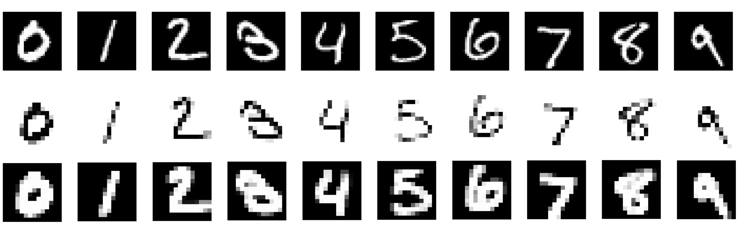
Figure 10: Visualization of images after different downsampling methods on MNIST from $0$ to $10$. Top: Original images. Middle: Quantum Downsampling (Ours). Bottom: Max pooling. Kernel size is to be $3\times 3$, stride is to be $2$, and padding is to be $1$.

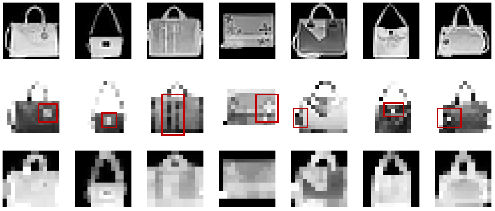
Figure 11: Visualization of images after different downsampling methods on MNIST-Fasion. Top: Original images. Middle: Quantum Downsampling (Ours). Bottom: Max pooling. Both have kernel size to be $3\times 3$, stride to $2$, and padding to $1$.

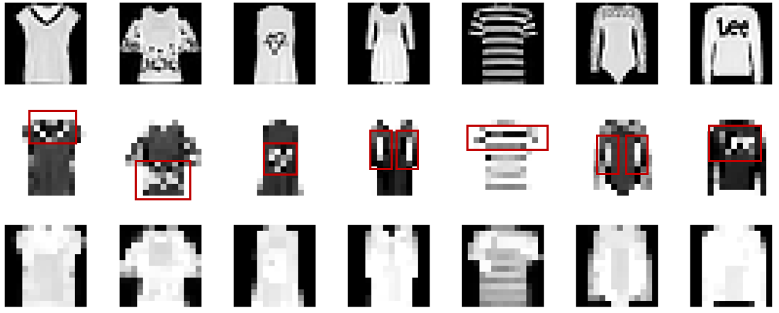
Figure 12: Visualization of images after different downsampling methods on MNIST-Fasion. Top: Original images. Middle: Quantum Downsampling (Ours). Bottom: Max pooling. Both have kernel size to be $3\times 3$, stride to $2$, and padding to $1$.

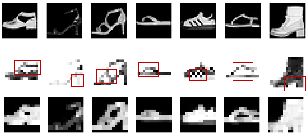
Figure 13: Visualization of images after different downsampling methods on MNIST-Fasion. Top: Original images. Middle: Quantum Downsampling (Ours). Bottom: Max pooling. Kernel size is $3\times 3$, stride is $2$, and padding is $1$.

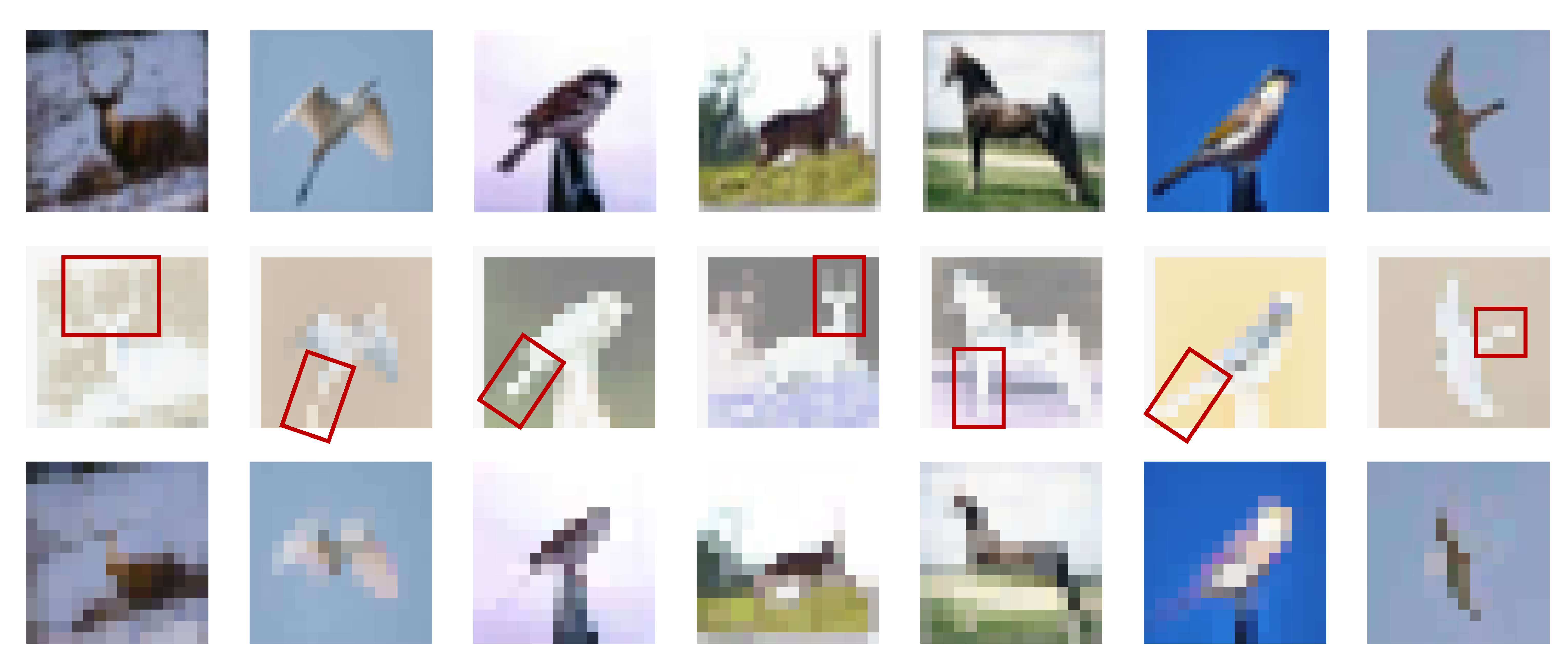
Figure 14: Visualization of images after different downsampling methods on CIFAR-10. Top: Original images. Middle: Quantum Downsampling (Ours). Bottom: Max pooling. Both have kernel size to be $3\times 3$, stride to $2$, and padding to $1$.

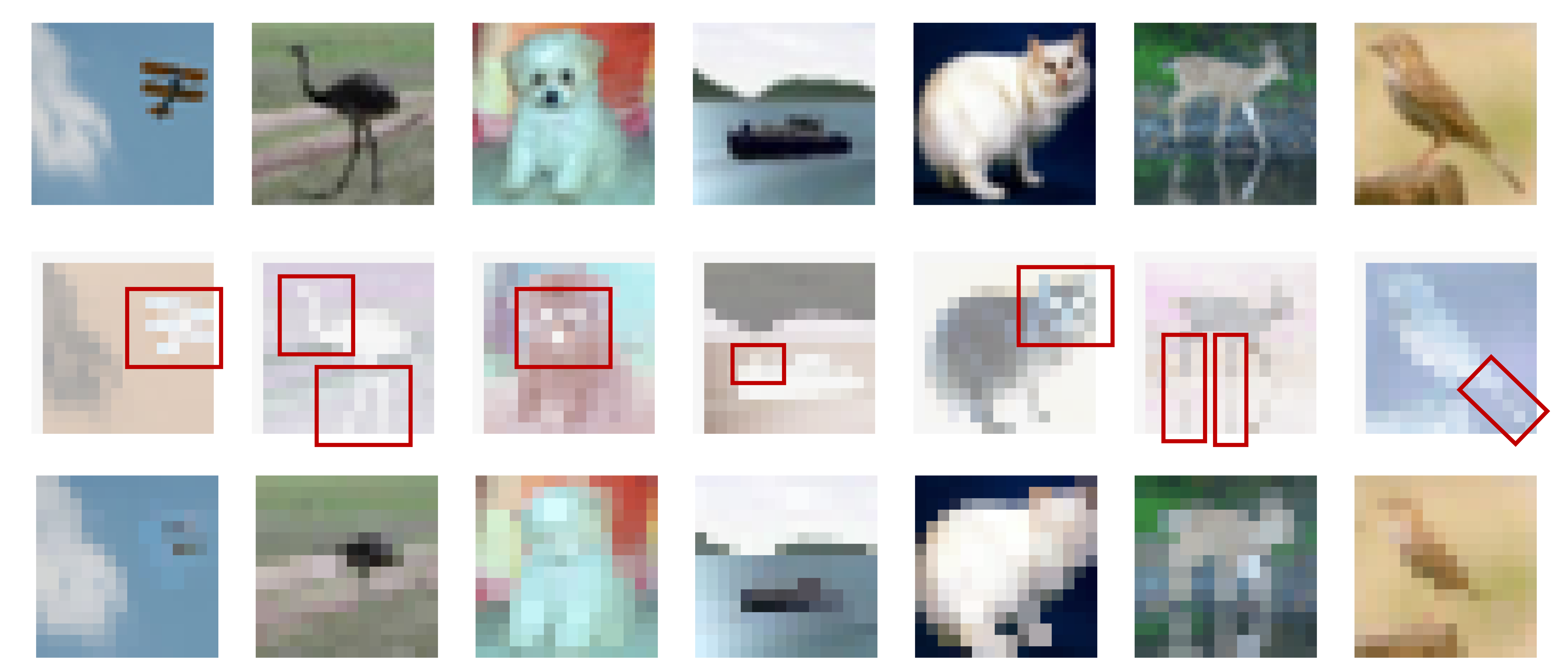
Figure 15: Visualization of images after different downsampling methods on CIFAR-10. Top: Original images. Middle: Quantum Downsampling (Ours). Bottom: Max pooling. Both have kernel size to be $3\times 3$, stride to $2$, and padding to $1$.

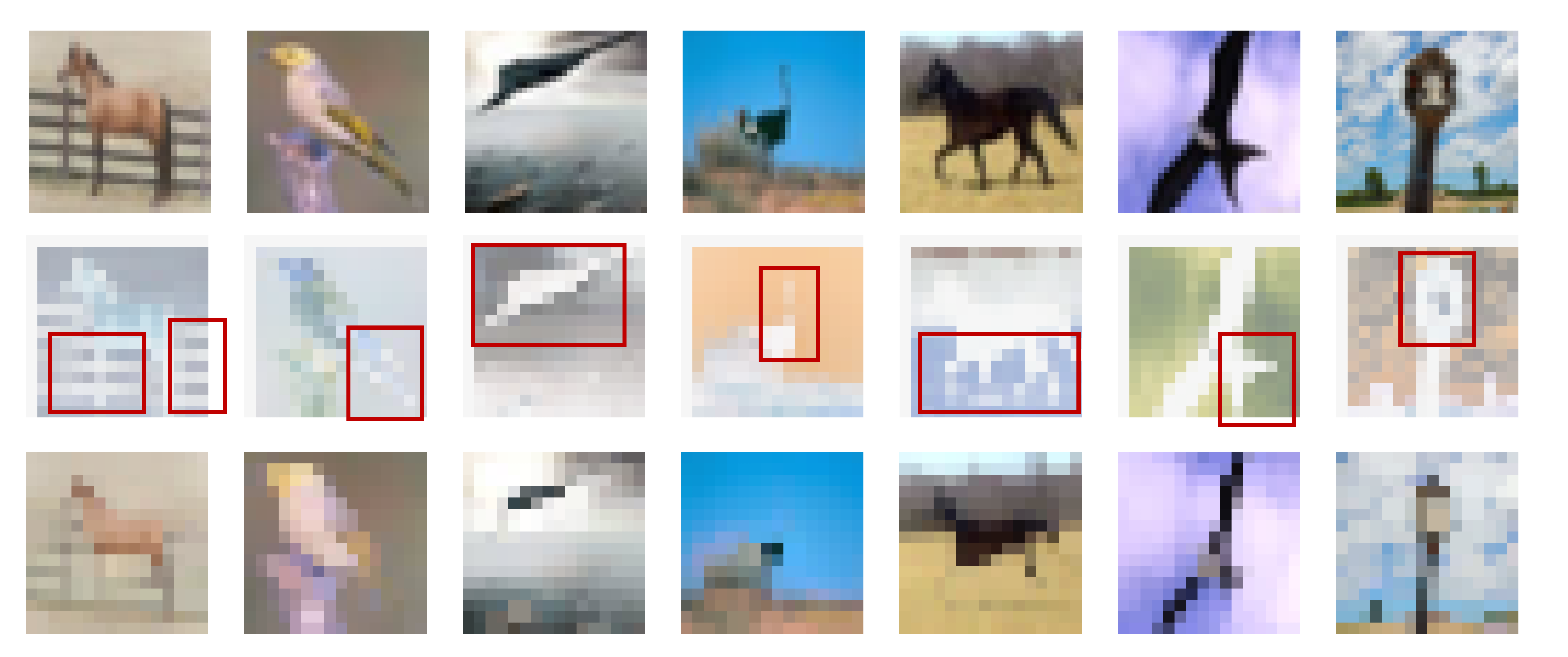
Figure 16: Visualization of images after different downsampling methods on CIFAR-10. Top: Original images. Middle: Quantum Downsampling (Ours). Bottom: Max pooling. Both have kernel size to be $3\times 3$, stride to $2$, and padding to $1$.

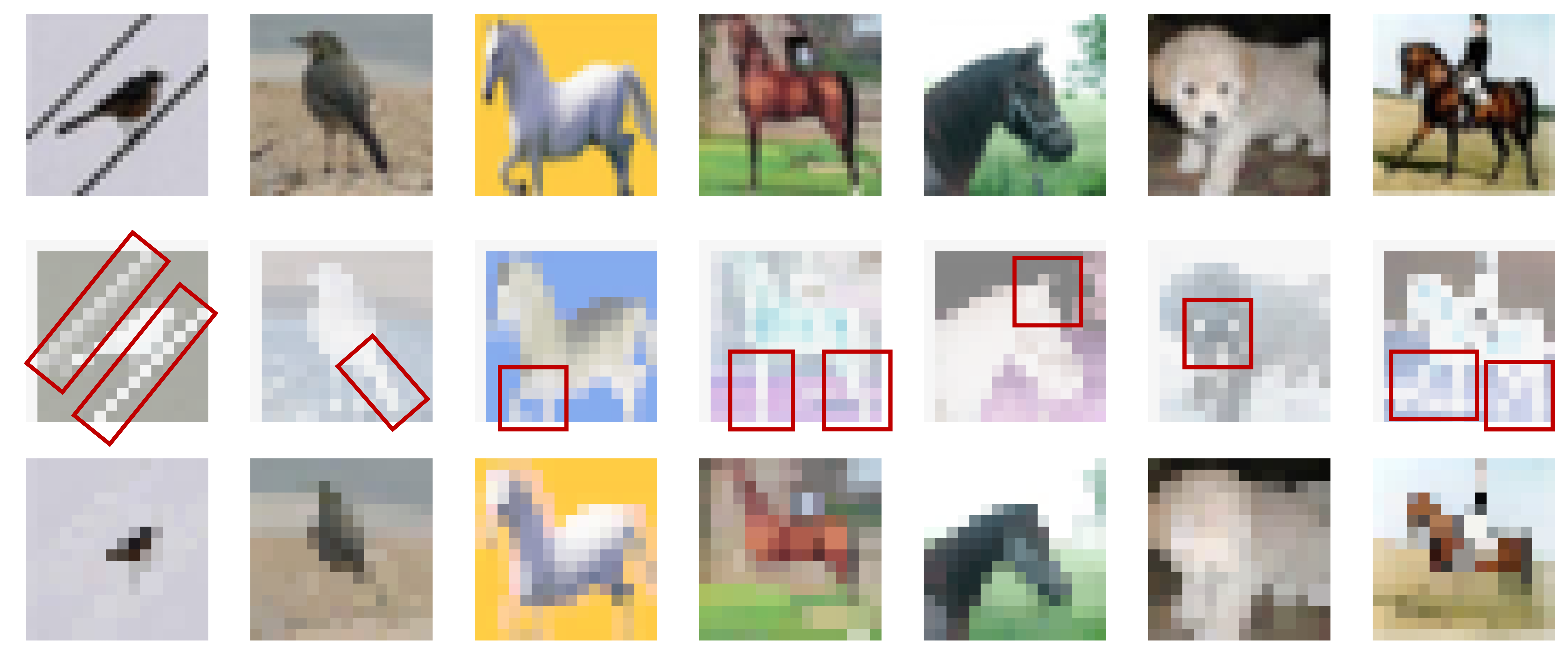
Figure 17: Visualization of images after different downsampling methods on CIFAR-10. Top: Original images. Middle: Quantum Downsampling (Ours). Bottom: Max pooling. Both have kernel size to be $3\times 3$, stride to $2$, and padding to $1$.

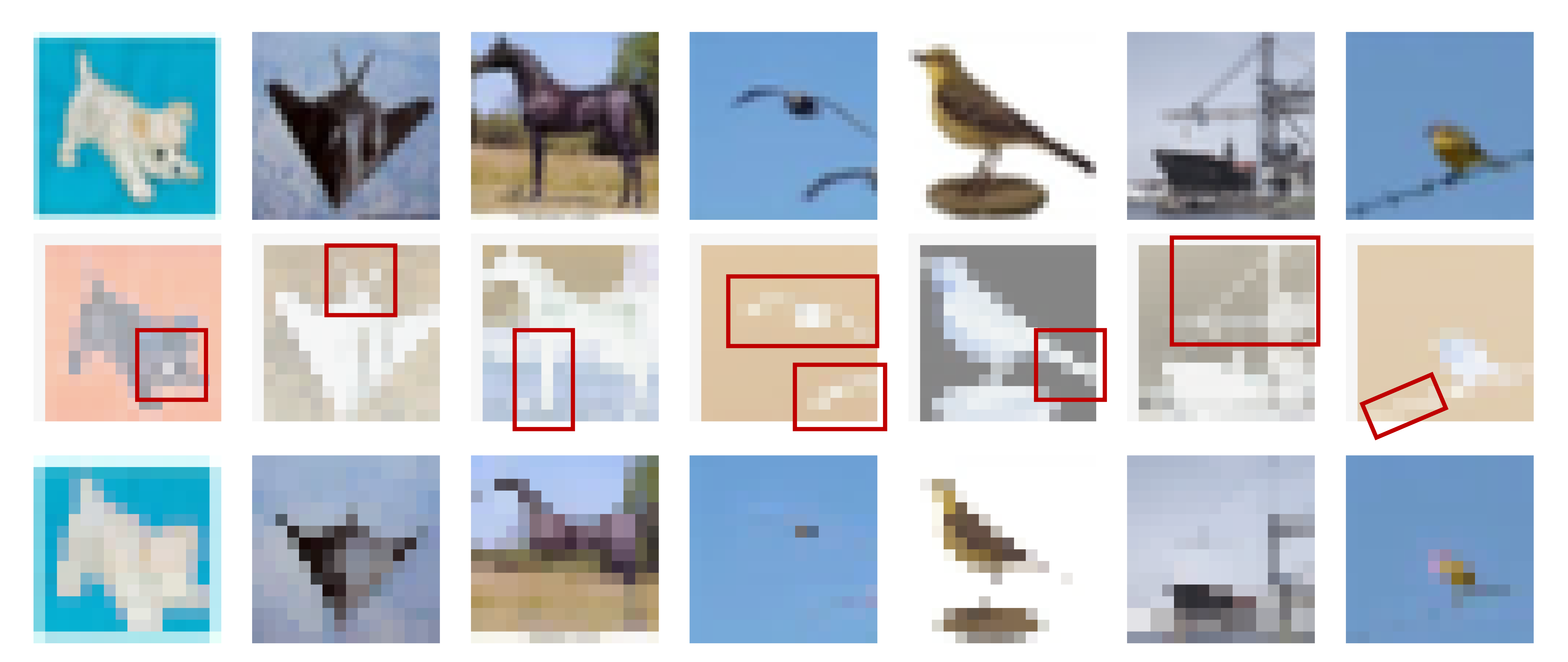
Figure 18: Visualization of images after different downsampling methods on CIFAR-10. Top: Original images. Middle: Quantum Downsampling (Ours). Bottom: Max pooling. Both have kernel size to be $3\times 3$, stride to $2$, and padding to $1$.

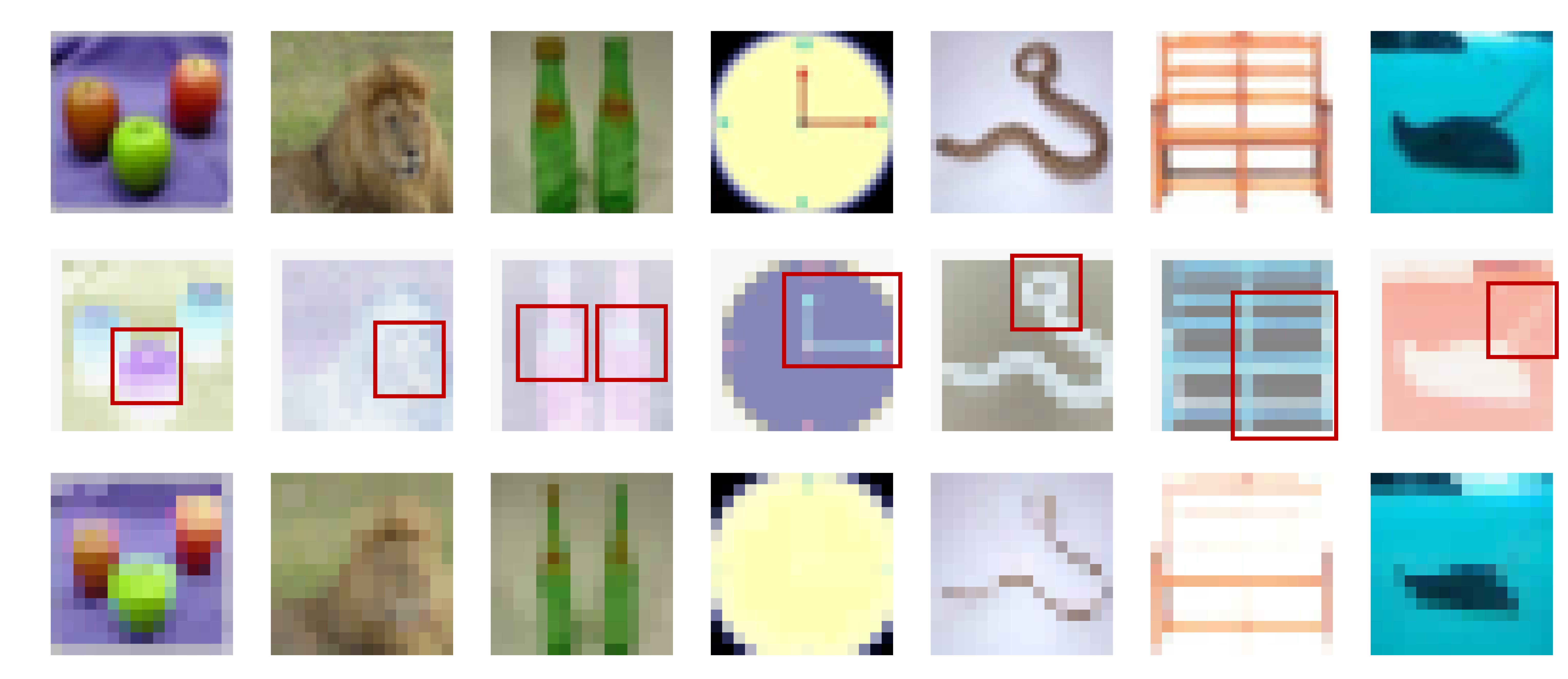
Figure 19: Visualization of images after different downsampling methods on CIFAR-100. Top: Original images. Middle: Quantum Downsampling (Ours). Bottom: Max pooling. Both have kernel size to be $3\times 3$, stride to $2$, and padding to $1$.

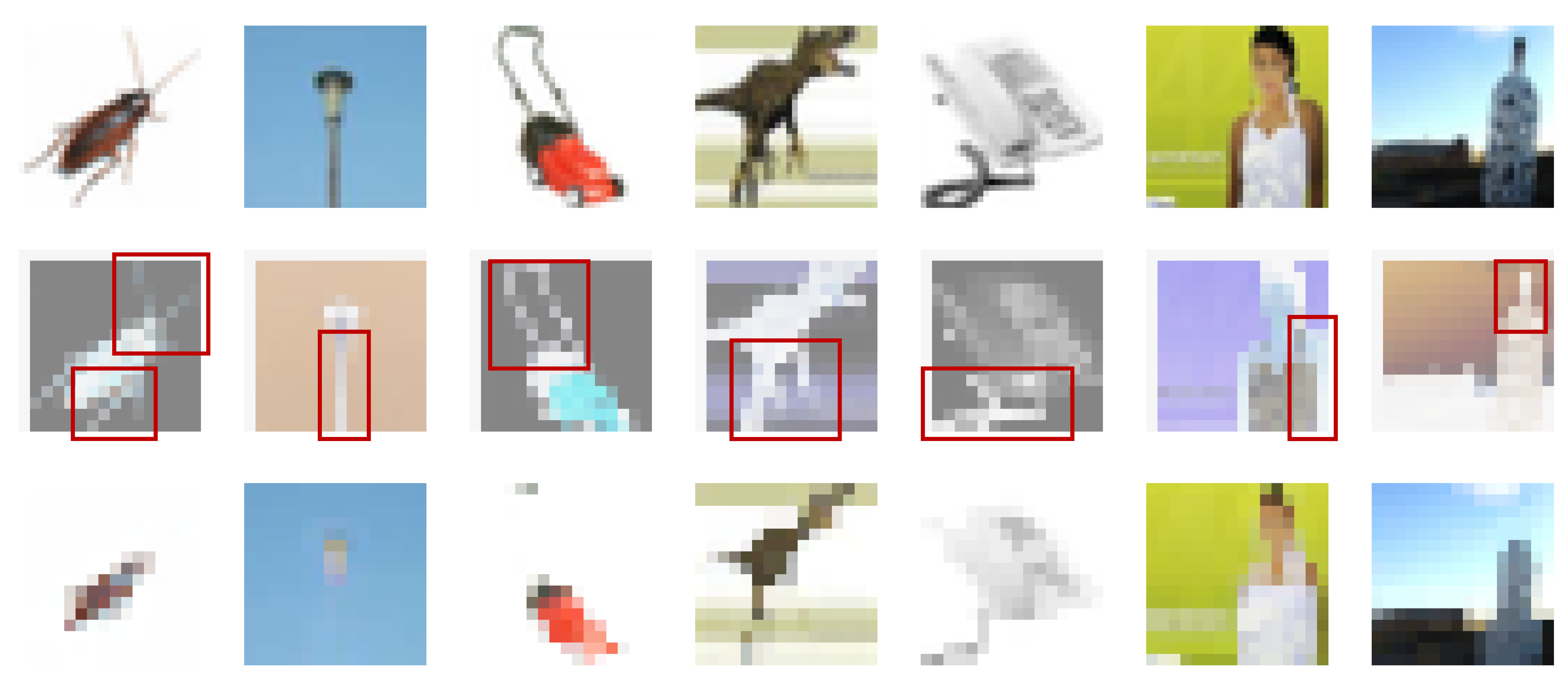
Figure 20: Visualization of images after different downsampling methods on CIFAR-100. Top: Original images. Middle: Quantum Downsampling (Ours). Bottom: Max pooling. Both have kernel size to be $3\times 3$, stride to $2$, and padding to $1$.

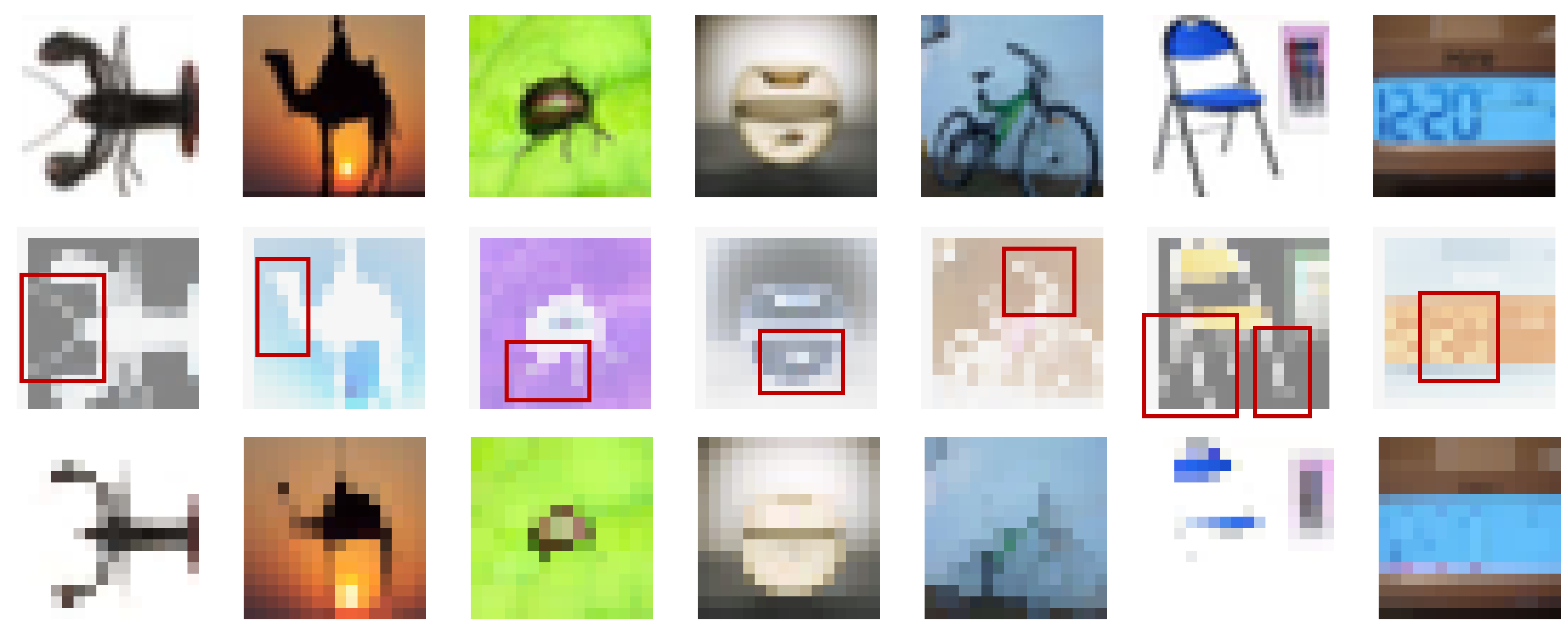
Figure 21: Visualization of images after different downsampling methods on CIFAR-100. Top: Original images. Middle: Quantum Downsampling (Ours). Bottom: Max pooling. Both have kernel size to be $3\times 3$, stride to $2$, and padding to $1$.

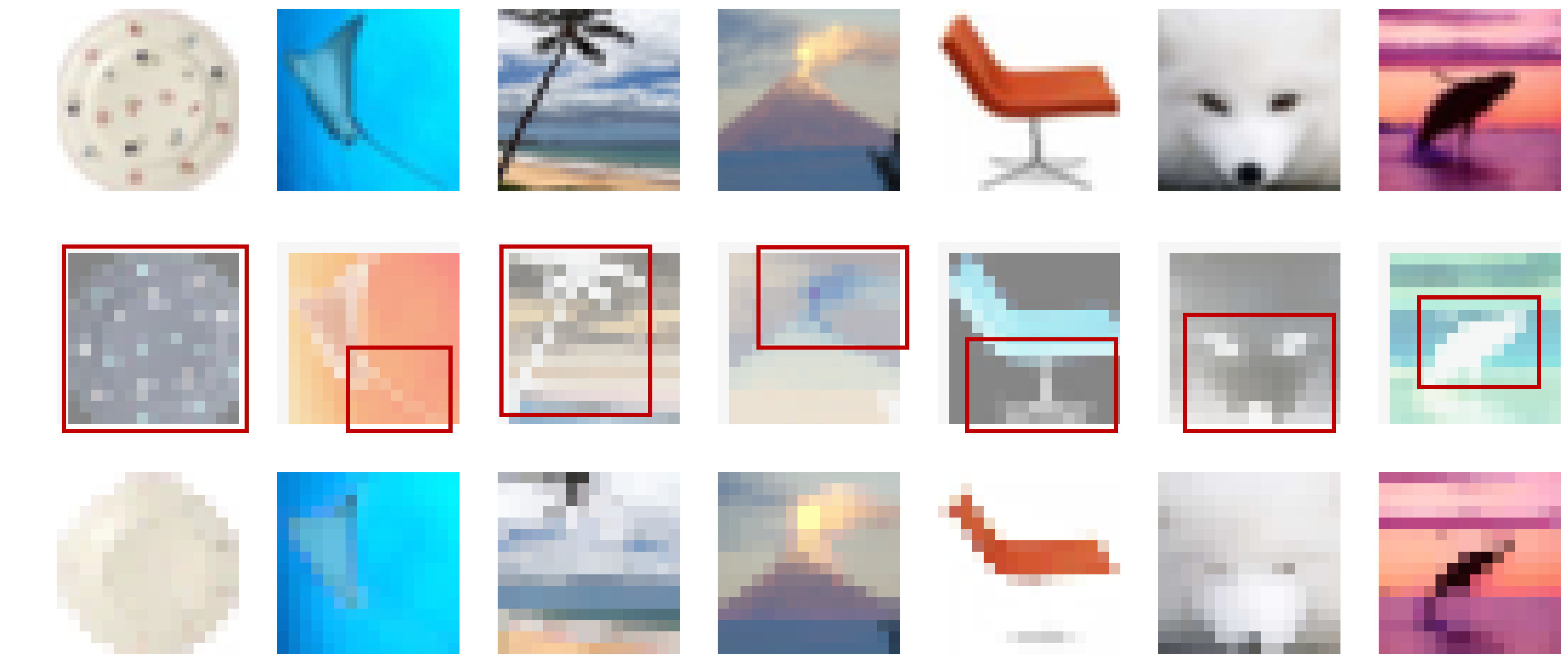
Figure 22: Visualization of images after different downsampling methods on CIFAR-100. Top: Original images. Middle: Quantum Downsampling (Ours). Bottom: Max pooling. Both have kernel size to be $3\times 3$, stride to $2$, and padding to $1$.

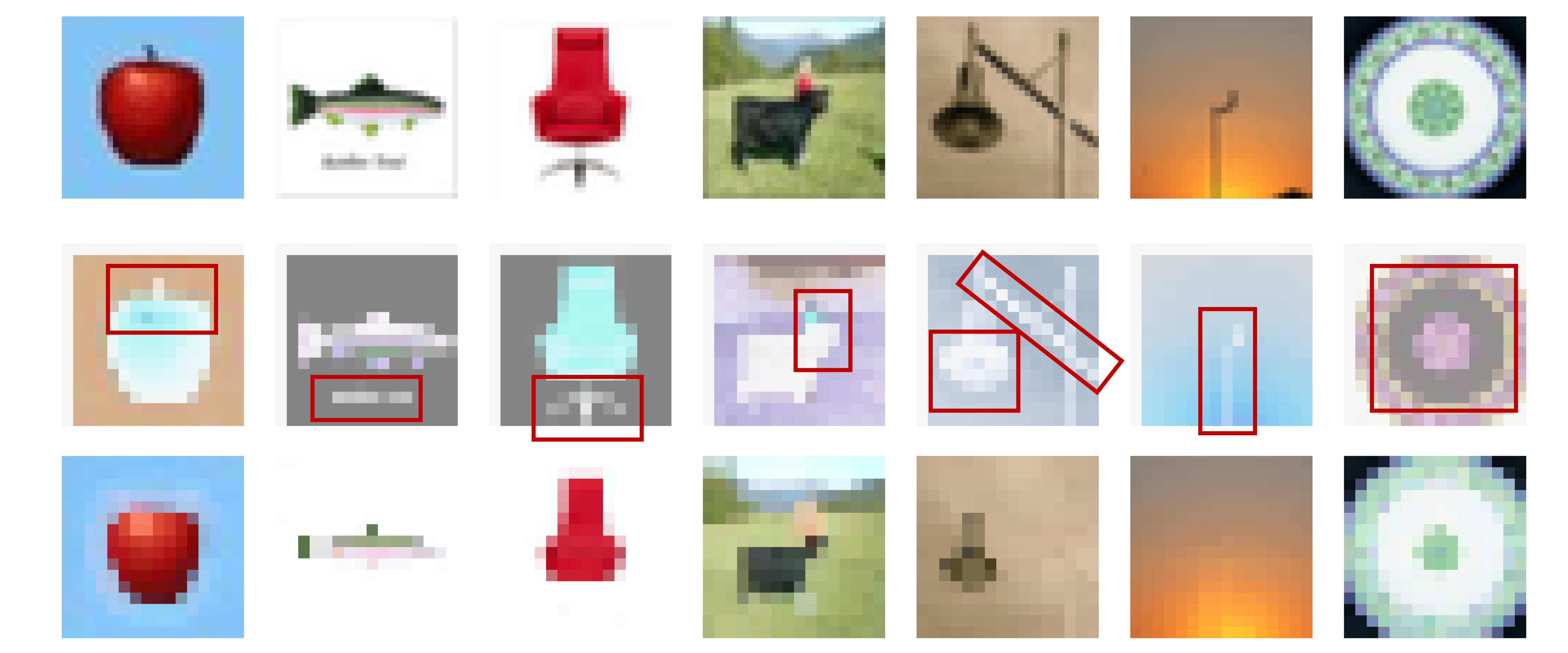
Figure 23: Visualization of images after different downsampling methods on CIFAR-100. Top: Original images. Middle: Quantum Downsampling (Ours). Bottom: Max pooling. Kernel size is to be $3$, stride is to be $2$, and padding is to be $1$.

References

- Arrigoni et al. [2022] Federica Arrigoni, Willi Menapace, Marcel Benkner, Elisa Ricci, and Vladislav Golyanik. Quantum Motion Segmentation, pages 506–523. 10 2022. ISBN 978-3-031-19817-5. doi: 10.1007/978-3-031-19818-2_29.
- Benedetti et al. [2019] Marcello Benedetti, Erika Lloyd, Stefan Sack, and Mattia Fiorentini. Parameterized quantum circuits as machine learning models. Quantum Science and Technology, 4(4):043001, nov 2019. doi: 10.1088/2058-9565/ab4eb5. URL https://dx.doi.org/10.1088/2058-9565/ab4eb5.
- Benkner et al. [2021] Marcel Seelbach Benkner, Zorah Lähner, Vladislav Golyanik, Christof Wunderlich, Christian Theobalt, and Michael Moeller. Q-match: Iterative shape matching via quantum annealing. 2021 IEEE/CVF International Conference on Computer Vision (ICCV), pages 7566–7576, 2021. URL https://api.semanticscholar.org/CorpusID:233864785.
- Bhatia et al. [2023] Harshil Bhatia, Edith Tretschk, Zorah Lähner, Marcel Seelbach Benkner, Michael Moeller, Christian Theobalt, and Vladislav Golyanik. Ccuantumm: Cycle-consistent quantum-hybrid matching of multiple shapes. In Proceedings of the IEEE/CVF Conference on Computer Vision and Pattern Recognition (CVPR), pages 1296–1305, June 2023.
- Birdal et al. [2021] Tolga Birdal, Vladislav Golyanik, Christian Theobalt, and Leonidas J. Guibas. Quantum permutation synchronization. In Proceedings of the IEEE/CVF Conference on Computer Vision and Pattern Recognition (CVPR), pages 13122–13133, June 2021.
- Boureau et al. [2010] Y-Lan Boureau, Jean Ponce, and Yann LeCun. A theoretical analysis of feature pooling in visual recognition. In Proceedings of the 27th International Conference on International Conference on Machine Learning, ICML’10, page 111–118, Madison, WI, USA, 2010. Omnipress. ISBN 9781605589077.
- Bravyi et al. [2022] Sergey Bravyi, Alexander Kliesch, Robert Koenig, and Eugene Tang. Hybrid quantum-classical algorithms for approximate graph coloring. Quantum, 6:678, March 2022. ISSN 2521-327X. doi: 10.22331/q-2022-03-30-678. URL https://doi.org/10.22331/q-2022-03-30-678.
- Caro et al. [2022] Matthias C Caro, Hsin-Yuan Huang, Marco Cerezo, Kunal Sharma, Andrew Sornborger, Lukasz Cincio, and Patrick J Coles. Generalization in quantum machine learning from few training data. Nature communications, 13(1):4919, 2022.
- Cerezo et al. [2022] Marco Cerezo, Guillaume Verdon, Hsin-Yuan Huang, Lukasz Cincio, and Patrick J. Coles. Challenges and opportunities in quantum machine learning. Nature Computational Science, 2:567 – 576, 2022. URL https://api.semanticscholar.org/CorpusID:252323115.
- Chollet [2016] François Chollet. Xception: Deep learning with depthwise separable convolutions. 2017 IEEE Conference on Computer Vision and Pattern Recognition (CVPR), pages 1800–1807, 2016. URL https://api.semanticscholar.org/CorpusID:2375110.
- Cong et al. [2019] Iris Cong, Soonwon Choi, and Mikhail D. Lukin. Quantum convolutional neural networks. Nature Physics, 15:1273–1278, 2019. doi: 10.1038/s41567-019-0648-8.
- De Leon et al. [2021] Nathalie P De Leon, Kohei M Itoh, Dohun Kim, Karan K Mehta, Tracy E Northup, Hanhee Paik, BS Palmer, Nitin Samarth, Sorawis Sangtawesin, and David W Steuerman. Materials challenges and opportunities for quantum computing hardware. Science, 372(6539):eabb2823, 2021.
- Doan et al. [2022] Anh-Dzung Doan, Michele Sasdelli, David Suter, and Tat-Jun Chin. A hybrid quantum-classical algorithm for robust fitting. 2022 IEEE/CVF Conference on Computer Vision and Pattern Recognition (CVPR), pages 417–427, 2022. URL https://api.semanticscholar.org/CorpusID:246276139.
- Domingo et al. [2023] L. Domingo, M. Djukic, C. Johnson, et al. Binding affinity predictions with hybrid quantum-classical convolutional neural networks. Scientific Reports, 13:17951, 2023. doi: 10.1038/s41598-023-45269-y. URL https://doi.org/10.1038/s41598-023-45269-y.
- Farina et al. [2023] Matteo Farina, Luca Magri, Willi Menapace, Elisa Ricci, Vladislav Golyanik, and Federica Arrigoni. Quantum multi-model fitting. In Proceedings of the IEEE/CVF Conference on Computer Vision and Pattern Recognition (CVPR), pages 13640–13649, June 2023.
- Gkoumas et al. [2021] Dimitris Gkoumas, Qiuchi Li, Shahram Dehdashti, Massimo Melucci, Yijun Yu, and Dawei Song. Quantum cognitively motivated decision fusion for video sentiment analysis. In AAAI Conference on Artificial Intelligence, 2021. URL https://api.semanticscholar.org/CorpusID:231582869.
- Golyanik and Theobalt [2020] Vladislav Golyanik and Christian Theobalt. A quantum computational approach to correspondence problems on point sets. In IEEE/CVF Conference on Computer Vision and Pattern Recognition (CVPR), June 2020.
- Gyongyosi and Imre [2019] Laszlo Gyongyosi and Sandor Imre. A survey on quantum computing technology. Comput. Sci. Rev., 31(C):51–71, feb 2019. ISSN 1574-0137. doi: 10.1016/j.cosrev.2018.11.002. URL https://doi.org/10.1016/j.cosrev.2018.11.002.
- He et al. [2016] Kaiming He, Xiangyu Zhang, Shaoqing Ren, and Jian Sun. Deep residual learning for image recognition. In 2016 IEEE Conference on Computer Vision and Pattern Recognition (CVPR), pages 770–778, 2016. doi: 10.1109/CVPR.2016.90.
- Hu et al. [2017] Jie Hu, Li Shen, Samuel Albanie, Gang Sun, and Enhua Wu. Squeeze-and-excitation networks. 2018 IEEE/CVF Conference on Computer Vision and Pattern Recognition, pages 7132–7141, 2017. URL https://api.semanticscholar.org/CorpusID:140309863.
- Huang et al. [2023] Siwei Huang, Yan Chang, Yusheng Lin, and Shibin Zhang. Hybrid quantum–classical convolutional neural networks with privacy quantum computing. Quantum Science and Technology, 8(2):025015, feb 2023. doi: 10.1088/2058-9565/acb966. URL https://dx.doi.org/10.1088/2058-9565/acb966.
- Iandola et al. [2016] Forrest N. Iandola, Matthew W. Moskewicz, Khalid Ashraf, Song Han, William J. Dally, and Kurt Keutzer. Squeezenet: Alexnet-level accuracy with 50x fewer parameters and <1mb model size. ArXiv, abs/1602.07360, 2016. URL https://api.semanticscholar.org/CorpusID:14136028.
- Kandala et al. [2017] Abhinav Kandala, Antonio Mezzacapo, Kristan Temme, et al. Hardware-efficient variational quantum eigensolver for small molecules and quantum magnets. Nature, 549:242–246, 2017. doi: 10.1038/nature23879.
- Lecun et al. [1998] Y. Lecun, L. Bottou, Y. Bengio, and P. Haffner. Gradient-based learning applied to document recognition. Proceedings of the IEEE, 86(11):2278–2324, 1998. doi: 10.1109/5.726791.
- LeCun et al. [1989] Yann LeCun, Bernhard Boser, John Denker, Donnie Henderson, R. Howard, Wayne Hubbard, and Lawrence Jackel. Handwritten digit recognition with a back-propagation network. In D. Touretzky, editor, Advances in Neural Information Processing Systems, volume 2. Morgan-Kaufmann, 1989. URL https://proceedings.neurips.cc/paper_files/paper/1989/file/53c3bce66e43be4f209556518c2fcb54-Paper.pdf.
- Li and Ghosh [2020] Junde Li and Swaroop Ghosh. Quantum-soft qubo suppression for accurate object detection. In Computer Vision – ECCV 2020: 16th European Conference, Glasgow, UK, August 23–28, 2020, Proceedings, Part XXIX, page 158–173, Berlin, Heidelberg, 2020. Springer-Verlag. ISBN 978-3-030-58525-9. doi: 10.1007/978-3-030-58526-6_10. URL https://doi.org/10.1007/978-3-030-58526-6_10.
- Li et al. [2019] Qiuchi Li, Benyou Wang, and Massimo Melucci. CNM: An interpretable complex-valued network for matching. In Jill Burstein, Christy Doran, and Thamar Solorio, editors, Proceedings of the 2019 Conference of the North American Chapter of the Association for Computational Linguistics: Human Language Technologies, Volume 1 (Long and Short Papers), pages 4139–4148, Minneapolis, Minnesota, June 2019. Association for Computational Linguistics. doi: 10.18653/v1/N19-1420. URL https://aclanthology.org/N19-1420.
- Li et al. [2021] Qiuchi Li, Dimitris Gkoumas, Alessandro Sordoni, Jianyun Nie, and Massimo Melucci. Quantum-inspired neural network for conversational emotion recognition. In AAAI Conference on Artificial Intelligence, 2021. URL https://api.semanticscholar.org/CorpusID:235363769.
- McClean et al. [2016] Jarrod R McClean, Jonathan Romero, Ryan Babbush, and Alán Aspuru-Guzik. The theory of variational hybrid quantum-classical algorithms. New Journal of Physics, 18(2):023023, feb 2016. doi: 10.1088/1367-2630/18/2/023023. URL https://dx.doi.org/10.1088/1367-2630/18/2/023023.
- Meli et al. [2022] Natacha Kuete Meli, Florian Mannel, and Jan Lellmann. An iterative quantum approach for transformation estimation from point sets. In 2022 IEEE/CVF Conference on Computer Vision and Pattern Recognition (CVPR), pages 519–527, 2022. doi: 10.1109/CVPR52688.2022.00061.
- Nielsen and Chuang [2010] Michael A. Nielsen and Isaac L. Chuang. Quantum Computation and Quantum Information: 10th Anniversary Edition. Cambridge University Press, 2010.
- Pan et al. [2023] Hongyi Pan, Xin Zhu, Salih Atici, and Ahmet Enis Cetin. A hybrid quantum-classical approach based on the hadamard transform for the convolutional layer. In Proceedings of the 40th International Conference on Machine Learning, ICML’23. JMLR.org, 2023.
- Perdomo-Ortiz et al. [2017] Alejandro Perdomo-Ortiz, Marcello Benedetti, John Realpe-Gómez, and Rupak Biswas. Opportunities and challenges for quantum-assisted machine learning in near-term quantum computers. Quantum Science and Technology, 3, 2017. URL https://api.semanticscholar.org/CorpusID:3963470.
- Preskill [2018a] John Preskill. Quantum Computing in the NISQ era and beyond. Quantum, 2:79, August 2018a. ISSN 2521-327X. doi: 10.22331/q-2018-08-06-79. URL https://doi.org/10.22331/q-2018-08-06-79.
- Preskill [2018b] John Preskill. Quantum computing in the nisq era and beyond. Quantum, 2:79, 2018b.
- Robbins [1951] Herbert E. Robbins. A stochastic approximation method. Annals of Mathematical Statistics, 22:400–407, 1951. URL https://api.semanticscholar.org/CorpusID:16945044.
- Silver et al. [2023] Daniel Silver, Tirthak Patel, William Cutler, Aditya Ranjan, Harshitta Gandhi, and Devesh Tiwari. Mosaiq: Quantum generative adversarial networks for image generation on nisq computers. In Proceedings of the IEEE/CVF International Conference on Computer Vision (ICCV), pages 7030–7039, October 2023.
- Simonyan and Zisserman [2014] Karen Simonyan and Andrew Zisserman. Very deep convolutional networks for large-scale image recognition. CoRR, abs/1409.1556, 2014. URL https://api.semanticscholar.org/CorpusID:14124313.
- Tang et al. [2022] Yehui Tang, Kai Han, Jianyuan Guo, Chang Xu, Yanxi Li, Chao Xu, and Yunhe Wang. An image patch is a wave: Phase-aware vision mlp. In Proceedings of the IEEE/CVF Conference on Computer Vision and Pattern Recognition (CVPR), pages 10935–10944, June 2022.
- et al. [2018] Ville Bergholm et al. Pennylane: Automatic differentiation of hybrid quantum-classical computations, 2018.
- Wang et al. [2017] Fei Wang, Mengqing Jiang, Chen Qian, Shuo Yang, Cheng Li, Honggang Zhang, Xiaogang Wang, and Xiaoou Tang. Residual attention network for image classification. In 2017 IEEE Conference on Computer Vision and Pattern Recognition (CVPR), pages 6450–6458, 2017. doi: 10.1109/CVPR.2017.683.
- Wang et al. [2023] Jinchen Wang, Mohamed I. Ibrahim, Isaac B. Harris, Nathan M. Monroe, Muhammad Ibrahim Wasiq Khan, Xiang Yi, Dirk R. Englund, and Ruonan Han. 34.1 thz cryo-cmos backscatter transceiver: A contactless 4 kelvin-300 kelvin data interface. In 2023 IEEE International Solid-State Circuits Conference (ISSCC), pages 504–506, 2023. doi: 10.1109/ISSCC42615.2023.10067445.
- Xie et al. [2016] Saining Xie, Ross B. Girshick, Piotr Dollár, Zhuowen Tu, and Kaiming He. Aggregated residual transformations for deep neural networks. 2017 IEEE Conference on Computer Vision and Pattern Recognition (CVPR), pages 5987–5995, 2016. URL https://api.semanticscholar.org/CorpusID:8485068.
- Yang and Sun [2022] Yuan-Fu Yang and Min Sun. Semiconductor defect detection by hybrid classical-quantum deep learning. In Proceedings of the IEEE/CVF Conference on Computer Vision and Pattern Recognition (CVPR), pages 2323–2332, June 2022.
- Zaech et al. [2022] Jan-Nico Zaech, Alexander Liniger, Martin Danelljan, Dengxin Dai, and Luc Van Gool. Adiabatic quantum computing for multi object tracking. 2022 IEEE/CVF Conference on Computer Vision and Pattern Recognition (CVPR), pages 8801–8812, 2022. URL https://api.semanticscholar.org/CorpusID:246904708.
- Zhang et al. [2023] Jie Zhang, Yongshan Zhang, and Yicong Zhou. Quantum-inspired spectral-spatial pyramid network for hyperspectral image classification. In Proceedings of the IEEE/CVF Conference on Computer Vision and Pattern Recognition (CVPR), pages 9925–9934, June 2023.
- Zoph et al. [2017] Barret Zoph, Vijay Vasudevan, Jonathon Shlens, and Quoc V. Le. Learning transferable architectures for scalable image recognition. 2018 IEEE/CVF Conference on Computer Vision and Pattern Recognition, pages 8697–8710, 2017. URL https://api.semanticscholar.org/CorpusID:12227989.