Neural Adaptive Control of Vehicle Lateral Dynamics
Abstract
We address the problem of stable and robust control of vehicles with lateral error dynamics for the application of lane keeping. Lane departure is the primary reason for half of the fatalities in road accidents, making the development of stable, adaptive and robust controllers a necessity. Traditional linear feedback controllers achieve satisfactory tracking performance, however, they exhibit unstable behavior when uncertainties are induced into the system. Any disturbance or uncertainty introduced to the steering-angle input can be catastrophic for the vehicle. Therefore, controllers must be developed to actively handle such uncertainties. In this work, we introduce a Neural Adaptive controller (Neural-L1) which learns the uncertainties in the lateral error dynamics of a front-steered Ackermann vehicle and guarantees stability and robustness. Our contributions are threefold: i) We extend the theoretical results for guaranteed stability and robustness of conventional Adaptive controllers to Neural-L1; ii) We implement a Neural-L1 for the lane keeping application which learns uncertainties in the dynamics accurately; iii) We evaluate the performance of Neural-L1 on a physics-based simulator, PyBullet, and conduct extensive real-world experiments with the F1TENTH platform to demonstrate superior reference trajectory tracking performance of Neural-L1 compared to other state-of-the-art controllers, in the presence of uncertainties. Our project page, including supplementary material and videos, can be found at https://mukhe027.github.io/Neural-Adaptive-Control/
Index Terms:
Adaptive control; Autonomous vehicles; Lateral error dynamics; Robust control.I Introduction
Safety critical systems are prevalent in the transportation industry, especially in the aerospace sector. Therefore, the focus has always been on automating flight control systems because of the underlying complexities of flying an aircraft [1, 2, 3]. On the contrary, in the automotive sector, road vehicles have traditionally been driven manually, primarily dependent on a human making decisions behind the wheel. For automotive systems, the lower level vehicle control system relies on conventional controllers such as the linear state-feedback controller (LF) [4]. However, with recent surge in interest for developing autonomous road vehicles, there is a need for more reliable control systems that are robust to induced uncertainties.
Federal Highway Administration has stated that from 2016 to 2018 an average of 19,158 fatalities resulted from roadway departures, which is 51 percent of all traffic fatalities in the United States [5]. Lane departures are identified to be the number one cause of fatal accidents in the United States by the National Highway Transportation Safety Administration. Thus, there has been significant investment in research in industry as well as in academia for developing systems that recognize and identify accidental lane departures of vehicles [4, 6]. In this direction, some of the research thrusts are: lane departure warning systems (LDWS), lane keeping systems (LKS) and yaw stability control systems. We particularly focus on LKS in this paper and propose to develop not just a stable controller but also an adaptive controller which is robust to uncertainties induced into a system in the form of sensor noise, control signal disturbances and external obstacles on road.
With the need for certifying advanced adaptive flight critical systems emerging rapidly, the seminal work by Hovakimyan et al. [1] introduces adaptive controller (L1adap). L1adap [7, 8, 9, 10, 11, 12, 13] is a class of control system which is inherently derived from the traditional class of adaptive controllers, Model Reference Adaptive Controllers (MRAC) [14, 15, 16] and the State Predictor-based MRAC [17]. Beyond the traditional properties of guaranteed stability and adaptiveness of MRAC type controllers, L1adap provides robustness guarantees to uncertainties induced into the system dynamics. In this paper, we show that the performance of traditional L1adap[1] can be further enhanced with the help of neural network. Deep-MRAC in [18] has demonstrated that the controller performance of traditional MRAC is further improved by using neural network to derive the adaptive laws that learn the uncertainties better, instead of using conventional adaptive laws of MRAC to estimate the true uncertainties. Therefore, we present the implementation of a modified L1adap, Neural Adaptive controller (Neural-L1), where the adaption law is learned by learning the weights of neural network using the framework in [18], and then appended to the adaptive laws derived from the conventional theory of L1adap in [1]. Further, we extend the proof for stability and robustness of the L1adap [1] with this new neural network framework to Neural-L1. Finally, we evaluate the performance of Neural-L1 for a lane-keeping application using a physics-based simulation of the F1TENTH front-steered Ackermann vehicle as well as on a real F1TENTH vehicle. Our evaluations show that the proposed Neural-L1 is robust and stable in the presence of uncertainties, whereas other existing controllers such as the LF [4] and the Deep-MRAC controller from [18] exhibit unstable behavior and have a deteriorating tracking performance. When the tracking performance of our proposed controller is compared with that of the conventional L1adap, the use of neural network to learn the residual uncertainty enhances the tracking performance of our proposed controller. To summarise, our contributions are threefold: i) We extend the theoretical results for guaranteed stability and robustness of conventional L1adap to Neural-L1; ii) We implement a Neural-L1 for lane keeping application of front-steered Ackermann vehicles which uses neural network to learn induced uncertainties in the system dynamics; iii) We evaluate the performance of Neural-L1 on a physics-based simulator, PyBullet, and conduct extensive real-world experiments with the F1TENTH platform to demonstrate superior reference trajectory tracking performance of Neural-L1 compared to other state-of-the-art controllers. For a rigorous evaluation of all controllers, we externally induce sensor noise, control signal disturbance and place physical obstacles in environment. Neural-L1 exhibits stability and robustness to induced noise and disturbance to achieve successful tracking of arbitrary reference trajectories.
The rest of the paper is organized as follows. Related work is summarized in Section II. The formal problem formulation is given in Section III. In Section IV, we provide extensive details of the stability theory behind Neural-L1. Finally, we provide simulation and experimental results with F1TENTH in Sections V and VI and conclude the paper in Section VII.
II Related Work
The works [19, 20, 21, 22, 23] are some of the initial efforts that discuss control methods for maintaining stability in road vehicles for prevention of rollover and lateral control of front-steered vehicles. With respect to applications such as LKS and LDWS, lateral control of vehicle is of importance. [24, 25, 26, 27, 28, 29, 30, 31] are works which discuss the application of stable lateral control in road vehicles and [32, 33, 34] are more recent works that address the problem of stable steering control in vehicles. In [25], the authors provide one of the first studies of application of vision-based systems in lateral control of vehicles. In work [26], authors develop a two-part trajectory planning algorithm which consists of the steering planning and velocity planning for a four-wheeled steering vehicle. However, none of these works address the issue of controller stability, adaptiveness and robustness in the presence of external factors such as sensor noise, control signal disturbance or physical obstacles on road.
With the interest growing in developing LKS and LDWS technologies, there is a need for controllers that can adapt to uncertainties induced externally into the system. Most Proportional-Integral-Derivative (PID) controllers should be sufficient to implement LKS and LDWS systems as demonstrated in these works [35, 36, 37]. In this regard, linear state-feedback controllers such as PID controllers are usually the primary choice due to their fairly robust nature and the ease of implementation on real systems, but since control systems are prone to uncertainties being induced from the environment, PID controllers are not capable of adapting in real-time to these uncertainties efficiently. Therefore, this naturally drives the interest for developing adaptive controllers. Adaptive controllers have been around for a while [38, 39, 40, 41], but they are primarily implemented for highly safety-critical aerospace systems [42, 18]. In [42], the authors, for the first time, implement an MRAC for the flight control system of F-16 aircraft. The work in [18] is relatively new which shows stable control of aerial vehicles, where the adaptive laws of the MRAC are learned using a neural network. The MRAC framework is adaptive and stable, but it is not robust with respect to uncertainties in the dynamics of the system. In this paper, we adopt the neural network architecture from [18] and apply it to a traditional L1adap to account for robustness. The key feature of L1adap [1] architecture is that it guarantees robustness in the presence of fast adaptation, which leads to uniform performance bounds both in transient and steady-state operation.
In the recent works [43, 44], the authors demonstrate the augmentation of L1adap to other conventional controllers. The work [43] augments L1adap to a geometric controller for control of quadrotors. The authors demonstrate that the robustness characteristic of L1adap handles non-linear uncertainties induced into the system, whereas [44] augments the same with a feedforward-feedback control system and learns a stable controller for adaptive trajectory tracking of unfeasible trajectories by quadrotors. None of these works address the LKS application. In [45], the authors provide only simulation results corroborating the characteristics of stability, robustness and adaptability claimed by the seminal work [1] for the application of lane keeping using the lateral error dynamics in [4].
III Problem Formulation
In this section, we review the theory behind the front-steered Ackermann vehicle lateral error dynamics from [4] and the neural network approach we adopt from [18].
III-A Vehicle Lateral Error Dynamics
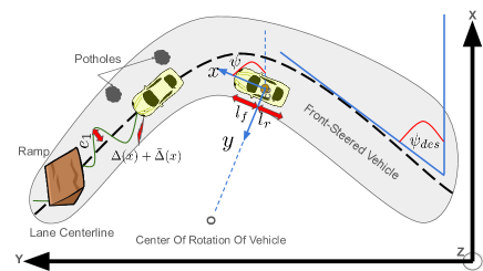
Fig. 1 is a depiction of a simplified linear two-degrees of freedom (2-DOF) bicycle model of the vehicle lateral dynamics derived in [4]. 2-DOF is represented by , the vehicle yaw angle, and , the lateral position with respect to the center of the rotation of the vehicle . The yaw angle is considered as the angle between horizontal vehicle body frame axis of the vehicle, , and the global horizontal axis, . The constant longitudinal velocity of the vehicle at its center of gravity () is denoted by and the mass of the vehicle is denoted by . The distances of the front and rear axles from the are shown by , , respectively, and the front and rear tire cornering stiffness are denoted by and , respectively. The steering angle is denoted by which also serves as the control signal when a controller is implemented and the yaw moment of inertia of the vehicle is denoted by . Considering the lateral position, yaw angle, and their derivatives as the state variables, and using the Newton’s second law for the motion along the vehicle body frame , the state space model of lateral vehicle dynamics is derived in [4].
The error dynamics is written with two error variables : , which is the distance between the of the vehicle from the center line of the lane; , which is the orientation error of the vehicle with respect to the desired yaw angle . Assuming the radius of the road is , the rate of change of the desired orientation of the vehicle can be defined as . The tracking or lane keeping objective of the lateral control problem is expressed as a problem of stabilizing the following error dynamics at the origin.
| (1) |
Therefore, the above state-space form in (III-A) can be represented in the general state space form as in (2)
| (2) |
where , is a state vector, , is the control input which in this case is the steering angle . The elements of , matrices are generally considered known, but in our case we obtain the elements of matrices from our system identification work [46] and we assume pair is controllable.
III-B Deep Neural Networks (DNN) Architecture
In this paper, we incorporate the DNN architecture from [18] with the purpose of extracting relevant features of the system uncertainties, which otherwise is not trivial to obtain without the limits on the domain of operation. The idea in machine learning is that a given function can be encoded with weighted combinations of feature vector , s.t , and a vector of ideal weights s.t . DNNs utilize composite functions of features arranged in a directed acyclic graph, i.e. where ’s are the layer weights. In this regard, we implement a dual time-scale learning scheme, same as in [18], to learn the uncertainties in real time. In the dual time-scale scheme, the weights of the outermost layers are adapted in real time using a generative network, whereas the weights of the inner layers are adapted using batch updates. Unlike the conventional neural network training where the true target values are available for every input , in this paper, true system uncertainties as the labeled targets are not available for the network training. Therefore, we use part of the network itself (the last layer) with pointwise weight updated according to the adaptive laws of L1adap as the generative model for the data. The generative model uncertainty estimates along with inputs make the training data set . The adopted DNN architecture is shown in green in Fig. 2. As shown in Fig. 2, the adopted DNN architecture is appended to the adaptive laws learned by the traditional L1adap in red. The reader is referred to [18] for extensive detail on the network architecture and the results evaluating the DNN training, testing and validation performances.
III-C Problem Statement
In this subsection, we state our problem. We remind the reader that in general conventional stable controllers exist for the LKS application, but with increase in interest for autonomy, development of not only stable, but robust and adaptive controllers is a necessity. Thus, in this work, we place emphasis on taking an existing stable, robust and adaptive controller, the L1adap, extend this controller’s theory while incorporating learning mechanisms of neural network to improve the controller’s performance to guarantee to maintain the controller’s stability, adaptiveness and robustness properties and apply the modified L1adap controller to LKS applications.
Problem 1.
Given the lateral error dynamics in (III-A) for front-steered Ackermann vehicles, determine a stable, adaptive and robust control law in the form of steering angle control signal such that the front-steered vehicle maintains the lane on a road with constant radius while adapting to unknown, unmodeled external disturbances such as sensor noise, control signal disturbance and physical obstacles on road, in real time. The adaptive properties of the controller can be further enhanced by incorporating learning mechanisms of neural network.
The above problem is especially difficult when the nature of the disturbance induced into the system is unknown and hard to model. Existing adaptive controllers derive an adaptive law to learn the disturbance, where using neural network further aids with the learning capability of the controller.
IV System Overview
In this section, we present the stability theory for the Neural-L1 controller. The stability analysis of Neural-L1 is an extension of the stability analysis of L1adap [1]. After augmenting the traditional L1adap controller with the DNN framework from [18] to derive the Neural-L1 controller, the extension of the stability analysis of L1adap becomes non-trivial. Therefore, in this section, we outline the steps as well as provide theoretical results for a complete stability analysis of our proposed Neural-L1 controller. Fig. 2 shows the complete Neural-L1 architecture.
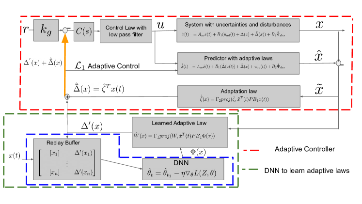
We would like to emphasize that our controller architecture of Neural-L1 is different from the controller architecture of Deep-MRAC in [18]. This is because we append the adaptive laws learned by the DNN framework to the adaptive laws derived by the L1adap [1] controller, unlike in Deep-MRAC [18] where the adaptive laws learned by the DNN framework replace the adaptive laws derived from a traditional MRAC [16] controller. The addition of the DNN based adaptive laws to the adaptive laws derived by L1adap is indicated with an yellow arrow in Fig 2.
The stability analysis of Neural-L1 consists of the following steps. First, we will define an ideal closed-loop reference system with control law . We will then use the norm condition to show that is uniformly bounded in Lemma 1. Next, we will analyse the transient and steady state performance of our controller by first defining the error dynamics as , then presenting results of uniform boundedness of and convergence to lower bound in Lemma 2 and Lemma 3, respectively. The error dynamics is derived as the plant and state predictor error dynamics. We prove in Lemma 3 by proving that the state of the predictor remains bounded. Finally, using the results from Lemma 2 and Lemma 3, we show the main results in Theorem 1 proving uniform boundedness of and . The results in Theorem 1 imply that by selecting the right parameters for the static feedback gain , the Bounded Input, Bounded Output (BIBO)-stable and strictly proper transfer function of the filter and the adaptation gain , we can ensure a desirable response out of the reference system and expect the plant states to approach the reference system closely. We conclude this section discussing the proof for Lyapunov stability of the complete controller after the augmentation of the DNN framework.
IV-A Adaptive Control (L1adap) Architecture
Consider the total adaptive control law , consisting of linear feedback component, , and the adaptive control component
| (3) |
where renders Hurwitz, while is the adaptive component, to be defined shortly. The static feedback gain , with the control law in (3) substituted in (2), leads to the following closed-loop system:
| (4) |
where , which follows the relation from traditional adaptive controller derivation. We refer the reader to [17] for background reading on the theory of State Predictor-based MRAC as it forms the basis of derivation for the theory of L1adap. Consequently, for a linearly parameterized system in (IV-A), we consider the state predictor as
| (5) |
where is the state of the predictor and are the estimates of the unknown parameter , and .
The total true uncertainty is unknown111Note that dependence on time will only be shown when introducing new concepts or symbols. Subsequent usage will drop these dependencies for clarity of presentation., but it is assumed to be continuous over the compact set . In this paper, we use the adaptive laws from the traditional L1adap to learn part of the total true uncertainty, , and we use the augmented DNN framework to learn the residual uncertainty, . We use a DNN framework to represent a function when the basis vector is unknown. Using DNNs, a non-linearly parameterized network estimate of the uncertainty can be written as , where are network weights for the final layer and , is a dimensional feature vector which is a function of the inner layer weights, activations and inputs. The basis vector is considered to be Lipschitz continuous to ensure the existence and uniqueness of the solution.
IV-B Adaptive Control Law
We now derive in (3). We know that the form of satisfies the matching conditions such that , which is a typical form of the full state feedback controller. Further, we would like to choose such that it cancels out , however, since and are unknown, we estimate .
From [1], we know that L1adap framework is implemented using a low-pass filter of the form , where is a BIBO-stable and stricly proper transfer function with DC gain , and its state space realization assumes zero initialization. Therefore, the control law term is given by
| (6) |
where , , are the Laplace transforms of reference signal , , and , and the reference signal gain . Furthermore, the reference signal is assumed to be bounded, piece wise continuous, with quantifiable transient and steady-state performance bounds.
In this paper, we are using an online DNN framework similar to [18] to estimate residual uncertainty, where the true estimates of the labeled pairs of state and true residual uncertainty are needed. To achieve the asymptotic convergence of the predictive model tracking error to zero, we substitute the DNN estimate in the controller , where
| (7) |
We now state Assumption 1 from [18].
Assumption 1.
(from [18]) Appealing to the universal approximation of Neural networks we have that, for every given basis functions there exists unique ideal weights and such that the following approximation holds
| (8) |
Fact 1.
(from [18]) The network approximation error is upper bounded, s.t. , and can be made arbitrarily small given sufficiently large number of basis functions.
Next, we discuss the estimation method of the unknown true network parameters . The unknown true network parameters are estimated using the estimation or the adaptive law given as
| (9) |
where is the prediction error, is the adaptation gain, and solves the algebraic Lyapunov equation for arbitrary symmetric . The projection is confined to the set . With the neural network-based adaptive law stated in (9), the adaptation law from a L1adap can be represented as
| (10) |
Then, taking the Laplace transform of , the adaptive control signal looks like
| (11) |
Now that the L1adap is defined using the relationships in (3), (IV-A), (6) and (9), with and , it must satisfy the -norm condition given by
| (12) |
where , , . However, in this work, since we are using neural networks to learn the residual uncertainty parameter, we have an additional norm condition to satisfy
| (13) |
where . Therefore, we define the following nonadaptive version of the adaptive control system, also known as the closed-loop reference system of the class of systems in (2)
| (14) |
Next, we provide the first theoretical result in Lemma 1 where we signify the importance of the condition, such that can be shown to be uniformly bounded.
Lemma 1.
If , then the system in (IV-B) is bounded-input bounded-state stable with respect to the reference signal and .
Proof.
From the definition of the closed-loop reference system in (IV-B) , it follows
| (15) |
where , is the Laplace transform of . Recalling the fact that and are proper BIBO-stable transfer functions, it follows from (IV-B) that for , the following bounds hold:
| (16) |
Since is Hurwitz, is uniformly bounded. Thus, using the relation in (12) we can imply that
| (17) |
Consequently,
| (18) |
Since and are uniformly bounded, and (IV-B) holds uniformly for , is uniformly bounded. This completes the proof. Note that the true uncertainty is assumed to be continuous and bounded over a compact domain , which implies is also bounded. ∎
IV-C Transient and Steady-State Performance
For the error , the error dynamics , using (IV-A) and (IV-A) can be written as
| (19) |
where . Further, we let , with being its Laplace transform and with being its Laplace transform. Therefore, the error dynamics in frequency domain can be re-written as
| (20) |
where is the Laplace transform of . Before we present the uniform boundedness result of in Lemma 2, we state Assumption 2
Assumption 2.
(from [18]) For uncertainty parameterized by unknown true weights and known nonlinear , the ideal weight matrix is assumed to be upper bounded s.t. .
As done in [18], we will prove the following lemma under switching feature vector assumption.
Lemma 2.
The prediction error is uniformly bounded.
Proof.
The feature vectors belong to a function class characterized by the inner layer network weights s.t . Using the same manipulation process in Theorem 1 in [18], we will prove the Lyapunov stability under the assumption that inner layer of DNN presents us a feature which results in the worst possible approximation error compared to network with features before switch.
For this purpose, we will denote as feature before switch and as the feature after switch. We define the error as
| (21) |
Using Fact 1, we can upper bound as . Thus, by adding and subtracting the term , we can rewrite the error dynamics (19)
| (22) |
Then by applying Assumption 1, there exists . Therefore, we can replace by in (19) to obtain
| (23) |
Thus, we consider the following Lyapunov function
| (24) |
Now taking the time derivative of the Lyapunov function in (24), we get as
| (25) |
where and . Hence, Lyapunov stability is obtained outside compact neighborhood of the origin , for some sufficiently large where we can show a lower bound on as
| (26) |
Now, what remains is to show that is upper bounded. In this direction, since and in the vicinity of the compact neighborhood of the origin , it follows that
| (27) |
The projection operators222Definition of projection operators can be found in [1]. with Assumption 2 ensure that the error parameters and are bounded and so we have
| (28) |
which leads to the following upper bound:
| (29) |
Since , and this bound is uniform, the bound above yields
| (30) |
which holds for every
∎
Notice that the bounds on are obtained independent of the control term . This implies that both and can diverge at the same rate, maintaining a uniformly bounded error between the two. Therefore, the result in Lemma 3 will prove that using the control law , the state of the predictor remains bounded and consequently leads to asymptotic convergence of the tracking error to the lower bound .
Lemma 3.
Proof.
To prove asymptotic convergence of to , one needs to ensure that with is uniformly bounded. Therefore, we have
| (31) |
where and is the Laplace transform, which leads to the following upper bound
| (32) |
Next, applying the triangular relationship for norms to the bound in (30), we have
| (33) |
The projection operators ensure that the error parameters and are bounded , and hence we have . Substituting for yields
| (34) |
Then the bound on and in (IV-C) and (34), with account of the stability conditions in (12) and (13), lead to
| (35) |
Since the bound on the right hand side is uniform, is uniformly bounded. Application of Barbalat’s lemma leads to the asymptotic result . Note that is bounded because is shown to be bounded from Lemma 2 and is bounded due to .
∎
Next, we present the main result of this paper in Theorem 1, which provides the proof of approaching and approaching , with an upper bound.
Theorem 1.
For the system in (2) and the controller defined in (3) with the state predictor dynamics given by (IV-A) and the adaptive control law in (6), subject to the -norm condition in (12), we have (36) (37)
where and are given as
| (38) |
| (39) |
Proof.
The response of the closed-loop system in (IV-A) with the L1adap in (6) can be written in the frequency domain as
| (40) |
the close-loop reference system is then
| (41) |
then we have
| (42) |
which implies that
| (43) |
Then the bounds in (17) and (30) lead to the uniform upper bound
| (44) |
Note that by invoking the idea of projection operator we can claim boundedness on the term . Further, using Lemma 3, with Assumption 1, we can say that in the vicinity of , .
Next, we will derive the second bound in (37), for which we have
| (45) |
which, again by using Lemma 3 with Assumption 1, simplifies to
| (46) |
and consequently, we have:
| (47) |
Hence, the above relation can be claimed to be bounded.
∎
IV-D Stability Analysis for Controller with DNN
The generalization error of a machine learning model is defined as the difference between the empirical loss of the training set and the expected loss of test set. This property determines the ability of the trained model to generalize well from the learning data to new unseen data. The capability of the model to extrapolate from training data to new data is determined. The generalization error is typically defined as
| (48) |
where is the learned approximation to the model uncertainty with parameters , where is the space of parameters, i.e. . Using the deep learning framework with controller (3) and using the system in (2), we can re-write the system error dynamics as
| (49) |
Adding and subtracting the term in above expression and using the training and generalization error definitions we can write the above as
| (50) |
The term is the DNN training error and for simplicity we assume the training error to be zero as also done in [18]. The term is the generalization error of our machine learning model. Therefore, the final predictor error dynamics looks like
| (51) |
Now, the asymptotic tracking performance of the error dynamics under the deep learning framework can be determined by first defining a Lyapunov candidate function of the type
| (52) |
Taking the time derivative of the above Lyapunov function we get
| (53) |
where is the solution of Lyapunov equation . To satisfy the condition we get the following upper bounds on the generalization error
| (54) |
The main idea here is that the DNN framework produces a generalization error lower than the bound in (54) which then guarantees Lyapunov stability of the system under Neural-L1. Further, using the above Lyapunov analysis, it is important to show information theoretically the lower bound on the number of independent samples that is needed to train, before the DNN generalization error can be claimed to be below a determined lower level as derived in (54). Since our Lyapunov analysis gives an upper bound in (54) that is similar to the upper bound in [18], we refer the reader to Theorem 2 in [18] where the authors study the sample complexity results from computational theory and show that when applied to a network learning real-valued functions the number of training samples grows at least linearly with the number of tunable parameters to achieve the generalization error specified in (54).
V Simulation Experiments
In this section we discuss the simulation setup and provide simulation results using PyBullet [47] for F1TENTH. We evaluate our proposed Neural-L1 against the LF [4], L1adap [1] and the Deep-MRAC [18] controllers. We do not provide any evaluation of the adopted DNN framework from [18]. Instead, the reader is referred to [18] for complete evaluation of the DNN training, testing and validation performances.
V-A Simulation Setup
Open source PyBullet physics simulator is used to simulate the F1TENTH vehicle based on the URDF model design presented by Babu and Behl [48]. The robot model was slightly modified to account for the parameters identified in our previous work [46] and PyBullet is used as a direct replacement of the authors’ physics engine of choice.
V-B Simulation Results
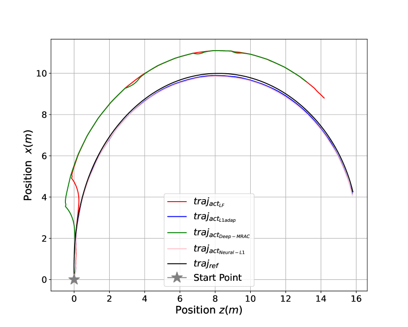
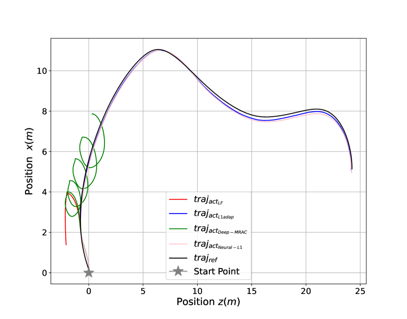
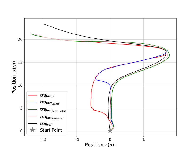
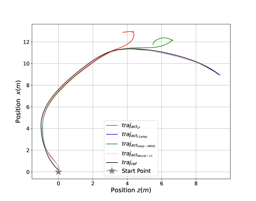
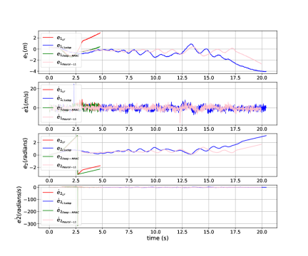
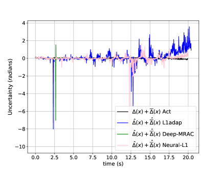
Trajectory tracking performance of all controllers, over arbitrary trajectories, is shown in Fig. 3. Over a circular reference (ref) trajectory in Fig. 3(a) with a constant radius and vehicle longitudinal velocity , Neural-L1 and L1adap exhibit a superior tracking performance in comparison to LF [1] and Deep-MRAC [18] controllers. Uncertainty, as plotted in black in Fig. 5, is introduced directly into the control law as a function of constant unknown parameters with added uniform white noise . Note that the constant unknown parameters and the uniform white noise add up to the total true uncertainty . In figures 3(b), 3(c) and 3(d) , we further provide the tracking performance results of all controllers over three other arbitrary trajectories with varying radius , even though the lateral error dynamics [4] is based on the assumption that the trajectory radius remains constant. Neural-L1 exhibits superior tracking performance in comparison to the other controllers as it successfully completes each of the four trajectories in figures 3(a), 3(b), 3(c) and 3(d) , whereas LF, L1adap and Deep-MRAC controllers fail to track at least one of the four ref trajectories.
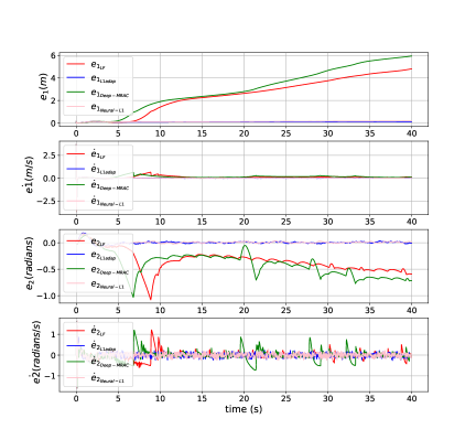
Next, in figures 4 and 5, we study the profiles of the states of the lateral error dynamics from [4] and the learned uncertainty of the adaptive controllers, only corresponding to the circular trajectory shown in Fig. 3(a). Thus, in Fig. 4, the states lateral error and yaw angle error deviate from the reference for LF controller and the Deep-MRAC controller, implying unstable behavior of the controllers. Only for the controllers Neural-L1 and L1adap all four states converge close to zero. This implies that both Neural-L1 and L1adap exhibit stability in the presence of disturbance directly induced into the control signal which is also the steering angle command in radians.
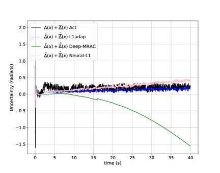
It is clear from the green plot in Fig. 5 that Deep-MRAC controller doesn’t learn the true uncertainty represented in black, whereas controllers L1adap, Neural-L1 are able to successfully learn the true uncertainty. This is because L1adap and Neural-L1controllers are robust in nature due to the selection of an appropriate strictly proper low pass filter , such that the -norm condition given in (12) is satisfied, enabling the controllers to attenuate the noise in the induced uncertainty.
VI Real Experiments
In this section we discuss the experimental setup and provide experimental results by evaluating our controller on the F1TENTH platform. We evaluate our proposed Neural-L1 against the LF, L1adap and the Deep-MRAC [18] controllers.
VI-A Experimental Setup
The control algorithms are deployed on an F1TENTH autonomous vehicle [49] running Jetson Xavier NX for onboard computation. For 6-DoF real-world state estimation, PhaseSpace X2E LED motion capture markers were attached to the autonomous vehicle which provide pose information at . ROS2 was used as the middleware stack for interfacing between sensors, autonomous agent and control algorithms [50]. For the F1TENTH, we test all the controllers with longitudinal velocities and . The F1TENTH is then made to track a circular trajectory with a constant radius and with added obstacles like a ramp at , and two wooden planks. The physical obstacles induce disturbance externally, in addition to induced sensor noise and control signal disturbance. In this regard, similar to the PyBullet simulation setup described in Section V, disturbance is directly injected into the control signal as constant unknown parameters with added uniform white noise . In addition, we also add uniform white noise to the PhaseSpace sensor pose readings. Note that the constant unknown parameters and the uniform white noise added to the control signal and the uniform white noise added to PhaseSpace sensor pose readings, add up to the total true uncertainty . The complete experimental setup is shown in Fig. 6.
VI-B Experimental Results
In this subsection, we discuss in detail the results from the real-world experiments conducted using the front-steered Ackermann vehicle F1TENTH. Fig. 7(a) shows the trajectory tracking performances of all the controllers at , with sensor noise and control signal disturbance, but without any physical obstacles. Fig. 7(b) shows the trajectory tracking performances of the controllers with ramp and planks added to the reference trajectory. The vehicle longitudinal velocity is increased to . The location of the physical obstacles, one ramp and two planks, are indicated in Fig. 7(b). As shown in figures 7(a) and 7(b), for both experiments, Neural-L1 tracks the trajectory exceptionally well and completes one loop of the circular trajectory, whereas LF, L1adap and Deep-MRAC controllers are not able to even complete one loop of the trajectory. Next, in figures 8 and 9, we study the profiles of the states, , of the lateral error dynamics from [4] and the learned uncertainty of the adaptive controllers corresponding to the circular trajectory shown in Fig. 7(b). In Fig. 8, the states lateral error and yaw angle error deviate from the reference for LF controller and the Deep-MRAC controller, implying unstable behavior of the controllers. Only for controllers Neural-L1 and L1adap, all four states remain in proximity to zero. Further, when the tracking error profiles of Neural-L1 and L1adap are compared in Fig 8, the errors and converge better for Neural-L1. This observation is not surprising because Neural-L1 controller is inherently based on the theory of L1adap. However, ultimately L1adap controller becomes unstable leading the F1TENTH vehicle to deviate from the ref trajectory. The deviation of the F1TENTH vehicle, due to the unstable behavior of L1adap controller, from the ref trajectory is clearly indicated by the increase in the magnitude of the state profiles and plotted in blue in Fig. 8 after .
These results can be better understood by studying the learned uncertainty profiles in Fig. 9. From Fig. 9, we notice that the uncertainty learned by Neural-L1 converges close to the true uncertainty , and the uncertainty learned by L1adap deviates at the end of the experiment. This is due to the external obstacles like ramp and planks added to the trajectory. These results imply that even though both L1adap and Neural-L1 controllers are robust in nature, the neural network is able to learn the uncertainties induced into the system by the presence of physical obstacles such as the ramp and the two planks, giving the Neural-L1 controller a better capability than the L1adap to learn the overall uncertainty. The oscillations induced in the trajectory, blue plot in Fig. 7(b), of the L1adap controller, right after the F1TENTH travels past plank 2, corroborate the observation in Fig. 9 that the learned uncertainty does not match the true uncertainty for L1adap. These oscillations lead the F1TENTH vehicle to not even complete one loop of the circular ref trajectory.
The increase in oscillations in the trajectory is further corroborated in and plots in Fig. 8, after about . Clearly, Neural-L1 controller handles these oscillations much better in comparison to L1adap controller, by keeping the errors close to zero. These results conclude that the Neural-L1 controller is stable as well as robust to disturbance and noises induced externally to the system, even when the disturbances are in the form of physical objects. For more extensive experimental results, we refer the reader to the video submission, where the superior tracking performance of the Neural-L1 controller is further exhibited by testing the Neural-L1 controllers over longer duration runs, with F1TENTH running over multiple loops of the circular ref trajectory. Our project page, including supplementary material and videos, can be found at https://mukhe027.github.io/Neural-Adaptive-Control/
VII Conclusions
In this paper, we addressed the problem of stable and robust control of front-steered Ackermann vehicles with lateral error dynamics for the application of lane keeping. We demonstrated that, in the presence of uncertainties induced into the control system, most existing controllers such as linear state-feedback controller (i.e. PID), Adaptive controller [1] and the Deep-MRAC [18] fail to track a reference trajectory. This is particularly due to the controllers’ inabilities to attenuate noise. Out of the three existing controllers, linear state-feedback controller, Adaptive controller [1] and the Deep-MRAC [18], Adaptive controller [1] exhibits the best tracking performance because unlike other controllers, Adaptive controller[1] is designed traditionally to be stable, adaptive as well as robust. However, under the circumstance of uncertainties that are induced as sensor noise, control signal disturbance and physical obstacles on the reference trajectory, even Adaptive controller [1] fails. Therefore, taking inspiration from the stability, adaptiveness and the robustness properties of the Adaptive controller [1] and combining it with the novel neural network approach of learning the adaptive laws in Deep-MRAC [18], we introduced the Neural Adaptive controller.
We demonstrated the effectiveness of the Neural Adaptive controller by taking a multi-tiered approach: i) We extended the theory of guaranteed stability, adaptiveness and robustness of Adaptive controller [1], while combining it with the neural network approach of Deep-MRAC [18], to the Neural Adaptive controller; ii) We conducted extensive physics-based simulation on PyBullet using a model of F1TENTH vehicle and compared the trajectory tracking performance of our proposed controller with the performance of other existing controllers; iii) We conducted real experiments using a F1TENTH platform and evaluated the performance of our controller. These results allowed us to conclude that the Neural adaptive controller behaves in a stable and robust manner in the presence of uncertainties induced into the dynamics and has superior tracking performance than a traditional linear state-feedback [4], the Deep-MRAC controller introduced in [18], and the conventional adaptive controller [1]. Future work could extend to use perception to learn features from the environment which in turn could be used to learn the true uncertainty more accurately and expand the stability results when the robots have noise from multiple sensors.
References
- [1] N. Hovakimyan, C. Cao, E. Kharisov, E. Xargay, and I. M. Gregory, “L 1 adaptive control for safety-critical systems,” IEEE Control Systems Magazine, vol. 31, no. 5, pp. 54–104, 2011.
- [2] A. Annaswamy, E. Lavretsky, Z. Dydek, T. Gibson, and M. Matsutani, “Recent results in robust adaptive flight control systems,” International Journal of Adaptive Control and Signal Processing, vol. 27, no. 1-2, pp. 4–21, 2013.
- [3] K. A. Wise, E. Lavretsky, and N. Hovakimyan, “Adaptive control of flight: theory, applications, and open problems,” in 2006 American Control Conference. IEEE, 2006, pp. 6–pp.
- [4] R. Rajamani, Vehicle dynamics and control. Springer Science & Business Media, 2011.
- [5] FHWA, “Roadway departure safety,” 2023.
- [6] D. Bevly, X. Cao, M. Gordon, G. Ozbilgin, D. Kari, B. Nelson, J. Woodruff, M. Barth, C. Murray, A. Kurt, et al., “Lane change and merge maneuvers for connected and automated vehicles: A survey,” IEEE Transactions on Intelligent Vehicles, vol. 1, no. 1, pp. 105–120, 2016.
- [7] R. Hindman, C. Cao, and N. Hovakimyan, “Designing a high performance, stable l1 adaptive output feedback controller,” in AIAA Guidance, Navigation and Control Conference and Exhibit, 2007, p. 6644.
- [8] C. Cao and N. Hovakimyan, “Adaptive controller for systems with unknown time-varying parameters and disturbances in the presence of non-zero trajectory initialization error,” International Journal of Control, vol. 81, no. 7, pp. 1147–1161, 2008.
- [9] ——, “Design and analysis of a novel l1 adaptive control architecture with guaranteed transient performance,” IEEE Transactions on Automatic Control, vol. 53, no. 2, pp. 586–591, 2008.
- [10] J. Wang, C. Cao, N. Hovakimyan, R. Hindman, and D. B. Ridgely, “L1 adaptive controller for a missile longitudinal autopilot design,” in AIAA Guidance, Navigation and Control Conference and Exhibit, 2008, p. 6282.
- [11] J. Wang, N. Hovakimyan, and C. Cao, “L1 adaptive augmentation of gain-scheduled controller for racetrack maneuver in aerial refueling,” in AIAA guidance, navigation, and control conference, 2009, p. 5739.
- [12] T. Leman, E. Xargay, G. Dullerud, N. Hovakimyan, and T. Wendel, “L1 adaptive control augmentation system for the x-48b aircraft,” in AIAA guidance, navigation, and control conference, 2009, p. 5619.
- [13] C. Cao and N. Hovakimyan, “L 1 adaptive output feedback controller for non strictly positive real multi-input multi-output systems in the presence of unknown nonlinearities,” in 2009 American Control Conference. IEEE, 2009, pp. 5138–5143.
- [14] P. A. Ioannou and J. Sun, Robust adaptive control. PTR Prentice-Hall Upper Saddle River, NJ, 1996, vol. 1.
- [15] K. S. Narendra and A. M. Annaswamy, Stable adaptive systems. Courier Corporation, 2012.
- [16] A. M. Annaswamy and S. Karason, “Discrete-time adaptive control in the presence of input constraints,” Automatica, vol. 31, no. 10, pp. 1421–1431, 1995.
- [17] J.-J. E. Slotine, “Applied nonlinear control,” PRENTICE-HALL google schola, vol. 2, pp. 1123–1131, 1991.
- [18] G. Joshi and G. Chowdhary, “Deep model reference adaptive control,” in 2019 IEEE 58th Conference on Decision and Control (CDC). IEEE, 2019, pp. 4601–4608.
- [19] H. Peng and D. Eisele, “Vehicle dynamics control with rollover prevention for articulated heavy trucks,” in Proceedings of 5th International Symposium on Advanced Vehicle Control, University of Michigan, Ann Arbor. Michigan USA, 2000.
- [20] J. Gohl, R. Rajamani, L. Alexander, and P. Starr, “The development of tilt-controlled narrow ground vehicles,” in Proceedings of the 2002 American Control Conference (IEEE Cat. No. CH37301), vol. 3. IEEE, 2002, pp. 2540–2545.
- [21] S. Kidane, L. Alexander, R. Rajamani, P. Starr, and M. Donath, “Control system design for full range operation of a narrow commuter vehicle,” in ASME International Mechanical Engineering Congress and Exposition, vol. 42169, 2005, pp. 473–482.
- [22] A. Lewis and M. El-Gindy, “Sliding mode control for rollover prevention of heavy vehicles based on lateral acceleration,” International Journal of Heavy Vehicle Systems, vol. 10, no. 1-2, pp. 9–34, 2003.
- [23] R. Rajamani and C. Zhu, “Semi-autonomous adaptive cruise control systems,” IEEE Transactions on Vehicular Technology, vol. 51, no. 5, pp. 1186–1192, 2002.
- [24] R. Rajamani, C. Zhu, and L. Alexander, “Lateral control of a backward driven front-steering vehicle,” Control Engineering Practice, vol. 11, no. 5, pp. 531–540, 2003.
- [25] C. J. Taylor, J. Košecká, R. Blasi, and J. Malik, “A comparative study of vision-based lateral control strategies for autonomous highway driving,” The International Journal of Robotics Research, vol. 18, no. 5, pp. 442–453, 1999.
- [26] D. Wang and F. Qi, “Trajectory planning for a four-wheel-steering vehicle,” in Proceedings 2001 ICRA. IEEE International Conference on Robotics and Automation (Cat. No. 01CH37164), vol. 4. IEEE, 2001, pp. 3320–3325.
- [27] C. Thorpe, M. Hebert, T. Kanade, and S. Shafer, “Vision and navigation for the carnegie-mellon navlab,” Annual Review of Computer Science, vol. 2, no. 1, pp. 521–556, 1987.
- [28] H. Mouri and H. Furusho, “Automatic path tracking using linear quadratic control theory,” in Proceedings of Conference on Intelligent Transportation Systems. IEEE, 1997, pp. 948–953.
- [29] M. Akar and J. C. Kalkkuhl, “Lateral dynamics emulation via a four-wheel steering vehicle,” Vehicle System Dynamics, vol. 46, no. 9, pp. 803–829, 2008.
- [30] J. E. Naranjo, C. Gonzalez, R. Garcia, and T. De Pedro, “Lane-change fuzzy control in autonomous vehicles for the overtaking maneuver,” IEEE Transactions on Intelligent Transportation Systems, vol. 9, no. 3, pp. 438–450, 2008.
- [31] L. Cai, A. B. Rad, W.-L. Chan, and K.-Y. Cai, “A robust fuzzy pd controller for automatic steering control of autonomous vehicles,” in The 12th IEEE International Conference on Fuzzy Systems, 2003. FUZZ’03., vol. 1. IEEE, 2003, pp. 549–554.
- [32] T. Keviczky, P. Falcone, F. Borrelli, J. Asgari, and D. Hrovat, “Predictive control approach to autonomous vehicle steering,” in 2006 American control conference. IEEE, 2006, pp. 6–pp.
- [33] P. Falcone, F. Borrelli, J. Asgari, H. E. Tseng, and D. Hrovat, “Predictive active steering control for autonomous vehicle systems,” IEEE Transactions on control systems technology, vol. 15, no. 3, pp. 566–580, 2007.
- [34] J.-H. Lee and W.-S. Yoo, “An improved model-based predictive control of vehicle trajectory by using nonlinear function,” Journal of mechanical science and technology, vol. 23, pp. 918–922, 2009.
- [35] R. Marino, S. Scalzi, G. Orlando, and M. Netto, “A nested pid steering control for lane keeping in vision based autonomous vehicles,” in 2009 American Control Conference. IEEE, 2009, pp. 2885–2890.
- [36] H. Zang and M. Liu, “Fuzzy neural network pid control for electric power steering system,” in 2007 IEEE International Conference on Automation and Logistics. IEEE, 2007, pp. 643–648.
- [37] A. Haytham, Y. Z. Elhalwagy, A. Wassal, and N. Darwish, “Modeling and simulation of four-wheel steering unmanned ground vehicles using a pid controller,” in 2014 international conference on engineering and technology (ICET). IEEE, 2014, pp. 1–8.
- [38] P. Hammer, “Adaptive control processes: a guided tour (r. bellman),” 1962.
- [39] A. Zinober, “Adaptive control: the model reference approach,” Electronics and Power, vol. 26, no. 3, p. 263, 1980.
- [40] A. Morse, “Global stability of parameter-adaptive control systems,” in 1979 18th IEEE Conference on Decision and Control including the Symposium on Adaptive Processes, vol. 2. IEEE, 1979, pp. 1041–1045.
- [41] C. E. Rohrs, “Adaptive control in the presence of unmodeled dynamics,” Tech. Rep., 1982.
- [42] W. Morse and K. Ossman, “Flight control reconfiguration using model reference adaptive control,” in 1989 American Control Conference. IEEE, 1989, pp. 159–164.
- [43] Z. Wu, S. Cheng, K. A. Ackerman, A. Gahlawat, A. Lakshmanan, P. Zhao, and N. Hovakimyan, “L 1 adaptive augmentation for geometric tracking control of quadrotors,” in 2022 International Conference on Robotics and Automation (ICRA). IEEE, 2022, pp. 1329–1336.
- [44] K. Huang, R. Rana, A. Spitzer, G. Shi, and B. Boots, “Datt: Deep adaptive trajectory tracking for quadrotor control,” arXiv preprint arXiv:2310.09053, 2023.
- [45] M. M. Shirazi and A. B. Rad, “ adaptive control of vehicle lateral dynamics,” IEEE Transactions on Intelligent Vehicles, vol. 3, no. 1, pp. 92–101, 2017.
- [46] B. M. Gonultas, P. Mukherjee, O. G. Poyrazoglu, and V. Isler, “System identification and control of front-steered ackermann vehicles through differentiable physics,” in 2023 IEEE/RSJ International Conference on Intelligent Robots and Systems (IROS). IEEE, 2023, pp. 4347–4353.
- [47] E. Coumans and Y. Bai, “Pybullet, a python module for physics simulation for games, robotics and machine learning,” http://pybullet.org, 2016–2021.
- [48] V. S. Babu and M. Behl, “f1tenth. dev-an open-source ros based f1/10 autonomous racing simulator,” in 2020 IEEE 16th International Conference on Automation Science and Engineering (CASE). IEEE, 2020, pp. 1614–1620.
- [49] M. O’Kelly, H. Zheng, D. Karthik, and R. Mangharam, “F1tenth: An open-source evaluation environment for continuous control and reinforcement learning,” Proceedings of Machine Learning Research, vol. 123, 2020.
- [50] S. Macenski, T. Foote, B. Gerkey, C. Lalancette, and W. Woodall, “Robot operating system 2: Design, architecture, and uses in the wild,” Science robotics, vol. 7, no. 66, p. eabm6074, 2022.
![[Uncaptioned image]](/html/2405.16358/assets/fig/bio/pratik.jpg) |
Pratik Mukherjee received his B.S. and M.S. degree in mechanical engineering from University of Minnesota Twin-Cities, Minneapolis, USA, in 2014 and 2016, respectively. He obtained his Ph.D. degree in electrical engineering from Virginia Tech, Blacksburg, VA, USA, as part of the Coordination at Scale Laboratory. He is currently working as Postdoctoral Associate at the University of Minnesota Twin-Cities, Minneapolis, USA in the computer science department in the Robotic Sensor Networks Lab. His current research interests include distributed, stable and robust topology control applied to single or multi-robot systems. He is an incoming Assistant Professor at Florida Atlantic University, Boca Raton, FLorida in the Ocean and Mechanical Engineering Department. |
![[Uncaptioned image]](/html/2405.16358/assets/fig/bio/burak.jpeg) |
Burak M. Gonultas received his B.S. degrees in electronics and communication engineering and computer engineering from Istanbul Technical University, Istanbul, Turkey, in 2018 and 2019, respectively. As a Ph.D. candidate he is currently working as Research Assistant at the University of Minnesota Twin-Cities, Minneapolis, USA in the computer science department in the Robotic Sensor Networks Lab. His current research interests include planning, dynamics, control and multi-agent reinforcement learning for autonomous mobile systems. |
![[Uncaptioned image]](/html/2405.16358/assets/fig/bio/goktug.jpeg) |
O. Goktug Poyrazoglu received his B.S. degree in mechanical engineering from Bilkent University, Ankara, Turkey, in 2020. He is currently working as Ph.D. Student at the University of Minnesota Twin-Cities, Minneapolis, USA in the computer science department in the Robotic Sensor Networks Lab. His current research interests include trajectory optimization, quantifying uncertainty, and modeling environmental interactions for mobile robotic applications. |
![[Uncaptioned image]](/html/2405.16358/assets/fig/bio/volkan.jpg) |
Volkan Isler received the B.S. degree in computer engineering from Bogazici University, Istanbul, Turkey, in 1999, and the M.S.E. and Ph.D. degrees in computer and information science from University of Pennsylvania, Philadelphia, PA, USA, in 2000 and 2004, respectively. He is currently a Professor in the Department of Computer Science & Engineering with University of Minnesota, Minneapolis, MN, USA where he directs the Robotic Sensor Networks Lab. From 2020 to 2023, he was the head of Samsung’s AI Center in NY. His research interests include geometric algorithms for perception and planning, and their applications to agricultural and consumer robots. From 2009 to 2015, he was the Chair of the Robotics and Automation Society Technical Committee on networked robots. He received the CAREER Award from the National Science Foundation, and McKnight Land-grant professorship from the University of Minnesota. |