Prudent Price-Responsive Demands

Abstract

We investigate a flexible demand with a risk-neutral cost-saving objective in response to volatile electricity prices. We introduce the concept of prudent demand, which states that future price uncertainties will affect immediate consumption patterns, despite the price expectations remaining unchanged. We develop a theoretical framework and prove that demand exhibits prudence when the third-order derivative of its utility cost function is positive, and show a prudent demand demonstrates risk-averse behaviors despite the objective being risk-neutral. Our analysis further reveals that, for a prudent demand, predictions of future price skewness significantly impact immediate energy consumption. Prudent demands exhibit skewness aversion, with increased price skewness elevating the cost associated with prudence. We validate our theoretical findings through numerical simulations and conclude their implications for demand response modeling and the future design of incentive-based demand response mechanisms.

Keywords: OR in energy, Demand response, Prudence, Risk behavioral, Sequential decision-making,

1 Introduction

Utility and load-serving entities are introducing dynamic pricing models to promote flexible demand solutions, including storage units, smart appliances, and electric vehicles [Saad et al., 2016], expecting consumers to strategically adjust their electricity usage to minimize costs. This is also a promising way to realize efficient, fair, and equitable tariffs [Borenstein, 2016, Burger et al., 2019]. In the example of real-time pricing schemes, electricity prices fluctuate over time and are disclosed only at the point of delivery [Chen et al., 2012, Ameren, nd]. Such price variability, influenced by wholesale market rates or local grid conditions, delivers incentive-based demand response (DR) [Liu et al., 2017] at a relatively low cost to improve reliability [Qdr, 2006] and reduce the demand during system contingencies [Deng et al., 2015].

While real-time tariffs grant utilities the flexibility to modify prices in response to current conditions, they also introduce a layer of uncertainty for consumers. Introducing consumers to fluctuating electricity prices elicits complex risk-aware behaviors [Wei et al., 2014], which must be studied systematically for efficient and equitable tariff design [Khan et al., 2023]. To this end, due to the complexity of conducting real-world tariff experiments associated with infrastructure constraints and privacy concerns, it is more practical to adopt decision-making models. A critical aspect of these models is selecting a utility function that accurately represents the costs and constraints encountered during response events. Previous literature has used quadratic or piece-wise linear utility functions inspired by the operational characteristics of household appliances, thermal comfort considerations, and battery storage capabilities [Li et al., 2011, Jia and Tong, 2016, Zheng et al., 2022].

Nevertheless, the simplicity of quadratic or linear utility functions often fails to accurately capture consumers’ nuanced preferences and constraints. For example, thermal comfort does not decrease linearly with temperature adjustments or change in a purely quadratic manner. Instead, it is influenced by individual, high-dimensional, non-linear preferences [Tang and Wang, 2019, Vázquez-Canteli and Nagy, 2019]. Similarly, batteries and many household appliances operate within strict capacity and ramp rate limits that a quadratic model, with its inherent soft penalties, inadequately represents. On the other hand, model-free learning methods have begun to explore such advanced formulations [Antonopoulos et al., 2021], but the application is limited to the scarce data availability in this domain.

Prior studies underscore the need for a more sophisticated utility function formulation. Motivated by a classical economic concept called prudence, which reflects the sensitivity of the optimal response to risk [Kimball, 1989, Peter, 2017], i.e., how demands are prepared to respond to various future risks with the same expectations [Menegatti, 2014]. The detailed contributions are as follows:

• We establish a theoretical framework to model demand behavior to future volatile electricity prices with a constant expectation value. The demand is modeled with a risk-neutral cost-saving objective in a sequential non-anticipatory decision-making context.

• We found that demand models with quadratic utility/cost functions are distribution-insensitive, i.e., if the expectation of the price is unchanged, then the demand will not change its action prior to the price events based on the associated uncertainties.

• We prove that super-quadratic cost functions (higher order than two) result in prudent demands. Specifically, prudent demand exhibits aversion to price distribution skewness (also known as asymmetric), in which the demand will change its consumption before the price event if the price distribution is skewed, and this change of consumption increases with the skewness.

• We use simulation to verify our results with regard to distribution-insensitive and prudent demand models and show their implications for future dynamic tariff mechanism designs.

The remaining of the paper is organized as follows: Section II reviews related literature, Section III introduces the distribution-insensitive demands’ definition and conditions, Section IV extends to prudent demands’ analysis in terms of definition, conditions, and revelation, Section V describes simulation results under DR settings, and Section VI concludes the paper.

2 Background and literature review

2.1 Dynamic pricing for residential consumers

Dynamic pricing schemes, also known as the time-varying price, are designed to utilize demand-side flexibility but also introduce variability to the electricity prices [Borenstein, 2016, Burger et al., 2019]. Electricity prices at wholesale markets are inherently variable [Ercot, nd], and in regions like Texas, consumers can elect to receive wholesale real-time prices directly. During the 2021 winter storm Uri, the wholesale real-time price surged to $9,000/MWh in Texas [Douglas and Foxhall, 2023], and some families consumers received outrageous electricity bills of more than ten thousand as they still kept lights and heat on [Giulia et al., 2021].

On the retailer side, utilities are adopting dynamic tariffs to incentivize demand responses. There are many utility issues with time of use (ToU) tariffs for residential customers with peak and off-peak rates to provide consumers with the greatest opportunity for savings, such as Con Edison in New York City [ConEd, nd], PG&E in California [PG&E, nd], and Salt River Project in Arizona [SRP, nd]. Beyond ToU, utilities are now experimenting with more advanced time-varying tariffs. For example, OG&E in Oklahoma uses a smart hour pricing scheme that varies prices during ToU peak hours [OG&E, nd]; Ameren in Illinois uses a power smart pricing rate plan that issues hourly different electricity prices to residential customers day ahead [Ameren, nd]. All these plans indicate the need to use dynamic pricing to incentivize improved consumer flexibility.

2.2 Incentive-based demand response

The key to dynamic tariff design is to understand how consumers would respond. However, concerns about privacy, affordability, and fairness make it difficult to conduct controlled real-world experiments, especially with variable real-time tariffs. Instead, plenty of prior research has explored using model-based approaches to use speculative utility functions to represent consumers’ decision-making processes [Mohsenian-Rad et al., 2010], such as shifting appliance usages or thermal discomforts [Samadi et al., 2010, Li et al., 2017].

Quadratic functions are widely used to represent utility function [Jordehi, 2019]. The reason is that the optimal solution of the utility maximization problem comes from the first-order optimality condition, which requires a concave and monotonic increase function [Chen et al., 2012, Deng et al., 2015]. The classical representation is the quadratic type, which can also keep a reasonable computation performance and even obtain the closed-form solution [Jia and Tong, 2016]. However, the quadratic function gives compromises to elegant math analysis [Morales-España et al., 2022], which may not reflect the real customer’s response performance. On the other hand, learning methods learn customers’ consumption patterns expressed as the utility function parameters [Kwac and Rajagopal, 2015, Li et al., 2017, Mieth and Dvorkin, 2019], integrate user’ feedback into the control loop [Vázquez-Canteli and Nagy, 2019], and even reflect individual’s response behavior through model-free formulation [Antonopoulos et al., 2021]. Still, these methods face the risk of extrapolating consumer behavior to new price patterns.

Consumers’ responses to uncertain prices are even less understood in literature due to the scarcity of data availability. While one would expect consumers will demonstrate risk-averse behaviors when imposed with volatile prices, studies on this topic introduce artificial risk-aversion constraints, such as robust [Wei et al., 2014] or conditional value-at-risk (CVaR) [Roveto et al., 2020, Jia and Tong, 2012], but lack of first-principle understanding of risk-aversion motivations. In summary, like the quadratic consideration, these risk preferences are exogenous to the agent’s behavior model and are added intentionally. More natural demand response behavior still needs to be studied to determine how the agent will respond to the price.

2.3 Theory of prudence

Prudence means seeing ahead and sagacity, a classical economic concept that expresses the sensitivity of the optimal response to risk [Kimball, 1989]. Originated from but different from the risk aversion behavior first defined by Pratt, which indicates that risk aversion is an attitude to risk and shows how people dislike risk but without response [Pratt, 1978]. Kimball first introduces prudence from a precautionary saving perspective, which is how much one could save by preparing responses to risk ahead of time [Kimball, 1989]. By definition, risk aversion is determined by the second-order derivative of the agent’s utility function, which is a lower-order risk attitude and can be implied by a higher-order risk attitude, such as third-order prudence or fourth-order temperate [Menegatti, 2014]. As the risk attitude moves to a higher order, the formulation can reflect consumers’ effort level change to prepare the response to the risk [Peter, 2017].

As describing the risk preference more than an attitude, prudence is proved to imply inherent risk aversion behavior and make a loss-averse decision maker [Eeckhoudt et al., 2016]. From a theoretical perspective, the prudent consumer is proven to make more effort ahead of time to expect a larger wealth in the risk period [Menegatti, 2009], even in the presence of deeper uncertainty, i.e., ambiguity, that the risk distribution is unknown [Berger, 2016]. Prudence has also been proven to be related to skewness preference. Consumers generally bear a higher level of overall risk or lower payoff with right-skewed risk, which naturally motivates the left-skewed seeking behavior [Eeckhoudt and Schlesinger, 2006]. This behavior is then proved to align with prudence that prefers to apportion risk [Ebert and Wiesen, 2014]. Empirical evidence has also been found and shown in experiments regarding prudence and risk-averse behavior [Mayrhofer and Schmitz, 2020] and prudence and skewness correlations [Ebert and Wiesen, 2011].

All these behaviors are finally reflected in optimal decision-making under uncertainty. When only considering the risk happens time, prudence with higher-order properties reflects more than risk aversion by measuring the discount factors change due to the variant outcomes time [Ebert, 2020]. Prudence also shows knowing less means doing more [Li and Peter, 2021], which makes them more accepting of the cost of any risk management methods under unforeseen future [Reichel et al., 2021]. That is because consumers can compensate and lower exposure to risk by using those risk management methods, generally reflected as preparing their effort ahead of time [Menegatti, 2015]. Although many studies show optimal decision-making under uncertainty cases, the application and influence of prudent behavior on electricity customers’ price response behavior haven’t been studied yet, especially in a multi-period sequential decision-making framework.

3 Model and Preliminaries

In this section, we formulate our model and introduce the definitions. We consider demand with a risk-neutral cost-saving objective and linear system model responding to future electricity price uncertainty in a discrete time-varying system with stage $t\in[1,T]$. The objective is to minimize the expectation of all stages’ costs,

$$\min_{p_{t}} \;\mathbb{E}_{\Lambda_{t}}\sum_{t=1}^{T}\Big{[}\lambda_{t}p_{t}+C_{t}(x_{t})+G_{t}(p_{t})\Big{]}+V_{T}(x_{T}),$$ (1a)

s.t. $$x_{t}=Ax_{t-1}+p_{t},$$ (1b)

$$p_{t}$$ is non-anticipatory (1c)

where $\lambda_{t}$ is the uncertain price at stage $t$ come from a distribution $\Lambda_{t}$, $\Lambda_{t}\in\mathcal{L}_{t}$. $p_{t},x_{t}$ are the power action and states at stage $t$, respectively; the state value can represent factors such as battery state-of-charge (SOC) or temperature. $C_{t}(x_{t}),G_{t}(p_{t})$ are the state and action cost functions, respectively. $V_{T}(x_{T})$ is the end state-value function, representing the state value at the final stage for value continuity and can be set to zero to show no final value. (1b) is the state transition constraint with the state discount factor $A\leq 1$. Finally, (1c) states the control is non-anticipatory to reflect the nature of multi-stage stochastic decision-making [Shapiro et al., 2021].

Definition 1.

Normalized power and state cost. We apply unit normalization and assume the system is in equilibrium at zero power and state to simply the model and highlight our focus on disturbances and variations. For example, a Heating, Ventilation, and Air Conditioning (HVAC) system is set to control the room temperature to 25 Celsius, and then in our normalized system, the room temperature corresponds to $x_{t}=0$ and $C_{t}(0)=0$ represents no thermal discomforts. Formally, the normalization provides $C_{t}(0)=0$ and $G_{t}(0)=0$, with $C_{t}(x_{t})\geq 0$ and $G_{t}(p_{t})\geq 0$. We also define $G_{t}$ and $C_{t}$ are continuous and convex. Fig. 1 provides an example of the power and state cost functions.

Remark 2.

Modeling hard constraints. We can use the state cost function $C_{t}$ and action cost function $G_{t}$ to represent the hard and soft upper/lower bounds of states and actions. A lower-order model, such as quadratic functions, can represent soft constraints, allowing for reasonable violations with moderate penalties. On the other hand, higher-order functions, such as the log barrier function and exponential function, can be employed to express hard constraints, imposing substantial penalties on decision-makers for any violations.

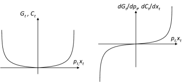
Figure 1: Graph of function $C_{t},G_{t}$ and their derivative.

Definition 3.

Quadratic and super quadratic function. We denote $a_{\mathrm{p}}$ as the function parameter and define the quadratic function as the following

$$G_{t}(p_{t})=\frac{a_{\mathrm{p}}p_{t}^{2}}{2},a_{\mathrm{p}}>0,$$ (2a)

We define a super quadratic function as a function whose third-order derivative is not zero,

$$\frac{\partial^{3}G_{t}(p_{t})}{\partial p_{t}^{3}}\neq 0.$$ (2b)

Stochastic dynamic programming reformulation. To reflect the non-anticipatively in the sequential decision-making under uncertainty, we use stochastic dynamic programming to reformulate (1) by working backward and recursively solving a single-stage optimization, i.e., $\forall t\in[1,T]$:

$$Q_{t-1}(x_{t-1}|\lambda_{t})= \min_{p_{t}}\lambda_{t}p_{t}+C_{t}(x_{t})+G_{t}(p_{t})+V_{t}(x_{t})$$ (3a)

$$V_{t}(x_{t})= \mathbb{E}_{\Lambda_{t+1}}[Q_{t}(x_{t}|\lambda_{t+1})]$$ (3b)

$$\text{s.t.}\ x_{t}= Ax_{t-1}+p_{t}.$$ (3c)

where $Q_{t-1}(x_{t-1}|\lambda_{t})$ is the action-value function at stage $t-1$ parameterized by the price $\lambda_{t}$ at stage $t$, and $V_{t}(x_{t})$ is the state-value function at stage $t$.

We show the notation used in the whole paper. We use $g_{t}(p_{t})=\partial G_{t}(p_{t})/\partial p_{t}$, $c_{t}(x_{t})=\partial C_{t}(x_{t})/\partial x_{t}$, $v_{t}(x_{t})=\partial V_{t}(x_{t})/\partial x_{t}$, $q_{t}(x_{t}|\lambda_{t+1})=\partial Q_{t}(x_{t}|\lambda_{t+1})/\partial x_{t}$ to express the first-order derivative of the action cost function, state cost function, state-value function, and action-value function, respectively, and above $\cdot$ to express second-order derivative, such as $\dot{g}$. We also combine the derivative of state-related cost and express it as $h_{t}(x_{t})$, i.e., $h_{t}(x_{t})=c_{t}(x_{t})+v_{t}(x_{t})$.

4 Distribution-insensitive demand models

In this section, we show the conditions for a demand model described in (3) to be distribution-insensitive: the demand only responds to changes in future price expectations but is insensitive to changes in the price distribution if the expectations remain the same. The following theorem formally introduces this characteristic.

Theorem 4.

Distribution-insensitive demand models. Consider the price $\lambda_{t}$ come from distribution $\Lambda_{t},\Gamma_{t}$, $\{\Lambda_{t},\Gamma_{t}\}\in\mathcal{L}_{t}$ at stage $t$ with a fixed expectation $\mathbb{E}_{\Lambda_{t}}[\lambda_{t}]=\mathbb{E}_{\Gamma_{t}}[\lambda_{t}]$. Then a demand model described in (3) with quadratic state cost function $C_{t}$ and action cost functions $G_{t}$ following Definitions 1 and 3 satisfies the distribution-insensitive conditions that consumption at stage $t$ will not be affected by the distributions at stage $t+1$, i.e.,

$$\mathbb{E}_{\Gamma_{t+1}}[Q_{t}(x_{t}|\lambda_{t+1})]=\mathbb{E}_{\Lambda_{t+1}}[Q_{t}(x_{t}|\lambda_{t+1})],\forall\{\Lambda_{t+1},\Gamma_{t+1}\}\in\mathcal{L}_{t+1}$$ (4)

Sketch of the proof.

To prove this theorem, we first show the current action-value function derivative equals to the future state-related cost derivatives, i.e., $q_{t}(x_{t}|\lambda_{t+1})=h_{t+1}(x_{t+1}(\lambda_{t+1}))$. Then, by taking the derivative of $h_{t+1}$ with regards to $\lambda_{t+1}$, we are able to analyze the relationship between the derivative of the action-value function $q_{t}(x_{t}|\lambda_{t+1})$ and future price $\lambda_{t+1}$. Then, we show state-value function derivative $v_{t}$ is a linear combination of all future function $c_{\tau},\tau\in[t+1,T]$, indicating, under the Theorem’s conditions, $h_{t+1}(x_{t+1}(\lambda_{t+1}))$ is a linear function with regard to $\lambda_{t+1}$, and thus we conclude the linear relationship between $q_{t}(x_{t}|\lambda_{t+1})$ and $\lambda_{t+1}$. We then prove the linear relationship between $q_{t}(x_{t}|\lambda_{t+1})$ and $\lambda_{t+1}$ is necessary and sufficient for the distribution-insensitive conditions and completes the proof of the Theorem.

The detailed proof is provided in the appendix. ∎

The theorem indicates the consumption decision of demand, with a quadratic action and state cost function, is independent of the future price distribution, but only the expectation. Specifically, given more variant future price uncertainty with the same expectation, distribution-insensitive demand decisions in the earlier stages remain the same. When state and action are within a reasonable range, price term $\lambda_{t}p_{t}$ dominates the objective function. Thus, from the objective function perspective, increasing price uncertainty or facing extreme prices do bring higher costs to the demands, but by the Theorem 4, demands do nothing to respond to the risk. This aligns with the lower-order risk analysis, i.e., risk-averse preference, that demands only show the risk attitude - like or dislike risk, instead of a response behavior [Kimball, 1989, Pratt, 1978]. This theorem rigorously shows the connection between stage $t$ and $t+1$, naturally motivating us to think about the relationship in a broader time horizon.

Corollary 5.

Stage extrapolation. Under the same conditions of Theorem 4, the distribution-insensitive demand model can be extrapolated to all future periods that the consumption at stage $t$ is independent of all future distributions with fixed expectations at stage $\tau$, $\tau\in[t+1,T]$.

Proof.

We prove this Corollary by deduction. From Theorem 4, consumption at stage $t$ is independent of the price distribution at stage $t+1$, and the independence also holds for consumption at stage $t+1$ and price distribution at stage $t+2$. Following the state transition process, the consumption at stage $t$ is independent of price distribution at stage $t+2$. Thus, recursively, consumption at stage $t$ is independent of all future price distributions. ∎

This Corollary indicates the distribution-insensitive conditions hold for the price uncertainty in all future periods with fixed expectations. Motivated by the distribution-insensitive conditions, we naturally provide distribution-sensitive analysis in the following Corollary.

Corollary 6.

Distribution-sensitive demand models. Consider the price distribution described in Theorem 4, given that either or both super quadratic state cost function $C_{t}$ and action cost function $G_{t}$ following Definitions 1 and 3, the demand model in (3) becomes distribution-sensitive, except an extra case that has symmetrical price distributions with a mean of zero and demand’s prior state is zero, i.e., $\mathbb{E}_{\Lambda_{t+1}}[\lambda_{t+1}]=0,x_{t-1}=0$.

Proof.

The proof is provided in the appendix. ∎

This Corollary indicates the conditions of the distribution-sensitive demand model. Note that the extra distribution-insensitive case is unrealistic as price distribution, in practice, is generally skewed with a mean of nonzero. Also, consumers generally show higher-order utility functions (higher than quadratic). For example, when the temperature gets extremely hot or cold, consumers’ thermal discomforts increase dramatically, and many devices, like batteries, have hard constraints regarding their capacity. These two points naturally cause a distribution-sensitive demand and challenge the quadratic distribution-insensitive demands, which highlights using super quadratic formulations to study the demands’ response behaviors under uncertain future conditions.

5 Prudent demand models

In this section, we introduce prudent demand, which means demand apportions risk across the stages, and the demand level changes ahead of time, affected by future price distributions and expectations [Eeckhoudt and Schlesinger, 2006]. We illustrate the connection between future price distribution $\Lambda_{t+1}$ and earlier stages’ demand level $p_{\tau},\tau\in[1,t]$ and show demand with super quadratic state cost $C_{t}$ and quadratic action cost $G_{t}$ exhibits prudence. We reveal the skewness aversion behavior of prudent demand, where price skewness causes higher demand levels in the earlier stages, and this change of demand levels increases with the skewness.

To show the prudent behavior of demand that is sensitive to future price distributions, we introduce special two-point price distributions as the base to build the framework to analyze other complicated distributions. Then, we introduce the main Theorem in this paper.

Theorem 7.

Prudent demand models.

Consider the price $$\lambda_{t} \Lambda_{t}(\gamma_{t},\pi_{t}) \Gamma_{t}(\gamma_{t},\pi^{\prime}_{t}) t w_{\Lambda_{t}},w_{\Gamma_{t}}\in[0,0.5]$$ come from two-point distributions , at stage satisfying the following given :

$$-\mathbb{E}[\lambda_{t}]<\gamma_{t}<\pi_{t} <\pi^{\prime}_{t},$$ (5a)

$$-(1-w_{\Lambda_{t}})\gamma_{t}+w_{\Lambda_{t}}\pi_{t} =\mathbb{E}_{\Lambda_{t}}[\lambda_{t}],$$ (5b)

$$-(1-w_{\Gamma_{t}})\gamma_{t}+w_{\Gamma_{t}}\pi^{\prime}_{t} =\mathbb{E}_{\Gamma_{t}}[\lambda_{t}],$$ (5c)

$$\mathbb{E}_{\Lambda_{t}}[\lambda_{t}]=\mathbb{E}_{\Gamma_{t}}[\lambda_{t}] =\mathbb{E}[\lambda_{t}]\geq 0.$$ (5d)

Then a demand model described in (3), with super quadratic state cost function $$C_{t} G_{t} x_{0}=0 \lambda_{\tau}=0,\tau\in[1,t] t t+1$$ and quadratic action cost function following Definitions 1 and 3, under the conditions of , , satisfy the prudence and its sensitivity conditions that demand’s consumption before stage shows the following properties with regard to price distributions at stage :

$$\mathbb{E}_{\Gamma_{\tau+1}}[Q_{\tau}(x_{\tau}|\lambda_{\tau+1})]\geq\mathbb{E}_{\Lambda_{\tau+1}}[Q_{\tau}(x_{\tau}|\lambda_{\tau+1})]\geq Q_{\tau}(x_{\tau}|\mathbb{E}_{\Lambda_{\tau+1}}[\lambda_{\tau+1}])\geq 0,\forall\tau\leq t$$ (5e)

Sketch of the proof.

This theorem shows future two-point price distribution with fixed expectations affects the current state-value function of the demand, and then affects demands’ actions in the earlier stages. Here, we study the right skewness condition, and distribution $\Gamma$ is more right skewness compared with distribution $\Lambda$, and the left skewness follows the same analysis, which we show in the remark. The overview of this proof is to find the causal relationship between future price distribution and prior actions, with connecting variables and functions, i.e., $\Lambda_{t+1}\sim q_{t}\sim v_{t}\sim x_{t}\sim p_{\tau,\forall\tau\in[1,t]}$. Specifically, we first connect future price distribution $\Lambda_{t+1}(\gamma_{t+1},\pi_{t+1})$ with the current state-value function derivative $v_{t}$ by the model definition. Then, we connect the state and action $x_{t},p_{t}$ to the future price $\gamma_{t+1},\pi_{t+1}$. This helps us rewrite the state-value function derivative $v_{t}$ as a function of future price. Then, we analyze the property of reverse state-value function derivative $-v_{t}$, and include $\Gamma_{t+1}$ distributions to show the sensitivity of prudent demand. The proof consists of four general steps:

• We first assume $V_{t+1}(x_{t+1})=0$ and write out the optimality conditions for demands’ actions [Boyd and Vandenberghe, 2004]. Then, we show the state-value function derivative $v_{t}$ in the optimality conditions can be written as a function of future price;

• From the optimality conditions of actions (states) at stage $t+1$, we reveal the function relationship between price $\gamma_{t+1},\pi_{t+1}$ and state $x_{t+1}$, and show its monotonicity, symmetry, and concavity.

• By using the price and state function property from the last step, we show the reverse state-value function derivative $-v_{t}$ in the optimality conditions is positive and greater when using price distributions than when using price expectations, and the state value $x_{t}$ follows.

• To analyze the optimality conditions with more right skewness price distribution $\Gamma_{t+1}$, we further prove the sensitivity of the reverse state-value function derivative $-v_{t}$. We show a strict increase in $x_{t}$ with the right price skewness. Combined with the objective function and state transition, we show all earlier stages’ states and actions should be non-negative and non-decrease with the skewness and complete the proof of Theorem 7.

The full version of the proof is provided in the appendix. ∎

Remark 8.

Mirror theorem for left skewness. From the Theorem 7, demands show prudence with right skewness price distributions $\Lambda,\Gamma$. As the system is linear and the cost function is symmetrical, the prudence and its sensitivity conditions also stand for left skewed price distribution $\Gamma_{\mathrm{l}}(\gamma^{\prime},\pi)$ and $\Lambda(\gamma,\pi)$ from Theorem 7, i.e., $-\mathbb{E}[\lambda]<\gamma^{\prime}<\gamma<\pi$, $-(1-w_{\mathrm{l}})\gamma^{\prime}+w_{\mathrm{l}}\pi=\mathbb{E}[\lambda]\geq 0,w_{\Lambda},w_{\mathrm{l}}\in[0.5,1]$.

This theorem implies the conditions for the demand model, with higher-order formulations, to be prudent. These results also align with the definition of prudence in economics, specifically within expected utility theory, first introduced by Kimball [Kimball, 1989], requiring the positive third-order derivative of the utility function. We prove this in our case by showing the state value $x_{t}>0$, and the state-value function derivative $v_{t}$ is convex regarding $x_{t}$ when $x_{t}>0$.

To be specific, notify consumers of an event with skewed price uncertainty in a future stage $t+1$; demand shows prudence that the action (demand) level during all prior periods changes, either increasing or keeping the same. Note that the demand level changes are affected by both price expectation and distribution, i.e., applying distribution causes more change than using expectation value. This pre-preparation performance reflects the inherent skewness-averse (risk-averse) response behavior of demand, instead of only bearing more cost. Also, more skewness causes higher demand levels ahead of time, i.e., considering more skewed price distributions $\Gamma_{\mathrm{l}}$ with the same expectation, the state value $x_{t}$ strictly increases with the skewness of the price distribution. In practice, this theorem indicates we may obtain unexpected results when designing events. For example, the utility company may notify the consumers of a demand response event ahead of time and expect the consumer to shift their demand away from the peak time, but the demand shows prudence that will be prepared for the event ahead of time, which may cause another demand peak.

Note that we only imply the decision behavior before the event, i.e., $[1,t]$. We directly show the increase of the reverse state-value function derivative and the state value just ahead of the event (stage $t$). From the cost functions and state transition process, we obtain actions and states in earlier stages. We show that the state value increment at stage $t$ is distributed to all the prior stages. Specifically, with quadratic action cost and no discount rate ($A=1$), state value increment is evenly distributed across all the prior stages for the demand model. If considering the discount rate ($A<1$), the increment is distributed more in the later stages, and the influence of price distribution on the state value will be eliminated after limited state transitions. This motivates us to provide the following Corollary.

Corollary 9.

Strict conditions. Considering the price distributions and demand model described in Theorem 7 with the discount rate $A<1$, there exists a stage $\tau_{0}$, $\tau_{0}<t$, such that the prudent conditions become strictly stands:

$$\mathbb{E}_{\Gamma_{\tau+1}}[Q_{\tau}(x_{\tau}|\lambda_{\tau+1})]>\mathbb{E}_{\Lambda_{\tau+1}}[Q_{\tau}(x_{\tau}|\lambda_{\tau+1})]>Q_{\tau}(x_{\tau}|\mathbb{E}_{\Lambda_{\tau+1}}[\lambda_{\tau+1}])>0,\forall\tau_{0}<\tau\leq t.$$ (6)

Proof.

We Intuitively prove this Corollary. Due to the discount factor $A,A<1$, the influence of state value in stage $t$ causes gradually fewer actions following the transition to the prior stages. This finally results in a zero action after some transitions (suppose it is $t-\tau_{0}$) and the state $x_{\tau}\approx 0$, $\tau\leq\tau_{0}$. We can roughly express the following,

$$x_{\tau_{0}}\approx A^{t-\tau_{0}}x_{t}$$ (7)

This shows the state-value function degradation following the transition. When $A^{t-\tau_{0}}\approx 0$, $x_{\tau_{0}}\approx 0$, and by definition, $V(0)=0$, thus, $V_{\tau_{0}}(x_{\tau_{0}})\approx 0$. This implies the influence of an event that happened in stage $t+1$ eliminated after $t-\tau_{0}$ number of transitions, and the action $p_{\tau},\forall\tau\leq\tau_{0}$ will not be affected by the price uncertainty at stage $t+1$.

Thus, during stages $(\tau_{0},t]$, we conclude the strict prudent conditions for the demands and (6) holds. ∎

This Corollary implies the strict conditions for prudent demand, where the demand level changes exactly, and shows the prudent time periods nearly before the event happens.

Although Theorem 7 only shows the prudent conditions under the two-point price distribution, it provides a framework to analyze more complex price distributions with fixed expectations. This can be achieved by discretizing price distributions into combinations of two-point price distributions with the same expectations, which motivates us to provide the following Corollary.

Corollary 10.

Prudent demand distribution extrapolation. Given skewed price distributions $\Lambda_{t}$ at stage $t$, the demand model described in Theorem 7 satisfies the prudent conditions, i.e.,

$$\mathbb{E}_{\Lambda_{t+1}}[Q_{t}(x_{t}|\lambda_{t+1})]>Q_{t}(x_{t}|\mathbb{E}_{\Lambda_{t+1}}[\lambda_{t+1}])>0$$ (8)

Proof.

We give an intuitive analysis to show this Corollary. Every skewed distribution can be discretized into many two-point price pairs, with the same expectations. From Theorem 7, denote superscript $*$ as price point, all price pair satisfy the prudent condition that $-(1-w_{\Lambda_{t+1}})Q_{t}(x_{t}|\gamma^{*}_{t+1})+w_{\Lambda_{t+1}}Q_{t}(x_{t}|\pi^{*}_{t+1})>Q_{t}(x_{t}|\mathbb{E}_{\Lambda_{t+1}}[\lambda_{t+1}])>0$. Combining all price pairs, the demand model still shows prudence as (8) and proves the Corollary. ∎

We also provide an example to extrapolate the sensitivity conditions of prudent demand to more complicated distributions.

Corollary 11.

Prudent demand sensitivity extrapolation.

Consider two price distributions $$\Lambda_{t} \Gamma_{t} t f_{\Lambda_{t}}(\lambda_{t}) f_{\Gamma_{t}}(\lambda_{t}) \lambda_{t} \gamma_{t},\pi_{\Lambda,t} \Lambda_{t} \gamma_{t}<\mu_{t},\pi_{\Lambda,t}\geq\mu_{t} \gamma_{t},\pi_{\Gamma,t} \Gamma_{t} \gamma_{t}<\mu_{t},\pi_{\Gamma,t}\geq\mu_{t} \mathcal{X}_{t}$$ and at stage with probability density functions (PDFs) and . Denote variable as for distribution , , and for distribution , . Then defined over a real set satisfying

$$\mathbb{E}_{\Gamma_{t}}[\gamma_{t}]+\mathbb{E}_{\Gamma_{t}}[\pi_{\Gamma,t}]=\mathbb{E}_{\Lambda_{t}}[\gamma_{t}]+\mathbb{E}_{\Lambda_{t}}[\pi_{\Lambda,t}]=\mu_{t}\geq 0,$$ (9a)

$$f_{\Gamma_{t}}(\gamma_{t})<f_{\Lambda_{t}}(\gamma_{t}),\forall\gamma_{t}\in\mathcal{X}_{t},$$ (9b)

$$f_{\Gamma_{t}}(\pi_{\Gamma,t})\geq f_{\Lambda_{t}}(\pi_{\Lambda,t}),\forall\pi_{\Gamma,t}>\pi_{\Lambda,t},\{\pi_{\Gamma,t},\pi_{\Lambda,t}\}\in\mathcal{X}_{t},$$ (9c)

$$f_{\Gamma_{t}}(\pi_{\Gamma,t})\leq f_{\Gamma_{t}}(\gamma_{t}),\forall\{\pi_{\Gamma,t},\gamma_{t}\}\in\mathcal{X}_{t},$$ (9d)

$$f_{\Lambda_{t}}(\pi_{\Lambda,t})\leq f_{\Lambda_{t}}(\gamma_{t}),\forall\{\pi_{\Lambda,t},\gamma_{t}\}\in\mathcal{X}_{t},$$ (9e)

$$f_{\Gamma_{t}}(\pi_{\Gamma,t})-f_{\Lambda_{t}}(\pi_{\Lambda,t})>f_{\Lambda_{t}}(\gamma_{t})-f_{\Gamma_{t}}(\gamma_{t}),\forall\{\pi_{\Gamma,t},\pi_{\Lambda,t}\}\in\mathcal{X}_{t}.$$ (9f)

Then, it is sufficient for the demand model to show the sensitivity of prudence as described in Theorem 7,

$$\mathbb{E}_{\Gamma_{t+1}}[Q_{t}(x_{t}|\lambda_{t+1})]>\mathbb{E}_{\Lambda_{t+1}}[Q_{t}(x_{t}|\lambda_{t+1})]$$ (9g)

Proof.

The proof is provided in the appendix. ∎

This Corollary extrapolates the prudent demand sensitivity from a two-point price distribution to a continuous price distribution satisfying given conditions. Also, with discrete price distribution, by applying the PDF conditions (9) to the probability mass function (PMF), prudent demand sensitivity still holds.

6 Case Study

In this section, we use an illustration example and numerical simulations to show the prudence of the demand. We set the end state-value function to zero, the discount rate $A=1$, the parameters of the quadratic action cost function $a_{\mathrm{p}}=1$, and use the log barrier function to express the state cost function. We express the state cost function and its derivative as follows:

$$C_{t}(x_{t}) =-\alpha_{\mathrm{c}}\ln(x_{\mathrm{max}}-x_{t})-\alpha_{\mathrm{c}}\ln(x_{\mathrm{max}}+x_{t})+2\alpha_{\mathrm{c}}\ln x_{\mathrm{max}},$$ (10a)

$$c_{t}(x_{t}) =\frac{\alpha_{\mathrm{c}}}{x_{\mathrm{max}}-x_{t}}-\frac{\alpha_{\mathrm{c}}}{x_{\mathrm{max}}+x_{t}}$$ (10b)

where $$\alpha_{\mathrm{c}} x_{\mathrm{max}} x$$ is the function parameter, and we set it as 0.5; is the maximum limit (hard constraint) of state value , and we set it as 20.

6.1 An illustration example

We first use a two-stage illustration example with a two-point price distribution $\gamma,\pi$, with fixed expectation $-(1-w)\gamma+w\pi=\mathbb{E}[\lambda]\geq 0$, and $w\in[0,0.5],\pi>\gamma>0$, to show the performance of the prudent demand. We set the event to happen at the 2nd stage and analyze the 1st stage’s state value and demand level. The objective function is:

$$Q_{0}(x_{0}|\lambda_{1},\gamma,\pi) =\min_{p_{1},p_{\mathrm{\pi},2},p_{\mathrm{\gamma},2}}[\lambda_{1}p_{1}+\frac{a_{\mathrm{p}}}{2}p_{1}^{2}-\alpha_{\mathrm{c}}\ln(x_{\mathrm{max}}-x_{1})-\alpha_{\mathrm{c}}\ln(x_{\mathrm{max}}+x_{1})+2\alpha_{\mathrm{c}}\ln x_{\mathrm{max}}]$$

$$+w[\pi p_{\mathrm{\pi},2}+\frac{a_{\mathrm{p}}}{2}p_{\mathrm{\pi},2}^{2}-\alpha_{\mathrm{c}}\ln(x_{\mathrm{max}}-x_{\mathrm{\pi},2})-\alpha_{\mathrm{c}}\ln(x_{\mathrm{max}}+x_{\mathrm{\pi},2})+2\alpha_{\mathrm{c}}\ln x_{\mathrm{max}}]$$

$$+(1-w)[-\gamma p_{\mathrm{\gamma},2}+\frac{a_{\mathrm{p}}}{2}p_{\mathrm{\gamma},2}^{2}-\alpha_{\mathrm{c}}\ln(x_{\mathrm{max}}-x_{\mathrm{\gamma},2})-\alpha_{\mathrm{c}}\ln(x_{\mathrm{max}}+x_{\mathrm{\gamma},2})+2\alpha_{\mathrm{c}}\ln x_{\mathrm{max}}]$$ (11a)

s.t. $$x_{1}=x_{0}+p_{1},\ x_{\mathrm{\gamma},2}=x_{1}+p_{\mathrm{\gamma},2},\ x_{\mathrm{\pi},2}=x_{1}+p_{\mathrm{\pi},2}.$$ (11b)

Taking the optimality conditions with regards to $p_{1},p_{\mathrm{\gamma},2},p_{\mathrm{\pi},2}$ and take $\lambda_{1}=0$ and $x_{0}=0$ inside,

$$p_{1}: a_{\mathrm{p}}p_{1}+\frac{\alpha_{\mathrm{c}}}{x_{\mathrm{max}}-x_{1}}-\frac{\alpha_{\mathrm{c}}}{x_{\mathrm{max}}+x_{1}}+w[\frac{\alpha_{\mathrm{c}}}{x_{\mathrm{max}}-x_{\mathrm{\pi},2}}-\frac{\alpha_{\mathrm{c}}}{x_{\mathrm{max}}+x_{\mathrm{\pi},2}}]$$

$$+(1-w)[\frac{\alpha_{\mathrm{c}}}{x_{\mathrm{max}}-x_{\mathrm{\gamma},2}}-\frac{\alpha_{\mathrm{c}}}{x_{\mathrm{max}}+x_{\mathrm{\gamma},2}}]=0$$ (12a)

$$p_{\mathrm{\pi},2}: \pi+a_{\mathrm{p}}p_{\mathrm{\pi},2}+\frac{\alpha_{\mathrm{c}}}{x_{\mathrm{max}}-x_{\mathrm{\pi},2}}-\frac{\alpha_{\mathrm{c}}}{x_{\mathrm{max}}+x_{\mathrm{\pi},2}}=0$$ (12b)

$$p_{\mathrm{\gamma},2}: -\gamma+a_{\mathrm{p}}p_{\mathrm{\gamma},2}+\frac{\alpha_{\mathrm{c}}}{x_{\mathrm{max}}-x_{\mathrm{\gamma},2}}-\frac{\alpha_{\mathrm{c}}}{x_{\mathrm{max}}+x_{\mathrm{\gamma},2}}=0$$ (12c)

among them, (11b) also stands.

We set $\gamma=1$, and $\pi$ starts from one and increases gradually while keeping $\mathbb{E}[\lambda]=0$ to see the influence of price distribution. Fig. 3 shows the state value at the 1st stage, which is 0 when $\pi=1$ and the price distribution is symmetric. When $\pi$ increases, the price distribution becomes skewed, and a positive state value follows. We can also see the state value increases following $\pi$, showing the prudent demand prepared to respond to the risk ahead of time.

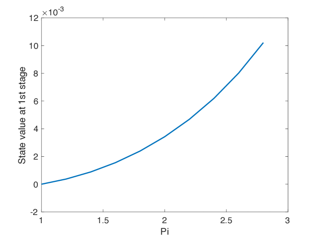
Figure 2: State value at 1st stage in the illustration example.

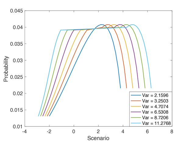
Figure 3: Uncertain price distribution.

6.2 Prudent demand

We then design a case with 24 stages, i.e., $T=24$ (time slots), to verify our theoretical analysis. We set 6 skewed price distributions with increasing variance and the same expectation, and assume that the event happened at the 10th stage. With the same expectation, as the distribution is skewed, a greater variance indicates more skewness in the price distribution. We discretize the price distribution into 30 scenarios with the occurrence probability of each scenario. Fig. 3 shows the detailed price distributions.

We show the 24-stage state value under the 1st price distribution in Fig. 4 (a). The state value at stages 1-9 gradually increases until the event happens at the 10th stage, indicating the demand level change in all the prior stages. This reflects skewness-averse behavior and shows the prudent demand, which will prepare to respond to the event beforehand. The state then changes corresponding to different price scenarios when the event happens.

We use stochastic dynamic programming to solve the problem, and Fig. 4 (b) shows the error curve with iteration number. The error is calculated by the $l_{2}-$norm of state value differences between two nearby iterations, and the algorithm converges when the state doesn’t change. The error curve shows a good convergence performance, and the calculation time is nearly 2s for one price distribution.

Fig. 4 (c) shows the distributional influence on the state value $x_{9}$. The state value at all prior stages increases with the price distribution variance (skewness). More importantly, the increased rate (slope) of state value also increases with the skewness. This indicates that more demand has been prepared ahead of time, and shows the sensitivity of prudent demand, i.e., the degree of skewness aversion.

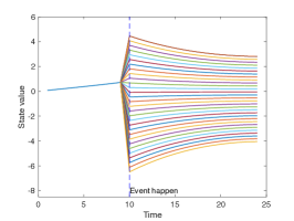
(a) State value under 1st price distribution

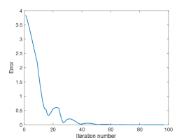
(b) Convergence curve under 1st price distribution

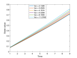
(c) State value under all price distributions

Figure 4: Continuous prudent demand results.

7 Discussion and Conclusion

We provide a theoretical framework to model demand behavior to future volatile electricity prices with a fixed expectation. The proposed framework reveals the distribution-insensitive behavior of demand under future uncertainty when its cost formulation is quadratic. In contrast, demand exhibits prudent behavior when its formulation is super quadratic, in which super quadratic formulation naturally shows higher-order and nonlinear response behavior. Specifically, prudence shows skewness-averse (risk-averse) behavior in response to price uncertainties, in which demand changes its consumption before the price event to prepare for the uncertainty, and this change also increases with the price distribution skewness.

In reality, the demand behavior contributes to many applications. For example, the dynamic pricing tariff mechanism design should consider another demand peak in advance when issuing an incentive-based demand response event for electric vehicles and consumers; bidding strategies designed for battery or virtual power plants should consider the ’pre-preparations’ behavior. Future research will move from the demand model to the agent model, studying the performances of prudent behavior in a multi-agent decision-making framework.

8 Acknowledgement

This work was supported by the National Science Foundation under award ECCS-2239046.

Appendix Appendix A Proof of Theorem 4

Overview of the proof: We derive a series of lemmas that will work for the subsequent analysis. We first derive the formula of the derivative of action-value function $q_{t}(x_{t}|\lambda_{t+1})$ (Lemma 12) and show the relationship between $q_{t}(x_{t}|\lambda_{t+1}),p_{t+1}$ and future price $\lambda_{t+1}$ (Lemma 13). Then, we show the state-value function derivative $v$ is a linear combination of the state cost function derivative $c$ (Lemma 14). Finally, we complete the proof of the Theorem by showing the linear relationship between $q_{t}(x_{t}|\lambda_{t+1})$ and $\lambda_{t+1}$ is necessary and sufficient for the distribution-insensitive demand.

Lemma 12.

Derivative of action-value function. Consider the demand model describe in (3), for all $t\in[0,T-1]$,

$$q_{t}(x_{t}|\lambda_{t+1})=Ah_{t+1}(x_{t+1}).$$ (13)

Proof.

First, we apply the optimality condition to $Q_{t}(x_{t}|\lambda_{t+1})$ to find the minimized $p_{t+1}$,

$$\frac{\partial Q_{t}(x_{t}|\lambda_{t+1})}{\partial p_{t+1}} =\lambda_{t+1}+\frac{\partial C_{t+1}(x_{t+1})}{\partial x_{t+1}}\frac{\partial x_{t+1}}{\partial p_{t+1}}+\frac{\partial V_{t+1}(x_{t+1})}{\partial x_{t+1}}\frac{\partial x_{t+1}}{\partial p_{t+1}}+\frac{\partial G_{t+1}(p_{t+1})}{\partial p_{t+1}}=0,$$ (14)

and according to (1b), $\partial x_{t+1}/\partial p_{t+1}=1$. Then the optimality condition is equivalent to

$$\lambda_{t+1}+g_{t+1}(p_{t+1})+h_{t+1}(x_{t+1})=0,$$ (15a)

$$x_{t+1}=Ax_{t}+p_{t+1}.$$ (15b)

With the optimal $p_{t+1}$, we take derivative for $Q_{t}(x_{t}|\lambda_{t+1})$ with regards to $x_{t}$,

$$\frac{\partial Q_{t}(x_{t}|\lambda_{t+1})}{\partial x_{t}}=\lambda_{t+1}\frac{\partial p_{t+1}}{\partial x_{t}}+\frac{\partial C_{t+1}(x_{t+1})}{\partial x_{t+1}}\frac{\partial x_{t+1}}{\partial x_{t}}+\frac{\partial V_{t+1}(x_{t+1})}{\partial x_{t+1}}\frac{\partial x_{t+1}}{\partial x_{t}}+g_{t+1}(p_{t+1})\frac{\partial p_{t+1}}{\partial x_{t}},$$ (16a)

and according to (1b),

$$\frac{\partial x_{t+1}}{\partial x_{t}}=A+\frac{\partial p_{t+1}}{\partial x_{t}}.$$ (16b)

Thus, combine with (15a) and (16b),

$$q_{t}(x_{t}|\lambda_{t+1}) =\lambda_{t+1}\frac{\partial p_{t+1}}{\partial x_{t}}+h_{t+1}(x_{t+1})\frac{\partial x_{t+1}}{\partial x_{t}}+g_{t+1}(p_{t+1})\frac{\partial p_{t+1}}{\partial x_{t}}$$

$$=\lambda_{t+1}\frac{\partial p_{t+1}}{\partial x_{t}}+h_{t+1}(x_{t+1})(A+\frac{\partial p_{t+1}}{\partial x_{t}})+g_{t+1}(p_{t+1})\frac{\partial p_{t+1}}{\partial x_{t}}$$

$$=\lambda_{t+1}\frac{\partial p_{t+1}}{\partial x_{t}}+h_{t+1}(x_{t+1})(A+\frac{\partial p_{t+1}}{\partial x_{t}})-(\lambda_{t+1}+h_{t+1}(x_{t+1}))\frac{\partial p_{t+1}}{\partial x_{t}}=Ah_{t+1}(x_{t+1}),$$ (16c)

where the optimal $x_{t+1}$ is a function of $\lambda_{t+1}$. ∎

Lemma 12 shows the relationship between $q_{t}(x_{t}|\lambda_{t+1})$ and $h_{t+1}(x_{t+1})$, which provides the basis to analyze the relationship between current action-value function and future price, and motivates us to introduce the following Lemma.

Lemma 13.

Relationship between $p_{t+1},q_{t}(x_{t}|\lambda_{t+1})$ and $\lambda_{t+1}$. Consider the demand model describe in (3), for all $t\in[0,T-1]$,

$$\frac{\partial p_{t+1}}{\partial\lambda_{t+1}}=-\frac{1}{\dot{g}_{t+1}(p_{t+1})+\dot{h}_{t+1}(x_{t+1})},$$ (17a)

$$\frac{\partial q_{t}(x_{t}|\lambda_{t+1})}{\partial\lambda_{t+1}}=A\frac{\partial h_{t+1}(x_{t+1})}{\partial\lambda_{t+1}}=\frac{-A\dot{h}_{t+1}(x_{t+1})}{\dot{g}_{t+1}(p_{t+1})+\dot{h}_{t+1}(x_{t+1})}.$$ (17b)

Proof.

According to the optimality conditions for $p_{t+1}$ as described in (15a),

$$\frac{\partial(g_{t+1}(p_{t+1})+h_{t+1}(x_{t+1}))}{\partial\lambda_{t+1}}=-\frac{\partial\lambda_{t+1}}{\partial\lambda_{t+1}},$$ (18a)

$$\frac{\partial g_{t+1}(p_{t+1})}{\partial p_{t+1}}\frac{\partial p_{t+1}}{\partial\lambda_{t+1}}+\frac{\partial h_{t+1}(x_{t+1})}{\partial x_{t+1}}\frac{\partial x_{t+1}}{\partial p_{t+1}}\frac{\partial p_{t+1}}{\partial\lambda_{t+1}}=-1,$$ (18b)

$$\dot{g}_{t+1}(p_{t+1})\frac{\partial p_{t+1}}{\partial\lambda_{t+1}}+\dot{h}_{t+1}(x_{t+1})\frac{\partial p_{t+1}}{\partial\lambda_{t+1}}=-1,$$ (18c)

$$\frac{\partial p_{t+1}}{\partial\lambda_{t+1}}=-\frac{1}{\dot{g}_{t+1}(p_{t+1})+\dot{h}_{t+1}(x_{t+1})}.$$ (18d)

Then, we take derivative of $q_{t}(x_{t}|\lambda_{t+1})$ with regards to $\lambda_{t+1}$ and combine with Lemma 12,

$$\frac{\partial q_{t}(x_{t}|\lambda_{t+1})}{\partial\lambda_{t+1}} =\frac{\partial Ah_{t+1}(x_{t+1})}{\partial\lambda_{t+1}}=A\frac{\partial h_{t+1}(x_{t+1})}{\partial x_{t+1}}\frac{\partial x_{t+1}}{\partial p_{t+1}}\frac{\partial p_{t+1}}{\partial\lambda_{t+1}}=\frac{-A\dot{h}_{t+1}(x_{t+1})}{\dot{g}_{t+1}(p_{t+1})+\dot{h}_{t+1}(x_{t+1})}.$$ (19)

This completes the proof of the Lemma. ∎

Involving the relationship between $h$ and $x$, Lemma 13 provide an exact relationship between $p_{t+1},q_{t}(x_{t}|\lambda_{t+1})$ and $\lambda_{t+1}$. However, the conditions described in Theorem 4 only state the properties of the $C,G$ rather than $h$ or $v$ with regards to $x$. We then introduce the following Lemma to connect $v$ with $c$.

Lemma 14.

State-value function derivative. The state-value function derivative $v_{t}(x_{t})$ of the demand model described in (3) satisfy the following for all $t\in[1,T]$:

$$v_{t}(x_{t})=\sum_{\tau=t+1}^{T}a_{\tau}c_{\tau}(x_{\tau})+a_{\mathrm{v}}v_{T}(x_{T}),$$ (20)

where $a_{\tau},a_{\mathrm{v}}$ is the parameters for the linear combination.

Proof.

Taking derivative of (3b) with regards to $x_{t}$,

$$v_{t}(x_{t})=\mathbb{E}_{\Lambda_{t+1}}[q_{t}(x_{t}|\lambda_{t+1})],$$ (21)

and according to (16c) from Lemma 12,

$$q_{T-1}(x_{T-1}|\lambda_{T})=Ah_{T}(x_{T})=A(v_{T}(x_{T})+c_{T}(x_{T})).$$ (22a)

Recursively,

$$q_{T-2}(x_{T-2}|\lambda_{T-1})=A(v_{T-1}(x_{T-1})+c_{T-1}(x_{T-1})=A(\mathbb{E}[A(v_{T}(x_{T})+c_{T}(x_{T}))]+c_{T-1}(x_{T-1})).$$ (22b)

Then,

$$v_{t}(x_{t})=\mathbb{E}\bigg{[}a_{t+1}c_{t+1}(x_{t+1})+\mathbb{E}\big{[}a_{t+2}c_{t+2}(x_{t+2})+\dots+\mathbb{E}[a_{T-1}c_{T-1}(x_{T-1})+\mathbb{E}[a_{T}c_{T}(x_{T})+a_{\mathrm{v}}v_{T}(x_{T})]]\big{]}\bigg{]}.$$ (23)

where $a_{\tau},\tau\in[t+1,T]$ and $a_{\mathrm{v}}$ is the constant parameters.

As expectation is a linear transformation, we can write $v_{t}(x_{t})$ as (20) and complete the proof. ∎

Lemma 14 shows the state-value function derivative is a linear combination of state cost function derivative $c$ and end state-value function derivative $v_{T}$. As the model definition mentions, we reasonably set the end state-value function to zero, and finish the proof.

Proof of Theorem 4.

According to Lemma 14, we rewrite the expression of $h_{t+1}=c_{t+1}+v_{t+1}$ as $\sum_{\tau=t+1}^{T}a_{\tau}c_{\tau}$ with an end state-value function of zero. According to the conditions described in Theorem 4, state cost function $C$ and action cost function $G$ is quadratic, then $h$ is a linear function with regard to $x$. Combining with Lemma 13, denote $M_{1},M_{2}$ as a constant, $M_{1},M_{2}\in\mathbb{R}$, $(\partial p_{t+1})/(\partial\lambda_{t+1})=M_{1}$ and $(\partial q_{t}(x_{t}|\lambda_{t+1}))/(\partial\lambda_{t+1})=(\partial h_{t+1}(x_{t+1}))/(\partial\lambda_{t+1})=M_{2}$. This means a linear relationship between both $p_{t+1},\lambda_{t+1}$ and $q_{t}(x_{t}|\lambda_{t+1}),\lambda_{t+1}$.

We first take an example with a two-point price distribution given $w\in[0,1]$,

$$\gamma_{t+1} =\mathbb{E}[\lambda_{t+1}]-w\delta_{t+1}\text{ with a probability of $1-w$},$$ (24a)

$$\pi_{t+1} =\mathbb{E}[\lambda_{t+1}]+(1-w)\delta_{t+1}\text{ with a probability of $w$},$$ (24b)

which ensures the expectation of this two-point price distribution is always $\mathbb{E}[\lambda_{t+1}]$ as $(1-w)\gamma_{t+1}+w\pi_{t+1}=\mathbb{E}[\lambda_{t+1}]$, while with any given $w$, the variance of the distribution scales monotonically with $\delta_{t+1}=\pi_{t+1}-\gamma_{t+1}$.

Then, we take $\lambda_{t+1},\gamma_{t+1}$ into the $q_{t}(x_{t}|\lambda_{t+1})$ expression and explicitly get,

$$(1-w)q_{t}(x_{t}|\gamma_{t+1}) =A(1-w)h_{t+1}(x_{t}+p_{t+1}(\mathbb{E}[\lambda_{t+1}]-w\delta_{t+1}))$$

$$=A(1-w)h_{t+1}(x_{t}+p_{t+1}(\mathbb{E}[\lambda_{t+1}]))-Aw(1-w)h_{t+1}(p_{t+1}(\delta_{t+1})),$$ (25a)

$$wq_{t}(x_{t}|\pi_{t+1}) =Awh_{t+1}(x_{t}+p_{t+1}(\mathbb{E}[\lambda_{t+1}]+(1-w)\delta_{t+1}))$$

$$=Awh_{t+1}(x_{t}+p_{t+1}(\mathbb{E}[\lambda_{t+1}]))+Aw(1-w)h_{t+1}(p_{t+1}(\delta_{t+1})).$$ (25b)

Thus,

$$wq_{t}(x_{t}|\pi_{t+1})+(1-w)q_{t}(x_{t}|\gamma_{t+1})=Ah_{{t+1}}(x_{t}+p_{t+1}(\mathbb{E}[\lambda_{t+1}]))=q_{t}(x_{t}|\mathbb{E}[\lambda_{t+1}]).$$ (26)

Now we consider a general distribution $\Lambda_{t+1}$, and due to the linear relationship between $q_{t}(x_{t}|\lambda_{t+1})$ and $\lambda_{t+1}$, we can write (26) as follows,

$$\mathbb{E}_{\Lambda_{t+1}}[q_{t}(x_{t}|\lambda_{t+1})]=q_{t}(x_{t}|\mathbb{E}_{\Lambda_{t+1}}[\lambda_{t+1}]),$$ (27)

which shows the derivative of the action-value function is distribution-insensitive to the price distribution, but only expectation.

Then we prove (27) is the sufficient and necessary conditions for the distribution-insensitive demand. In terms of the sufficient condition, given (27), when the expectation of price distribution is fixed, $q_{t}$ is insensitive to the price distribution. This means the state-value function derivative $v_{t}$ is the same when taking different distributions at stage $t+1$, so as to the demand action and state at stage $t$.

For the necessary condition, given demand at stage $t$ is insensitive to price distribution at stage $t+1$, then $v_{t}$ and $q_{t}$ are only affected by the expectation instead of the price distributions. This means the expectation can be moved to the price variable ($\mathbb{E}_{\Lambda_{t+1}}[\lambda_{t+1}]$) directly, corresponding to a linear $q_{t}$ function with regards to price $\lambda_{t+1}$, as (27) shows. This completes the proof of Theorem 4. ∎

Appendix Appendix B Proof of Corollary 6

Proof.

We first show the extra case. As the system is linear and cost function formulation is symmetrical, with a prior state of zero ($x_{t-1}=0$) and symmetry price distribution with a mean of zero ($\mathbb{E}_{\Lambda_{t+1}}[\lambda_{t+1}]=0$), demands action should be zero. This shows the distribution-insensitive demand.

We then prove the other parts of the Corollary from three perspectives. The first is the super quadratic state cost function and quadratic action cost function.

From Lemma 13, denote $\alpha_{1}$ as a constant,

$$\frac{\partial h_{t+1}(x_{t+1})}{\partial\lambda_{t+1}}=-\frac{\dot{h}_{t+1}(x_{t+1})}{\alpha_{1}+\dot{h}_{t+1}(x_{t+1})},$$ (28)

Thus, $\partial h_{t+1}(x_{t+1})/\partial\lambda_{t+1}$ is not a constant, and $h_{t+1}(x_{t+1})$ is not a linear function with regard to $\lambda_{t+1}$. According to the proof of Theorem 4, the distribution-insensitive condition doesn’t hold, and the demand model is distribution-sensitive.

Then, we prove the super quadratic action cost function and quadratic state cost function. Also, from Lemma 13, denote $\alpha_{2}$ as a constant,

$$\frac{\partial h_{t+1}(x_{t+1})}{\partial\lambda_{t+1}}=-\frac{\alpha_{2}}{\dot{g}_{t+1}(p_{t+1})},$$ (29)

Following the same analysis, we show the demand model becomes distribution-sensitive. These two cases also show that demand is distribution-sensitive with super quadratic state and action cost function and prove this Corollary. ∎

Appendix Appendix C Proof of Theorem 7

Overview of the proof. In our proof, we set the event to happen at stage $t+1$ and use the price model for stage $t+1$ as described in (5). By model definition, we reasonably set the end state-value function to zero. Here, we only consider the decision behavior before the event at the stage $t+1$ instead of the situation after the event happens, which is independent of the $V_{t+1}(x_{t+1})$; thus, we assume $V_{t+1}(x_{t+1})=0$. We specify the proof process as follows:

• We first assume $V_{t+1}(x_{t+1})=0$ and write the extended form for the first stage optimization problem with price $(\lambda_{\tau}=0,\tau\in[1,t],\gamma_{t+1},\pi_{t+1})$, and take the optimality conditions with regards to actions. Then we write the optimality conditions as a function of the future prices to analyze the optimal solution (Lemma 15).

• We analyze and show the function relationship between price $\gamma_{t+1},\pi_{t+1}$ and optimal state value $x_{t+1}$, and prove its monotonicity, symmetry, and concavity (Lemma 17).

• By using the function property obtained from Lemma 17, we show the $t$th stage reverse state-value function derivative $-v_{t}$ is positive under the optimality condition from Lemma 15 and is greater than the value under the price expectation condition, and the same is true for the state value $x_{t}$ (Lemma 18).

• We further analyze the sensitivity of the reverse state-value function derivative and show that the sate value $x_{t}$ strictly increases with future price $\pi_{t+1}$ (Lemma 19).

Combining these analyses shows that the state value $x_{t}$ is positive, distribution sensitive, and strictly increases with more right skewness price distribution.

Lemma 15.

Demand’s optimality conditions. Taking the price $\gamma_{t+1},\pi_{t+1}$ from distribution $\Lambda_{t+1}$ and demand model described in Theorem 7, assuming $V_{t+1}(x_{t+1})=0$, the optimality conditions for the first stage action of the demand model is:

$$a_{\mathrm{p}}p_{1}+\sum_{\tau=1}^{t}c_{\tau}(x_{\tau})-\mathbb{E}[\lambda_{t+1}]+a_{\mathrm{p}}Ax_{t}-a_{\mathrm{p}}[w_{\Lambda_{t+1}}\phi(-\pi_{t+1}+a_{\mathrm{p}}Ax_{t})+(1-w_{\Lambda_{t+1}})\phi(\gamma_{t+1}+a_{\mathrm{p}}Ax_{t})]=0,$$ (30a)

where $$\phi^{-1}(x_{t+1})=a_{\mathrm{p}}x_{t+1}+c_{t+1}(x_{t+1}) x_{t+1} \lambda_{t+1}$$, describing the function relationship between optimal state and price .

Proof.

According to the demand model define in Theorem 7 and setting $V_{t+1}(x_{t+1})=0$,

$$Q_{t}(x_{t}|\lambda_{t+1})=\min_{p_{t+1}}\lambda_{t+1}p_{t+1}+\frac{a_{\mathrm{p}}}{2}p_{t+1}^{2}+C_{t+1}(x_{t+1}),$$

$$\text{s.t. }x_{t+1}=Ax_{t}+p_{t+1}.$$ (31)

Taking the price scenarios ($\gamma_{t+1},\pi_{t+1}$) inside, we get the state-value function $V_{t}(x_{t})$, (For brevity, we omit the subscript of $w_{\Lambda_{t+1}}$ and express as $w$ without confusion),

$$V_{t}(x_{t})=\mathbb{E}_{\Lambda_{t+1}}[Q_{t}(x_{t}|\lambda_{t+1})] =\min_{p_{\mathrm{\pi},t+1},p_{\mathrm{\gamma},t+1}}w[\pi_{t+1}p_{\mathrm{\pi},t+1}+\frac{a_{\mathrm{p}}}{2}p_{\mathrm{\pi},t+1}^{2}+C_{t+1}(x_{\mathrm{\pi},t+1})]$$

$$+(1-w)[-\gamma_{t+1}p_{\mathrm{\gamma},t+1}+\frac{a_{\mathrm{p}}}{2}p_{\mathrm{\gamma},t+1}^{2}+C_{t+1}(x_{\mathrm{\gamma},t+1})],$$ (32a)

$$\text{s.t. }x_{\mathrm{\pi},t+1} =Ax_{t}+p_{\mathrm{\pi},t+1},$$ (32b)

$$x_{\mathrm{\gamma},t+1} =Ax_{t}+p_{\mathrm{\gamma},t+1},$$ (32c)

where $p_{\mathrm{\pi},t+1},x_{\mathrm{\pi},t+1}$ is the actions and state in stage $t+1$ under price scenario $\pi_{t+1}$; $p_{\mathrm{\gamma},t+1},x_{\mathrm{\gamma},t+1}$ is the actions and state in stage $t+1$ under price scenario $\gamma_{t+1}$.

Thus, we express the optimization problem for the demand recursively starting from the first stage as

$$Q_{0}(x_{0}|\lambda_{\tau,\tau\in[1,t]})=\min_{p_{\mathrm{\gamma},t+1},p_{\mathrm{\pi},t+1},p_{\tau,\tau\in[1,t]}} \sum_{\tau=1}^{t}[\lambda_{\tau}p_{\tau}+\frac{a_{\mathrm{p}}}{2}p_{\tau}^{2}+C_{\tau}(x_{\tau})]$$

$$+w[\pi_{t+1}p_{\mathrm{\pi},t+1}+\frac{a_{\mathrm{p}}}{2}p_{\mathrm{\pi},t+1}^{2}+C_{t+1}(x_{\mathrm{\pi},t+1})] +(1-w)[-\gamma_{t+1}p_{\mathrm{\gamma},t+1}+\frac{a_{\mathrm{p}}}{2}p_{\mathrm{\gamma},t+1}^{2}+C_{t+1}(x_{\mathrm{\gamma},t+1})],$$ (33a)

$$\text{s.t. }x_{\tau} =Ax_{\tau-1}+p_{\tau},\ \forall\tau\in[1,t]$$ (33b)

$$x_{\mathrm{\pi},t+1} =Ax_{t}+p_{\mathrm{\pi},t+1},$$ (33c)

$$x_{\mathrm{\gamma},t+1} =Ax_{t}+p_{\mathrm{\gamma},t+1}.$$ (33d)

Then, we take the optimality conditions for the decision variables, and highlight the conditions of $p_{1},p_{\mathrm{\gamma},t+1},p_{\mathrm{\pi},t+1}$ and take $\lambda_{\tau}=0,\tau\in[1,t]$ inside:

$$p_{1}:a_{\mathrm{p}}p_{1}+\sum_{\tau=1}^{t}c_{\tau}(x_{\tau})+wc_{t+1}(x_{\mathrm{\pi},t+1})+(1-w)c_{t+1}(x_{\mathrm{\gamma},t+1})=0,$$ (34a)

$$p_{\mathrm{\pi},t+1}:\pi_{t+1}+a_{\mathrm{p}}p_{\mathrm{\pi},t+1}+c_{t+1}(x_{\mathrm{\pi},t+1})=0,$$ (34b)

$$p_{\mathrm{\gamma},t+1}:-\gamma_{t+1}+a_{\mathrm{p}}p_{\mathrm{\gamma},t+1}+c_{t+1}(x_{\mathrm{\gamma},t+1})=0,$$ (34c)

among them, (33b)-(33d) also stands with optimal $$x p$$ and .

Then, by multiplying (34b) by $w$, multiplying (34c) by $1-w$, and taking this into (34a), we can rewrite the $t$th stage state-value function derivative in (34a),

$$a_{\mathrm{p}}p_{1} +\sum_{\tau=1}^{t}c_{\tau}(x_{\tau})-w\pi_{t+1}-wa_{\mathrm{p}}p_{\mathrm{\pi},t+1}+(1-w)\gamma_{t+1}-(1-w)a_{\mathrm{p}}p_{\mathrm{\gamma},t+1}=0,$$ (35a)

as $$w\pi_{t+1}-(1-w)\gamma_{t+1}=\mathbb{E}[\lambda_{t+1}]$$,

$$a_{\mathrm{p}}p_{1}+\sum_{\tau=1}^{t} c_{\tau}(x_{\tau})-\mathbb{E}[\lambda_{t+1}]-a_{\mathrm{p}}[wp_{\mathrm{\pi},t+1}+(1-w)p_{\mathrm{\gamma},t+1}]=0.$$ (35b)

Then, to find the relationships between state-value function derivative $v_{t}$ and price $\lambda,\gamma,\pi$, we replace the action $p_{\mathrm{\pi},t+1}$ and $p_{\mathrm{\gamma},t+1}$ in (35b) as the price $\pi_{t+1}$ and $\gamma_{t+1}$, respectively. We connect the price with optimal action/state according to (34b),

$$\pi_{t+1} =-a_{\mathrm{p}}p_{\mathrm{\pi},t+1}-c_{t+1}(x_{\mathrm{\pi},t+1})=-a_{\mathrm{p}}x_{\mathrm{\pi},t+1}-c_{t+1}(x_{\mathrm{\pi},t+1})+a_{\mathrm{p}}Ax_{t},$$ (36a)

$$\pi_{t+1} -a_{\mathrm{p}}Ax_{t}=-\phi^{-1}(x_{\mathrm{\pi},t+1}),$$ (36b)

$$x_{\mathrm{\pi},t+1} =\phi(-\pi_{t+1}+a_{\mathrm{p}}Ax_{t}),$$ (36c)

where $$\phi^{-1}(x_{t+1})=a_{\mathrm{p}}x_{t+1}+c_{t+1}(x_{t+1})$$.

Applying the same steps to (34c),

$$\gamma_{t+1}+a_{\mathrm{p}}Ax_{t} =a_{\mathrm{p}}x_{\mathrm{\gamma},t+1}+c_{t+1}(x_{\mathrm{\gamma},t+1})=\phi^{-1}(x_{\mathrm{\gamma},t+1}),$$ (36d)

$$x_{\mathrm{\gamma},t+1} =\phi(\gamma_{t+1}+a_{\mathrm{p}}Ax_{t}).$$ (36e)

Then we rewrite (35b) as $x_{t+1}$ expression by adding $Ax_{t}$ and replace $x_{\mathrm{\gamma},t+1},x_{\mathrm{\pi},t+1}$ to the function of price $\gamma_{t+1},\pi_{t+1}$.

$$a_{\mathrm{p}}p_{1}+\sum_{\tau=1}^{t}c_{\tau}(x_{\tau})-\mathbb{E}[\lambda_{t+1}] -a_{\mathrm{p}}[wx_{\mathrm{\pi},t+1}+(1-w)x_{\mathrm{\gamma},t+1}-Ax_{t}]=0,$$ (37a)

$$a_{\mathrm{p}}p_{1}+\sum_{\tau=1}^{t}c_{\tau}(x_{\tau})-\mathbb{E}[\lambda_{t+1}]+a_{\mathrm{p}}Ax_{t} -a_{\mathrm{p}}[w\phi(-\pi_{t+1}+a_{\mathrm{p}}Ax_{t})+(1-w)\phi(\gamma_{t+1}+a_{\mathrm{p}}Ax_{t})]=0.$$ (37b)

Thus, we finish the proof of Lemma 15. ∎

Remark 16.

Optimality conditions with price expectation. Follow Lemma 15, when taking the expectation of price distribution $\Lambda_{t+1}$, which is $\mathbb{E}[\lambda_{t+1}]$, the same optimality conditions of the demand model in Theorem 7 is

$$a_{\mathrm{p}}p_{1}+\sum_{\tau=1}^{t}c_{\tau}(x_{\tau})-\mathbb{E}[\lambda_{t+1}]+a_{\mathrm{p}}Ax_{t}-a_{\mathrm{p}}\phi(-\mathbb{E}[\lambda_{t+1}]+a_{\mathrm{p}}Ax_{t})=0.$$ (38)

An intuitive explanation of this Lemma is to replace the state-value function derivative from state expression $x_{t+1}$ to price expression $(\mathbb{E}[\lambda_{t+1}],\gamma_{t+1},\pi_{t+1})$. The key to analyzing the optimality conditions is to show the function property of $\phi(\lambda)$, which motivates us to provide the following Lemma.

Lemma 17.

Property of $\phi(\lambda)$. The inverse function $\phi(\lambda)$ from $\phi^{-1}(x)$ described in Lemma 15 strictly increases, symmetry about the origin, strictly concave when $\lambda\geq 0$ and strictly convex when $\lambda<0$, and $\phi(0)=0$.

Proof.

By definition, the state cost function $C(x)$ is continuously differentiable, super quadratic, convex, and symmetrical with the y-axis. This means the first-order derivative $c(x)$ is strictly convex when $x\geq 0$ and strictly concave when $x<0$. We also have $c(x)=-c(-x)$ as $c(x)$ is symmetric about the origin.

Then we analyze the property of $\phi^{-1}(x)=c(x)+a_{\mathrm{p}}x$.

• For convexity, the affine function $a_{\mathrm{p}}x$ doesn’t affect the function convexity, so the function convexity is determined by $c(x)$. This means $\phi^{-1}(x)$ is strictly convex when $x\geq 0$ and strictly concave when $x<0$.

• Because the $c(x)$ is strictly increase, $\phi^{-1}(x)$ is strictly increase.

• In terms of the symmetry, as $c(x)$ and $a_{\mathrm{p}}x$ are symmetry about the origin, $\phi^{-1}(x)$ is symmetry about the origin.

• Intuitively, we have $\phi^{-1}(0)=0$

Thus, $\phi^{-1}(x)$ is strictly increase, and strictly convex when $x\geq 0$ and strictly concave when $x<0$, and $\phi^{-1}(x)+\phi^{-1}(-x)=0,\phi^{-1}(0)=0$.

Because the inverse function of a strictly increasing convex function is concave and strictly increased, and the inverse of a strictly increasing concave function is convex and strictly increased, we know $\phi(\lambda)$ strictly increases, strictly concave when $\lambda\geq 0$ and strictly convex when $\lambda<0$, and $\phi(\lambda)+\phi(-\lambda)=0,\phi(0)=0$. This completes the proof of Lemma 17. ∎

The analysis of Lemma 17 implies $\phi(\lambda)$ is a piecewise convex and concave function with central symmetry property. We naturally provide the following Lemma to analyze the $t$th stage state-value function derivative in the optimality conditions from Lemma 15 using the property of this $\phi(\lambda)$ function.

Lemma 18.

Property of reverse state-value function derivative. Consider the $\phi^{-1}(x)$ described in Lemma 15 and its inverse function $\phi(\lambda)$, and take the price model described in Lemma 15, the following properties are true,

1. $a_{\mathrm{p}}\phi(\lambda)-\lambda$ strictly decreases with regards to $\lambda$;

2. The $t$th stage reverse state-value function derivative from Lemma 15 under price distribution $\gamma_{t+1},\pi_{t+1}$ and expectation $\mathbb{E}[\lambda_{t+1}]$ satisfies,

   $$x_{t} >0,$$ (39a)

   $$-q_{t}(x_{t}|\mathbb{E}[\lambda_{t+1}]) =\mathbb{E}[\lambda_{t+1}]-a_{\mathrm{p}}Ax_{t}+a_{\mathrm{p}}\phi(-\mathbb{E}[\lambda_{t+1}]+a_{\mathrm{p}}Ax_{t})>0,$$ (39b)

   $$-\mathbb{E}[q_{t}(x_{t}|\lambda_{t+1})] =\mathbb{E}[\lambda_{t+1}]-a_{\mathrm{p}}Ax_{t}+a_{\mathrm{p}}[w_{\Lambda_{t+1}}\phi(-\pi_{t+1}+a_{\mathrm{p}}Ax_{t})+(1-w_{\Lambda_{t+1}})\phi(\gamma_{t+1}+a_{\mathrm{p}}Ax_{t})]$$

   $$>-q_{t}(x_{t}|\mathbb{E}[\lambda_{t+1}]).$$ (39c)

Proof.

We first prove the property 1).

According to Lemma 15, $\phi^{-1}(x)=c(x)+a_{\mathrm{p}}x$. Denote $\dot{}$ as the first-order derivative in terms of the function variable $x$ or $\lambda$, due to $\dot{c}(x)$ is positive, $\dot{\phi}^{-1}(x)>a_{\mathrm{p}}$, and according to the definition of inverse function, $\dot{\phi}(\lambda)<\frac{1}{a_{\mathrm{p}}}$.

By taking derivative of the $a_{\mathrm{p}}\phi(\lambda)-\lambda$,

$$\frac{\partial(a_{\mathrm{p}}\phi(\lambda)-\lambda)}{\partial\lambda}=a_{\mathrm{p}}\dot{\phi}(\lambda)-1<0.$$ (40)

This means the function $a_{\mathrm{p}}\phi(\lambda)-\lambda$ strictly decreases with regrades to $\lambda$.

Then, we prove the property 2) by contradiction. For brevity, we omit the stage index $(t+1)$ for variables and subscript of $w_{\Lambda_{t+1}}$ when there is no ambiguity.

We first assume $x_{t}\leq 0$. Then, the $-\mathbb{E}[\lambda]+a_{\mathrm{p}}Ax_{t}<0$. Based on Lemma 17, we rewrite (39b) as

$$a_{\mathrm{p}}\phi(\mathbb{E}[\lambda]-a_{\mathrm{p}}Ax_{t})<\mathbb{E}[\lambda]-a_{\mathrm{p}}Ax_{t}.$$ (41)

According to the property 1), $a_{\mathrm{p}}\phi[\mathbb{E}[\lambda]-a_{\mathrm{p}}Ax_{t}]-[\mathbb{E}[\lambda]-a_{\mathrm{p}}Ax_{t}]$ strictly decreases with regrades to $\mathbb{E}[\lambda]-a_{\mathrm{p}}Ax_{t}$, and $\phi(0)=0$. Thus, with $\mathbb{E}[\lambda]-a_{\mathrm{p}}Ax_{t}>0$, (41) stands.

Thus, we prove (41) when assuming $x_{t}\leq 0$. Then we take this property into the optimality conditions from Remark 16,

$$a_{\mathrm{p}}p_{1}+\sum_{\tau=1}^{t}c_{\tau}(x_{\tau})=\mathbb{E}[\lambda]-a_{\mathrm{p}}Ax_{t}+a_{\mathrm{p}}\phi(-\mathbb{E}[\lambda]+a_{\mathrm{p}}Ax_{t}).$$ (42)

As the reverse state-value function derivative (right-hand side) is positive, the left-hand side must be positive,

$$a_{\mathrm{p}}p_{1}+\sum_{\tau=1}^{t}c_{\tau}(x_{\tau})>0.$$ (43)

Because $x_{\tau}=Ax_{\tau-1}+p_{\tau},\forall\tau\in[1,t]$, $x_{0}=0$, according to the objective of the demand model with quadratic action cost and super quadratic state cost, (43) means the state value $x_{t}$ at stage $t$ should be positive, and state and actions at prior stages should be non-negative. The zero actions and states come from the discount factor $A$. This contradicts our assumption of $x_{t}\leq 0$. Thus, we get $x_{t}>0$. Also, following the same process, when $x_{t}>0$, the (39b) should still stand to satisfy the optimality conditions and $-\mathbb{E}[\lambda]+a_{\mathrm{p}}Ax_{t}<0$.

Then, we separate two cases to analyze the (39c).

Case (1): $\gamma+a_{\mathrm{p}}Ax_{t}<0$. Under this condition, after some moderately tedious algebra, we rewrite (39c) as

$$w\phi(\pi-a_{\mathrm{p}}Ax_{t})+(1-w)\phi(-\gamma-a_{\mathrm{p}}Ax_{t})<\phi(\mathbb{E}[\lambda]-a_{\mathrm{p}}Ax_{t}),$$ (44a)

where $$\pi-a_{\mathrm{p}}Ax_{t}>0,-\gamma-a_{\mathrm{p}}Ax_{t}>0,\mathbb{E}[\lambda]-a_{\mathrm{p}}Ax_{t}>0 \phi(\lambda) \lambda\geq 0$$, and is a concave when . Then, according to the Jensen’s inequality of strictly concave function [Boyd and Vandenberghe, 2004],

$$w\phi(\pi-a_{\mathrm{p}}Ax_{t})+(1-w)\phi(-\gamma-a_{\mathrm{p}}Ax_{t})<\phi[w\pi-wa_{\mathrm{p}}Ax_{t}-(1-w)\gamma-(1-w)a_{\mathrm{p}}Ax_{t}]=\phi(\mathbb{E}[\lambda]-a_{\mathrm{p}}Ax_{t}),$$ (44b)

which prove (44a).

Case (2): $\gamma+a_{\mathrm{p}}Ax_{t}\geq 0$. Under this condition, after some moderately tedious algebra, we rewrite (39c) as

$$w\phi(\pi-a_{\mathrm{p}}Ax_{t})-(1-w)\phi(\gamma+a_{\mathrm{p}}Ax_{t})<\phi(\mathbb{E}[\lambda]-a_{\mathrm{p}}Ax_{t})$$ (45)

which is true according to the case (1) analysis.

Combining two cases shows the (39c) is true. Taking this property into the optimality conditions from Lemma 15, we get a greater right-hand side of (42), a greater left-hand side follows, thus resulting in a positive and greater $x_{t}$. This completes the proof of Lemma 18. ∎

Lemma 18 provides important properties of $t$th stage state-value function derivative, helping us analyze the optimality conditions with price $\gamma_{t+1},\pi_{t+1}$ and $\mathbb{E}[\lambda_{t+1}]$. The lack of properties with regards to more skewed price distribution $\Gamma$ motivates us to provide the following Lemma to analyze the sensitivity of $t$th stage state-value function derivative.

Lemma 19.

Sensitivity of reverse state-value function derivative. Given the same conditions of Lemma 18, the following property is true:

• The $t$th stage reverse state-value function derivative from Lemma 15: $-v_{t}(x_{t})=a_{\mathrm{p}}[w_{\Lambda_{t+1}}\phi(-\pi_{t+1}+a_{\mathrm{p}}Ax_{t})+(1-w_{\Lambda_{t+1}})\phi(\gamma_{t+1}+a_{\mathrm{p}}Ax_{t})]+\mathbb{E}[\lambda_{t+1}]-a_{\mathrm{p}}Ax_{t}$ strictly increase with $\pi_{t+1}$.

Proof.

We prove this by showing the derivative of the reverse state-value function derivative $-v_{t}(x_{t})$ with regards to $\pi_{t+1}$ is strictly positive.

From Lemma 18, the following conditions are true (for brevity, we still omit the stage index $(t+1)$ for variables and subscript of $w_{\Lambda_{t+1}}$ when there is no ambiguity.)

$$x_{t}>0,$$ (46a)

$$-\pi+a_{\mathrm{p}}Ax_{t}<0,$$ (46b)

$$\mathbb{E}[\lambda]-a_{\mathrm{p}}Ax_{t}>0.$$ (46c)

According to (46c),

$$w\pi-(1-w)\gamma>a_{\mathrm{p}}Ax_{t},$$ (47a)

$$w\pi-(1-w)\gamma>(1-w)a_{\mathrm{p}}Ax_{t}+wa_{\mathrm{p}}Ax_{t},$$ (47b)

$$w(\pi-a_{\mathrm{p}}Ax_{t})>(1-w)(\gamma+a_{\mathrm{p}}Ax_{t}).$$ (47c)

Due to $w\in[0,0.5]$, $\pi-a_{\mathrm{p}}Ax_{t}>\gamma+a_{\mathrm{p}}Ax_{t}$. Also, by definition, $\gamma+a_{\mathrm{p}}Ax_{t}>-\mathbb{E}[\lambda]+a_{\mathrm{p}}Ax_{t}$, and $\mathbb{E}[\lambda]<\pi$. Thus, let $\chi=-\pi+a_{\mathrm{p}}Ax_{t}<0$, $\alpha=-\gamma-a_{\mathrm{p}}Ax_{t}$, we get $\chi<\alpha<-\chi$. Also, from $w\pi-(1-w)\gamma=\mathbb{E}[\lambda]$,

$$w=\frac{\mathbb{E}[\lambda]+\gamma}{\pi+\gamma},1-w=\frac{\pi-\mathbb{E}[\lambda]}{\pi+\gamma},$$ (48)

Take $w,1-w$ inside and take the derivative of the function with regard to $\pi$,

$$\frac{\partial[w\phi(\chi)+(1-w)\phi(-\alpha)+\mathbb{E}[\lambda]-a_{\mathrm{p}}Ax_{t}]}{\partial\pi}$$

$$=-\frac{\mathbb{E}[\lambda]+\gamma}{(\pi+\gamma)^{2}}\phi(\chi)-\frac{\mathbb{E}[\lambda]+\gamma}{\gamma+\pi}\phi^{\prime}(\chi)+\frac{\mathbb{E}[\lambda]+\gamma}{(\pi+\gamma)^{2}}\phi(-\alpha)=\frac{\mathbb{E}[\lambda]+\gamma}{(\gamma+\pi)^{2}}[\phi(-\alpha)-\phi(\chi)]-\frac{\mathbb{E}[\lambda]+\gamma}{\gamma+\pi}\phi^{\prime}(\chi).$$ (49)

According to the definition of the derivative,

$$\phi^{\prime}(\chi)=\lim_{\alpha\rightarrow\chi}\frac{\phi(\alpha)-\phi(\chi)}{\alpha-\chi}.$$ (50)

Because $\chi<\alpha<-\chi$, and from Lemma 17, $\phi(\lambda)$ is symmetry about the origin, strictly increased, convex and concave when $\lambda<0$ and $\lambda\geq 0$, respectively, and $\phi(0)=0$, we conclude

$$\phi^{\prime}(\chi)\leq\frac{\phi(\chi)-\phi(\alpha)}{\chi-\alpha}<\frac{\phi(\chi)+\phi(\alpha)}{\chi+\alpha}=\frac{-\phi(\alpha)-\phi(\chi)}{-\alpha-\chi},$$ (51)

and the second inequity holds because of the following,

$$(\phi(\chi)-\phi(\alpha))(\chi+\alpha)<(\phi(\chi)+\phi(\alpha))(\chi-\alpha),$$ (52a)

$$\alpha\phi(\chi)<\chi\phi(\alpha),$$ (52b)

$$\phi(\chi)<\phi(\alpha)-\phi^{\prime}(\chi)(\alpha-\chi),$$ (52c)

$$\alpha\phi(\alpha)-\alpha\phi^{\prime}(\chi)(\alpha-\chi)-\chi\phi(\alpha)<0,$$ (52d)

$$(\alpha-\chi)\phi(\alpha)<\alpha\phi^{\prime}(\chi)(\alpha-\chi),$$ (52e)

$$\phi(\alpha)<\alpha\phi^{\prime}(\chi),$$ (52f)

$$\frac{\phi(\alpha)-\phi(0)}{\alpha-0}>\phi^{\prime}(\chi).$$ (52g)

As $\phi(\lambda)$ symmetry about the origin, we know $-\phi(\alpha)=\phi(-\alpha)$ and

$$\phi^{\prime}(\chi)<\frac{\phi(-\alpha)-\phi(\chi)}{-\alpha-\chi}=\frac{\phi(-\alpha)-\phi(\chi)}{\gamma+a_{\mathrm{p}}Ax_{t}-(-\pi+a_{\mathrm{p}}Ax_{t})}=\frac{\phi(-\alpha)-\phi(\chi)}{\gamma+\pi},$$ (53)

which means the sign of (49) is positive.

Thus, we show the first-order derivative of the reverse state-value function derivative $-v_{t}(x_{t})$ with regards to $\pi$ (as (49) shows) is positive. This implies that the reverse state-value function derivative strictly increases with $\pi$, and complete the proof of Lemma 19. ∎

Lemma 19 indicates that with an increased price $\pi_{t+1}$, i.e., $\pi^{\prime}_{t+1}$, the $t$th stage reverse state-value function derivative increase, i.e., right-hand side in the optimality conditions described in (42). This implies the left-hand side also increases; thus, $x_{t}$ increases. By combining all these properties, we are able to complete the proof of Theorem 7.

Proof.

Proof of Theorem 7. First, from Lemma 15, the optimality conditions of the demand model for the first stage action can be expressed as (30). Note that we set $V_{t+1}(x_{t+1})=0$ as it doesn’t affect the action and state before stage $t+1$. We rewrite part of it here for convenience

$$a_{\mathrm{p}}p_{1}+\sum_{\tau=1}^{t}c_{\tau}(x_{\tau})=\mathbb{E}[\lambda_{t+1}]-a_{\mathrm{p}}Ax_{t}+a_{\mathrm{p}}[w_{\Lambda_{t+1}}\phi(-\pi_{t+1}+a_{\mathrm{p}}Ax_{t})+(1-w_{\Lambda_{t+1}})\phi(\gamma_{t+1}+a_{\mathrm{p}}Ax_{t})].$$ (54)

According to Lemmas 17, 18, the right-hand side (reverse state-value function derivative) is positive, and greater than the optimality conditions under price expectation in Remark 16, indicating the positive and greater left-hand side in (54), so as to the $x_{t}$. Also, from Lemma 19, the right-hand side strictly increases with the $\pi_{t+1}$, and the left-hand side follows. Thus, we get the following property for the state-value function,

$$\mathbb{E}_{\Gamma_{t+1}}[Q_{t}(x_{t}|\lambda_{t+1})]>\mathbb{E}_{\Lambda_{t+1}}[Q_{t}(x_{t}|\lambda_{t+1})]>Q_{t}(x_{t}|\mathbb{E}_{\Lambda_{t+1}}[\lambda_{t+1}])>0.$$ (55)

By the model definition, $x_{\tau}=Ax_{\tau-1}+p_{\tau},\tau\in[1,t]$, $x_{0}=0$, the influence of $x_{t}$ degrades following the state transition with a discount factor of $A<1$. Also, the demand has a minimization objective with quadratic action cost and super quadratic state cost. Thus, all actions and states prior to the stage $t$ should be non-negative and non-decreased with the price skewness. This means that price skewness causes higher or equal demand levels to change ahead of time, and this proves the Theorem. ∎

Appendix Appendix D Proof of Corollary 11

Proof.

The key to analyzing this Corollary is the price distributions that satisfy the Corollary 11 can always be discretized as a combination of different two-point price pairs as described in Theorem 7.

We first express the state-value function with price distribution $\Lambda$ as follows: (for brevity, we omit the stage index $t+1$ without ambiguity)

$$\mathbb{E}_{\Lambda}[Q_{t}(x_{t}|\lambda)]=\int_{\lambda\in\mathcal{X}}f_{\Lambda}(\lambda)Q_{t}(x_{t}|\lambda)d\lambda,$$ (56a)

where we separate the integral into two parts with price variable $$\gamma \pi_{\Lambda}$$ and , and get

$$\mathbb{E}_{\Lambda}[Q_{t}(x_{t}|\lambda)]=\int_{-\infty}^{\mu}f_{\Lambda}(\gamma)Q_{t}(x_{t}|\gamma)d\gamma+\int_{\mu}^{+\infty}f_{\Lambda}(\pi_{\Lambda})Q_{t}(x_{t}|\pi_{\Lambda})d\pi_{\Lambda},$$ (56b)

and the same expression stands for distribution $$\Gamma$$:

$$\mathbb{E}_{\Gamma}[Q_{t}(x_{t}|\lambda)]=\int_{-\infty}^{\mu}f_{\Gamma}(\gamma)Q_{t}(x_{t}|\gamma)d\gamma+\int_{\mu}^{+\infty}f_{\Gamma}(\pi_{\Gamma})Q_{t}(x_{t}|\pi_{\Gamma})d\pi_{\Gamma}.$$ (56c)

Then, we discretize the two-point price variables to many two-point price pairs (denoted with superscript $*$) with $w_{\Gamma},1-w_{\Gamma}$ and $w_{\Lambda},1-w_{\Lambda}$ probability, and satisfy expectation condition (9a) $w_{\Gamma}\pi^{*}_{\Gamma}+(1-w_{\Gamma})\gamma^{*}=w_{\Lambda}\pi^{*}_{\Lambda}+(1-w_{\Lambda})\gamma^{*}=\mu$. From conditions (9b)-(9e), $\pi^{*}_{\Gamma}>\pi^{*}_{\Lambda}$, $w_{\Gamma},w_{\Lambda}\in[0,0.5]$, aligning with the price model in Theorem 7. Here we show the right skewness condition, and the left skewness case can be obtained as a mirror, as mentioned in Remark 8. Then, each price pair should follow the same probability distribution as the variables $\gamma,\pi_{\Gamma}$ ($f_{\Gamma}$) and $\gamma,\pi_{\Lambda}$ ($f_{\Lambda}$), respectively, i.e.,

$$\frac{f_{\Gamma}(\pi_{\Gamma}^{*})}{f_{\Gamma}(\gamma^{*})+f_{\Gamma}(\pi^{*}_{\Gamma})}=w_{\Gamma},\frac{f_{\Lambda}(\pi_{\Lambda}^{*})}{f_{\Lambda}(\gamma^{*})+f_{\Lambda}(\pi^{*}_{\Lambda})}=w_{\Lambda},\forall\gamma^{*}\in\gamma,\pi_{\Gamma}^{*}\in\pi_{\Gamma},\pi_{\Lambda}^{*}\in\pi_{\Lambda},$$ (57)

and the expectation of all two-point price pairs is equivalent to the following with the PDF:

$$\frac{f_{\Gamma}(\gamma^{*})\gamma^{*}}{f_{\Gamma}(\pi_{\Gamma}^{*})+f_{\Gamma}(\gamma^{*})}+\frac{f_{\Gamma}(\pi_{\Gamma}^{*})\pi_{\Gamma}^{*}}{f_{\Gamma}(\pi_{\Gamma}^{*})+f_{\Gamma}(\gamma^{*})}=\frac{f_{\Lambda}(\gamma^{*})\gamma^{*}}{f_{\Lambda}(\pi_{\Lambda}^{*})+f_{\Lambda}(\gamma^{*})}+\frac{f_{\Lambda}(\pi_{\Lambda}^{*})\pi_{\Lambda}^{*}}{f_{\Lambda}(\pi_{\Lambda}^{*})+f_{\Lambda}(\gamma^{*})}=\mu.$$ (58)

According to our analysis of the discretization, all the two-point price pairs from $\Gamma,\Lambda$ distribution have the same expectations, $\pi^{*}_{\Gamma}>\pi_{\Lambda}^{*}$, and $w_{\Gamma},w_{\Lambda}\in[0,0.5]$, which satisfy the price model described in Theorem 7. Thus, all price pairs satisfy:

$$(1-w_{\Gamma})Q_{t}(x_{t}|\gamma^{*})+w_{\Gamma}Q_{t}(x_{t}|\pi^{*}_{\Gamma})>(1-w_{\Lambda})Q_{t}(x_{t}|\gamma^{*})+w_{\Lambda}Q_{t}(x_{t}|\pi^{*}_{\Lambda}),$$ (59a)

taking (57) into (59a),

$$\frac{Q_{t}(x_{t}|\gamma^{*})f_{\Gamma}(\gamma^{*})+f_{\Gamma}(\pi_{\Gamma}^{*})Q_{t}(x_{t}|\pi^{*}_{\Gamma})}{f_{\Gamma}(\pi_{\Gamma}^{*})+f_{\Gamma}(\gamma^{*})}>\frac{Q_{t}(x_{t}|\gamma^{*})f_{\Lambda}(\gamma^{*})+f_{\Lambda}(\pi_{\Lambda}^{*})Q_{t}(x_{t}|\pi^{*}_{\Lambda})}{f_{\Lambda}(\pi_{\Lambda}^{*})+f_{\Gamma}(\gamma^{*})}.$$ (59b)

Given the condition (9f), $f_{\Gamma}(\pi_{\Gamma}^{*})+f_{\Gamma}(\gamma^{*})>f_{\Lambda}(\pi_{\Lambda}^{*})+f_{\Gamma}(\gamma^{*})$. Thus, for $\forall\gamma^{*}\in\gamma,\pi_{\Gamma}^{*}\in\pi_{\Gamma},\pi_{\Lambda}^{*}\in\pi_{\Lambda}$,

$$f_{\Gamma}(\gamma^{*})Q_{t}(x_{t}|\gamma^{*})+f_{\Gamma}(\pi_{\Gamma}^{*})Q_{t}(x_{t}|\pi^{*}_{\Gamma})>f_{\Lambda}(\gamma^{*})Q_{t}(x_{t}|\gamma^{*})+f_{\Lambda}(\pi_{\Lambda}^{*})Q_{t}(x_{t}|\pi^{*}_{\Lambda}).$$ (60)

Now, by combining all price pairs,

$$\int_{-\infty}^{+\infty}f_{\Gamma}(\gamma)Q_{t}(x_{t}|\gamma)d\gamma+\int_{-\infty}^{+\infty}f_{\Gamma}(\pi_{\Gamma})Q_{t}(x_{t}|\pi_{\Gamma})d\pi_{\Gamma}>\int_{-\infty}^{+\infty}f_{\Lambda}(\gamma)Q_{t}(x_{t}|\gamma)d\gamma+\int_{-\infty}^{+\infty}f_{\Lambda}(\pi_{\Lambda})Q_{t}(x_{t}|\pi_{\Lambda})d\pi_{\Lambda}.$$ (61a)

Due to $$\gamma<\mu,\pi_{\Gamma}\geq\mu,\pi_{\Lambda}\geq\mu$$,

$$\int_{-\infty}^{\mu}f_{\Gamma}(\gamma)Q_{t}(x_{t}|\gamma)d\gamma+\int_{\mu}^{+\infty}f_{\Gamma}(\pi_{\Gamma})Q_{t}(x_{t}|\pi_{\Gamma})d\pi_{\Gamma}>\int_{-\infty}^{\mu}f_{\Lambda}(\gamma)Q_{t}(x_{t}|\gamma)d\gamma+\int_{\mu}^{+\infty}f_{\Lambda}(\pi_{\Lambda})Q_{t}(x_{t}|\pi_{\Lambda})d\pi_{\Lambda},$$ (61b)

and from (56b) and (56c),

$$\mathbb{E}_{\Gamma}[Q_{t}(x_{t}|\lambda)]>\mathbb{E}_{\Lambda}[Q_{t}(x_{t}|\lambda)]$$ (61c)

which shows given the price distribution conditions as (9), demand shows prudence and proves this Corollary.

∎

References

- [Ameren, nd] Ameren (n.d.). Power smart pricing plan. https://www.ameren.com/illinois/account/customer-service/bill/power-smart-pricing/.
- [Antonopoulos et al., 2021] Antonopoulos, I., Robu, V., Couraud, B., and Flynn, D. (2021). Data-driven modelling of energy demand response behaviour based on a large-scale residential trial. Energy and AI, 4:100071.
- [Berger, 2016] Berger, L. (2016). The impact of ambiguity and prudence on prevention decisions. Theory and Decision, 80:389–409.
- [Borenstein, 2016] Borenstein, S. (2016). The economics of fixed cost recovery by utilities. The Electricity Journal, 29(7):5–12.
- [Boyd and Vandenberghe, 2004] Boyd, S. P. and Vandenberghe, L. (2004). Convex optimization. Cambridge university press.
- [Burger et al., 2019] Burger, S., Schneider, I., Botterud, A., and Pérez-Arriaga, I. (2019). Fair, equitable, and efficient tariffs in the presence of distributed energy resources. Consumer, Prosumer, Prosumager: How Service Innovations will Disrupt the Utility Business Model, 155.
- [Chen et al., 2012] Chen, L., Li, N., Jiang, L., and Low, S. H. (2012). Optimal demand response: Problem formulation and deterministic case. Control and optimization methods for electric smart grids, pages 63–85.
- [ConEd, nd] ConEd (n.d.). Con edison time-of-use rates. https://www.coned.com/en/accounts-billing/your-bill/time-of-use.
- [Deng et al., 2015] Deng, R., Yang, Z., Chow, M.-Y., and Chen, J. (2015). A survey on demand response in smart grids: Mathematical models and approaches. IEEE Transactions on Industrial Informatics, 11(3):570–582.
- [Douglas and Foxhall, 2023] Douglas, E. and Foxhall, E. (2023). Appeals court says state agency set electricity prices too high during 2021 winter storm. The Texas Tribune. https://www.texastribune.org/2023/03/17/puc-appeals-court-uri-prices/.
- [Ebert, 2020] Ebert, S. (2020). Decision making when things are only a matter of time. Operations Research, 68(5):1564–1575.
- [Ebert and Wiesen, 2011] Ebert, S. and Wiesen, D. (2011). Testing for prudence and skewness seeking. Management Science, 57(7):1334–1349.
- [Ebert and Wiesen, 2014] Ebert, S. and Wiesen, D. (2014). Joint measurement of risk aversion, prudence, and temperance. Journal of Risk and Uncertainty, 48:231–252.
- [Eeckhoudt et al., 2016] Eeckhoudt, L., Fiori, A. M., and Gianin, E. R. (2016). Loss-averse preferences and portfolio choices: An extension. European Journal of Operational Research, 249(1):224–230.
- [Eeckhoudt and Schlesinger, 2006] Eeckhoudt, L. and Schlesinger, H. (2006). Putting risk in its proper place. American Economic Review, 96(1):280–289.
- [Ercot, nd] Ercot (n.d.). Real-time market. https://www.ercot.com/mktinfo/rtm/.
- [Giulia et al., 2021] Giulia, M. N. d. R., Nicholas, B.-B., and Ivan, P. (2021). His lights stayed on during texas’ storm. now he owes $16,752. New York Times. https://www.nytimes.com/2021/02/20/us/texas-storm-electric-bills.html\#commentsContainer.
- [Jia and Tong, 2012] Jia, L. and Tong, L. (2012). Optimal pricing for residential demand response: A stochastic optimization approach. In 2012 50th Annual Allerton Conference on Communication, Control, and Computing (Allerton), pages 1879–1884. IEEE.
- [Jia and Tong, 2016] Jia, L. and Tong, L. (2016). Dynamic pricing and distributed energy management for demand response. IEEE Transactions on Smart Grid, 7(2):1128–1136.
- [Jordehi, 2019] Jordehi, A. R. (2019). Optimisation of demand response in electric power systems, a review. Renewable and sustainable energy reviews, 103:308–319.
- [Khan et al., 2023] Khan, H. A. U., Ünel, B., and Dvorkin, Y. (2023). Electricity tariff design via lens of energy justice. Omega, 117:102822.
- [Kimball, 1989] Kimball, M. S. (1989). Precautionary saving in the small and in the large.
- [Kwac and Rajagopal, 2015] Kwac, J. and Rajagopal, R. (2015). Data-driven targeting of customers for demand response. IEEE Transactions on Smart Grid, 7(5):2199–2207.
- [Li and Peter, 2021] Li, L. and Peter, R. (2021). Should we do more when we know less? the effect of technology risk on optimal effort. Journal of Risk and Insurance, 88(3):695–725.
- [Li et al., 2011] Li, N., Chen, L., and Low, S. H. (2011). Optimal demand response based on utility maximization in power networks. In 2011 IEEE power and energy society general meeting, pages 1–8. IEEE.
- [Li et al., 2017] Li, P., Wang, H., and Zhang, B. (2017). A distributed online pricing strategy for demand response programs. IEEE Transactions on Smart Grid, 10(1):350–360.
- [Liu et al., 2017] Liu, N., Yu, X., Wang, C., Li, C., Ma, L., and Lei, J. (2017). Energy-sharing model with price-based demand response for microgrids of peer-to-peer prosumers. IEEE Transactions on Power Systems, 32(5):3569–3583.
- [Mayrhofer and Schmitz, 2020] Mayrhofer, T. and Schmitz, H. (2020). Prudence and prevention–empirical evidence. Available at SSRN 3969646.
- [Menegatti, 2009] Menegatti, M. (2009). Optimal prevention and prudence in a two-period model. Mathematical Social Sciences, 58(3):393–397.
- [Menegatti, 2014] Menegatti, M. (2014). New results on the relationship among risk aversion, prudence and temperance. European Journal of Operational Research, 232(3):613–617.
- [Menegatti, 2015] Menegatti, M. (2015). New results on high-order risk changes. European Journal of Operational Research, 243(2):678–681.
- [Mieth and Dvorkin, 2019] Mieth, R. and Dvorkin, Y. (2019). Online learning for network constrained demand response pricing in distribution systems. IEEE Transactions on Smart Grid, 11(3):2563–2575.
- [Mohsenian-Rad et al., 2010] Mohsenian-Rad, A.-H., Wong, V. W., Jatskevich, J., Schober, R., and Leon-Garcia, A. (2010). Autonomous demand-side management based on game-theoretic energy consumption scheduling for the future smart grid. IEEE transactions on Smart Grid, 1(3):320–331.
- [Morales-España et al., 2022] Morales-España, G., Martínez-Gordón, R., and Sijm, J. (2022). Classifying and modelling demand response in power systems. Energy, 242:122544.
- [OG&E, nd] OG&E (n.d.). Smarthours. https://www.oge.com/wps/portal/ord/residential/pricing-options/smart-hours.
- [Peter, 2017] Peter, R. (2017). Optimal self-protection in two periods: On the role of endogenous saving. Journal of Economic Behavior & Organization, 137:19–36.
- [PG&E, nd] PG&E (n.d.). Find your best rate plan. https://www.pge.com/en/account/rate-plans/find-your-best-rate-plan.html.
- [Pratt, 1978] Pratt, J. W. (1978). Risk aversion in the small and in the large. In Uncertainty in economics, pages 59–79. Elsevier.
- [Qdr, 2006] Qdr, Q. (2006). Benefits of demand response in electricity markets and recommendations for achieving them. US Dept. Energy, Washington, DC, USA, Tech. Rep, 2006.
- [Reichel et al., 2021] Reichel, L., Schmeiser, H., and Schreiber, F. (2021). Sometimes more, sometimes less: Prudence and the diversification of risky insurance coverage. European Journal of Operational Research, 292(2):770–783.
- [Roveto et al., 2020] Roveto, M., Mieth, R., and Dvorkin, Y. (2020). Co-optimization of var and cvar for data-driven stochastic demand response auction. IEEE Control Systems Letters, 4(4):940–945.
- [Saad et al., 2016] Saad, W., Glass, A. L., Mandayam, N. B., and Poor, H. V. (2016). Toward a consumer-centric grid: A behavioral perspective. Proceedings of the IEEE, 104(4):865–882.
- [Samadi et al., 2010] Samadi, P., Mohsenian-Rad, A.-H., Schober, R., Wong, V. W., and Jatskevich, J. (2010). Optimal real-time pricing algorithm based on utility maximization for smart grid. In 2010 First IEEE international conference on smart grid communications, pages 415–420. IEEE.
- [Shapiro et al., 2021] Shapiro, A., Dentcheva, D., and Ruszczynski, A. (2021). Lectures on stochastic programming: modeling and theory. SIAM.
- [SRP, nd] SRP (n.d.). Salt river project (srp) time-of-use price plan™ (tou). https://www.srpnet.com/price-plans/residential-electric/time-of-use.
- [Tang and Wang, 2019] Tang, R. and Wang, S. (2019). Model predictive control for thermal energy storage and thermal comfort optimization of building demand response in smart grids. Applied Energy, 242:873–882.
- [Vázquez-Canteli and Nagy, 2019] Vázquez-Canteli, J. R. and Nagy, Z. (2019). Reinforcement learning for demand response: A review of algorithms and modeling techniques. Applied energy, 235:1072–1089.
- [Wei et al., 2014] Wei, W., Liu, F., and Mei, S. (2014). Energy pricing and dispatch for smart grid retailers under demand response and market price uncertainty. IEEE transactions on smart grid, 6(3):1364–1374.
- [Zheng et al., 2022] Zheng, N., Jaworski, J., and Xu, B. (2022). Arbitraging variable efficiency energy storage using analytical stochastic dynamic programming. IEEE Transactions on Power Systems, 37(6):4785–4795.