A Differential Equation Approach for Wasserstein GANs and Beyond

Abstract

We propose a new theoretical lens to view Wasserstein generative adversarial networks (WGANs). In our framework, we define a discretization inspired by a distribution-dependent ordinary differential equation (ODE). We show that such a discretization is convergent and propose a viable class of adversarial training methods to implement this discretization, which we call W1 Forward Euler (W1-FE). In particular, the ODE framework allows us to implement persistent training, a novel training technique that cannot be applied to typical WGAN algorithms without the ODE interpretation. Remarkably, when we do not implement persistent training, we prove that our algorithms simplify to existing WGAN algorithms; when we increase the level of persistent training appropriately, our algorithms outperform existing WGAN algorithms in both low- and high-dimensional examples.

1 Introduction

Generative modeling, i.e., the task of generating data given some prespecified samples, is a fundamental problem in machine learning and artificial intelligence. Wasserstein generative adversarial network (WGANs), as first introduced in the pivotal work Arjovsky et al. (2017), are a powerful class of models that seek to solve this problem. WGANs use the well-known adversarial training technique, wherein they train a generator to produce samples and a critic to discriminate between the generated samples and true data. While significant follow-up research into WGANs has focused on improving critic training Petzka et al. (2018) Gulrajani et al. (2017), we are not aware of many breakthroughs in improving generator training.

Recent work Huang and Zhang (2023) has shown that the original GAN training Goodfellow et al. (2014) actually follows the dynamics of an ordinary differential equation (ODE). Specifically, the original GAN solves the gradient flow equation generated by the Jensen-Shannon divergence Huang and Zhang (2023, Proposition 8). Now the question is, can we show an analogous result for WGANs? In this paper, we apply the gradient flow idea to the Wasserstein$-1$ loss and observe that minimizing this loss recursively corresponds to an ODE dynamics, i.e., (3.3) below. This allows us to propose a new algorithm for generative modeling that is numerically tractable and feasible. In particular, the algorithm dictates persistent training for the generator, which accelerates training time as compared to standard WGAN algorithms. Note that the inclusion of persistent training is natural under our ODE framework, but not under the original min-max setup of WGANs.

Our paper is structured as follows:

• In Section $2$, we discuss the necessary mathematical framework for our problem.

• Section $3$ contains an informal discussion of the inspiring gradient flow dynamics.

• In Section $4$, we introduce a discrete time process, inspired by the discussion in Section $3$, that can be easily simulated and prove that this discretization encompasses many well known WGAN algorithms. We also use the discretization to introduce persistent training, which is a way to improve generator training.

• Section $5$ shows the efficacy of persistent training in empirical examples.

2 Mathematical preliminaries

For any Polish space $\mathcal{X}$, we denote by $\mathcal{B}(\mathcal{X})$ the Borel $\sigma$-algebra of $\mathcal{X}$ and by $\mathcal{P}(\mathcal{X})$ the collection of all probability measures defined on $(\mathcal{X},\mathcal{B}(\mathcal{X}))$. Given two Polish spaces $\mathcal{X}$ and $\mathcal{Y}$, $\mu\in\mathcal{P}(\mathcal{X})$, and a Borel $f:\mathcal{X}\to\mathcal{Y}$, we define $f_{\#}\mu\in\mathcal{P}(\mathcal{Y})$, called the pushforward of $\mu$ through $f$, by

$$f_{\#}\mu(B):=\mu(f^{-1}(B))\quad\forall B\in\mathcal{B}(\mathcal{Y}).$$

On the product space $\mathcal{X}\times\mathcal{Y}$, consider the projection operators

$$\pi^{1}(x,y):=x\quad\hbox{and}\quad\pi^{2}(x,y):=y,\qquad\forall(x,y)\in\mathcal{X}\times\mathcal{Y}.$$

Definition 2.1.

Given $\mu\in\mathcal{P}(\mathcal{X})$ and $\nu\in\mathcal{P}(\mathcal{Y})$, a Borel $\mathbf{t}:\mathcal{X}\to\mathcal{Y}$ is called a transport map from $\mu$ to $\nu$ if $\mathbf{t}_{\#}\mu=\nu$. Also, a probability $\gamma\in\mathcal{P}(\mathcal{X}\times\mathcal{Y})$ is called a transport plan from $\mu$ to $\nu$ if $\pi^{1}_{\#}\gamma=\mu$ and $\pi^{2}_{\#}\gamma=\nu$. We denote by $\Gamma(\mu,\nu)$ the collection of all transport plans from $\mu$ to $\nu$.

Now, let us fix $d\in\mathbb{N}$, compact subset $\mathcal{X}\subset\mathbb{R}^{d}$ and denote by $\mathcal{P}_{1}(\mathcal{X})$ the collection of elements in $\mathcal{P}(\mathcal{X})$ with finite first moments, i.e.,

$$\mathcal{P}_{1}(\mathcal{X}):=\bigg{\{}\mu\in\mathcal{P}(\mathcal{X}):\int_{\mathbb{R}^{d}}|y|d\mu(y)<\infty\bigg{\}}.$$

The first-order Wasserstein distance, a metric on $\mathcal{P}_{1}(\mathcal{X})$, is defined by

$$W_{1}(\mu,\nu):=\inf_{\gamma\in\Gamma(\mu,\nu)}\int_{\mathcal{X}\times\mathcal{X}}|x-y|\,d\gamma(x,y),\quad\forall\mu,\nu\in\mathcal{P}_{1}(\mathcal{X}).$$ (2.1)

Let us also recall the useful Kantorovich-Rubinstein duality formula for the $W_{1}$ distance. By Villani (2009, Theorem 5.10)

$$W_{1}(\mu_{t},\mu^{d}) = \sup_{||\varphi||_{Lip}\leq 1}\left\{\int_{\mathcal{X}}\varphi(x)\,d\mu^{d}(x)-\int_{\mathcal{X}}\varphi(y)\,d\mu_{t}(y)\right\},$$ (2.2)

where $||\varphi||_{\operatorname{Lip}}$ refers to the Lipschitz constant of the function $\phi$.

Definition 2.2.

Given $\mu,\nu\in\mathcal{P}_{1}(\mathcal{X})$, a minimizing $\gamma\in\Gamma(\mu,\nu)$ for (2.1) is called an optimal transport plan from $\mu$ to $\nu$ and we denote by $\Gamma_{0}(\mu,\nu)$ the collection of all such plans. In addition, a maximizing $1$-Lipschitz $\varphi\in L^{1}(\mathcal{X},\mu)$ for (2.2) is called a (maximal) Kantorovich potential from $\mu$ to $\nu$ and will often be denoted by $\varphi_{\mu}^{\nu}$ to emphasize its dependence on $\mu$ and $\nu$.

Remark 2.1.

The $1$-Lipschitzness of $\varphi_{\mu}^{\nu}$ implies that $\nabla\varphi_{\mu}^{\nu}(x)$ exists for $\mathcal{L}^{d}$-a.e.  $x\in\mathcal{X}$.

Remark 2.2.

For any $\mu,\nu\in\mathcal{P}_{1}(\mathcal{X})$, suppose additionally that $\mu$ belongs to

$$\mathcal{P}_{1}^{r}(\mathcal{X}):=\{\mu\in\mathcal{P}_{1}(\mathcal{X}):\mu\ll\mathcal{L}^{d}\}.$$

Then, by Ambrosio (2000, Theorem 6.2), there is an optimal transport plan $\gamma\in\mathcal{P}(\mathcal{X}\times\mathcal{X})$ which takes the form

$$\gamma=(\mathbf{i}\times\mathbf{t}_{\mu}^{\nu})_{\#}\mu$$ (2.3)

for some transport map $\mathbf{t}_{\mu}^{\nu}:\mathcal{X}\to\mathcal{X}$ from $\mu$ to $\nu$.

Definition 2.3.

Let $\gamma\in\Gamma_{0}(\mu,\nu)$ be the optimal transport plan of the form (2.3). We say that the line segment $]x,y[$ is a transport ray if $x\neq y$ and $(x,y)\in\operatorname{supp}(\gamma)$. The union of transport rays is called the transport set, which we denote by $\mathcal{T}$.

By the characterization (2.3), if $(x,y)\in\operatorname{supp}(\gamma)$, then we clearly have $y=\mathbf{t}_{\mu}^{\nu}(x)$. As such, the transport ray from $x\in\mathcal{X}$ to $\mathbf{t}_{\mu}^{\nu}(x)\in\mathcal{X}$ can be expressed as

$$\{x+s(\mathbf{t}_{\mu}^{\nu}(x)-x)\},\quad s\in(0,1).$$

Remark 2.3.

For any $z\in\mathcal{T}$, by Ambrosio (2000, Proposition 4.2), we know that $\varphi_{\mu}^{\nu}$ is differentiable at $z$, the transport ray containing $z$ is unique, and $-\nabla\varphi_{\mu}^{\nu}(z)$ is the unit vector parallel to the transport ray that contains $z$.

Remark 2.4.

We will call $\mathbf{t}_{\mu}^{\nu}:\mathbb{R}^{d}\to\mathbb{R}^{d}$ in (2.3) an optimal transport map from $\mu$ to $\nu$. Indeed, as $\gamma=(\mathbf{i}\times\mathbf{t}_{\mu}^{\nu})_{\#}\mu$ is an optimal transport plan from $\mu$ to $\nu$, we deduce from (2.1) immediately that

$$W_{1}(\mu,\nu)=\int_{\mathbb{R}^{d}}|\mathbf{t}_{\mu}^{\nu}(x)-x|^{2}\,d\mu(x)=\inf_{\mathbf{t}:\mathbb{R}^{d}\to\mathbb{R}^{d},\mathbf{t}_{\#}\mu=\nu}\int_{\mathbb{R}^{d}}|\mathbf{t}(x)-x|\,d\mu(x).$$

Finally, let us recall a special kind of derivative on the space $\mathcal{P}_{1}(\mathcal{X})$ that will help us justify our theoretical framework. The following definition is adapted from Jourdain and Tse (2021, Definition 2.1)

Definition 2.4.

A linear functional derivative of $U:\mathcal{P}_{1}(\mathcal{X})\rightarrow\mathbb{R}$ is a function $\frac{\delta U}{\delta m}:\mathcal{P}_{1}(\mathcal{X})\times\mathbb{R}^{d}\to\mathbb{R}^{d}$ that satisfies

$$\lim_{\epsilon\rightarrow 0^{+}}\frac{U(\mu+\epsilon(\nu-\mu))-U(\mu)}{\epsilon}=\int_{\mathcal{X}}\frac{\delta U}{\delta m}(\mu,y)\,d(\nu-\mu),\quad\forall\mu,\nu\in\mathcal{P}_{1}(\mathcal{X}).$$ (2.4)

3 Problem formulation

Let $\mu_{\operatorname{d}}\in\mathcal{P}_{1}(\mathcal{X})$ denote the (unknown) data distribution. Starting with an arbitrary initial guess $\mu_{0}\in\mathcal{P}_{1}(\mathcal{X})$ for $\mu_{\operatorname{d}}$, we aim to solve the problem

$$\min_{\mu\in\mathcal{P}_{1}(\mathcal{X})}W_{1}(\mu,\mu_{\operatorname{d}})$$ (3.1)

in an efficient manner. As it can be checked directly that $\mu\mapsto W_{1}(\mu,\mu_{\operatorname{d}})$ is strictly convex on $\mathcal{P}_{1}(\mathcal{X})$, it is natural to ask if (3.1) can be solved simply by gradient descent, the traditional wisdom of convex minimization. The crucial question now is how the “gradient” of the function

$$J(\mu):=W_{1}(\mu,\mu_{d}),\quad\mu\in\mathcal{P}_{1}(\mathcal{X})$$

should be defined. As $\mathcal{P}_{1}(\mathcal{X})$ is not even a vector space, differentiation cannot be easily defined in the usual Fréchet or Gateaux sense. While the subdifferential calculus for probability measures is well-developed in Ambrosio et al. (2008), it is not general enough to cover the entirety of $\mathcal{P}_{1}(\mathcal{X})$. Recently, Huang and Zhang (2023, Section 2) suggested that for a function $U:\mathcal{P}(\mathcal{X})\to\mathbb{R}$, where $\mathcal{P}(\mathcal{X})$ denotes the space of all probability measures, we should take its gradient to be the “Euclidean gradient of its linear functional derivative.” This is because at each $\mu\in\mathcal{P}(\mathcal{X})$, $y\mapsto\nabla\frac{\delta U}{\delta m}(\mu,y)$ satisfies a gradient-type property; see Huang and Zhang (2023, Proposition 5). This means that the gradient-descent ODE for (3.1) can be stated as

$$dY_{t}=-\nabla\frac{\delta J}{\delta m}(\mu^{Y_{t}},Y_{t})\,dt,\quad\mu^{Y_{0}}=\mu_{0}\in\mathcal{P}_{1}(\mathcal{X}).$$ (3.2)

This ODE is distribution-dependent in nontrivial ways. At time 0, $Y_{0}$ is an $\mathbb{R}^{d}$-valued random variable whose law is given by $\mu_{0}\in\mathcal{P}_{1}(\mathcal{X})$, an arbitrarily specified initial distribution. This initial randomness trickles through the ODE dynamics in (3.2), such that $Y_{t}$ remains an $\mathbb{R}^{d}$-valued random variable, with its law denoted by $\mu^{Y_{t}}\in\mathcal{P}_{1}(\mathcal{X})$, at every $t>0$. The evolution of the ODE is then determined jointly by the Euclidean gradient of $J$’s linear functional derivative (i.e., the function $\nabla\frac{\delta J}{\delta m}(\mu^{Y_{t}},\cdot))$ and the actual realization of $Y_{t}$ (which is plugged into $\nabla\frac{\delta J}{\delta m}(\mu^{Y_{t}},\cdot)$).

To make ODE (3.2) more tractable, we compute $\frac{\delta J}{\delta m}$.

Proposition 3.1.

The linear functional derivative of $J:\mathcal{P}_{1}(\mathcal{X})\rightarrow\mathbb{R}$ at $\mu\in\mathcal{P}_{1}(\mathcal{X})$ is the Kantorovich potential $\varphi_{\mu}^{\mu_{d}}$; namely, for any $\mu\in\mathcal{P}_{1}(\mathcal{X})$,

$$\frac{\delta J}{\delta m}(\mu,y)=\varphi_{\mu}^{\mu_{d}}(y)\quad\forall y\in\mathbb{R}^{d}.$$

Proof.

Consider arbitrary $\nu\in\mathcal{P}_{1}(\mathcal{X})$, we wish to compute

$$\lim_{\epsilon\rightarrow 0^{+}}\frac{J(\mu+\epsilon(\nu-\mu))-J(\mu)}{\epsilon}.$$

Fix $\epsilon\in(0,1)$. We observe, since $\varphi_{\mu}^{\mu_{d}}$ is $1$-Lipschitz, that

$$J(\mu+\epsilon(\nu-\mu))\geq\int_{\mathcal{X}}\varphi_{\mu}^{\mu_{d}}\,d(\mu+\epsilon(\nu-\mu)-\mu_{d}).$$

Therefore, we get the inequality

$$J(\mu+\epsilon(\nu-\mu))-J(\mu) \geq\int_{\mathcal{X}}\varphi_{\mu}^{\mu_{d}}\,d(\mu+\epsilon(\nu-\mu)-\mu_{d})-\int_{\mathcal{X}}\varphi_{\mu}^{\mu_{d}}\,d(\mu-\mu_{d})$$

$$=\epsilon\int_{\mathcal{X}}\varphi_{\mu}^{\mu_{d}}\,d(\mu-\nu).$$

Using a similar argument, we can obtain the converse inequality

$$J(\mu)-J(\mu+\epsilon(\nu-\mu)) \geq\int_{\mathcal{X}}\varphi_{\mu+\epsilon(\nu-\mu)}^{\mu_{d}}\,d(\mu-\mu_{d})-\int_{\mathcal{X}}\varphi_{\mu+\epsilon(\nu-\mu)}^{\mu_{d}}\,d(\mu+\epsilon(\nu-\mu)-\mu_{d})$$

$$=\epsilon\int_{\mathcal{X}}\varphi_{\mu+\epsilon(\nu-\mu)}^{\mu_{d}}\,d(\mu-\nu).$$

Putting these two inequalities together, we have that

$$\int_{\mathcal{X}}\varphi_{\mu}^{\mu_{d}}\,d(\mu-\nu)\leq\frac{J(\mu+\epsilon(\nu-\mu))-J(\mu)}{\epsilon}\leq\int_{\mathcal{X}}\varphi_{\mu+\epsilon(\nu-\mu)}^{\mu_{d}}\,d(\mu-\nu).$$

To obtain (2.4), we simply take limit $\epsilon\rightarrow 0^{+}$, recalling, by (Santambrogio, 2015, Theorem 1.52), that $\varphi_{\mu+\epsilon(\nu-\mu)}^{\mu_{d}}$ converges uniformly to $\varphi_{\mu}^{\mu_{d}}$ as $\epsilon\rightarrow 0^{+}$. ∎

Using the previous result, the ODE (3.2) now becomes

$$dY_{t}=-\nabla\varphi_{\mu^{Y_{t}}}^{\mu_{d}}(Y_{t})\,dt,\quad\mu^{Y_{0}}=\mu_{0}\in\mathcal{P}_{1}(\mathcal{X}).$$ (3.3)

That is, the evolution of the ODE is determined jointly by a Kantorovich potential from the present distribution $\mu^{Y_{t}}$ to $\mu_{\operatorname{d}}$ (i.e., the function $\varphi_{\mu^{Y_{t}}}^{\mu_{\operatorname{d}}}(\cdot)$) and the actual realization of $Y_{t}$ (which is plugged into $\nabla\varphi_{\mu^{Y_{t}}}^{\mu_{\operatorname{d}}}(\cdot)$).

Remark 3.1.

In light of Remark 2.3, we may view (3.3) as transporting mass along the transport rays for $\mu^{Y_{t}}$ and $\mu_{d}$. In other words, the “negative gradient of $J$" (i.e., $-\nabla\frac{\delta J}{\delta m}(\mu^{Y_{t}},\cdot)$ in (3.2)) directs mass from $\mu^{Y_{t}}$ towards that of $\mu_{d}$ along the most efficient path possible. This suggests a deep connection between our gradient flow idea and the Wasserstein$-1$ theory of optimal transportation.

4 A discretization of (3.3)

Let us start with some $\epsilon>0$ and an initial random variable $Y_{0,\epsilon}$ with corresponding law $\mu^{Y_{0,\epsilon}}=\mu_{0}$. Consider the Euler update to the initial random variable using the gradient of the Kantorovich potential

$$Y_{1,\epsilon}:=Y_{0,\epsilon}-\epsilon\nabla\varphi_{\mu^{Y_{0,\epsilon}}}^{\mu_{d}}(Y_{0,\epsilon}).$$

As per our previous discussion, we observe that this is the first step in the Euler discretization of the ODE (3.3). Using the law of $Y_{1,\epsilon}$, denoted by $\mu^{Y_{1,\epsilon}}$, we can obtain another Kantorovich potential $\varphi_{\mu^{Y_{1,\epsilon}}}^{\mu_{d}}$ and perform the Euler update

$$Y_{2,\epsilon}:=Y_{1,\epsilon}-\epsilon\nabla\varphi_{\mu^{Y_{1,\epsilon}}}^{\mu_{d}}(Y_{1,\epsilon}).$$

We may proceed inductively and obtain a process $\{Y_{n,\epsilon}\}$ such that

$$Y_{n+1,\epsilon}:=Y_{n,\epsilon}-\epsilon\nabla\varphi_{\mu^{Y_{n,\epsilon}}}^{\mu_{d}}(Y_{n,\epsilon}).$$ (4.1)

Observe that this discretization recursively defines a collection of measures $\{\mu^{Y_{n,\epsilon}}\}\subset\mathcal{P}_{1}(\mathcal{X})$, for $n\in\mathbb{N}$ and $\epsilon\in(0,\epsilon_{0})$ for some $\epsilon_{0}>0$ small enough. We should also note that regardless of the well-posedness of (3.3), the process $\{Y_{n,\epsilon}\}$ generated by (4.1) is always well defined. Let us define the piecewise constant $\mu_{\epsilon}:[0,\infty)\rightarrow\mathcal{P}_{1}(\mathcal{X})$ by

$$\mu_{\epsilon}(t):=\mu^{Y_{n-1,\epsilon}}\quad t\in[(n-1)\epsilon,n\epsilon),\quad n\in\mathbb{N}$$ (4.2)

Now we state our main convergence result. A complete proof is provided in the appendix.

Theorem 4.1.

Let $\mu_{\epsilon}:[0,\infty)\rightarrow\mathcal{P}_{1}(\mathbb{R}^{d})$ be defined as in (4.2). Then, there exists a subsequence $\{\epsilon_{k}\}\subset(0,\epsilon_{0})$ and a curve $\mu^{*}:[0,\infty)\rightarrow\mathcal{P}_{1}(\mathbb{R}^{d})$ such that

$$\lim_{k\rightarrow\infty}W_{1}(\mu_{\epsilon_{k}}(t),\mu^{*}(t))=0$$

Furthermore, $t\mapsto\mu^{*}(t)$ is uniformly continuous (in the $W_{1}$ sense) on compacts of $[0,\infty)$.

Remark 4.1.

It should be noted that this convergence result is especially useful for numerical purposes: we know that this scheme is stable for small time steps and there is a well defined limiting curve.

With this convergence result, we know that the Euler scheme (4.1) is well posed and that a numerical implementation of such a scheme is stable for small time step. We propose to simulate (4.1) using an algorithm we call W1-FE, as shown in Algorithm 1. We use two neural networks to carry out the simulation, one for the Kantorovich potential $\varphi:\mathcal{X}\rightarrow\mathbb{R}$, and the other for the generator $G_{\theta}:\mathcal{X}\rightarrow\mathcal{X}$.

To compute $\varphi$, we can use any well-known WGAN algorithm, e.g., vanilla WGAN fromArjovsky et al. (2017), W1-GP from Gulrajani et al. (2017), or W1-LP from Petzka et al. (2018), to obtain an estimate for the Kantorovich potential from the distribution of samples generated by $G_{\theta}$ to that of the data, $\mu_{d}$ (which is the discriminator of these algorithms). To allow such generality in Algorithm 1, we simply denote the computation of $\varphi$ by SimulatePhi$(\theta)$ and treat it as a black box. When we particularly use the methods of Gulrajani et al. (2017) or Petzka et al. (2018) to compute $\varphi$, Algorithm 1 will be referred to as W1-FE-GP or W1-FE-LP, respectively.

The generator $G_{\theta}$ is trained by explicitly following (discretized) ODE (4.1). We start with a collection of priors $\{z_{i}\}$, produce a sample $y_{i}=G_{\theta}(z_{i})$ from $\mu^{Y_{n,\epsilon}}$, and then use a forward Euler step to compute a sample $\zeta_{i}$ from $\mu^{Y_{n+1,\epsilon}}$. The generator’s task is then to learn how to produce samples indistinguishable from the points $\{\zeta_{i}\}$—or more precisely, to learn the distribution $\mu^{Y_{n+1,\epsilon}}$, represented by the points $\{\zeta_{i}\}$. To this end, we fix the points $\{\zeta_{i}\}$ and update the generator $G_{\theta}$ by descending the mean square error (MSE) between $\{G_{\theta}(z_{i})\}$ and $\{\zeta_{i}\}$ up to $K\in\mathbb{N}$ times. It is worth noting that throughout the $K$ updates of $G_{\theta}$, the points $\{\zeta_{i}\}$ are kept unchanged. This sets us apart from the standard implementation of stochastic gradient descent (SGD), but for a good reason: as our goal is to learn the distribution represented by $\{\zeta_{i}\}$, it is important to keep $\{\zeta_{i}\}$ unchanged for the eventual $G_{\theta}$ to more accurately represent $\mu^{Y_{n+1,\epsilon}}$, such that the (discretized) ODE (4.1) is more closely followed.

Note that how we update the generator $G_{\theta}$ corresponds to persistent training in Fischetti et al. (2018), a technique that consists of reusing the same minibatch for $K$ consecutive SGD iterations. Experimental results in Fischetti et al. (2018) show that using a persistency level of five (i.e., taking $K=5$) achieves much faster convergence on the CIFAR-10 dataset Fischetti et al. (2018, Figure 1). In our numerical examples (see Section 5), we will also show that increasing the persistency level appropriately can markedly improve training performance.

For the case $K=1$, our generator update reduces to the standard SGD without persistent training. Interestingly, Algorithm 1 in this case covers all well-known WGAN algorithms.

Proposition 4.1.

The Wasserstein GAN algorithms presented by Arjovsky et al. (2017), Gulrajani et al. (2017), Petzka et al. (2018) are special cases of Algorithm 1 with $K=1$.

Proof.

If we set SimulatePhi to be the method to approximate the Kantorovich potential from any of the aforementioned algorithms, then $\varphi$ is clearly the discriminator of that corresponding Wasserstein GAN. Suppose we take $K=1$ and produce a sample $\{\zeta_{i}\}_{i=1}^{m}$ by the Euler update

$$\zeta_{i}=G_{\theta}(z_{i})-\epsilon\nabla\varphi(G_{\theta}(z_{i})),$$ (4.3)

where we use $\nabla$ to denote the Euclidean gradient and $\nabla_{\theta}$ to denote the gradient with respect to parameters $\theta$. Observe that the mean-square error is

$$MSE(\{\zeta\}_{i=1}^{m},\{G_{\theta}(z_{i})\}_{i=1}^{m}) = \frac{1}{m}\sum_{i=1}^{m}|\zeta_{i}-G_{\theta}(z_{i})|^{2}.$$

By using chain rule, we obtain

$$\nabla_{\theta}MSE(\{\zeta\}_{i=1}^{m},\{G_{\theta}(z_{i})\}_{i=1}^{m})=\frac{2}{m}\sum_{i=1}^{m}(\zeta_{i}-G_{\theta}(z_{i}))\nabla_{\theta}G_{\theta}(z_{i}).$$

Using (4.3) yields

$$\begin{aligned} \zeta_{i}-G_{\theta}(z_{i})=-\epsilon\varphi(G_{\theta}(z_{i})),\end{aligned}$$

which means that

$$\nabla_{\theta}MSE(\{\zeta\}_{i=1}^{m},\{G_{\theta}(z_{i})\}_{i=1}^{m})= -\frac{2}{m}\sum_{i=1}^{m}\epsilon\nabla\varphi(G_{\theta}(z_{i}))\nabla_{\theta}G_{\theta}(z_{i})$$

$$= -\frac{2\epsilon}{m}\nabla_{\theta}\sum_{i=1}^{m}\varphi(G_{\theta}(z_{i})).$$

As such, the generator’s update rule becomes

$$\theta\leftarrow\theta+\gamma_{g}\frac{2\epsilon}{m}\nabla_{\theta}\sum_{i=1}^{m}\varphi(G_{\theta}(z_{i})).$$

Observe that this update rule coincides with the generator update rule in any of the aforementioned WGAN algorithms. That is, these WGAN algorithms are covered by Algorithm 1 in the case of $K=1$. ∎

Remark 4.2.

A casual observer may consider whether one may utilize persistent training for any of the previously discussed WGAN algorithms. However, in those algorithms, the update rule explicitly uses the potential function $\varphi$. As such, once one updates the generator $G_{\theta}$, it is not necessarily true that $\varphi$ is still the corresponding Kantorovich potential for the updated $G_{\theta}$. Therefore, after one generator update, its loss is no longer $\frac{1}{m}\sum_{i=1}^{m}\varphi(G_{\theta}(z_{i}))$. As we shall see in the next section, this insight has significant consequences for training.

Algorithm 1 W1-FE, our proposed algorithm. In every experiment we let $\gamma_{g}=\gamma_{d}=10^{-4}$.

Input measures $\mu_{0},\mu_{d}$, batch sizes $m$, generator learning rate $\gamma_{g}$, time step $\epsilon$, persistency value $K$. function SimulatePhi to approximate Kantorovich potential, generator $G_{\theta}$ parameterized as a deep neural network.

for Number of training epochs do

     $\varphi\leftarrow\texttt{SimulatePhi}(\theta)$ $\triangleright$ Compute Kantorovich potential

     Sample a batch $(z_{1},\cdots,z_{m})$ of priors

     Compute $y_{i}\leftarrow G_{\theta}(z_{i})$

     Compute $\zeta_{i}\leftarrow y_{i}-\epsilon\nabla\varphi(y_{i})$.

     for K generator updates do $\triangleright$ Persistent training

         Update $\theta\leftarrow\theta-\frac{\gamma_{g}}{m}\nabla_{\theta}\sum_{i}|\zeta_{i}-G_{\theta}(z_{i})|^{2}$. $\triangleright$ Or any other SG based method

     end for

end for

5 Numerical experiments

We first consider applying our algorithms to generating a simple two dimensional distribution. Metz et al. (2017) introduced a two dimensional mixture of Gaussians to demonstrate the superiority of unrolled GANs. In this section, we will use our algorithms to learn that dataset from a standard Gaussian distribution. We chose this dataset because other GAN models have had difficulty learning this mixture of Gaussians (see Arjovsky et al. (2017, Figure 2)). As we shall see, persistent training may considerably accelerate training time.

In particular, we apply persistent training to W1-FE-GP and W1-FE-LP. We chose $K=1$ persistency levels as our baseline, for by Proposition 4.1, these algorithms are equivalent to W1-GP and W1-LP, respectively. The results are shown in Figure 1 and Figure 2.

Figure 2 demonstrates how W1-FE-LP benefits with increasing persistency to $K=3$ and $K=5$. These gains are partially lost with $K=10$, possibly due to overfitting. In contrast, W1-FE-GP demonstrates instability with higher persistency values (see appendix). We suspect this instability comes from an inaccurate discriminator, for W1-LP obtains a more accurate discriminator as compared to W1-GP Petzka et al. (2018). We hypothesize that improving the discriminator accuracy will yield even further benefits from persistent training. Nevertheless, for W1-FE-LP, we see that the $K=3$ case halves the training time compared to the $K=1$ case.

The experiments shown in Figure 1 and Figure 2 are run with the following shared parameters: $10$ discriminator updates, generator learning rate $\gamma_{g}=\gamma_{d}=10^{-4}$, with mini batches of size $512$. All experiments utilize a simple three layer perceptron for the generator and discriminator, where each hidden layer contains $128$ neurons. Furthermore, all neural networks were trained using the Adam stochastic gradient update rule. We decided to let $\epsilon=1$ in each experiment, for $\gamma_{g}$ was already small and thus controlled any possible overshooting from backpropagation.

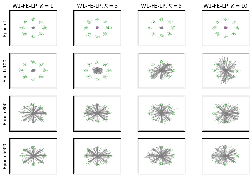
Figure 1: Qualitative evolution of learning process. A sample from the target distribution is given in green, a sample from the initial distribution is in magenta, and the transport rays by the generator are given in the grey arrows. The generate samples lie at the head of each grey arrow.

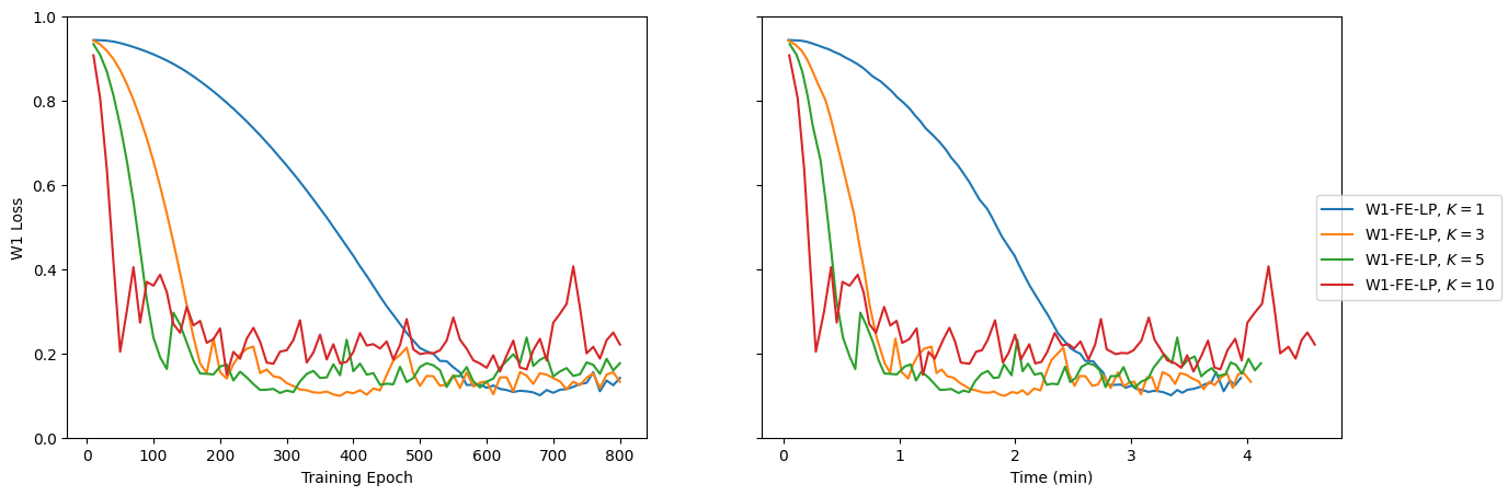
Figure 2: Loss plots of various persistent W1-FE-LP. We specifically plot Wasserstein-$1$ loss against training epoch (left) and wallclock time (right), respectively. Results are shown up to training epoch $800$.

Next, we apply our framework to the unsupervised domain adaptation problem as considered Seguy et al. (2017, Section 5.2). In particular, we use our W1-FE-LP algorithms with varying persistency to solve the domain adaptation problem from the USPS Hull (1994) dataset to the MNIST Deng (2012) dataset. By virtue of Proposition 4.1, we can effectively treat W1-FE-LP with $K=1$ as W1-LP. Hence, we use that as our baseline method. Adaptation performance is evaluated every $100$ training epochs using a $1$-nearest neighbor ($1-$NN) classifier. This is the same performance metric used in Seguy et al. (2017); the difference being that the authors of Seguy et al. (2017) only evaluated their models at the end of training, whereas we evaluate each model throughout training. The results are displayed in Figure 3. From this figure, we can observe that persistent training yields far faster convergence for the algorithms than without it. While it may be too close to be conclusive, we also see that W1-FE-LP with $K=3$ obtains the best overall accuracy, whereas the $K=5$ experiment performed slightly worse. In contrast, the $K=10$ experiment performed the absolute worst among all model tested. This is likely a result of overfitting, where $K=3$ may be a “sweet spot" for the USPS to MNIST adaptation problem. Each experiment had the following shared parameters: $\gamma_{g}=\gamma_{d}=10^{-4}$, the time step is $\epsilon=1$, there were $5$ discriminator updates per training epoch, we used mini batches of size $m=64$ and each experiment was run for $10^{4}$ epochs.

Every experiment was run on the T4 GPU available via Google Colab.

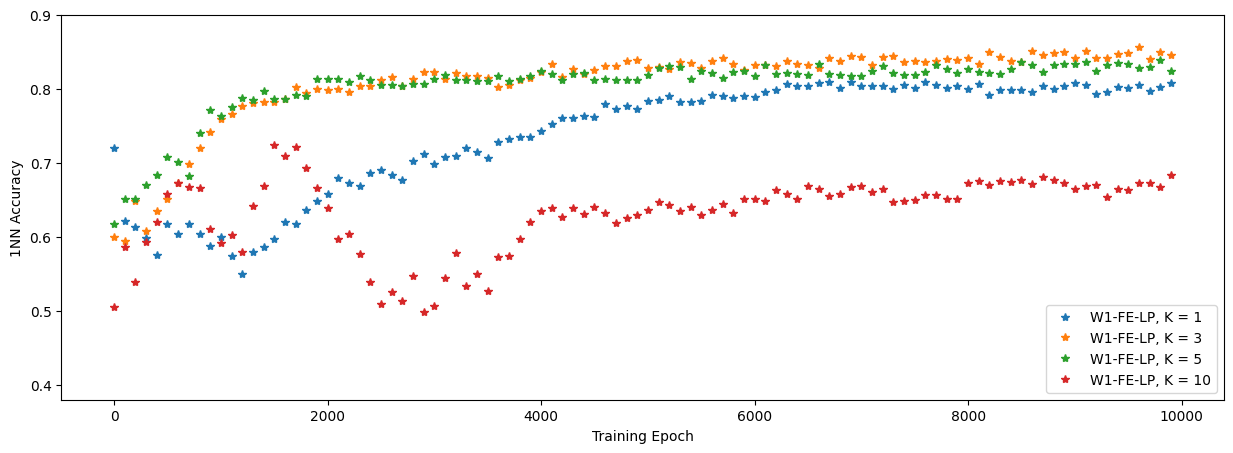
Figure 3: $1$-NN classifier accuracy against training epoch for the USPS to MNIST domain adaptation problem.

6 Limitations

While we have provided many theoretical results, including the crucial convergence result in Theorem 4.1, several theoretical questions remain open. For instance, whether there exists a (unique) solution $Y$ to ODE (3.3) and whether the law of $Y_{t}$ ultimately converges to $\mu_{\operatorname{d}}$ (i.e., $W_{1}(\mu^{Y_{t}},\mu_{\operatorname{d}})\to 0$ as $t\to\infty$) are arguably the most important two questions that remain unanswered. While the theory of gradient flows in $\mathcal{P}_{p}(\mathcal{X})$ for $p>1$ is very well developed (as seen in Ambrosio et al. (2008, Section 11)), the lack of strict convexity in the cost function $|\cdot|$ makes it difficult to obtain analogous results in $\mathcal{P}_{1}(\mathcal{X})$. Furthermore, it is unclear whether $\nabla\varphi_{\mu^{Y_{t}}}^{\mu_{\operatorname{d}}}$ is continuous in $\mathcal{P}_{1}(\mathcal{X})$, making it difficult to apply known results for solving distribution-dependent stochastic differential equations (or, McKean-Vlasov equations).

There are also open questions regarding the discretization (4.1). Perhaps the most crucial one is whether $\mu^{*}(t)=\mu^{Y_{t}}$, where $Y$ is the solution to ODE (3.3); that is, if $\mu_{\epsilon}(t)$ converges to the law of $Y_{t}$ in (3.3). In light of Proposition 4.1, an easier first step could be showing that WGANs converge to the data distribution. However, the authors are currently unaware of any kind of proof for this result.

On the numerical side, we see that persistent training reaps far greater benefits on W1-FE-LP as opposed to W1-FE-GP (see appendix). Given that the ODE update rule relies on the accuracy of the discriminator, we suspect that persistent training is reliable only when the discriminator is accurate enough. This, in turn, limits the variations of W1-FE that can be improved via persistency. Additionally, we see that too much persistency can result in overfitting the data. As such, it is up to the user to be prudent in their choice of persistency. Of course, we only solve a handful of test problems to demonstrate the potential of our algorithms. We believe more numerical experiments are needed in order to fully understand the benefits of our proposed algorithms.

7 Conclusion

By performing “gradient descent” in the space $\mathcal{P}_{1}(\mathcal{X})$, we introduced a distribution-dependent ODE for the purpose of generative modeling. A forward Euler discretization of the ODE converges to a curve of probability measures, suggesting that any numerical implementation of the discretization is stable for small enough time step. This inspired a class of new algorithms (called W1-FE) that naturally involve persistent training. If we (artificially) choose not to implement persistent training, our algorithms simply recover the existing WGAN algorithms. By increasing the level of persistent training suitably (to better simulate the ODE), our algorithms outperform existing WGAN algorithms in numerical examples.

8 Acknowledgements

This project is supported by National Science Foundation under grant DMS-2109002. We also thank Google for their freely available Google Colab, which we used for all simulations.

Appendix A Theoretical results

A.1 A refined Arzelà-Ascoli result, Ambrosio et al. (2008, Proposition 3.3.1)

Proposition A.1.

Let $(\mathfrak{L},d)$ be a complete metric space and let $\sigma$ be a Hausdorff topology on $\mathfrak{L}$ compatible with $d$, that is, weaker than the topology induced by $d$. Furthermore, let $T>0$, let $K\in\mathfrak{L}$ be a sequentially compact set with respect to $\sigma$, and let $g_{n}:[0,T]\rightarrow\mathfrak{L}$ be curves such that

$$g_{n}(t)\in K\quad\forall n\in\mathbb{N},\;t\in[0,T],$$ (A.1)

$$\limsup_{n\rightarrow\infty}d(g_{n}(s),g_{n}(t))\leq\omega(s,t)\quad\forall s,t\in[0,T],$$ (A.2)

for a symmetric function $\omega:[0,T]\times[0,T]\rightarrow[0,+\infty)$, such that

$$\lim_{(s,t)\rightarrow(r,r)}\omega(s,t)=0\quad\forall r\in[0,T]\setminus\mathcal{N},$$ (A.3)

where $\mathcal{N}$ is an (at most) countable subset of $[0,T]$. Then there exists an increasing subsequence $k\rightarrow n(k)$ and a limit curve $g:[0,T]\rightarrow\mathfrak{L}$ such that

$$g_{n(k)}(t)\xrightarrow{\sigma}g(t)\quad\forall t\in[0,T],$$ (A.4)

and $g$ is $d$-continuous in $[0,T]\setminus\mathcal{N}$.

A.2 Proof of Theorem 4.1

Proof.

Our first step is to show that the collection $\{\mu^{Y_{n,\epsilon}}\}$ is tight. To this end, let us observe that the function $\phi(y):=|y|$ for any $y\in\mathbb{R}^{d}$ has compact sublevels. That is, the set

$$\{y:|y|\leq c\}$$ (A.5)

is compact in $\mathbb{R}^{d}$ for any $c\geq 0$, for it is simply the closed ball around $0$ of radius $c$. We observe that for any fixed $t\in[0,T]$ and $\epsilon\in(0,\epsilon_{0})$, there exists $n\in\mathbb{N}$ such that $\mu_{\epsilon}(t)=\mu^{Y_{n-1,\epsilon}}$. Now let us consider the corresponding random variable $Y_{n-1,\epsilon}$, where

$$Y_{n-1,\epsilon}=Y_{0}-\epsilon\sum_{i=0}^{n-2}\nabla\varphi_{\mu^{Y_{i,\epsilon}}}^{\mu_{d}}(Y_{i,\epsilon}).$$ (A.6)

We compute

$$\begin{aligned} \sup_{\epsilon\in(0,\epsilon_{0})}\int_{\mathbb{R}^{d}}|y|\,d\mu_{\epsilon}(t)&=\sup_{\epsilon\in(0,\epsilon_{0})}\int_{\mathbb{R}^{d}}|y|\,d\mu^{Y_{n-1,\epsilon}}\\ &=\sup_{\epsilon\in(0,\epsilon_{0})}\mathbb{E}_{\mathbb{P}}[|Y_{n-1,\epsilon}|]\\ &\leq\sup_{(0,\epsilon_{0})}\mathbb{E}\left[\left|Y_{0}-\epsilon\sum_{i=0}^{n-2}\nabla\varphi_{\mu^{Y_{i,\epsilon}}}^{\mu_{d}}(Y_{i,\epsilon})\right|\right]\\ &\leq\sup_{(0,\epsilon_{0})}\mathbb{E}\left[|Y_{0}|+\epsilon\sum_{i=0}^{n-2}|\nabla\nabla\varphi_{\mu^{Y_{n-1,\epsilon}}}^{\mu_{d}}(Y_{i,\epsilon})|\right]\\ &\leq\sup_{(0,\epsilon_{0})}\mathbb{E}[|Y_{0}|]+(n-1)\epsilon\\ &\leq\mathbb{E}[|Y_{0}|]+T<\infty,\end{aligned}$$ (A.7)

and observe, by Ambrosio et al. (2008, Remark 5.1.5), that this implies that the collection $\{\mu_{\epsilon}(t)\}$ is tight for any $t\in[0,T]$ and $\epsilon\in(0,\epsilon_{0})$. Since $\mathcal{X}\subset\mathbb{R}^{d}$ is compact, (Ambrosio et al., 2008, Remark 7.1.9) implies that this set is precompact in $P_{1}(\mathcal{X})$. Next, we consider two points $s,t\in[0,T]$ and $s\neq t$. Without loss of generality, we take $s<t$. For any fixed $\epsilon\in(0,\epsilon_{0})$, we deduce that there exist $j,k\in\mathbb{N}$ such that

$$\begin{aligned} (j-1)\epsilon<s\leq j\epsilon,&&\\ (k-1)\epsilon<t\leq k\epsilon,&&\end{aligned}$$ (A.8)

and $j\neq k$. Therefore, $\mu_{\epsilon}(s)=\mu^{Y_{j-1,\epsilon}}$ and $\mu_{\epsilon}(t)=\mu^{Y_{k-1,\epsilon}}$, additionally, define $l:=k-j$, we thus have

$$Y_{k-1,\epsilon}=Y_{j-1,\epsilon}-\epsilon\sum_{i=1}^{l}\nabla u_{k-i,\epsilon}(Y_{k-i,\epsilon}).$$ (A.9)

We observe that

$$\begin{aligned} W_{1}(\mu_{\epsilon}(s),\mu_{\epsilon}(t))&=W_{1}(\mu^{Y_{j-1,\epsilon}},\mu^{Y_{k-1,\epsilon}})\\ &\leq\mathbb{E}_{\mathbb{P}}[|Y_{k-1,\epsilon}-Y_{j-1,\epsilon}|]\\ &=\mathbb{E}_{\mathbb{P}}\left[\left|\epsilon\sum_{i=1}^{l}\nabla u_{k-i,\epsilon}(Y_{k-i,\epsilon})\right|\right]\\ &\leq\epsilon l<t-s+\epsilon.\end{aligned}$$ (A.10)

By following the same reasoning but with $s>t$, we observe that

$$W_{1}(\mu_{\epsilon}(s),\mu_{\epsilon}(t))\leq|t-s|+\epsilon.$$ (A.11)

By defining $\omega(s,t):=|s-t|$, which clearly is symmetric and satisfies (A.3), we see that

$$\limsup_{\epsilon\rightarrow 0}W_{1}(\mu_{\epsilon}(s),\mu_{\epsilon}(t))\leq\omega(s,t),\quad\forall s,t\in[0,T].$$ (A.12)

Therefore, we may apply Proposition A.1 to obtain a subsequence $\{\epsilon_{k}\}$ and limiting curve $\mu^{*}(t)$ such that

$$\lim_{k\rightarrow\infty}W_{1}(\mu_{\epsilon_{k}}(t),\mu^{*}(t)),\quad t\in[0,T]\setminus\mathcal{N},$$ (A.13)

for some at most countable subset $\mathcal{N}$ of $[0,T]$. However, since $\omega(s,t)=|s-t|=\mathcal{L}([s,t])$, by Ambrosio et al. (2008, Remark 3.3.2), we conclude that $\mathcal{N}=\emptyset$, for the Lebesgue measure is finite and without atom on the interval $[0,T]$. The conclusions of the theorem thus follow. ∎

Appendix B More Experimental Results

B.1 Persistency on W1-FE-GP

We solved the same two-dimensional problem using W1-FE-GP as that using W1-FE-LP in the main text. The results are shown in Figure 4. As we can see, increasing persistency results in far higher instability for W1-FE-GP as compared to W1-FE-LP. This suggests that an accurate calculation of the Kantorovich potential is essential for improving generator training by increasing persistency.

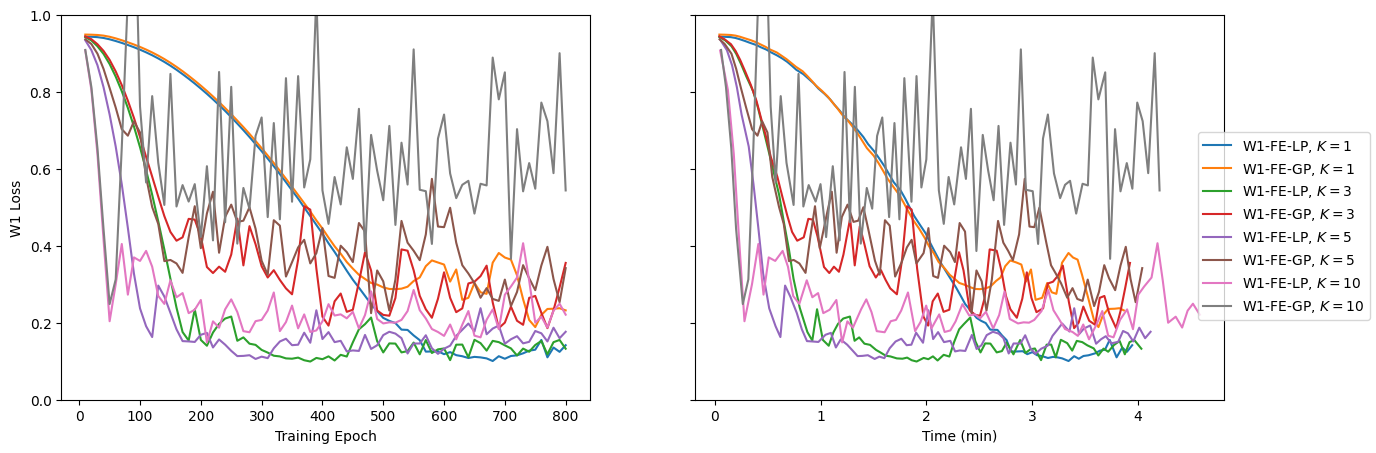
Figure 4: Loss plots of various persistent W1-FE-LP and W1-FE-GP. We specifically plot Wasserstein-$1$ loss against training epoch and wallclock time, respectively. Results are shown up to training epoch $800$.

Appendix C Using the code

We built off of the software package developed for use in Leygonie et al. (2019). While we made substantial changes to the package for our own purposes, we do acknowledge that the package built by Leygonie et al. (2019) made it substantially easier for us to implement our algorithm. The usage is almost identical to the original package’s usage.

We recommend storing the code as either a zipped file or pulling directly from the GitHub repository. We also recommend using a Google Colab notebook as the virtual environment. Once the software package is loaded in the appropriate folder, one may reproduce the low dimensional experiments by running main.py inside exp_2d. The high dimensional experiments may be reproduced by running main.py inside exp_da.

If one uses Google Colab to run the experiments, then the default environment provided by the Google Colab Jupyter notebook in addition to the package Python Optimal Transport (POT) is required to run the software. To reproduce the plots, one needs the package tensorboard.

References

- Ambrosio (2000) L. Ambrosio. Lecture notes on optimal transport problems, 2000. URL http://cvgmt.sns.it/paper/1008/. cvgmt preprint.
- Ambrosio et al. (2008) L. Ambrosio, N. Gigli, and G. Savaré. Gradient flows in metric spaces and in the space of probability measures. Lectures in Mathematics ETH Zürich. Birkhäuser Verlag, Basel, second edition, 2008. ISBN 978-3-7643-8721-1.
- Arjovsky et al. (2017) M. Arjovsky, S. Chintala, and L. Bottou. Wasserstein generative adversarial networks. In D. Precup and Y. W. Teh, editors, Proceedings of the 34th International Conference on Machine Learning, volume 70 of Proceedings of Machine Learning Research, pages 214–223. PMLR, 06–11 Aug 2017. URL https://proceedings.mlr.press/v70/arjovsky17a.html.
- Deng (2012) L. Deng. The mnist database of handwritten digit images for machine learning research. IEEE Signal Processing Magazine, 29(6):141–142, 2012.
- Fischetti et al. (2018) M. Fischetti, I. Mandatelli, and D. Salvagnin. Faster SGD training by minibatch persistency. CoRR, abs/1806.07353, 2018. URL http://arxiv.org/abs/1806.07353.
- Goodfellow et al. (2014) I. J. Goodfellow, J. Pouget-Abadie, M. Mirza, B. Xu, D. Warde-Farley, S. Ozair, A. Courville, and Y. Bengio. Generative adversarial networks, 2014.
- Gulrajani et al. (2017) I. Gulrajani, F. Ahmed, M. Arjokvsky, V. Dumoulin, and A. C. Courville. Improved training of wasserstein gans. Advances in Neural Information Processing Systems, 30, 2017.
- Huang and Zhang (2023) Y. J. Huang and Y. Zhang. Gans as gradient flows that converge. Journal of Machine Learning Research, 24(217):1–40, 2023. URL http://jmlr.org/papers/v24/22-0583.html.
- Hull (1994) J. J. Hull. A database for handwritten text recognition research. IEEE Transactions on Pattern Analysis and Machine Intelligence, 16(5):550–554, 1994. doi: 10.1109/34.291440.
- Jourdain and Tse (2021) B. Jourdain and A. Tse. Central limit theorem over non-linear functionals of empirical measures with applications to the mean-field fluctuation of interacting diffusions. Electron. J. Probab., 26:Paper No. 154, 34, 2021. ISSN 1083-6489. doi: 10.1214/21-ejp720. URL https://doi.org/10.1214/21-ejp720.
- Leygonie et al. (2019) J. Leygonie, J. She, A. Almahairi, S. Rajeswar, and A. C. Courville. Adversarial computation of optimal transport maps. CoRR, abs/1906.09691, 2019. URL http://arxiv.org/abs/1906.09691.
- Metz et al. (2017) L. Metz, B. Poole, D. Pfau, and J. Sohl-Dickstein. Unrolled generative adversarial networks, 2017.
- Petzka et al. (2018) H. Petzka, A. Fischer, and D. Lukovnikov. On the regularization of wasserstein GANs. In International Conference on Learning Representations, 2018. URL https://openreview.net/forum?id=B1hYRMbCW.
- Santambrogio (2015) F. Santambrogio. Optimal transport for applied mathematicians, volume 87 of Progress in Nonlinear Differential Equations and their Applications. Birkhäuser/Springer, Cham, 2015. ISBN 978-3-319-20827-5; 978-3-319-20828-2. doi: 10.1007/978-3-319-20828-2. URL https://doi.org/10.1007/978-3-319-20828-2. Calculus of variations, PDEs, and modeling.
- Seguy et al. (2017) V. Seguy, B. B. Damodaran, R. Flamary, N. Courty, A. Rolet, and M. Blondel. Large-scale optimal transport and mapping estimation, 2017. URL https://arxiv.org/abs/1711.02283.
- Villani (2009) C. Villani. Optimal transport, volume 338 of Grundlehren der mathematischen Wissenschaften [Fundamental Principles of Mathematical Sciences]. Springer-Verlag, Berlin, 2009. ISBN 978-3-540-71049-3. doi: 10.1007/978-3-540-71050-9. URL https://doi.org/10.1007/978-3-540-71050-9. Old and new.