B$\oplus$LD: Boolean Logic Deep Learning

Abstract

Deep learning is computationally intensive, with significant efforts focused on reducing arithmetic complexity, particularly regarding energy consumption dominated by data movement. While existing literature emphasizes inference, training is considerably more resource-intensive. This paper proposes a novel mathematical principle by introducing the notion of Boolean variation such that neurons made of Boolean weights and inputs can be trained —for the first time— efficiently in Boolean domain using Boolean logic instead of gradient descent and real arithmetic. We explore its convergence, conduct extensively experimental benchmarking, and provide consistent complexity evaluation by considering chip architecture, memory hierarchy, dataflow, and arithmetic precision. Our approach achieves baseline full-precision accuracy in ImageNet classification and surpasses state-of-the-art results in semantic segmentation, with notable performance in image super-resolution, and natural language understanding with transformer-based models. Moreover, it significantly reduces energy consumption during both training and inference.

1 Introduction

Deep learning [58] has become the de facto solution to a wide range of tasks. However, running deep learning models for inference demands significant computational resources, yet it is just the tip of the iceberg. Training deep models is even much more intense. The extensive literature on this issue can be summarized into four approaches addressing different sources of complexity. These include: (1) model compression, pruning [38, 20, 104] and network design [90, 44, 92] for large model dimensions; (2) arithmetic approximation [57, 90, 15] for intensive multiplication; (3) quantization techniques like post-training [101, 34], quantization-aware training [37, 109, 51], and quantized training to reduce precision [16, 89]; and (4) hardware design [18, 83, 100, 97, 35, 107] to overcome computing bottleneck by moving computation closer to or in memory.

Aside from hardware and dataflow design, deep learning designs have primarily focused on the number of compute operations (ops), such as flops or bops, as a complexity measure [33, 79] rather than the consumed energy or memory, and particularly in inference tasks. However, it has been demonstrated that ops alone are inadequate and even detrimental as a measure of system complexity. Instead, energy consumption provides a more consistent and efficient metric for computing hardware [90, 91, 103, 88]. Data movement, especially, dominates energy consumption and is closely linked to system architecture, memory hierarchy, and dataflow [56, 85, 105, 19]. Therefore, efforts aimed solely at reducing ops are inefficient.

Quantization-aware training, notably binarized neural networks (bnns) [24, 47], have garnered significant investigation [see, e.g. 79, 34, and references therein]. bnns typically binarize weights and activations, forming principal computation blocks in binary. They learn binary weights, $\mathbf{w}_{\texttt{bin}}$, through full-precision (fp) latent weights, $\mathbf{w}_{\texttt{fp}}$, leading to no memory or computation savings during training. For example, a binarized linear layer is operated as $s=\alpha\cdot\mathbf{w}_{\texttt{bin}}^{\top}\mathbf{x}_{\texttt{bin}}$, where $s$ is the output and $\alpha$ is a fp scaling factor, $\mathbf{w}_{\texttt{bin}}=\operatorname{sign}(\mathbf{w}_{\texttt{fp}})$, and $\mathbf{x}_{\texttt{bin}}=\operatorname{sign}(\mathbf{x}_{\texttt{fp}})$ is the binarized inputs. The weights are updated via common gradient descent backpropagation, i.e. $\mathbf{w}_{\texttt{bin}}=\operatorname{sign}(\mathbf{w}_{\texttt{fp}}-\eta\cdot\mathbf{g}_{\mathbf{w}_{\texttt{fp}}})$ with a learning rate $\eta$, and fp gradient signal $\mathbf{g}_{\mathbf{w}_{\texttt{fp}}}$. Gradient approximation of binarized variables often employs a differentiable proxy of the binarization function $\operatorname{sign}$, commonly the identity proxy. Various approaches treat bnn training as a constrained optimization problem [6, 2, 3, 64], exploring methods to derive binary weights from real-valued latent ones. bnns commonly suffers notable accuracy drops due to reduced network capacity and the use of proxy fp optimizers [60] instead of operating directly in binary domain [79, 75, 36]. Recent works mitigate this by incorporating multiple fp components in the network, retaining only a few binary dataflows [67]. Thus, while binarization aids in reducing inference complexity, it increases network training complexity and memory usage.

In contrast to binarizing fp models like bnns, designing native binary models not relying on fp latent weight has been explored. For example, Expectation Backpropagation [87], although operating on full-precision training, was proposed for this purpose. Statistical physics-inspired [7, 8] and Belief Propagation [9] algorithms utilize integer latent weights, mainly applied to single perceptrons, with unclear applicability to deep models. Evolutionary algorithms [74, 50] are also an alternative but encounter performance and scalability challenges.

• We introduce the notion of variation to the Boolean logic and develop a new mathematical framework of function variation (see § 3.2). One of the noticeable properties is that Boolean variation has the chain rule (see Theorem 3.11) similar to the continuous gradient.

• Based on the proposed framework, we develop a novel Boolean backpropagation and optimization method allowing for a deep model to support native Boolean components operated solely with Boolean logic and trained directly in Boolean domain, eliminating the need for gradient descent and fp latent weights (see § 3.3). This drastically cuts down memory footprint and energy consumption during both training and inference (see, e.g., Fig. 1).

• We provide a theoretical analysis of the convergence of our training algorithm (see Theorem 3.16).

• We conduct an extensive experimental campaign using modern network architectures such as convolutional neural networks (cnns) and Transformers [96] on a wide range of challenging tasks including image classification, segmentation, super-resolution and natural language understanding (see § 4). We rigorously evaluate analytically the complexity of b$\oplus$ld and bnns. We demonstrate the superior performance of our method in terms of both accuracy and complexity compared to the state-of-the-art (see, e.g., Table 6, Table 6, Table 7).

2 Are Current Binarized Neural Networks Really Efficient?

Our work is closely related with the line of research on binarized neural networks (bnns). The concept of bnns traces back to early efforts to reduce the complexity of deep learning models. binaryconnect [24] is one of the pioneering works that introduced the idea of binarizing fp weights during training, effectively reducing memory footprint and computational cost. Similarly, binarynet [47], xnor-net [82] extended this approach to binarize both weights and activations, further enhancing the efficiency of neural network inference. However, these early bnns struggled with maintaining accuracy comparable to their full-precision counterparts. To address this issue, significant advances have been made on bnns [see, e.g., 79, 81, and references therein], which can be categorized into three main aspects.

\raisebox{-.9pt} {{\small{1}}}⃝ Binarization strategy.

The binarization strategy aims to efficiently convert real-valued data such as activations and weights into binary form $\{-1,1\}$. The $\operatorname{sign}$ function is commonly used for this purpose, sometimes with additional constraints such as clipping bounds in state-of-the-art (sota) methods like pokebnn [112] or bnext [36]. reactnet [67] introduces $\operatorname{rsign}$ as a more general alternative to the $\operatorname{sign}$ function, addressing potential shifts in the distribution of activations and weights. Another approach [95] explores the use of other two real values instead of strict binary to enhance the representational capability of bnns.

\raisebox{-.9pt} {{\small{2}}}⃝ Optimization and training strategy.

bnn optimization relies totally on latent-weight training, necessitating a differentiable proxy for the backpropagation. Moreover, latent-weight based training methods have to store binary and real parameters during training and often requires multiple sequential training stages, where one starts with training a fp model and only later enables binarization [36, 112, 102]. This further increases the training costs. Furthermore, knowledge distillation (kd) has emerged as a method to narrow the performance gap by transferring knowledge from a full-precision teacher model to a binary model [67, 102, 112, 59]. While a single teacher model can sufficiently improve the accuracy of the student model, recent advancements like multi-kd with multiple teachers, such as bnext [36], have achieved unprecedented performance. However, the kd approach often treats network binarization as an add-on to full-precision models. In addition, this training approach relies on specialized teachers for specific tasks, limiting adaptability on new data. Lastly, [99, 41] proposed some heuristics and improvements to the classic bnn latent-weight based optimizer.

Figure 1: Comparisons of our method against notable bnns on cifar10 with vgg-small, evaluated on Nvidia Tesla V100.

Table 1: A summary of sota bnns compared to our method. The notation ✗ indicates the nonexistence of a specific requirement (column) within a given method (row). The colors denoting the methods shall be used consistently throughout the paper.

Method	Bitwidth	Specialized	Mandatory	Multi-stage or	Weight	Backprop	Training
	(Weight-Act.)	Architecture	FP Components	KD Training	Updates		Arithmetic
( ) binarynet [47]	1-1	✗	✗	✗	FP latent-weights	Gradient	FP
( ) binaryconnect [24]	1-32	✗	✗	✗	FP latent-weights	Gradient	FP
( ) xnor-net [82]	1-1	✗	✗	✗	FP latent-weights	Gradient	FP
( ) bi-realnet [68]	1-1	✓	✓	✓	FP latent-weights	Gradient	FP
( ) real2binary [72]	1-1	✓	✓	✓	FP latent-weights	Gradient	FP
( ) reactnet [67]	1-1	✓	✓	✓	FP latent-weights	Gradient	FP
( ) melius-net [10]	1-1	✓	✓	✓	FP latent-weights	Gradient	FP
( ) bnext [36]	1-1	✓	✓	✓	FP latent-weights	Gradient	FP
( ) pokebnn [112]	1-1	✓	✓	✓	FP latent-weights	Gradient	FP
( ) b$\oplus$ld [Ours]	1-1	✗	✗	✗	Native Boolean weights	Logic	Logic

\raisebox{-.9pt} {{\small{3}}}⃝ Architecture design.

Architecture design in bnns commonly utilizes resnet [68, 67, 10, 36] and mobilenet [67, 36] layouts. These methodologies often rely on heavily modified basic blocks, including additional shortcuts, automatic channel scaling via squeeze-and-excitation (se) [112], block duplication with concatenation in the channel domain [67, 36]. Recent approaches introduce initial modules to enhance input adaptation for binary dataflow [102] or replace convolutions with lighter point-wise convolutions [65].

Summary.

Table 1 shows key characteristics of sota bnn methods. These methods will be considered in our experiments. Notice that all these techniques indeed have to involve operations on fp latent weights during training, whereas our proposed method works directly on native Boolean weights. In addition, most of bnn methods incorporate fp data and modules as mandatory components. As a result, existing bnns consume much more training energy compared to our b$\oplus$ld method. An example is shown in Fig. 1, where we consider the vgg-small architecture [86] on cifar10 dataset. In § 4 we will consider much larger datasets and networks on more challenging tasks. We can see that our method achieves $36\times$ and more than $15\times$ energy reduction compared to the fp baseline and binarynet, respectively, while yielding better accuracy than bnns. Furthermore, bnns are commonly tied to specialized network architecture and have to employ costly multi-stage or kd training. Meanwhile, our Boolean framework is completely orthogonal to these bnn methods. It is generic and applicable for a wide range of network architectures, and its training procedure purely relies on Boolean logic from scratch. Nevertheless, we stress that it is not obligatory to use all Boolean components in our proposed framework as it is flexible and can be extended to architectures comprised of a mix of Boolean and fp modules. This feature further improves the superior performance of our method as can be seen in Fig. 1, where we integrate batch normalization (bn) [49] into our Boolean model, and we will demonstrate extensively in our experiments.

3 Proposed Method

3.1 Neuron Design

Boolean Neuron.

For the sake of simplicity, we consider a linear layer for presenting the design. Let $w_{0}$, $(w_{1},\ldots,w_{m})$, and $(x_{1},\ldots,x_{m})$ be the bias, weights, and inputs of a neuron of input size $m\geq 1$. In the core use case of our interest, these variables are all Boolean numbers. Let $\mathrm{L}$ be a logic gate such as and, or, xor, xnor. The neuron’s pre-activation output is given as follows:

$$s=w_{0}+\sum_{i=1}^{m}\mathrm{L}(w_{i},x_{i}),$$ (1)

where the summation is understood as the counting of trues.

Mixed Boolean-Real Neuron.

To allow for flexible use and co-existence of this Boolean design with real-valued parts of a deep model, two cases of mixed-type data are considered including Boolean weights with real-valued inputs, and real-valued weights with Boolean inputs. These two cases can be addressed by the following extension of Boolean logic to mixed-type data. To this end, we first introduce the essential notations and definitions. Specifically, we denote $\mathbb{B}:=\{\mathrm{T},\mathrm{F}\}$ equipped with the Boolean logic. Here, $\mathrm{T}$ and $\mathrm{F}$ indicate true and false, respectively.

Definition 3.1 (Three-valued logic).

Define $\mathbb{M}\operatorname*{\overset{{\rm def}}{=}}\mathbb{B}\cup\{0\}$ with logic connectives defined according to those of Boolean logic as follows. First, the negation is: $\neg\mathrm{T}=\mathrm{F}$, $\neg\mathrm{F}=\mathrm{T}$, and $\neg 0=0$. Second, let $\mathrm{L}$ be a logic connective, denote by $\mathrm{L}_{\mathbb{M}}$ and $\mathrm{L}_{\mathbb{B}}$ when it is in $\mathbb{M}$ and in $\mathbb{B}$, respectively, then $\mathrm{L}_{\mathbb{M}}(a,b)=\mathrm{L}_{\mathbb{B}}(a,b)$ for $a,b\in\mathbb{B}$ and $\mathrm{L}_{\mathbb{M}}(a,b)=0$ otherwise.

Notation 3.2.

Denote by $\mathbb{L}$ a logic set (e.g., $\mathbb{B}$ or $\mathbb{M}$), $\mathbb{R}$ the real set, $\mathbb{Z}$ the set of integers, $\mathbb{N}$ a numeric set (e.g., $\mathbb{R}$ or $\mathbb{Z}$), and $\mathbb{D}$ a certain set of $\mathbb{L}$ or $\mathbb{N}$.

Definition 3.3.

For $x\in\mathbb{N}$, its logic value denoted by $x_{\mathrm{logic}}$ is given as $x_{\mathrm{logic}}=\mathrm{T}\Leftrightarrow x>0$, $x_{\mathrm{logic}}=\mathrm{F}\Leftrightarrow x<0$, and $x_{\mathrm{logic}}=0\Leftrightarrow x=0$.

Definition 3.4.

The magnitude of a variable $x$, denoted $|x|$, is defined as its usual absolute value if $x\in\mathbb{N}$. And for $x\in\mathbb{L}$: $|x|=0$ if $x=0$, and $|x|=1$ otherwise.

Definition 3.5 (Mixed-type logic).

For $\mathrm{L}$ a logic connective of $\mathbb{L}$ and variables $a$, $b$, operation $c=\mathrm{L}(a,b)$ is defined such that $|c|=|a||b|$ and $c_{\mathrm{logic}}=\mathrm{L}(a_{\mathrm{logic}},b_{\mathrm{logic}})$.

Using Definition 3.5, neuron formulation Eq. 1 directly applies to the mixed Boolean-real neurons.

Forward Activation.

It is clear that there can be only a unique family of binary activation functions that is the threshold one. Let $\tau$ be a scalar, which can be fixed or learned, the forward Boolean activation is given as follows: $y=\mathrm{T}$ if $s\geq\tau$ and $y=\mathrm{F}$ if $s<\tau$ where $s$ is the preactivation.

3.2 Mathematical Foundation

In this section we describe the mathematical foundation for our method to train Boolean weights directly in the Boolean domain without relying on fp latent weights. Due to the space limitation, essential notions necessary for presenting the main results are presented here while a comprehensive treatment is provided in Appendix A.

Definition 3.6.

Order relations ‘$<$’ and ‘$>$’ in $\mathbb{B}$ are defined as follows: $\mathrm{F}<\mathrm{T}$, and $\mathrm{T}>\mathrm{F}$.

Definition 3.7.

For $a,b\in\mathbb{B}$, the variation from $a$ to $b$, denoted $\delta(a\to b)$, is defined as: $\delta(a\to b)\operatorname*{\overset{{\rm def}}{=}}\mathrm{T}$ if $b>a$, $\operatorname*{\overset{{\rm def}}{=}}0$ if $b=a$, and $\operatorname*{\overset{{\rm def}}{=}}\mathrm{F}$ if $b<a$.

Definition 3.8.

For $f\in\mathcal{F}(\mathbb{B},\mathbb{D})$, $\forall x\in\mathbb{B}$, write $\delta f(x\to\neg x):=\delta(f(x)\to f(\neg x))$. The variation of $f$ w.r.t. $x$, denoted $f^{\prime}(x)$, is defined as: $f^{\prime}(x)\operatorname*{\overset{{\rm def}}{=}}\mathbf{xnor}(\delta(x\to\neg x),\delta f(x\to\neg x))$.

Intuitively, the variation of $f$ w.r.t. $x$ is $\mathrm{T}$ if $f$ varies in the same direction with $x$.

Example 3.9.

Let $a\in\mathbb{B}$, $f(x)=\mathbf{xor}(x,a)$ for $x\in\mathbb{B}$, the variation of $f$ w.r.t. $x$ can be derived by establishing a truth table (see Table 8 in § A.1) from which we obtain $f^{\prime}(x)=\neg a$.

For $f\in\mathcal{F}(\mathbb{Z},\mathbb{N})$, its derivative has been defined in the literature as $f^{\prime}(x)=f(x+1)-f(x)$. With the logic variation as introduced above, we can make this definition more generic as follows.

Definition 3.10.

For $f\in\mathcal{F}(\mathbb{Z},\mathbb{D})$, the variation of $f$ w.r.t. $x\in\mathbb{Z}$ is defined as $f^{\prime}(x)\operatorname*{\overset{{\rm def}}{=}}\delta f(x\to x+1)$, where $\delta f$ is in the sense of the variation defined in $\mathbb{D}$.

Theorem 3.11.

The following properties hold:

1. For $f\in\mathcal{F}(\mathbb{B},\mathbb{B})$: $(\neg f)^{\prime}(x)=\neg f^{\prime}(x)$, $\forall x\in\mathbb{B}$.

2. For $f\in\mathcal{F}(\mathbb{B},\mathbb{N})$, $\alpha\in\mathbb{N}$: $(\alpha f)^{\prime}(x)=\alpha f^{\prime}(x)$, $\forall x\in\mathbb{B}$.

3. For $f,g\in\mathcal{F}(\mathbb{B},\mathbb{N})$: $(f+g)^{\prime}(x)=f^{\prime}(x)+g^{\prime}(x)$, $\forall x\in\mathbb{B}$.

4. For $\mathbb{B}\overset{f}{\to}\mathbb{B}\overset{g}{\to}\mathbb{D}$: $(g\circ f)^{\prime}(x)=\mathbf{xnor}(g^{\prime}(f(x)),f^{\prime}(x))$, $\forall x\in\mathbb{B}$.

5. For $\mathbb{B}\overset{f}{\to}\mathbb{Z}\overset{g}{\to}\mathbb{D}$, $x\in\mathbb{B}$, if $|f^{\prime}(x)|\leq 1$ and $g^{\prime}(f(x))=g^{\prime}(f(x)-1)$, then:

   $$(g\circ f)^{\prime}(x)=\mathbf{xnor}(g^{\prime}(f(x)),f^{\prime}(x)).$$

The proof is provided in § A.1. These results are extended to the multivariate case in a straightforward manner. For instance, for multivariate Boolean functions it is as follows.

Definition 3.12.

For $\mathbf{x}=(x_{1},\ldots,x_{n})\in\mathbb{B}^{n}$, denote $\mathbf{x}_{\neg i}:=(x_{1},\ldots,x_{i-1},\neg x_{i},x_{i+1},\ldots,x_{n})$ for $n\geq 1$ and $1\leq i\leq n$. For $f\in\mathcal{F}(\mathbb{B}^{n},\mathbb{B})$, the (partial) variation of $f$ w.r.t. $x_{i}$, denoted $f^{\prime}_{i}(\mathbf{x})$ or $\delta f(\mathbf{x})/\delta x_{i}$, is defined as: $f^{\prime}_{i}(\mathbf{x})\equiv\delta f(\mathbf{x})/\delta x_{i}\operatorname*{\overset{{\rm def}}{=}}\mathbf{xnor}(\delta(x_{i}\to\neg x_{i}),\delta f(\mathbf{x}\to\mathbf{x}_{\neg i}))$.

Proposition 3.13.

Let $f\in\mathcal{F}(\mathbb{B}^{n},\mathbb{B})$, $n\geq 1$, and $g\in\mathcal{F}(\mathbb{B},\mathbb{B})$. For $1\leq i\leq n$:

$$(g\circ f)^{\prime}_{i}(\mathbf{x})=\mathbf{xnor}(g^{\prime}(f(\mathbf{x})),f^{\prime}_{i}(\mathbf{x})),\quad\forall\mathbf{x}\in\mathbb{B}^{n}.$$ (2)

Example 3.14.

From Example 3.9, we have $\delta\mathbf{xor}(x,a)/\delta x=\neg a$ for $a,x\in\mathbb{B}$. Using Theorem 3.11-(1) we have: $\delta\mathbf{xnor}(x,a)/\delta x=a$ since $\mathbf{xnor}(x,a)=\neg\mathbf{xor}(x,a)$.

Example 3.15.

Apply Theorem 3.11-(3) to $s$ from Eq. 1: $\delta s/\delta w_{i}=\delta\mathrm{L}(w_{i},x_{i})/\delta w_{i}$ and $\delta s/\delta x_{i}=\delta\mathrm{L}(w_{i},x_{i})/\delta x_{i}$. Then, for $\mathrm{L}=\mathbf{xnor}$ as an example, we have: $\delta s/\delta w_{i}=x_{i}$ and $\delta s/\delta x_{i}=w_{i}$.

3.3 BackPropagation

With the notions introduced in § 3.2, we can write signals involved in the backpropagation process as shown in Fig. 2. Therein, layer $l$ is a Boolean layer of consideration. For the sake of presentation simplicity, layer $l$ is assumed a fully-connected layer, and:

$$x_{k,j}^{l+1}=w_{0,j}^{l}+\sum_{i=1}^{m}\mathrm{L}\left(x_{k,i}^{l},w_{i,j}^{l}\right),\quad 1\leq j\leq n,$$ (3)

where $\mathrm{L}$ is the utilized Boolean logic, $k$ denotes sample index in the batch, $m$ and $n$ are the usual layer input and output sizes. Layer $l$ is connected to layer $l+1$ that can be an activation layer, a batch normalization, an arithmetic layer, or any others. The nature of $\delta\mathrm{Loss}/\delta x_{k,j}^{l+1}$ depends on the property of layer $l+1$. It can be the usual gradient if layer $l+1$ is a real-valued input layer, or a Boolean variation if layer $l+1$ is a Boolean-input layer. Given $\delta\mathrm{Loss}/\delta x_{k,j}^{l+1}$, layer $l$ needs to optimize its Boolean weights and compute signal $\delta\mathrm{Loss}/\delta x_{k,i}^{l}$ for the upstream. Hereafter, we consider $\mathrm{L}=\mathbf{xnor}$ when showing concrete illustrations of the method.

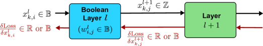
Figure 2: Illustration of backpropagation signals with a Boolean linear layer. Notice that the subsequent layer can be any fp/Boolean layers or activation functions.

Atomic Variation.

First, using Theorem 3.11 and its extension to the multivariate case by Proposition 3.13 in the same manner as shown in Example 3.15, we have:

$$\frac{\delta x_{k,j}^{l+1}}{\delta w_{i,j}^{l}}=\frac{\delta\mathrm{L}(x_{k,i}^{l},w_{i,j}^{l})}{\delta w_{i,j}^{l}}\overset{\mathbf{xnor}}{=}x_{k,i}^{l},\quad\frac{\delta x_{k,j}^{l+1}}{\delta x_{k,i}^{l}}=\frac{\delta\mathrm{L}(x_{k,i}^{l},w_{i,j}^{l})}{\delta x_{k,i}^{l}}\overset{\mathbf{xnor}}{=}w_{i,j}^{l}.$$ (4)

Using the chain rules given by Theorem 3.11–(4 & 5), we have:

$$q_{i,j,k}^{l}:=\frac{\delta\mathrm{Loss}}{\delta w_{i,j}^{l}}|_{k} =\mathbf{xnor}(\frac{\delta\mathrm{Loss}}{\delta x_{k,j}^{l+1}},\frac{\delta x_{k,j}^{l+1}}{\delta w_{i,j}^{l}})\overset{\mathbf{xnor}}{=}\mathbf{xnor}(\frac{\delta\mathrm{Loss}}{\delta x_{k,j}^{l+1}},x_{k,i}^{l}),$$ (5)

$$g_{k,i,j}^{l}:=\frac{\delta\mathrm{Loss}}{\delta x_{k,i}^{l}}|_{j} =\mathbf{xnor}(\frac{\delta\mathrm{Loss}}{\delta x_{k,j}^{l+1}},\frac{\delta x_{k,j}^{l+1}}{\delta x_{k,i}^{l}})\overset{\mathbf{xnor}}{=}\mathbf{xnor}(\frac{\delta\mathrm{Loss}}{\delta x_{k,j}^{l+1}},w_{i,j}^{l}).$$ (6)

Aggregation.

Atomic variation $q_{i,j,k}^{l}$ is aggregated over batch dimension $k$ while $g_{k,i,j}^{l}$ is aggregated over output dimension $j$. Let $\mathbf{1}\left(\cdot\right)$ be the indicator function. For $b\in\mathbb{B}$ and variable $x$, define: $\mathbf{1}\left(x=b\right)=1$ if $x_{\mathrm{logic}}=b$ and $\mathbf{1}\left(x=b\right)=0$ otherwise. Atomic variations are aggregated as:

$$q_{i,j}^{l}:=\frac{\delta\mathrm{Loss}}{\delta w_{i,j}^{l}} =\sum_{k}\mathbf{1}\left(q_{i,j,k}^{l}=\mathrm{T}\right)|q_{i,j,k}^{l}|-\sum_{k}\mathbf{1}\left(q_{i,j,k}^{l}=\mathrm{F}\right)|q_{i,j,k}^{l}|,$$ (7)

$$g_{k,i}^{l}:=\frac{\delta\mathrm{Loss}}{\delta x_{k,i}^{l}} =\sum_{j}\mathbf{1}\left(g_{k,i,j}^{l}=\mathrm{T}\right)|g_{k,i,j}^{l}|-\sum_{j}\mathbf{1}\left(g_{k,i,j}^{l}=\mathrm{F}\right)|g_{k,i,j}^{l}|.$$ (8)

Boolean Optimizer.

With $q_{i,j}^{l}$ obtained in Eq. 7, the rule for optimizing $w_{i,j}^{l}$ subjected to making the loss decreased is simply given according to its definition as:

$$\boxed{w_{i,j}^{l}=\neg w_{i,j}^{l}\textrm{ if }\mathbf{xnor}\left(q_{i,j}^{l},w_{i,j}^{l}\right)=\mathrm{T}.}$$ (9)

Eq. 9 is the core optimization logic based on which more sophisticated forms of optimizer can be developed in the same manner as different methods such as Adam, Adaptive Adam, etc. have been developed from the basic gradient descent principle. For instance, the following is an optimizer that accumulates $q_{i,j}^{l}$ over training iterations. Denote by $q_{i,j}^{l,t}$ the optimization signal at iteration $t$, and by $m_{i,j}^{l,t}$ its accumulator with $m_{i,j}^{l,0}:=0$ and:

$$m_{i,j}^{l,t+1}=\beta^{t}m_{i,j}^{l,t}+\eta^{t}q_{i,j}^{l,t+1},$$ (10)

where $\eta^{t}$ is an accumulation factor that can be tuned as a hyper-parameter, and $\beta^{t}$ is an auto-regularizing factor that expresses the system’s state at time $t$. Its usage is linked to brain plasticity [31] and Hebbian theory [40] forcing weights to adapt to their neighborhood. For the chosen weight’s neighborhood, for instance, neuron, layer, or network level, $\beta^{t}$ is given as:

$$\beta^{t}=\frac{\textrm{Number of unchanged weights at }t}{\textrm{Total number of weights}}.$$ (11)

In the experiments presented later, $\beta^{t}$ is set to per-layer basis. Finally, the learning process is as described in Algorithm 1. We encourage the readers to check the detailed implementations, practical considerations, and example codes of our proposed method, available in Appendix B and Appendix C.

Input :  Learning rate $\eta$, nb iterations $T$;

Initialize :  $m_{i,j}^{l,0}=0$; $\beta^{0}=1$;

1 for $t=0,\dots,T-1$ do

       /* 1. Forward */

2       Compute $x^{l+1,t}$ following Eq. 3;

       /* 2. Backward */

3       Receive $\frac{\delta\mathrm{Loss}}{\delta x_{k,j}^{l+1,t}}$ from downstream layer;

       /* 2.1 Backpropagation */

4       Compute and backpropagate $g^{l,t}$ of Eq. 8;

       /* 2.2 Weight update process */

5       $N_{\textrm{tot}}:=0$, $N_{\textrm{unchanged}}:=0$;

6       foreach $w_{i,j}^{l}$ do

7             Compute $q_{i,j}^{l,t+1}$ following Eq. 7;

8             Update $m_{i,j}^{l,t+1}=\beta^{t}m_{i,j}^{l,t}+\eta^{t}q_{i,j}^{l,t+1}$;

9             $N_{\textrm{tot}}\leftarrow N_{\textrm{tot}}+1$;

10             if $\mathbf{xnor}(m_{i,j}^{l,t+1},w_{i,j}^{l,t})=\mathrm{T}$ then

                   $w_{i,j}^{l,t+1}=\neg w_{i,j}^{l,t}$ ;

                    /* invert */

11                   $m_{i,j}^{l,t+1}=0$;

12                  

13            else

                   $w_{i,j}^{l,t+1}=w_{i,j}^{l,t}$ ;

                    /* keep */

14                   $N_{\textrm{unchanged}}\leftarrow N_{\textrm{unchanged}}+1$;

15                  

16             end if

17            

18       end foreach

19      Update $\eta^{t+1}$, $\beta^{t+1}=N_{\textrm{unchanged}}/N_{\textrm{tot}}$ ;

20      

21 end for

Algorithm 1 Illustration with a FC layer.

Convergence Analysis.

The following result describes how the iterative logic optimization based on Eq. 9 minimizes a predefined loss $f$, under the standard non-convex assumption. The technical assumptions and the proof are given in § A.2.

Theorem 3.16.

Under the specified assumptions, Boolean optimization logic converges at:

$$\frac{1}{T}\sum_{t=0}^{T-1}\mathbb{E}\left[\left\|\nabla f\left(w_{t}\right)\right\|^{2}\right]\leq\frac{A^{*}}{T\eta}+B^{*}\eta+C^{*}\eta^{2}+Lr_{d},$$ (12)

where $A^{*}={2(f(w_{0})-f_{*})}$ with $f_{*}$ being uniform lower bound assumed exists, $B^{*}=2L\sigma^{2}$, $C^{*}=4L^{2}\sigma^{2}\frac{\gamma}{(1-\gamma)^{2}}$ in which $L$ is the assumed Lipschitz constant, and $r_{d}=\nicefrac{{d\kappa}}{{2}}$.

The bound in Theorem 3.16 contains four terms. The first is typical for a general non-convex target and expresses how initialization affects the convergence. The second and third terms depend on the fluctuation of the minibatch gradients. There is an “error bound” of $2Ld\kappa$ independent of $T$. This error bound is the cost of using discrete weights as part of the optimization algorithm. Previous work with quantized models also includes such error bounds [60, 61].

4 Experiments

Our b$\oplus$ld method achieves extreme compression by using both Boolean activations and weights. We rigorously evaluate its performance on challenging precision-demanding tasks, including image classification on cifar10 [54] and imagenet [55], as well as super-resolution on five popular datasets. Furthermore, recognizing the necessity of deploying efficient lightweight models for edge computing, we delve into three fine-tuning scenarios, showcasing the adaptability of our approach. Specifically, we investigate fine-tuning Boolean models for image classification on cifar10 and cifar100 using vgg-small. For segmentation tasks, we study deeplabv3 [17] fine-tuned on cityscapes [23] and pascal voc 2012 [29] datasets. The backbone for such a model is our Boolean resnet18 [39] network trained from scratch on imagenet. Finally, we consider an evaluation in the domain of natural language understanding, fine-tuning bert [26], a transformer-based [96] language model, on the glue benchmark [98].

Experimental Setup.

To construct our b$\oplus$ld models, we introduce Boolean weights and activations and substitute full-precision (fp) arithmetic layers with Boolean equivalents. Throughout all benchmarks, we maintain the general network design of the chosen fp baseline, while excluding fp-specific components like ReLU, PReLU activations, or batch normalization (bn) [49], unless specified otherwise. Consistent with the common setup in existing literature [see, e.g., 82, 21, 10], only the first and last layers remain in fp and are optimized using an Adam optimizer [53]. Comprehensive experiment details for reproducibility are provided in Appendix D.

Complexity Evaluation.

It has been demonstrated that relying solely on flops and bops for complexity assessment is inadequate [90, 91, 103, 88]. In fact, these metrics fail to capture the actual load caused by propagating fp data through the bnns. Instead, energy consumption serves as a crucial indicator of efficiency. Given the absence of native Boolean accelerators, we estimate analytically energy consumption by analyzing the arithmetic operations, data movements within storage/processing units, and the energy cost of each operation. This approach is implemented for the Nvidia GPU (Tesla V100) and Ascend [62] architectures. Further details are available in Appendix E.

4.1 Image Classification

Our b$\oplus$ld method is tested on two network configurations: small & compact and large & deep. In the former scenario, we utilize the vgg-small [86] baseline trained on cifar10. Evaluation of our Boolean architecture is conducted both without bn [24], and with bn including activation from [68]. These designs achieve $90.29\small{\pm 0.09}$% (estimated over six repetitions) and $92.37\small{\pm 0.01}$% (estimated over five repetitions) accuracy, respectively (see Table 6). Notably, without bn, our results align closely with binaryconnect [24], which employs $32$-bit activations during both inference and training. Furthermore, bn brings the accuracy within $1$ point of the fp baseline.

Our method requires much less energy than the fp baseline. In particular, it consumes less than 5% of energy for our designs with and without bn respectively. These results highlight the remarkable energy efficiency of our b$\oplus$ld method in both inference and training, surpassing latent-weight based training methods [24, 82, 48] reliant on fp weights. Notably, despite a slight increase in energy consumption, utilizing bn yields superior accuracy. Even with bn, our approach maintains superior efficiency compared to alternative methods, further emphasizing the flexibility of our approach in training networks with a blend of Boolean and fp components.

In the large & deep case, we consider the resnet18 baseline trained from scratch on imagenet. We compare our approach to methods employing the same baseline, larger architectures, and additional training strategies such as kd with a resnet34 teacher or fp-based shortcuts [68]. Our method consistently achieves the highest accuracy across all categories, ranging from the standard model ($51.8$% accuracy) to larger configurations ($70.0$% accuracy), as shown in Table 6. Additionally, our b$\oplus$ld method exhibits the smallest energy consumption in most categories, with a remarkable $24.45\%$ for our large architecture with and without kd. Notably, our method outperforms the fp baseline when using $4\times$ filter enlargement (base 256), providing significant energy reduction ($24.45\%$). Furthermore, it surpasses the sota pokebnn [112], utilizing resnet50 as a teacher.

For completeness, we also implemented neural gradient quantization, utilizing int4 quantization with a logarithmic round-to-nearest approach [21] and statistics-aware weight binning [22]. Our experiments on imagenet confirm that 4-bit quantization is sufficient to achieve standard fp performances, reaching $67.53$% accuracy in $100$ epochs (further details provided in § D.1.4).

Table 2: Results with vgg-small on cifar10. ‘Cons.’ is the energy consumption w.r.t. the fp baseline, evaluated on 1 training iteration. Method W/A Acc.(%) Cons.(%) Cons. (%) Ascend Tesla V100 Full-precision [109] 32/ 32 93 . 80 100. 00 100. 00 ( ) binaryconnect [24] 1/ 32 90 . 10 38. 59 48. 49 ( ) xnor-net [82] 1/ 1 89 . 83 34. 21 45. 68 ( ) binarynet [47] 1/ 1 89 . 85 32. 60 43. 61 ( ) b$\oplus$ld w/o BN [Ours] 1/ 1 90 . 29 3. 64 2. 78 ( ) b$\oplus$ld with BN [Ours] 1/ 1 92 . 37 4. 87 3. 71 Table 3: Super-resolution results measured in PSNR (dB) ($\uparrow$), using the edsr baseline [63]. Task Method set5 set14 bsd100 urban100 div2k [11] [108] [46] [71] [1, 93] $\times 2$ full edsr (fp) 38.11 33.92 32.32 32.93 35.03 small edsr (fp) 38.01 33.63 32.19 31.60 34.67 ( ) b$\oplus$ld [Ours] 37.42 33.00 31.75 30.26 33.82 $\times 3$ full edsr (fp) 34.65 30.52 29.25 $--$ 31.26 small edsr (fp) 34.37 30.24 29.10 $--$ 30.93 ( ) b$\oplus$ld [Ours] 33.56 29.70 28.72 $--$ 30.22 $\times 4$ full edsr (fp) 32.46 28.80 27.71 26.64 29.25 small edsr (fp) 32.17 28.53 27.62 26.14 29.04 ( ) b$\oplus$ld [Ours] 31.23 27.97 27.24 25.12 28.36 Table 4: Image segmentation results. Dataset Model mIoU (%) ($\uparrow$) cityscapes fp baseline 70.7 binary dad-net [30] 58.1 ( ) b$\oplus$ld [Ours] 67.4 pascal voc 2012 fp baseline 72.1 ( ) b$\oplus$ld [Ours] 67.3

Table 5: Results with resnet18 baseline on imagenet. ‘Base’ is the mapping dimension of the first layer. Energy consumption is evaluated on 1 training iteration. ‘Cons.’ is the energy consumption w.r.t. the fp baseline. Training Method Acc. Cons. (%) Cons. (%) Modality (%) Ascend Tesla V100 fp baseline resnet18 [39] 69.7 100.00 100.00 ( ) binarynet [47] 42.2 $--$ $--$ ( ) xnor-net [82] 51.2 $--$ $--$ ( ) bold + bn (Base 64) 51.8 8.77 3.87 fp shortcut ( ) bi-realnet:18 [68] 56.4 46.60 32.99 large models ( ) bi-realnet:34 [68] 62.2 80.00 58.24 ( ) bi-realnet:152 [68] 64.5 $--$ $--$ ( ) melius-net:29 [10] 65.8 $--$ $--$ ( ) b$\oplus$ld (Base 256) 66.9 38.82 24.45 kd: resnet34 ( ) real2binary [72] 65.4 $--$ $--$ ( ) reactnet-resnet18 [67] 65.5 45.43 77.89 ( ) bnext:18 [36] 68.4 45.48 37.51 ( ) bold + bn (Base 192)) 65.9 26.91 16.91 ( ) b$\oplus$ld (Base 256) 70.0 38.82 24.45 kd: resnet50 ( ) pokebnn-resnet18 [112] 65.2 $--$ $--$ Table 6: Results with vgg-small baseline fine-tuned on cifar10 and cifar100. ‘FT’ means ‘Fine-Tuning’. Ref. Method Model Init. Train./FT Dataset Bitwidth W/A/G Acc. (%) a fp baseline Random cifar10 $32/32/32$ 95.27 b fp baseline Random cifar100 $32/32/32$ 77.27 c ( ) b$\oplus$ld Random cifar10 $1/1/16$ 90.29 d ( ) b$\oplus$ld 1 Random cifar100 $1/1/16$ 68.43 e fp baseline1 a cifar100 $32/32/32$ 76.74 f ( ) b$\oplus$ld 1 c cifar100 $1/1/16$ 68.37 g fp baseline b cifar10 $32/32/32$ 95.77 h ( ) b$\oplus$ld d cifar10 $1/1/16$ 92.09

4.2 Image Super-resolution

Next, we evaluate the efficacy of our b$\oplus$ld method to synthesize data. We use a compact edsr network [63] as our baseline, referred to as small edsr, comprising eight residual blocks. Our b$\oplus$ld model employs Boolean residual blocks without bn. Results, presented in Table 6, based on the official implementation and benchmark, reveal remarkable similarity to the fp reference at each scale. Particularly noteworthy are the superior results achieved on set14 and bsd100 datasets. Our method consistently delivers high PSNR for high-resolution images, such as div2k, and even higher for low-resolution ones, like set5. However, akin to edsr, our approach exhibits a moderate performance reduction at scale $4\times$. These findings highlight the capability of our method to perform adequately on detail-demanding tasks while exhibiting considerable robustness across image resolutions.

4.3 Adaptability on New Data

Image classification fine-tuning.

We aim to assess the adaptability of our method to similar problems but different datasets, a common scenario for edge inference tasks. We employ the vgg-small architecture without bn under two training configurations. Firstly, the b$\oplus$ld model is trained from scratch with random initialization on cifar10 (ref. c) and cifar100 (ref. d). Secondly, we fine-tune the trained networks on cifar100 (ref. f) and cifar10 (ref. h), respectively. Notably, in Table 6, fine-tuning our trained model on cifar100 (ref. f) results in a model almost identical to the model trained entirely from scratch (ref. d). Additionally, a noteworthy result is observed with our model (ref. h), which achieves higher accuracy than the model trained from scratch (ref. c).

Image segmentation fine-tuning.

Next, we expand the scope of the aforementioned fine-tuning experiment to encompass a larger network and a different task. The baseline is the deeplabv3 network for semantic segmentation. It consists of our Boolean resnet18 (without bn) as the backbone, followed by the Boolean atrous pyramid pooling (aspp) module [17] . We refrain from utilizing auxiliary loss or knowledge distillation techniques, as these methods introduce additional computational burdens, which are contrary to our objective of efficient on-device training. As demonstrated in Table 6, our method achieves a notable $67.4\%$ mIoU on cityscapes (see Fig. 3 for prediction examples). This result surpasses the sota, binary dad-net [30], and approaches the performance of the fp baseline. Likewise, on pascal voc 2012, our methodology nears the performance of the fp baseline. Importantly, these improvements are attained without the intermediate use of fp parameters during training, highlighting the efficiency and effectiveness of our approach. This shows that our method not only preserves the inherent lightweight advantages of highly quantized neural networks but also significantly enhances performance in complex segmentation tasks.

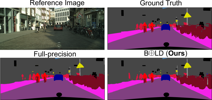
Figure 3: An example of cityscapes.

Table 7: bert models results. ^†Source code [66].

Method	GLUE Benchmark (Accuracy, $\uparrow$)
	mnli	qqp	qnli	sst-2	cola	sst-b	mrpc	rte	Avg.
fp bert	84.9	91.4	92.1	93.2	59.7	90.1	86.3	72.2	83.9
binarybert	35.6	66.2	51.5	53.2	0.0	6.1	68.3	52.7	41.0
bibert	66.1	84.8	72.6	88.7	25.4	33.6	72.5	57.4	63.2
bit	77.1	82.9	85.7	87.7	25.1	71.1	79.7	58.8	71.0
bit (Reprod.†)	76.8	87.2	85.6	87.5	24.1	70.5	78.9	58.8	69.7
( ) b$\oplus$ld	75.6	85.9	84.1	88.7	27.1	68.7	78.4	58.8	70.9

BERT fine-tuning for NLU tasks.

Finally, we consider fine-tuning bert [26], a transformer-based model [96], on the glue benchmark [98]. We follow the standard experimental protocol as in [26, 5, 78]. Our model and the chosen baselines are employed with 1-bit bitwidth for both weights and activations. Our Boolean bert model is inspired from bit [66] for binarizing activations, and incorporating kd during training, where the fp teacher guides the student in a layer-wise manner. As shown in Table 7, all methods suffer from performance drop compared to the fp model as extreme binarization of transformer-based model is not trivial. Nevertheless, our method yields results comparable to bit [66], the sota method on this task, outperforming binarybert [5] and bibert [78] on average. This is remarkable as our method natively uses Boolean weights during the training, whereas the baselines heavily rely on fp latent weights. These findings indicate potential for energy-efficient large language models (llms) using our method for both training and inference.

5 Conclusions

We have introduced a novel mathematical principle to define Boolean neural networks (nns) and Boolean Logic Backpropagation that extracts and synthesizes the essence of function minimization in logic rules, being the first to realize in-binary deep training natively, without approximation. Gradient becomes optional, not mandatory. We have extensively explored the capabilities of our method, highlighting: (i) both training and inference are now possible in binary; (ii) enlarged Boolean models recover fp performance while reducing complexity significantly; (iii) Boolean models can handle finer tasks beyond classification, contrary to common belief; (iv) deep training complexity can be drastically reduced to unprecedented levels. This innovation paves the way for greener deep learning and facilitates new applications like online, incremental, and on-device training. Broader impacts of our work is further discussed in Appendix F.

Limitations.

Due to current computing accelerators, such as GPUs, primarily designed for real arithmetic, our method could not be assessed on native Boolean accelerator. Nevertheless, its considerable potential may inspire the development of new logic circuits and architectures utilizing Boolean logic processing. While extensively tested on large models and datasets like imagenet, further application on extremely large models such as llms [13] holds promise for future endeavors.

Appendix

 

Appendix A Details of the Boolean Variation Method

A.1 Boolean Variation Calculus

With reference to Example 3.9, Table 8 gives the variation truth table of $f(x)=\mathbf{xor}(a,x)$, for $a,x\in\mathbb{B}$.

Table 8: Variation truth table of $f(x)=\mathbf{xor}(a,x)$, $a,x\in\mathbb{B}$.

$a$	$x$	$\neg x$	$\delta(x\to\neg x)$	$f(a,x)$	$f(a,\neg x)$	$\delta f(x\to\neg x)$	$f^{\prime}(x)$
$\mathrm{T}$	$\mathrm{T}$	$\mathrm{F}$	$\mathrm{F}$	$\mathrm{F}$	$\mathrm{T}$	$\mathrm{T}$	$\mathrm{F}$
$\mathrm{T}$	$\mathrm{F}$	$\mathrm{T}$	$\mathrm{T}$	$\mathrm{T}$	$\mathrm{F}$	$\mathrm{F}$	$\mathrm{F}$
$\mathrm{F}$	$\mathrm{T}$	$\mathrm{F}$	$\mathrm{F}$	$\mathrm{T}$	$\mathrm{F}$	$\mathrm{F}$	$\mathrm{T}$
$\mathrm{F}$	$\mathrm{F}$	$\mathrm{T}$	$\mathrm{T}$	$\mathrm{F}$	$\mathrm{T}$	$\mathrm{T}$	$\mathrm{T}$

We now proceed to the proof of Theorem 3.11.

Definition A.1 (Type conversion).

Define:

$$\operatorname{p}\colon \mathbb{N}\to\mathbb{L}$$

$$x\mapsto\operatorname{p}(x)=\begin{cases}\mathrm{T},&\textrm{if }x>0,\\ 0,&\textrm{if }x=0,\\ \mathrm{F},&\textrm{if }x<0.\end{cases}$$ (13)

$$\operatorname{e}\colon \mathbb{L}\to\mathbb{N}$$

$$a\mapsto\operatorname{e}(a)=\begin{cases}+1,&\textrm{if }a=\mathrm{T},\\ 0,&\textrm{if }a=0,\\ -1,&\textrm{if }a=\mathrm{F}.\end{cases}$$ (14)

$\operatorname{p}$ projects a numeric type in logic, and $\operatorname{e}$ embeds a logic type in numeric. The following properties are straightforward:

Proposition A.2.

The following properties hold:

1. $\forall x,y\in\mathbb{N}$: $\operatorname{p}(xy)=\mathbf{xnor}(\operatorname{p}(x),\operatorname{p}(y))$.

2. $\forall a,b\in\mathbb{L}$: $\operatorname{e}(\mathbf{xnor}(a,b))=\operatorname{e}(a)\operatorname{e}(b)$.

3. $\forall x,y\in\mathbb{N}$: $x=y\Leftrightarrow|x|=|y|\textrm{ and }\operatorname{p}(x)=\operatorname{p}(y)$.

In particular, property Proposition A.2(2) implies that by the embedding map $\operatorname{e}(\cdot)$, we have:

$$(\{\mathrm{T},\mathrm{F}\},\mathbf{xor}) \cong(\{\pm 1\},-\times),$$ (15)

$$(\{\mathrm{T},\mathrm{F}\},\mathbf{xnor}) \cong(\{\pm 1\},\times),$$ (16)

where $\cong$ and $\times$ stand for isomorphic relation, and the real multiplication, resp. A consequence is that by $\operatorname{e}(\cdot)$, a computing sequence of pointwise XOR/XNOR, counting, and majority vote is equivalent to a sequence of pointwise multiplications and accumulation performed on the embedded data. This property will be used in §§ A.2 and C for studying Boolean method using some results from bnns literature and real analysis.

Proposition A.3.

The following properties hold:

1. $a\in\mathbb{L}$, $x\in\mathbb{N}$: $\mathbf{xnor}(a,x)=\operatorname{e}(a)x$.

2. $x,y\in\mathbb{N}$: $\mathbf{xnor}(x,y)=xy$.

3. $x\in\{\mathbb{L},\mathbb{N}\}$, $y,z\in\mathbb{N}$: $\mathbf{xnor}(x,y+z)=\mathbf{xnor}(x,y)+\mathbf{xnor}(x,z)$.

4. $x\in\{\mathbb{L},\mathbb{N}\}$, $y,\lambda\in\mathbb{N}$: $\mathbf{xnor}(x,\lambda y)=\lambda\mathbf{xnor}(x,y)$.

5. $x\in\{\mathbb{L},\mathbb{N}\}$, $y\in\mathbb{N}$: $\mathbf{xor}(x,y)=-\mathbf{xnor}(x,y)$.

Proof.

The proof follows definitions 3.5 and A.1.

• Following Definition 3.1 we have $\forall t\in\mathbb{M}$, $\mathbf{xnor}(\mathrm{T},t)=t$, $\mathbf{xnor}(\mathrm{F},t)=\neg t$, and $\mathbf{xnor}(0,t)=0$. Put $v=\mathbf{xnor}(a,x)$. We have $|v|=|x|$ and $\operatorname{p}(v)=\mathbf{xnor}(a,\operatorname{p}(x))$. Hence, $a=0\Rightarrow\operatorname{p}(v)=0\Rightarrow v=0$; $a=\mathrm{T}\Rightarrow\operatorname{p}(v)=\operatorname{p}(x)\Rightarrow v=x$; $a=\mathrm{F}\Rightarrow\operatorname{p}(v)=\neg\operatorname{p}(x)\Rightarrow v=-x$. Hence (1).

• The result is trivial if $x=0$ or $y=0$. For $x,y\neq 0$, put $v=\mathbf{xnor}(x,y)$, we have $|v|=|x||y|$ and $\operatorname{p}(v)=\mathbf{xnor}(\operatorname{p}(x),\operatorname{p}(y))$. According to Definition A.1, if $\operatorname{sign}(x)=\operatorname{sign}(y)$, we have $\operatorname{p}(v)=\mathrm{T}\Rightarrow v=|x||y|=xy$. Otherwise, i.e., $\operatorname{sign}(x)=-\operatorname{sign}(y)$, $\operatorname{p}(v)=\mathrm{F}\Rightarrow v=-|x||y|=xy$. Hence (2).

• (3) and (4) follow (1) for $x\in\mathbb{L}$ and follow (2) for $x\in\mathbb{N}$.

• For (5), write $u=\mathbf{xor}(x,y)$ and $v=\mathbf{xnor}(x,y)$, we have $|u|=|v|$ and $\operatorname{p}(u)=\mathbf{xor}(\operatorname{p}(x),\operatorname{p}(y))=\neg\mathbf{xnor}(\operatorname{p}(x),\operatorname{p}(y))=\neg\operatorname{p}(v)$. Thus, $\operatorname{sign}(u)=-\operatorname{sign}(v)\Rightarrow u=-v$. ∎

Proposition A.4.

For $f,g\in\mathcal{F}(\mathbb{B},\mathbb{B})$, $\forall x,y\in\mathbb{B}$ the following properties hold:

1. $\delta f(x\to y)=\mathbf{xnor}(\delta(x\to y),f^{\prime}(x)).$

2. $(\neg f)^{\prime}(x)=\neg f^{\prime}(x)$.

3. $(g\circ f)^{\prime}(x)=\mathbf{xnor}(g^{\prime}(f(x)),f^{\prime}(x))$.

Proof.

The proof is by definition:

1. $\forall x,y\in\mathbb{B}$, there are two cases. If $y=x$, then the result is trivial. Otherwise, i.e., $y=\neg x$, by definition we have:

   $$f^{\prime}(x) =\mathbf{xnor}(\delta(x\to\neg x),\delta f(x\to\neg x))$$

   $$\Leftrightarrow\quad\delta f(x\to\neg x) =\mathbf{xnor}(\delta(x\to\neg x),f^{\prime}(x)).$$

   Hence the result.

2. $\forall x,y\in\mathbb{B}$, it is easy to verify by truth table that $\delta(\neg f(x\to y))=\neg\delta f(x\to y)$. Hence, by definition,

   $$(\neg f)^{\prime}(x) =\mathbf{xnor}(\delta(x\to\neg x),\delta(\neg f(x\to\neg x)))$$

   $$=\mathbf{xnor}(\delta(x\to\neg x),\neg\delta f(x\to\neg x))$$

   $$=\neg\mathbf{xnor}(\delta(x\to\neg x),\delta f(x\to\neg x))$$

   $$=\neg f^{\prime}(x).$$

3. Using definition, property (i), and associativity of $\mathbf{xnor}$, $\forall x\in\mathbb{B}$ we have:

   $$(g\circ f)^{\prime}(x) =\mathbf{xnor}(\delta(x\to\neg x),\delta g(f(x)\to f(\neg x)))$$

   $$=\mathbf{xnor}\left(\delta(x\to\neg x),\mathbf{xnor}\left(\delta f(x\to\neg x),g^{\prime}\left(f(x)\right)\right)\right)$$

   $$=\mathbf{xnor}\left(g^{\prime}(f(x)),\mathbf{xnor}\left(\delta(x\to\neg x),\delta f(x\to\neg x)\right)\right)$$

   $$=\mathbf{xnor}(g^{\prime}(f(x)),f^{\prime}(x)).$$

   ∎

Proposition A.5.

For $f\in\mathcal{F}(\mathbb{B},\mathbb{N})$, the following properties hold:

1. $x,y\in\mathbb{B}$: $\delta f(x\to y)=\mathbf{xnor}(\delta(x\to y),f^{\prime}(x))$.

2. $x\in\mathbb{B}$, $\alpha\in\mathbb{N}$: $(\alpha f)^{\prime}(x)=\alpha f^{\prime}(x)$.

3. $x\in\mathbb{B}$, $g\in\mathcal{F}(\mathbb{B},\mathbb{N})$: $(f+g)^{\prime}(x)=f^{\prime}(x)+g^{\prime}(x)$.

Proof.

The proof is as follows:

1. For $x,y\in\mathbb{B}$. Firstly, the result is trivial if $y=x$. For $y\neq x$, i.e., $y=\neg x$, by definition:

   $$f^{\prime}(x)=\mathbf{xnor}(\delta(x\to\neg x),\delta f(x\to\neg x)).$$

   Hence, $|\delta f(x\to\neg x)|=|f^{\prime}(x)|$ since $|\delta(x\to\neg x)|=1$, and

   $$\operatorname{p}(f^{\prime}(x)) =\mathbf{xnor}(\delta(x\to\neg x),\operatorname{p}(\delta f(x\to\neg x)))$$

   $$\Leftrightarrow\quad\operatorname{p}(\delta f(x\to\neg x)) =\mathbf{xnor}(\delta(x\to\neg x),\operatorname{p}(f^{\prime}(x))),$$

   where $\operatorname{p}(\cdot)$ is the logic projector Eq. 13. Thus, $\delta f(x\to\neg x)=\mathbf{xnor}(\delta(x\to\neg x),f^{\prime}(x))$. Hence the result.

2. Firstly $\forall x,y\in\mathbb{B}$, we have

   $$\delta(\alpha f(x\to y))=\alpha f(y)-\alpha f(x)=\alpha\delta f(x\to y).$$

   Hence, by definition,

   $$(\alpha f)^{\prime}(x) =\mathbf{xnor}(\delta(x\to\neg x),\delta(\alpha f(x\to\neg x)))$$

   $$=\mathbf{xnor}(\delta(x\to\neg x),\alpha\delta f(x\to\neg x))$$

   $$=\alpha\,\mathbf{xnor}(\delta(x\to\neg x),\delta f(x\to\neg x)),\textrm{ due to \lx@cref{creftype~refnum}{prop:XNORAlgebra}(4)}$$

   $$=\alpha f^{\prime}(x).$$

3. For $f,g\in\mathcal{F}(\mathbb{B},\mathbb{N})$,

   $$(f+g)^{\prime}(x) =\mathbf{xnor}(\delta(x\to\neg x),\delta(f+g)(x\to\neg x))$$

   $$=\mathbf{xnor}(\delta(x\to\neg x),\delta f(x\to\neg x)+\delta g(x\to\neg x))$$

   $$\overset{(*)}{=}\mathbf{xnor}(\delta(x\to\neg x),\delta f(x\to\neg x))+\mathbf{xnor}(\delta(x\to\neg x),\delta g(x\to\neg x)),$$

   $$=f^{\prime}(x)+g^{\prime}(x),$$

   where $(*)$ is due to Proposition A.3(3). ∎

Proposition A.6 (Composition rules).

The following properties hold:

1. For $\mathbb{B}\overset{f}{\to}\mathbb{B}\overset{g}{\to}\mathbb{D}$: $(g\circ f)^{\prime}(x)=\mathbf{xnor}(g^{\prime}(f(x)),f^{\prime}(x))$, $\forall x\in\mathbb{B}$.

2. For $\mathbb{B}\overset{f}{\to}\mathbb{Z}\overset{g}{\to}\mathbb{D}$, $x\in\mathbb{B}$, if $|f^{\prime}(x)|\leq 1$ and $g^{\prime}(f(x))=g^{\prime}(f(x)-1)$, then:

   $$(g\circ f)^{\prime}(x)=\mathbf{xnor}(g^{\prime}(f(x)),f^{\prime}(x)).$$

Proof.

The proof is as follows.

1. The case of $\mathbb{B}\overset{f}{\to}\mathbb{B}\overset{g}{\to}\mathbb{B}$ is obtained from Proposition A.4(3). For $\mathbb{B}\overset{f}{\to}\mathbb{B}\overset{g}{\to}\mathbb{N}$, by using Proposition A.5(1), the proof is similar to that of Proposition A.4(3).

2. By definition, we have

   $$(g\circ f)^{\prime}(x)=\mathbf{xnor}(\delta(x\to\neg x),\delta g(f(x)\to f(\neg x))).$$ (17)

   Using property (1) of Proposition A.5, we have:

   $$f(\neg x) =f(x)+\delta f(x\to\neg x)$$

   $$=f(x)+\mathbf{xnor}(\delta(x\to\neg x),f^{\prime}(x)).$$ (18)

   Applying Eq. 18 back to Eq. 17, the result is trivial if $f^{\prime}(x)=0$. The remaining case is $|f^{\prime}(x)|=1$ for which we have $\mathbf{xnor}(\delta(x\to\neg x),f^{\prime}(x))=\pm 1$. First, for $\mathbf{xnor}(\delta(x\to\neg x),f^{\prime}(x))=1$, we have:

   $$\delta g(f(x)\to f(\neg x)) =\delta g(f(x)\to f(x)+1)$$

   $$=g^{\prime}(f(x))$$

   $$=\mathbf{xnor}(g^{\prime}(f(x)),1)$$

   $$=\mathbf{xnor}(g^{\prime}(f(x)),\mathbf{xnor}(\delta(x\to\neg x),f^{\prime}(x))).$$ (19)

   Substitute Eq. 19 back to Eq. 17, we obtain:

   $$(g\circ f)^{\prime}(x) =\mathbf{xnor}(\delta(x\to\neg x),\delta g(f(x)\to f(\neg x)))$$

   $$=\mathbf{xnor}(\delta(x\to\neg x),\mathbf{xnor}(g^{\prime}(f(x)),\mathbf{xnor}(\delta(x\to\neg x),f^{\prime}(x))))$$

   $$=\mathbf{xnor}(g^{\prime}(f(x)),f^{\prime}(x)),$$

   where that last equality is by the associativity of $\mathbf{xnor}$ and that $\mathbf{xnor}(x,x)=\mathrm{T}$ for $x\in\mathbb{B}$. Similarly, for $\mathbf{xnor}(\delta(x\to\neg x),f^{\prime}(x))=-1$, we have:

   $$\delta g(f(x)\to f(\neg x)) =\delta g(f(x)\to f(x)-1)$$

   $$=-g^{\prime}(f(x)-1)$$

   $$=\mathbf{xnor}(g^{\prime}(f(x)-1),-1)$$

   $$=\mathbf{xnor}(g^{\prime}(f(x)-1),\mathbf{xnor}(\delta(x\to\neg x),f^{\prime}(x))).$$ (20)

   Substitute Eq. 20 back to Eq. 17 and use the assumption that $g^{\prime}(f(x))=g^{\prime}(f(x)-1)$, we have:

   $$(g\circ f)^{\prime}(x) =\mathbf{xnor}(\delta(x\to\neg x),\delta g(f(x)\to f(\neg x)))$$

   $$=\mathbf{xnor}(\delta(x\to\neg x),\mathbf{xnor}(g^{\prime}(f(x)-1),\mathbf{xnor}(\delta(x\to\neg x),f^{\prime}(x))))$$

   $$=\mathbf{xnor}(g^{\prime}(f(x)),f^{\prime}(x)).$$

   Hence the result. ∎

The results of Theorem 3.11 are from Propositions A.4, A.5 and A.6.

A.2 Convergence Proof

To the best of our knowledge, in the quantized neural network literature and in particular bnn, one can only prove the convergence up to an irreducible error floor [60]. This idea has been extended to SVRG [25], and recently to SGLD in [111], which is also up to an error limit.

In this section we provide complexity bounds for Boolean Logic in a smooth non-convex environment. We introduce an abstraction to model its optimization process and prove its convergence.

A.2.1 Continuous Abstraction

Boolean optimizer is discrete, proving its convergence directly is a hard problem. The idea is to find a continuous equivalence so that some proof techniques existing from the bnn and quantized neural networks literature can be employed. We also abstract the logic optimization rules as compressor $Q_{0}(),Q_{1}()$, and define gradient accumulator $a_{t}$ as $a_{t+1}=a_{t}+\varphi(q_{t})$. When $\eta$ is constant, we recover the definition (10) and obtain $m_{t}=\eta a_{t}$. Our analysis is based on the following standard non-convex assumptions on $f$:

A. 1.

Uniform Lower Bound: There exists $f_{*}\in\mathbb{R}$ s.t. $f(w)\geq f_{*}$, $\forall w\in\mathbb{R}^{d}$.

A. 2.

Smooth Derivatives: The gradient $\nabla f(w)$ is $L$-Lipschitz continuous for some $L>0$, i.e., $\forall w,\forall v\in\mathbb{R}^{d}$: $\left\|\nabla f(w)-\nabla f(v)\right\|\leq L\|w-v\|.$

A. 3.

Bounded Variance: The variance of the stochastic gradients is bounded by some $\sigma^{2}>0$, i.e., $\forall w\in\mathbb{R}^{d}$: $\mathbb{E}\left[\tilde{\nabla}f(w)\right]=\nabla f(w)$ and $\mathbb{E}\left[\|\tilde{\nabla}f(w)\|^{2}\right]\leq\sigma^{2}.$

A. 4.

Compressor: There exists $\gamma<1$ s.t. $\forall w,\forall v\in\mathbb{R}^{d}$, $\|Q_{1}(v,w)-v\|^{2}\leq\gamma\|v\|^{2}$.

A. 5.

Bounded Accumulator: There exists $\kappa\in\mathbb{R}^{*}_{+}$ s.t. $\forall t$ and $\forall i\in[d]$, we have $|a_{t}|_{i}\leq\kappa$.

A. 6.

Stochastic Flipping Rule: For all $w\in\mathbb{R}^{d}$, we have $\mathbb{E}\left[Q_{0}(w)|w\right]=w$.

In existing frameworks, quantity $\tilde{\nabla}f(\cdot)$ denotes the stochastic gradient computed on a random mini-batch of data. Boolean framework does not have the notion of gradient, it however has an optimization signal (i.e., $\varphi$(q) or its accumulator $m_{t}$ (10)) that plays the same role as $\tilde{\nabla}f(\cdot)$. Therefore, these two notions, i.e., continuous gradient and Boolean optimization signal, can be encompassed into a generalized notion. That is the root to the following continuous relaxation in which $\tilde{\nabla}f(\cdot)$ standards for the optimization signal computed on a random mini-batch of data.

For reference, the original Boolean optimizer as formulated in § 3 is summarized in Algorithm 2 in which $\texttt{flip}(w_{t},m_{t+1})$ flips weight and $\texttt{reset}(w_{t},m_{t+1})$ resets its accumulator when the flip condition is triggered.

1 $m_{t+1}\leftarrow\beta_{t}m_{t}+\eta\varphi(q_{t})$ ;

2 $w_{t+1}\leftarrow\texttt{flip}(w_{t},m_{t+1})$;

3 $m_{t+1}\leftarrow\texttt{reset}(w_{t},m_{t+1})$;

Algorithm 2 Boolean optimizer

Data: $Q_{0},Q_{1}$ quantizer

1 $m_{t}\leftarrow\eta\tilde{\nabla}f(w_{t})+e_{t}$;

2 $\Delta_{t}\leftarrow Q_{1}(m_{t},w_{t})$;

3 $w_{t+1}\leftarrow Q_{0}(w_{t}-\Delta_{t})$;

4 $e_{t+1}\leftarrow m_{t}-\Delta_{t}$;

Algorithm 3 Equivalent formulation of Boolean optimizer

Algorithm 3 describes an equivalent formulation of Boolean optimizer. Therein, $Q_{0}$, $Q_{1}$ are quantizers which are specified in the following. Note that EF-SIGNSGD (SIGNSGD with Error-Feedback) algorithm from [52] is a particular case of this formulation with $Q_{0}()=\operatorname{Identity}()$ and $Q_{1}()=\operatorname{sign}()$. For Boolean Logic abstraction, they are given by:

$$\begin{cases}Q_{1}(m_{t},w_{t})=w_{t}(\textrm{ReLu}(w_{t}m_{t}-1)+\frac{1}{2}\operatorname{sign}(w_{t}m_{t}-1)+\frac{1}{2}),\\ Q_{0}(w_{t})=\operatorname{sign}(w_{t}).\end{cases}$$ (21)

The combination of $Q_{1}$ and $Q_{0}$ is crucial to take into account the reset property of the accumulator $m_{t}$. Indeed in practice, $\Delta_{t}:=Q_{1}({m_{t}},w_{t})$ is always equal to $0$ except when $|m_{t}|>1$ and $\operatorname{sign}(m_{t})=\operatorname{sign}(w_{t})$ (i.e., when the flipping rule is applied). As $w_{t}$ has only values in $\{\pm 1\}$, $Q_{0}$ acts as identity function, except when $\Delta_{t}$ is non-zero (i.e., when the flipping rule is applied). With the choices (21), we can identify $\texttt{flip}(w_{t},m_{t})=Q_{0}(w_{t}-Q_{1}(m_{t},w_{t}))$. We do not have closed-form formula for $\texttt{reset}(w_{t},m_{t+1})$ from Algorithm 2, but the residual errors $e_{t}$ play this role. Indeed, $e_{t+1}=m_{t}$ except when $\Delta_{t}$ is non-zero (i.e., when the flipping rule is applied and $e_{t+1}$ is equal to $0$).

The main difficulty in the analysis comes from the parameters quantization $Q_{0}()$. Indeed, we can follow the derivations in Appendix B.3 from [52] to bound the error term $\mathbb{E}\left[\|e_{t}\|^{2}\right]$, but we also have additional terms coming from the quantity:

$$h_{t}=Q_{0}(w_{t}-Q_{1}(m_{t},w_{t}))-(w_{t}-Q_{1}(m_{t},w_{t})).$$ (22)

As a consequence, assumptions 1 to 6 enable us to obtain $\mathbb{E}\left[h_{t}\right]=0$ and to bound the variance of $h_{t}$.

Remark A.7.

Assumptions 1 to 3 are standard. Assumptions 4 to 6 are non-classic but dedicated to Boolean Logic strategy. 4 is equivalent to assuming Boolean Logic optimization presents at least one flip at every iteration $t$. 4 is classic in the literature of compressed SGD [52, 4, 77]. Moreover, 5 and 6 are not restrictive, but algorithmic choices. For example, rounding ($Q_{0}$ function) can be stochastic based on the value of the accumulator $m_{t}$. Similar to STE clipping strategy, the accumulator can be clipped to some pre-defined value $\kappa$ before applying the flipping rule to verify 5.

Remark A.8.

Our proof assumes that the step size $\eta$ is constant over iterations. But in practice, we gently decrease the value of $\eta$ at some time steps. Our proof can be adapted to this setting by defining a gradient accumulator $a_{t}$ such that $a_{t+1}=a_{t}+\varphi(q_{t})$. When $\eta$ is constant we recover the definition (10) and we obtain $m_{t}=\eta a_{t}$. In the proposed algorithm, gradients are computed on binary weight $w_{t}$ and accumulated in $a_{t}$. Then, one applies the flipping rule on the quantity $\tilde{w}_{t}=\eta a_{t}$ ($\tilde{w}_{t}=m_{t}$ when $\eta$ is constant), and one (may) reset the accumulator $a_{t}$.

We start by stating a key lemma which shows that the residual errors $e_{t}$ maintained in Algorithm 3 do not accumulate too much.

Lemma A.9.

Under 3 and 4, the error can be bounded as $\mathbb{E}\left[\|e_{t}\|^{2}\right]\leq\frac{2\gamma}{(1-\gamma)^{2}}\eta^{2}\sigma^{2}$.

Proof.

We start by using the definition of the error sequence:

$$\|e_{t+1}\|^{2}=\|Q_{1}(m_{t},w_{t})-m_{t}\|^{2}.$$

Next we make use of 4:

$$\|e_{t+1}\|^{2}\leq\gamma\|m_{t}\|^{2}.$$

We develop the accumulator update:

$$\|e_{t+1}\|^{2}\leq\gamma\|e_{t}+\eta\tilde{\nabla}f(w_{t})\|^{2}.$$

We thus have a recurrence relation on the bound of $e_{t}$. Using Young’s inequality, we have that for any $\beta>0$,

$$\|e_{t+1}\|^{2}\leq\gamma(1+\beta)\|e_{t}\|^{2}+\gamma(1+\frac{1}{\beta})\eta^{2}\|\tilde{\nabla}f(w_{t})\|^{2}.$$

Rolling the recursion over and using 3 we obtain:

$$\mathbb{E}\left[\|e_{t+1}\|^{2}\right]\leq \gamma(1+\beta)\mathbb{E}\left[\|e_{t}\|^{2}\right]+\gamma(1+\frac{1}{\beta})\eta^{2}\mathbb{E}\left[\|\tilde{\nabla}f(w_{t})\|^{2}\right]$$

$$\leq \gamma(1+\beta)\mathbb{E}\left[\|e_{t}\|^{2}\right]+\gamma(1+\frac{1}{\beta})\eta^{2}\sigma^{2}$$

$$\leq \sum_{r}^{t}(\gamma(1+\beta))^{r}\gamma(1+\frac{1}{\beta})\eta^{2}\sigma^{2}$$

$$\leq \frac{\gamma(1+\frac{1}{\beta})}{1-\gamma(1+\beta)}\eta^{2}\sigma^{2}.$$

Take $\beta=\frac{1-\gamma}{2\gamma}$ and plug it in the above bounds gives:

$$\mathbb{E}\left[\|e_{t+1}\|^{2}\right]\leq\frac{2\gamma}{(1-\gamma)^{2}}\eta^{2}\sigma^{2}.$$

∎

Then, the next Lemma allows us to bound the averaged norm-squared of the distance between the Boolean weight and $w_{t}-Q_{1}(m_{t},w_{t})$. We make use of the previously defined quantity $h_{t}$ (22) and have:

Lemma A.10.

Under assumptions 5 and 6: $\mathbb{E}\left[\|h_{t}\|^{2}\right]\leq\eta d\kappa$.

Proof.

Let consider a coordinate $i\in[d]$. $Q_{0}|_{i}$ as $-1$ or $+1$ for value with some probability $p_{i,t}$. For the ease of presentation, we will drop the subscript $i$. Denote $u_{t}:=w_{t}-Q_{1}(m_{t},w_{t})$. Hence, $h_{t}$ can take value $(1-u_{t})$ with some probability $p_{t}$ and $(-1-u_{t})$ with probability $1-p_{t}$. Assumption 6 yields $2p_{t}-1=u_{t}$. Therefore, we can compute the variance of $h_{t}$ as follows:

$$\mathbb{E}\left[\|h_{t}\|^{2}\right] =\mathbb{E}\left[\sum_{i}^{d}1+(w_{t}-Q_{1}(m_{t},w_{t}))^{2}-2Q_{0}(w_{t}-Q_{1}(m_{t},w_{t})(w_{t}-Q_{1}(m_{t},w_{t})\right]$$

$$=\sum_{i}^{d}((1-u_{t})^{2}p_{t}+(-1-u_{t})^{2}(1-p_{t}))$$

$$=\sum_{i}^{d}(1-u_{t}^{2}).$$

The definition of $u_{t}$ leads to

$$1-u_{t}^{2} =1-(1+Q_{1}(m_{t},w_{t})^{2}-2w_{t}Q_{1}(m_{t},w_{t}))$$

$$=Q_{1}(m_{t},w_{t})(2w_{t}-Q_{1}(m_{t},w_{t})).$$

When $m_{t}<1$, we directly have $Q_{1}(m_{t},w_{t})(2w_{t}-Q_{1}(m_{t},w_{t}))=0\leq\eta\kappa$. When $m_{t}\geq 1$, we apply the definition of $Q_{1}$ to obtain:

$$Q_{1}(m_{t},w_{t})(2w_{t}-Q_{1}(m_{t},w_{t})) \leq m_{t}(2-m_{t})$$

$$\leq\eta\kappa.$$

Therefore, we can apply this result to every coordinate, and conclude that:

$$\mathbb{E}\left[\|h_{t}\|^{2}\right]\leq\eta d\kappa.$$ (23)

∎

A.2.2 Proof of Theorem 3.16

We now can proceed to the proof of Theorem 3.16.

Proof.

Consider the virtual sequence $x_{t}=w_{t}-e_{t}$. We have:

$$x_{t+1} =Q_{0}(w_{t}-\Delta_{t})-(m_{t}-\Delta_{t})$$

$$=(Q_{0}(w_{t}-\Delta_{t})+\Delta_{t}-e_{t})-\eta\tilde{\nabla}f(w_{t}).$$

Considering the expectation with respect to the random variable $Q_{0}$ and the gradient noise, we have:

$$\mathbb{E}\left[x_{t+1}|w_{t}\right]=x_{t}-\eta\nabla f(w_{t}).$$

We consider $\mathbb{E}_{t}\left[\cdot\right]$ the expectation with respect to every random process know up to time $t$. We apply the $L$-smoothness assumption 2, and assumptions 3, 6 to obtain:

$$\mathbb{E}_{t}\left[f(x_{t+1})-f(x_{t})\right] \leq-\eta\langle\nabla f(x_{t}),\nabla f(w_{t})\rangle+\frac{L}{2}\mathbb{E}_{t}\left[\|(Q_{0}(w_{t}-\Delta_{t})+\Delta_{t})-\eta\tilde{\nabla}f(w_{t})-w_{t}\|^{2}\right].$$

We now reuse $h_{t}$ from (22) and simplify the above:

$$\mathbb{E}_{t}\left[f(x_{t+1})-f(x_{t})\right] \leq-\eta\langle\nabla f(x_{t}),\nabla f(w_{t})\rangle+\frac{L}{2}\mathbb{E}_{t}\left[\|h_{t}-\eta\tilde{\nabla}f(w_{t})\|^{2}\right]$$

$$\leq-\eta\langle\nabla f(x_{t})-\nabla f(w_{t})+\nabla f(w_{t}),\nabla f(w_{t})\rangle+\frac{L}{2}\mathbb{E}_{t}\left[\|h_{t}-\eta\tilde{\nabla}f(w_{t})\|^{2}\right].$$

Using Young’s inequality, we have that for any $\beta>0$,

$$\mathbb{E}_{t}\left[f(x_{t+1})-f(x_{t})\right]\leq -\eta\langle\nabla f(x_{t})-\nabla f(w_{t})+\nabla f(w_{t}),\nabla f(w_{t})\rangle$$

$$+\frac{L}{2}(1+\beta)\mathbb{E}_{t}\left[\|h_{t}\|^{2}\right]+\frac{L}{2}\eta^{2}(1+\frac{1}{\beta})\sigma^{2}.$$

Making use again of smoothness and Young’s inequality we have:

$$\mathbb{E}_{t}\left[f(x_{t+1})-f(x_{t})\right]\leq -\eta\|\nabla f(w_{t})\|^{2}-\eta\langle\nabla f(x_{t})-\nabla f(w_{t}),\nabla f(w_{t})\rangle$$

$$+\frac{L}{2}(1+\beta)\mathbb{E}_{t}\left[\|h_{t}\|^{2}\right]+\frac{L}{2}\eta^{2}(1+\frac{1}{\beta})\sigma^{2}$$

$$\leq -\eta\|\nabla f(w_{t})\|^{2}+\frac{\eta\rho}{2}\|\nabla f(w_{t})\|^{2}+\frac{\eta}{2\rho}\|\nabla f(x_{t})-\nabla f(w_{t})\|^{2}$$

$$+\frac{L}{2}(1+\beta)\mathbb{E}_{t}\left[\|h_{t}\|^{2}\right]+\frac{L}{2}\eta^{2}(1+\frac{1}{\beta})\sigma^{2}$$

$$\leq -\eta\|\nabla f(w_{t})\|^{2}+\frac{\eta\rho}{2}\|\nabla f(w_{t})\|^{2}+\frac{\eta L^{2}}{2\rho}\underbrace{\|x_{t}-w_{t}\|^{2}}_{\|e_{t}\|^{2}}$$

$$+\frac{L}{2}(1+\beta)\mathbb{E}_{t}\left[\|h_{t}\|^{2}\right]+\frac{L}{2}\eta^{2}(1+\frac{1}{\beta})\sigma^{2}.$$

Under the law of total expectation, we make use of Lemma A.9 and Lemma A.10 to obtain:

$$\mathbb{E}\left[f(x_{t+1})\right]-\mathbb{E}\left[f(x_{t})\right]\leq -\eta(1-\frac{\rho}{2})\mathbb{E}\left[\|\nabla f(w_{t})\|^{2}\right]+\frac{\eta L^{2}}{2\rho}\frac{4\gamma}{(1-\gamma)^{2}}\eta^{2}\sigma^{2}$$

$$+\frac{L}{8}\eta(1+\beta)d\kappa+\frac{L}{2}\eta^{2}(1+\frac{1}{\beta})\sigma^{2}.$$

Rearranging the terms and averaging over $t$ gives for $\rho<2$ (we can choose for instance $\rho=\beta=1$):

$$\frac{1}{T+1}\sum_{t=0}^{T}\|\nabla f(w_{t})\|^{2}\leq\frac{2(f(w_{0})-f_{*})}{\eta(T+1)}+2L\sigma^{2}\eta+4L^{2}\sigma^{2}\frac{\gamma}{(1-\gamma)^{2}}\eta^{2}+\frac{L}{2}d\kappa.$$

∎

The bound in Theorem 3.16 contains 4 terms. The first term is standard for a general non-convex target and expresses how initialization affects convergence. The second and third terms depend on the fluctuation of the minibatch gradients. Another important aspect of the rate determined by Theorem 3.16 is its dependence on the quantization error. Note that there is an “error bound” of $\frac{L}{2}d\kappa$ that remains independent of the number of update iterations. The error bound is the cost of using discrete weights as part of the optimization algorithm. Previous work with quantized models also includes error bounds [60, 61].

Appendix B Code Sample of Core Implementation

In this section we provide example codes in Python of a Boolean linear layer that employs $\mathbf{xor}$ logic kernel. This implementation is in particular based on PyTorch [76]. The class of Boolean linear layer is defined in Algorithm 4; and its backpropagation mechanism, overwritten from autograd, is shown in Algorithm 5. Here, we consider both cases of the received backpropagation signal $Z$ as described in Fig. 2, which are either Boolean (see Algorithm 6) or real-valued (see Algorithm 7). An example code of the Boolean optimizer is provided in Algorithm 8.

Notice that our custom XORLinear layer can be flexibly combined with any fp PyTorch modules to define a model. The parameters of this layer are optimized by the BooleanOptimizer, whereas those of fp layers are optimized by a common fp optimizer like Adam [53].

1

⬇

1import torch

2

3from torch import Tensor, nn, autograd

4from typing import Any, List, Optional, Callable

5

6

7class XORLinear(nn.Linear):

8

9 def __init__(self, in_features: int, out_features: int, bool_bprop: bool, **kwargs):

10 super(XORLinear, self).__init__(in_features, out_features, **kwargs)

11 self.bool_bprop = bool_bprop

12

13 def reset_parameters(self):

14 self.weight = nn.Parameter(torch.randint(0, 2, self.weight.shape))

15

16 if self.bias is not None:

17 self.bias = nn.Parameter(torch.randint(0, 2, (self.out_features,)))

18

19 def forward(self, X):

20 return XORFunction.apply(X, self.weight, self.bias, self.bool_bprop)

Algorithm 4 Python code of xor linear layer

1

⬇

1class XORFunction(autograd.Function):

2

3 @staticmethod

4 def forward(ctx, X, W, B, bool_bprop: bool):

5 ctx.save_for_backward(X,W,B)

6 ctx.bool_bprop = bool_bprop

7

8 # Elementwise XOR logic

9 S = torch.logical_xor(X[:,None,:], W[None,:,:])

10

11 # Sum over the input dimension

12 S = S.sum(dim=2) + B

13

14 # 0-centered for use with BatchNorm when preferred

15 S = S - W.shape[1]/2

16

17 return S

18

19 @staticmethod

20 def backward(ctx, Z):

21 if ctx.bool_bprop:

22 G_X, G_W, G_B = backward_bool(ctx, Z)

23 else:

24 G_X, G_W, G_B = backward_real(ctx, Z)

25

26 return G_X, G_W, G_B, None

Algorithm 5 Python code of the backpropagation logic of xor linear layer

1

⬇

1def backward_bool(ctx, Z):

2 """

3 Variation of input:

4 - delta(xor(x,w))/delta(x) = neg w

5 - delta(Loss)/delta(x) = xnor(z,neg w) = xor(z,w)

6 Variation of weights:

7 - delta(xor(x,w))/delta(w) = neg x

8 - delta(Loss)/delta(x) = xnor(z,neg x) = xor(z,x)

9 Variation of bias:

10 - bias = xnor(bias,True) ==> Variation of bias is driven in

11 the same basis as that of weight with xnor logic and input True.

12 Aggregation:

13 - Count the number of TRUEs = sum over the Boolean data

14 - Aggr = TRUEs - FALSEs = TRUEs - (TOT - TRUEs) = 2TRUES - TOT

15 where TOT is the size of the aggregated dimension

16 """

17 X, W, B = ctx.saved_tensors

18

19 # Boolean variation of input

20 G_X = torch.logical_xor(Z[:,:,None], W[None,:,:])

21

22 # Aggregate over the out_features dimension

23 G_X = 2 * G_X.sum(dim=1) - W.shape[0]

24

25 # Boolean variation of weights

26 G_W = torch.logical_xor(Z[:,:,None], X[:,None,:])

27

28 # Aggregate over the batch dimension

29 G_W = 2 * G_W.sum(dim=0) - X.shape[0]

30

31 # Boolean variation of bias

32 if B is not None:

33 # Aggregate over the batch dimension

34 G_B = 2 * Z.sum(dim=0) - Z.shape[0]

35

36 # Return

37 return G_X, G_W, G_B

Algorithm 6 Backpropagation logic with Boolean received backpropagation

1

⬇

1def backward_real(ctx, Z):

2 X, W, B = ctx.saved_tensors

3

4 """

5 Boolean variation of input processed using torch avoiding loop:

6 -> xor(Z: Real, W: Boolean) = -Z * emb(W)

7 -> emb(W): T->1, F->-1 => emb(W) = 2W-1

8 => delta(Loss)/delta(X) = Z*(1-2W) """

9 G_X = Z.mm(1-2*W)

10

11 """

12 Boolean variation of weights processed using torch avoiding loop:

13 -> xor(Z: Real, X: Boolean) = -Z * emb(X)

14 -> emb(X): T->1, F->-1 => emb(X) = 2X-1

15 => delta(Loss)/delta(W) = Z^T * (1-2X) """

16 G_W = Z.t().mm(1-2*X)

17

18 """ Boolean variation of bias """

19 if B is not None:

20 G_B = Z.sum(dim=0)

21

22 # Return

23 return G_X, G_W, G_B

Algorithm 7 Backpropagation logic with real received backpropagation

1

⬇

1class BooleanOptimizer(torch.optim.Optimizer):

2

3 def __init__(self, params, lr: float):

4 super(BooleanOptimizer, self).__init__(params, dict(lr=lr))

5 for param_group in self.param_groups:

6 param_group[’accums’] = [torch.zeros_like(p.data) for p in param_group[’params’]]

7 param_group[’ratios’] = [0 for p in param_group[’params’]]

8 self._nb_flips = 0

9

10 @property

11 def nb_flips(self):

12 n = self._nb_flips

13 self._nb_flips = 0

14 return n

15

16 def step(self):

17 for param_group in self.param_groups:

18 for idx, p in enumerate(param_group[’params’]):

19 self.update(p, param_group, idx)

20

21 def update(self, param: Tensor, param_group: dict, idx: int):

22 accum = param_group[’ratios’][idx] * param_group[’accums’][idx] + param_group[’lr’] * param.grad.data

23 param_group[’accums’][idx] = accum

24 param_to_flip = accum * (2*param.data-1) >= 1

25 param.data[param_to_flip] = torch.logical_not(param.data[param_to_flip])

26 param_group[’accums’][idx][param_to_flip] = 0.

27 param_group[’ratios’][idx] = 1 - param_to_flip.float().mean()

28 self._nb_flips += float(param_to_flip.float().sum())

Algorithm 8 Python code of Boolean optimizer

Appendix C Training Regularization

C.1 Summary of the Main Techniques

Due to the binary activation, the effect on the loss function by an action on weight $w$ diminishes with the distance $\Delta:=|s-\tau|$ from threshold $\tau$ to pre-activation $s$ to which $w$ contributes. Throughout the step activation function, the backpropagation signal can be optionally re-weighted by a function which is inversely proportional to $\Delta$, for instance, $\operatorname{tanh}^{\prime}(\Delta)$, $(1+\Delta)^{-2}$, $\exp(-\Delta)$, or any other having this property. In our study, $\operatorname{tanh}^{\prime}(\alpha\Delta)$ turns out to be a good candidate in which $\alpha$ is used to match the spreading in terms of standard deviation of this function and that of the pre-activation distribution. Precisely:

$$\alpha=\frac{\pi}{2\sqrt{3m}},$$ (24)

where $m$ is the range of the pre-activation, e.g., $m=c_{\textrm{in}}\times k_{x}\times k_{y}$ for a 2D convolution layer of filter dimensions $[c_{\textrm{in}},k_{x},k_{y},c_{\textrm{out}}]$. Please refer to § C.3 for the full derivation.

Exploding and vanishing gradients are two well-known issues when it comes to train deep neural networks. During Boolean Logic training, our first experiments indicated that the backpropagation signal also experiences similar phenomenon, resulting in unstable training. A first possbile option is to use a BatchNorm (BN) layer right before the activation function. However, regarding that BN can be intensive in the training as it employs floating-point and real arithmetic, our motivation is to provide a second option which can avoid the use of BN. Our idea is to scale the backpropagation signals so as to match their variance. As shown in § C.4, thanks to the Boolean structure, assumptions on the involved signals can be made so that the scaling factor can be analytically derived in closed-form without need of learning or batch statistics computation. Precisely, through linear layers of output size $m$, the backpropagation signal must be re-scaled with $\sqrt{\nicefrac{{2}}{{m}}}$, and for convolutional layers of output size $c_{\textrm{out}}$, stride $v$ and kernel sizes $k_{x},k_{y}$, the backpropagation signal must be re-scaled with $2\sqrt{\nicefrac{{2v}}{{c_{\textrm{out}}k_{x}k_{y}}}}$ if maxpooling is applied, or $\sqrt{\nicefrac{{2v}}{{c_{\textrm{out}}k_{x}k_{y}}}}$ otherwise.

The remainder of this section presents the full derivation of the above results.

C.2 Assumptions and Notations

We use capital letters to denote tensors. So, $W^{l}$, $X^{l}$, $S^{l}$, and $Z^{l}$ denote weight, input, pre-activation, and received backpropagation tensors of a layer $l$. We also use Proposition A.2 and the discussion therein for studying Boolean logic in its embedding binary domain. It follows that in this section $\mathbb{B}$ denotes the binary set $\{\mp 1\}$.

Let $\mathcal{N}(\mu,\sigma^{2})$ denote the Gaussian distribution of mean $\mu$ and variance $\sigma^{2}$, and $\mathbf{B}(p)$ denote Bernoulli distribution on $\mathbb{B}$ with $p\in[0,1]$. Note that for $X\sim\mathbf{B}(p)$, if $\mathbb{E}\left[X\right]=0$, then $\mathbb{E}\left[X^{2}\right]=1$.

We assume that the backpropagation signal to each layer follows a Gaussian distribution. In addition, according to experimental evidence, cf. Fig. 4, we assume that their mean $\mu$ can be neglected w.r.t. their variance $\sigma^{2}$.

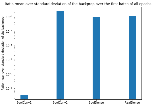
Figure 4: Empirical ratio of the mean to standard deviation of the backpropagation signal, experimented with CNN composed of BoolConv - BoolConv - BoolDense - RealDense layers and MNIST dataset.

It follows that:

$$Z^{l}\sim\mathcal{N}(\mu,\sigma^{2}),\quad\textrm{with }\quad\mu\ll\sigma.$$ (25)

We also assume that signals are mutually independent, i.e., computations are going to be made on random vectors, matrices and tensors, and it is assumed that the coefficients of these vectors, matrices and tensors are mutually independent. We assume that forward signals, backpropagation signals, and weights (and biases) of the layers involved are independent.

Consider a Boolean linear layer of input size $n$ and output size $m$, denote:

• Boolean weights: $W^{l}\in\mathbb{B}^{m\times n}$;

• Boolean inputs: $X^{l}\in\mathbb{B}^{n}$;

• Pre-activation and Outputs: $S^{l}\in[|-n,n|]^{m}$, $X^{l+1}\in\mathbb{B}^{m}$;

• Downstream backpropagated signal: $Z^{l}\in\mathbb{R}^{m}$;

• Upstream backpropagated signal: $Z^{l-1}\in\mathbb{R}^{n}$.

In the forward pass, we have: $S^{l}=\mathbf{xor}(W^{l},X^{l})$, and $X^{l+1}=\mathbf{maj}(S^{l})$.

With the following notations:

• $W^{l}=(W^{l}_{ij})_{i<m,j<n}\sim(\mathbf{B}(p_{ij}))_{i<m,j<n}$ with $p_{ij}\in[0,1]$;

• $X^{l}=(X^{l}_{i})_{i<n}\sim(\mathbf{B}(q_{i}))_{i<n}$ with $q_{i}\in[0,1]$;

• $Z^{l}=(Z^{l}_{i})_{i<m}\sim(\mathcal{N}(\mu_{i},\sigma_{i}^{2}))_{i<m}$;

• $\tilde{Z}$ stands for the truncated (with derivative of tanh) version of $Z$ for sake of simplicity.

And assuming that $\forall i,\sigma_{i}=\sigma,\mu_{i}=\mu$ and $\mu\ll\sigma$, we can derive scaling factors for linear layers in the next paragraph.

Remark C.1.

The scaling factor inside a convolutional layer behaves in a similar fashion except that the scalar dot product is replace by a full convolution with the 180-rotated kernel matrix.

C.3 Pre-Activation Scaling

We start by computing the variance of the pre-activation signal $S^{l}$ with respect to the number of neurons, without considering the influence of backward $\operatorname{tanh}^{\prime}$:

$$\forall j<n,\operatorname{Var}(S^{l}_{j}) =\sum_{i}^{m}\operatorname{Var}(W^{l}_{ij}X^{l}_{i}),\quad\text{($W$, $X$ are self mutually independent)}$$ (26)

$$=\sum_{i}^{m}\mathbb{E}\left[{W^{l}_{ij}}^{2}{X^{l}_{i}}^{2}\right]-\mathbb{E}\left[W^{l}_{ij}X^{l}_{i}]^{2}\right]$$ (27)

$$=\sum_{i}^{m}\mathbb{E}\left[{W^{l}_{ij}}^{2}\right]\mathbb{E}\left[{X^{l}_{i}}^{2}\right]-\mathbb{E}\left[W^{l}_{ij}\right]^{2}\mathbb{E}\left[X^{l}_{i}\right]^{2},\quad\text{($W$, $X$ are independent)}$$ (28)

$$=\sum_{i}^{m}\mathbb{E}\left[{X^{l}_{i}}^{2}\right]-(2p_{ij}-1)^{2}\mathbb{E}\left[X^{l}_{i}\right]^{2}$$ (29)

$$\simeq m\mathbb{E}\left[{X^{l}}^{2}\right],\qquad\text{since $\mu\ll\sigma$}$$ (30)

$$=m.$$ (31)

This leads to $\alpha=\nicefrac{{\pi}}{{2\sqrt{3m}}}$ in order to have $\operatorname{Var}(\alpha S)=\nicefrac{{\pi^{2}}}{{12}}$. This scaling allows one to match the distribution of any pre-activation signal $S$ with the $\operatorname{tanh}$ derivative one.

C.4 Backpropagation Scaling

We now compute the variance of the upstream backpropagated signal $Z^{l-1}$ with respect to the number of neurons and the variance of the downstream backpropagated signal:

$$\forall j<n,\operatorname{Var}(Z^{l-1}_{j}) =\sum_{i}^{m}\operatorname{Var}(W^{l}_{ij}\tilde{Z}^{l}_{i}),\quad\text{($W$, $Z$ are self mutually independent)}$$ (32)

$$=\sum_{i}^{m}\mathbb{E}\left[{W^{l}_{ij}}^{2}\tilde{Z^{l}_{i}}^{2}\right]-\mathbb{E}\left[W^{l}_{ij}\tilde{Z}^{l}_{i}\right]^{2}$$ (33)

$$=\sum_{i}^{m}\mathbb{E}\left[{W^{l}_{ij}}^{2}\right]\mathbb{E}\left[\tilde{Z^{l}_{i}}^{2}\right]-\mathbb{E}\left[W^{l}_{ij}\right]^{2}\mathbb{E}\left[\tilde{Z}^{l}_{i}\right]^{2},\quad\text{($W$, $Z$ are independent)}$$ (34)

$$=\sum_{i}^{m}\mathbb{E}\left[\tilde{Z^{l}_{i}}^{2}\right]-(2p_{ij}-1)^{2}\mathbb{E}\left[\tilde{Z}^{l}_{i}\right]^{2}$$ (35)

$$\simeq m\mathbb{E}\left[\tilde{Z^{l}}^{2}\right],\qquad\qquad\qquad\qquad\qquad\qquad\qquad\text{($\mu\ll\sigma)$}$$ (36)

$$=m\mathbb{E}\left[{Z^{l}}^{2}\right]\mathbb{E}\left[\frac{\partial\operatorname{tanh}}{\partial u}(u=\alpha W^{l}\cdot x^{l})^{2}\right],\qquad\text{(independence assump.)}$$ (37)

Let us focus on the term $\mathbb{E}\left[\frac{\partial\operatorname{tanh}}{\partial u}(u)^{2}\right]$, where $u\in[|-m,m|]$ for m even. The probability $\mathbb{P}(u=l)$ is computed thanks to enumeration. The event “$u=l$” indicates that we have $k+l$ scalar values at level “$+1$” and $k$ at level “$-1$” such that $2k+l=m$. Hence,

$$\mathbb{P}(u=l)=\binom{m}{\frac{m-l}{2}}\frac{1}{2}^{\frac{m-l}{2}}\frac{1}{2}^{m-\frac{m-l}{2}}.$$ (38)

Thus,

$$\mathbb{E}\left[\frac{\partial\operatorname{tanh}}{\partial u}(u)^{2}\right] =\sum_{u=-m}^{m}\frac{\partial\operatorname{tanh}}{\partial u}(u)^{2}p(u)$$ (39)

$$=2\sum_{u=0}^{m}\frac{\partial\operatorname{tanh}}{\partial u}(u)^{2}p(u),\qquad\text{(with symmetry)}$$ (40)

$$=\frac{1}{2^{m-1}}\sum_{u=0,u\;even}^{m}\binom{m}{\frac{m-l}{2}}(1-\operatorname{tanh}^{2}(\alpha u)).$$ (41)

The latter can be easily pre-computed for a given value of output layer size $m$, see Figure5.

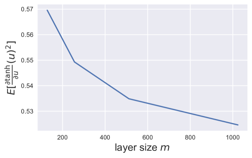
Figure 5: Expected value of $\operatorname{tanh}$ derivative with integer values as input, for several output sizes $m$.

The above figure suggests that for reasonable layer sizes $m$, $\mathbb{E}\left[\frac{\partial\operatorname{tanh}}{\partial u}(u=\alpha W^{l}\cdot x^{l})^{2}\right]\simeq\frac{1}{2}$. As a consequence we can make use of (37), and approximate the variance of the backpropagated signal as:

$$\operatorname{Var}(Z^{l-1})=\frac{m}{2}\operatorname{Var}(Z^{l}).$$ (42)

Remark C.2.

The backpropagation inside a convolutional layer behaves in a similar fashion except that the tensor dot product is replace by a full convolution with the 180-rotated kernel matrix. For a given stride $v$ and kernel sizes $k_{x},k_{y}$, the variance of the backpropagated signal is affected as follow:

$$\operatorname{Var}(Z^{l-1})=\frac{mk_{x}k_{y}}{2v}\operatorname{Var}(Z^{l}).$$ (43)

Let denote by MP the maxpooling operator (we assume its size to be $(2,2)$). In the backward pass, one should not forget the impact of the $\operatorname{tanh}^{\prime}(\alpha\Delta)$, and the MP operator so that:

$$Z^{l-1}=\mathrm{Conv}_{\mathrm{full}}\left(W_{\textrm{rot180}}^{l},Z^{l}\right)\cdot\frac{\partial\operatorname{tanh}}{\partial u}(u=\mathrm{MP}[\mathrm{Conv}(\alpha W^{l},X^{l})])\cdot\frac{\partial\mathrm{MP}}{\partial u}(u=\mathrm{Conv}(\alpha W^{l},X^{l})).$$ (44)

Let us focus on the last term: $\frac{\partial\mathrm{MP}}{\partial u}(u=\mathrm{Conv}(\alpha W^{l},X^{l}))=\mathbf{1}\left(u=\max(\mathrm{Conv}(\alpha W^{l},X^{l}))\right)$. Hence,

$$\mathbb{E}\left[\frac{\partial\mathrm{MP}}{\partial u}(u=\mathrm{Conv}(\alpha W^{l},X^{l}))^{2}\right] =\mathbb{E}\left[\frac{\partial\mathrm{MP}}{\partial u}(u=\mathrm{Conv}(\alpha W^{l},X^{l}))\right]$$ (45)

$$=\frac{1}{4}\times 1+0.$$ (46)

As a consequence, for a given stride $v$ and kernel sizes $k_{x},k_{y}$, the variance of the backpropagated signal is affected as follow:

$$\operatorname{Var}(Z^{l-1})=\frac{1}{4}\frac{mk_{x}k_{y}}{2v}\operatorname{Var}(Z^{l}).$$ (47)

Appendix D Experimental Details

D.1 Image Classification

D.1.1 Training Setup

The presented methodology and the architecture of the described Boolean nns were implemented in PyTorch [76] and trained on 8 Nvidia Tesla V100 GPUs. The networks thought predominantly Boolean, also contain a fraction of fp parameters that were optimized using the Adam optimizer [53] with learning rate $10^{-3}$. For learning the Boolean parameters we used the Boolean optimizer (see Algorithm 8). Training the Boolean networks for image classification was conducted with learning rates $\eta=150$ and $\eta=12$ (see Equation 10), for architectures with and without batch normalization, respectively. The hyper-parameters were chosen by grid search using the validation data. During the experiments, both optimizers used the cosine scheduler iterating over 300 epochs.

We employ data augmentation techniques when training low bitwidth models which otherwise would overfit with standard techniques. In addition to techniques like random resize crop or random horizontal flip, we used RandAugment, lighting [67] and Mixup [110]. Following [94], we used different resolutions for the training and validation sets. For imagenet, the training images were 192$\times$192 px and 224$\times$224 px for validation images. The batch size was 300 for both sets and the cross-entropy loss was used during training.

D.1.2 cifar10

vgg-small is found in the literature with different fully-connected fully-connected (fc) layers. Several works take inspiration from the classic work of [24], which uses 3 fc layers. Since other bnn methodologies only use a single fc layer, Table 9 presents the results with the modified vgg-small.

Table 9: Top-1 accuracy for different binary methodologies using the modified vgg-small (ending with 1 fc layer) on the cifar10 dataset.

Method	Forward	Training	Acc.
	Bit-width (W/A)	Bit-width (W/G)	(%)
fp	$32/32$	$32/32$	93.8
xnor-net [82]	$1/1$	$32/32$	87.4
lab [43]	$1/1$	$32/32$	87.7
rad [27]	$1/1$	$32/32$	90.0
ir-net [80]	$1/1$	$32/32$	90.4
rbnn [64]	$1/1$	$32/32$	91.3
slb [106]	$1/1$	$32/32$	92.0
b$\oplus$ld [Ours]	$1/1$	$1/16$	90.8

D.1.3 Ablation Study on Image Classification

The final block design for image classification was established after iterating over two models. The Boolean blocks examined were evaluated using the resnet18 baseline architecture and adjusting the training settings to improve performance. Figure 6 presents the preliminary designs.

The Boolean Block I, Figure 6(a), is similar to the original resnet18 block in that bn operations are removed and ReLUs are replaced by the Boolean activation. This design always includes a convolution in the shortcut with spatial resolution being handled by the stride. Notice that for this block we add a Boolean activation after the Maxpool module in the baseline (also for the final baseline architecture). The Boolean Block II, Figure 6(b), is composed by two stacked residual modules. For downsampling blocks we use the reshaping operation to reduce the spatial resolution and enlarge the channel dimensions both by a factor of 2. The shortcut is modified accordingly with different operations in order to guarantee similar spatial dimensions before the summation.

(a) Boolean block I.

(b) Boolean block II.

(c) resnet18 layout.

Figure 6: Preliminary designs for the baseline architecture and the Boolean basic blocks. The dashed and red-shaded operations in the Boolean block II are introduced for downsampling blocks.

Table 10 summarizes the results obtained with the proposed designs on imagenet. During our experimentation, we validated the hypothesis that increasing network capacity on the convolutional layers yielded higher accuracy values. However, similar to fp cnns, we confirmed there is a limit by which the hypothesis ceases to be true, leading to overfitting. Incorporating a more severe training strategy had a sustained positive impact. Even so, for larger configurations, the compromise between accuracy and size can be cumbersome.

Among the strategies to reduce overfitting during training we included: mixup data-augmentation [110], image illumination tweaking, rand-augment and smaller input resolution for training than for validation [94]. All combined, increased the accuracy by $\sim$3 points (check results for Block II + base channel 230 with and w/o additional data augmentation).

Table 10: Evaluation of the proposed blocks in imagenet and their respective configurations during training.

Block	Base	$1^{st}$ Conv.	Shortcut	Data	Acc.
Design	Channel	Bit-width	Fil. Size	Augmentation	(%)
Block I	128	32	$1\times 1$	Random Crop, Random Flip	53.35
	192	32	$1\times 1$	Random Crop, Random Flip	56.79
	192	32	$1\times 1$	Lighting, Mixup, RandAugment and [94]	61.90
	256	32	$1\times 1$	Lighting, Mixup, RandAugment and [94]	64.32
	256	32	$3\times 3$	Lighting, Mixup, RandAugment and [94]	66.89
Block II	128	1	$1\times 1$	Random Crop, Random Flip	56.05
	128	32	$1\times 1$	Random Crop, Random Flip	58.38
	192	32	$1\times 1$	Random Crop, Random Flip	61.10
	192	32	$1\times 1$	Lighting, Mixup, RandAugment and [94]	63.21
	230	32	$1\times 1$	Random Crop, Random Flip	61.22
	230	32	$1\times 1$	Lighting, Mixup, RandAugment and [94]	64.41

Compared to Block II, notice that the data streams in Block I are predominantly Boolean throughout the design. This is because it makes use of lightweight data types such as integer (after convolutions) and binary (after activations). In addition, it avoids the need of using a spatial transformation that may affect the data type and data distribution. In that regard, Block II requires 4 times more parameters for the convolution after reshaping, than the corresponding operation in Block I. This is exacerbated in upper layer convolutions, where the feature maps are deeper. Therefore, it makes sense to use Block I, as it is lighter and less prone to overfitting when the network capacity is expanded.

D.1.4 Neural Gradient Quantization

For completeness, we also implemented neural gradient quantization to quantize it by using int4 quantization with logarithmic round-to-nearest approach [21] and statistics aware weight binning [22]. Statistics aware weight binning is a method that seeks for the optimal scaling factor, per layer, that minimizes the quantization error based on the statistical characteristics of neural gradients. It involves per layer additional computational computations, but stays negligible with respect to other (convolution) operations. On imagenet, we recover the findings from [21]: 4 bits quantization is enough to recover standard backpropagation performances.

D.1.5 Basic Blocks SOTA BNNs for Classification

Recent bnn methodologies have proposed different mechanisms to improve performance. Most of them exploit full-precision operations to adjust datastreams within the network, like shift and scaling factors before binary activations [67] or channel scaling through Squeeze-and-Excitation modules [72, 36]. Figure 7 shows the basic blocks of three methodologies that perform particularly well in imagenet. Together with bn and regular activations, those techniques not only add an additional level of complexity but also lead to heavier use of computational resources and latency delays.

For comparison we also show the proposed block (Figure 7(a)) used in our experiments for Image Classification, Image Segmentation and Image Super-Resolution. Our block is compact in the sense that it only includes Boolean convolutions and Boolean activations, strategically placed to keep the input and output datastreams Boolean.

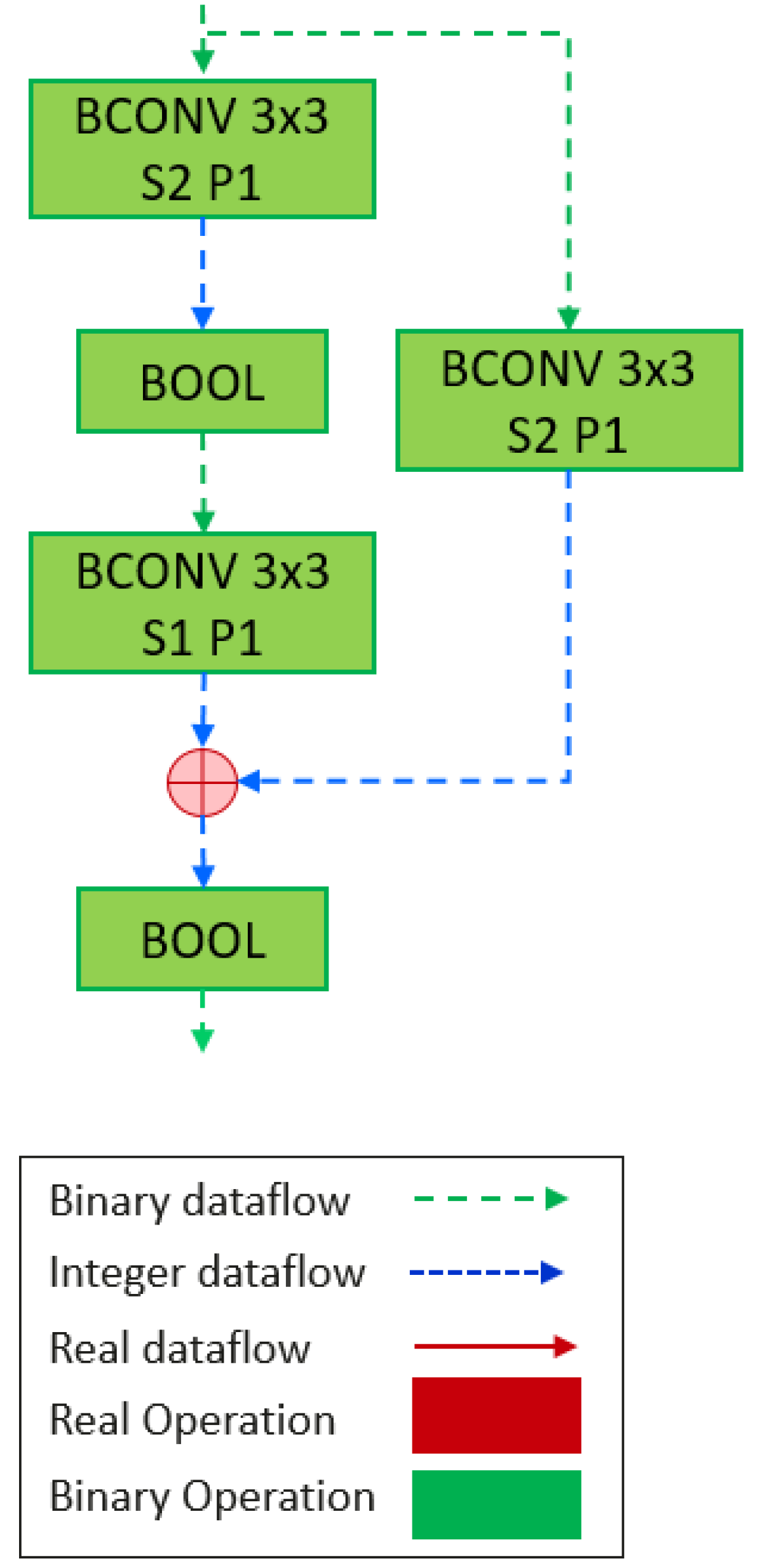
(a) Boolean Block w/o bn.

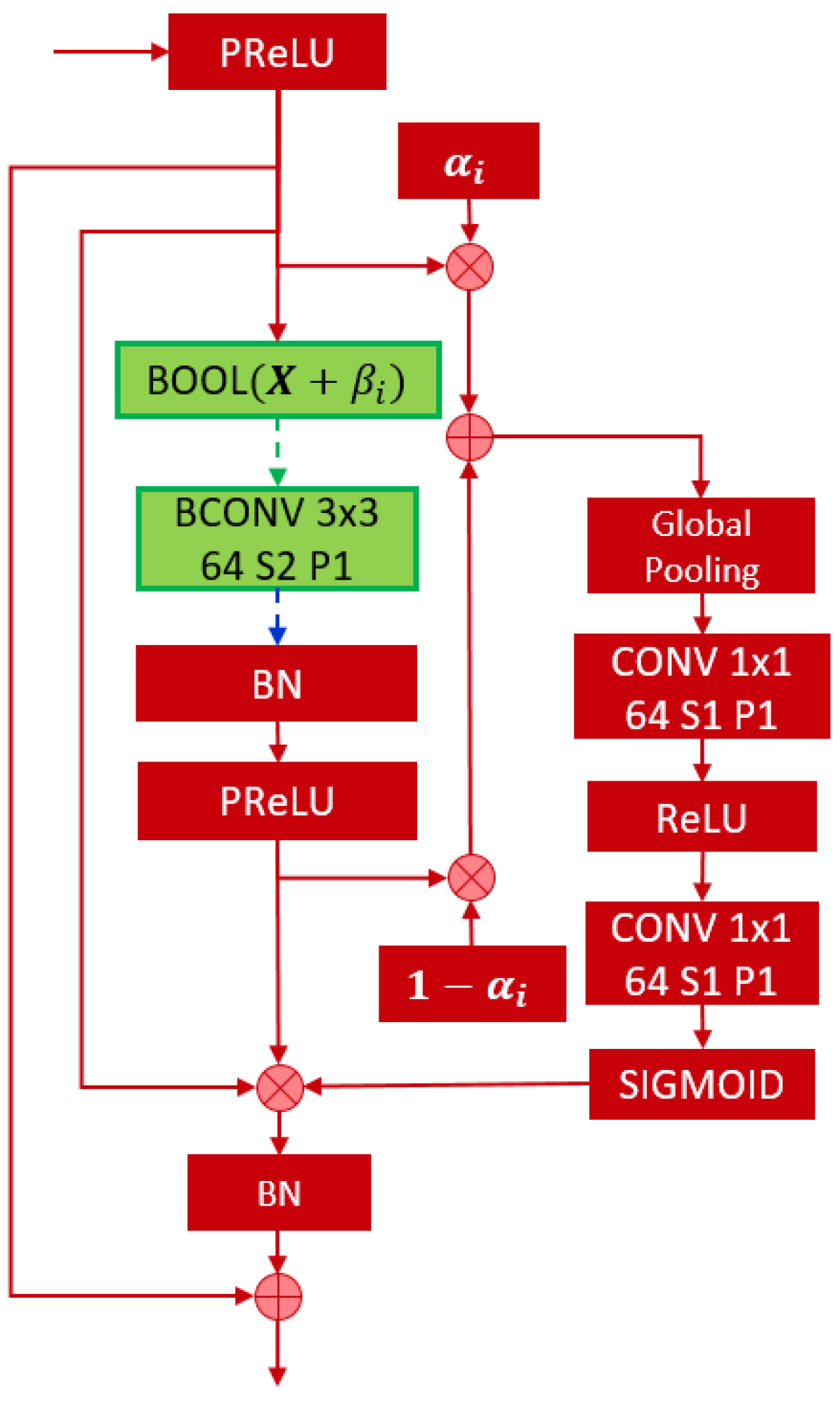
(b) bnext sub-block [36].

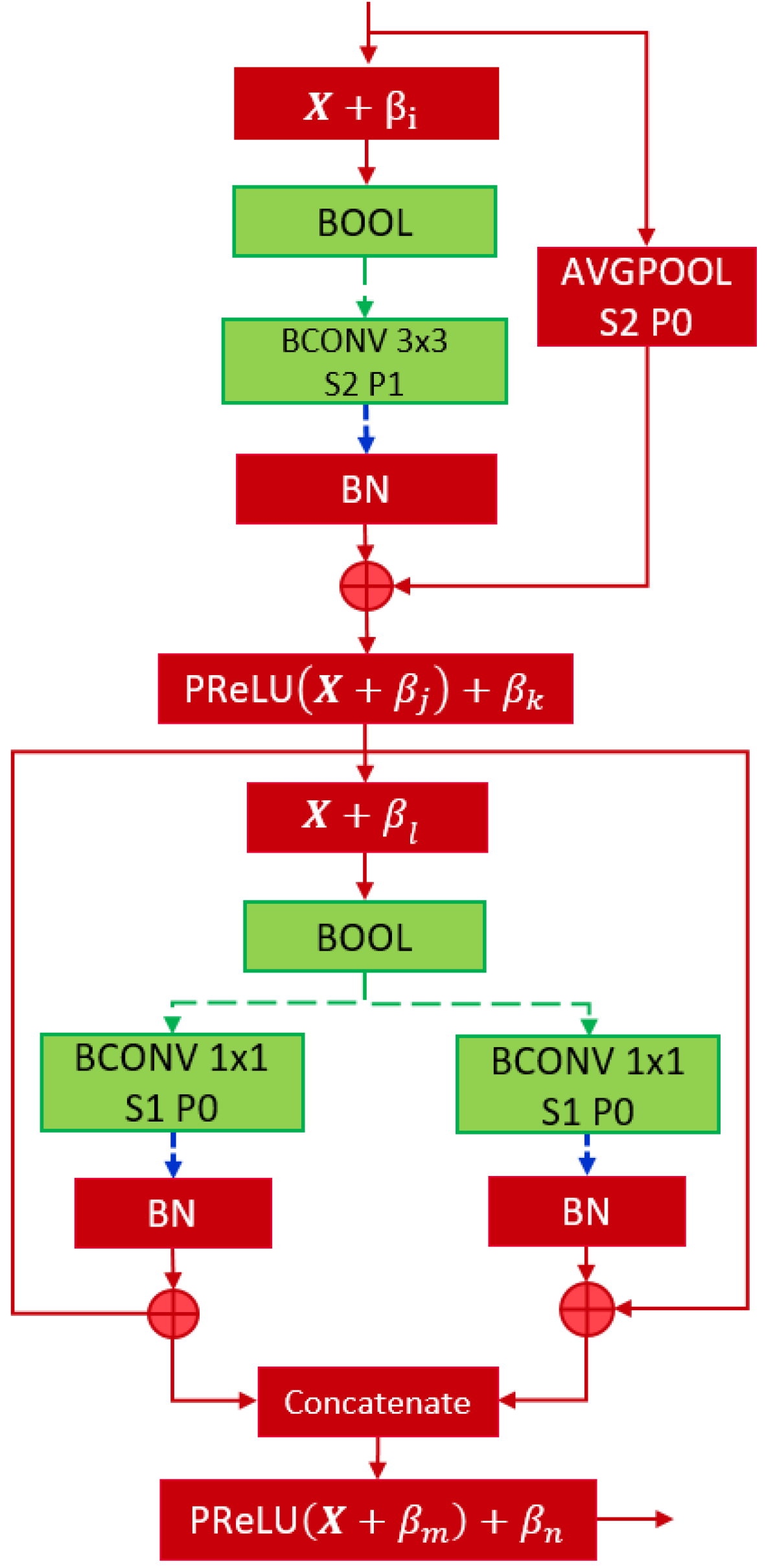
(c) reactnet [67].

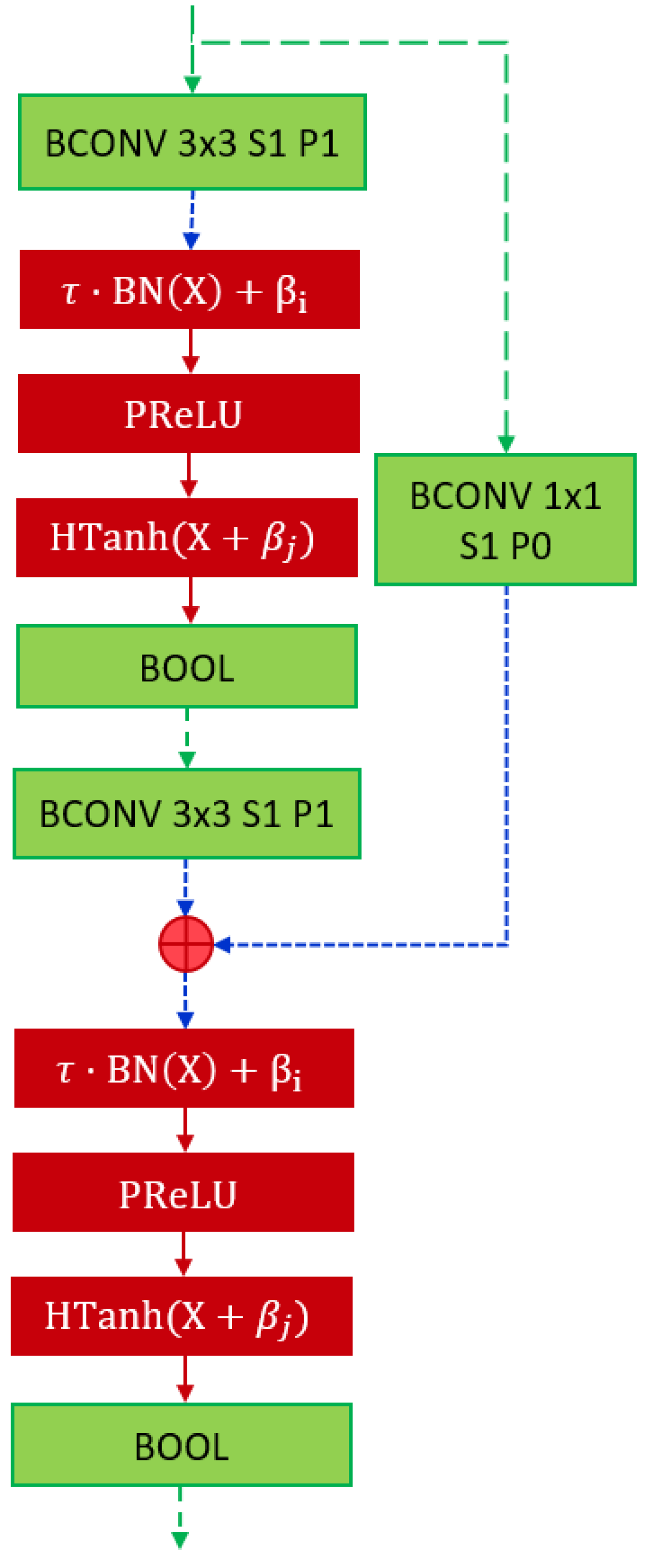
(d) bineal-net [75].

Figure 7: Comparative graph of popular bnn techniques and our Boolean module. Notice how multiple full-precision operations like bn, PReLU, or Squeeze-and-Excitation are overly used on each bnn block.

D.2 Image Super-resolution

The seminal edsr [63] method for super-resolution was used together with our Boolean methodology. In particular, the residual blocks are directly replaced by our Boolean basic block, see Figure 8. For all three tasks in super-resolution, (i.e. $\times 2$, $\times 3$, $\times 4$), training was carried out with small patches of 96$\times$96 px (40 of them extracted randomly from each single image in the div2k dataset) and validated with the original full-resolution images. The learning rate for real and boolean parameters were $10^{-4}$ and $\eta=36$, respectively. The networks were trained by minimizing the $L_{1}$-norm between the ground-truth and the predicted upsampled image while using the Adam optimizer and Boolean optimizer (see Algorithm 8). In our experiments the batch size was 20. Some example images generated by our methodology are showed in Figures 9 and 10.

(a) Small edsr .

(b) Our Boolean edsr.

Figure 8: Small edsr for single scale $\times 2$ super-resolution and our Boolean version with Boolean residual blocks. In both architectures the channels dimensions are $\kappa=256$ and the shaded blocks are repeated $8\times$.

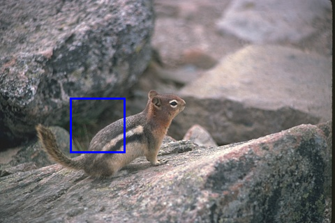
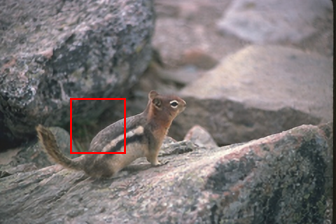
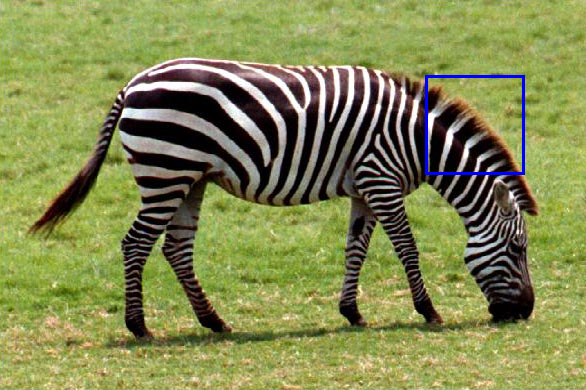
(a) Ground-truth targets.

(b) Enlarged crops.

(c) Predicted images.

(d) Enlarged crops.

Figure 9: Ground-truth high resolution images and the output of our Boolean super-resolution methodology. First row: image “013” from bsd100, with PSNR: 35.54 dB. Second row: image “014” from Set14, with PSNR: 33.92 dB.

(a) Ground-truth target.

(b) Enlarged crop.

(c) Predicted image.

(d) Enlarged crop.

Figure 10: Ground-truth high resolution target image (top) and the output of our Boolean super-resolution methodology (bottom). Image “0810” from the validation set of div2k, with PSNR: 34.90 dB

D.3 Semantic Segmentation

D.3.1 Network architecture

Figure 11: Boolean segmentation architecture.

Our Boolean architecture is based on deeplabv3 [17], which has shown great success in semantic segmentation. It is proven that using dilated or atrous convolutions, which preserve the large feature maps, instead of strided convolutions is prominent for this task. In our Boolean model with resnet18 layout, we replace the strided convolutions in the last two resnet18 layers with the non-strided version, and the dilated convolutions are employed to compensate for the reduced receptive field. Thus, the images are $8\times$ downsampled instead of $32\times$, preserving small object features and allowing more information flow through the Boolean network. As shown in Figure 6(a), in the Boolean basic block, a $3\times 3$ convolution instead of $1\times 1$ convolution is used to ensure the comparable dynamic range of pre-activations between the main path and the shortcut. Keeping these Boolean convolutional layers non-dilated naturally allows the backbone to extract multi-scale features without introducing additional computational cost.

(a)

(b)

(c)

(d)

Figure 12: Boolean Atrous Spatial Pyramid Pooling (bool-aspp) architecture. (a) $1\times 1$ Conv branch. (b) $3\times 3$ dilated Conv branch with dilation rate of $d$. (c) Naive global average pooling branch. (d) Global average pooling branch.

The Atrous Spatial Pyramid Pooling (aspp) consists of multiple dilated convolution layers with different dilation rates and global average pooling in parallel, which effectively captures multi-scale information. In the Boolean aspp (bool-aspp), we use one $1\times 1$ Boolean convolution and three $3\times 3$ Boolean dilated convolution with dilation rates of $\{12,24,36\}$ following by Boolean activation functions. The global average pooling (gap) branch in aspp captures image-level features, which is crucial for global image understanding as well as large object segmenting accuracy. However, in bool-aspp, as shown in Figure 12(c), the Boolean input $X$ leads to significant information loss before the global average pooling may cause performance degradation on large objects. Therefore, we keep the inputs integer for the gap branch as demonstrated in Figure 12(d). To prevent numerical instability, batch normalization is used in the gap branch before each activation function. Using bool-aspp enhances the multi-scale feature extraction and avoids parameterized upsampling layers, e.g. transposed convolution.

D.3.2 Training setup

The model was trained on the cityscapes dataset for $400$ epochs with a batch size of $8$. The AdamW optimizer [70] with an initial learning rate of $5\times 10^{-4}$ and the Boolean logic optimizer (see Algorithm 8) with a learning rate of $\eta=12$ were used respectively for real and Boolean parameters. At the early training stage, parameters could easily be flipped due to the large backward signal; thus, to better benefit from the imagenet-pretrained backbone, we reduce the learning rate for Boolean parameters in the backbone to $\eta=6$. We employed the polynomial learning rate policy with $p=0.9$ for all parameters. The cross-entropy loss was used for optimization. We did not employ auxiliary loss or knowledge distillation as these training techniques require additional computational cost, which is not in line with our efficient on-device training objective.

D.3.3 Data sampling and augmentation

Table 11: Class per image and performance gap occurrence rates in cityscapes training set with naive bool-aspp design. Class with low performance gap^† and class with high performance gap^∗.

	Image ratio (%)	$\Delta$ mIoU (%)
Road†	$98.62$	$0.0$
Sideway†	$94.49$	$0.7$
Building†	$98.62$	$0.6$
Wall	$32.61$	$7.4$
Fence	$43.56$	$3.8$
Pole	$99.13$	$1.8$
Light	$55.73$	$6.5$
Sign†	$94.39$	$2.8$
Vegetation†	$97.18$	$0.1$
Terrain†	$55.60$	$0.8$
Sky†	$90.29$	$-0.2$
Person	$78.76$	$1.5$
Rider∗	$34.39$	$7.4$
Car†	$95.19$	$0.3$
Truck∗	$12.07$	$6.9$
Bus∗	$9.21$	$12.8$
Train∗	$4.77$	$17.0$
Motor∗	$17.24$	$15.3$
bike	$55.33$	$2.0$

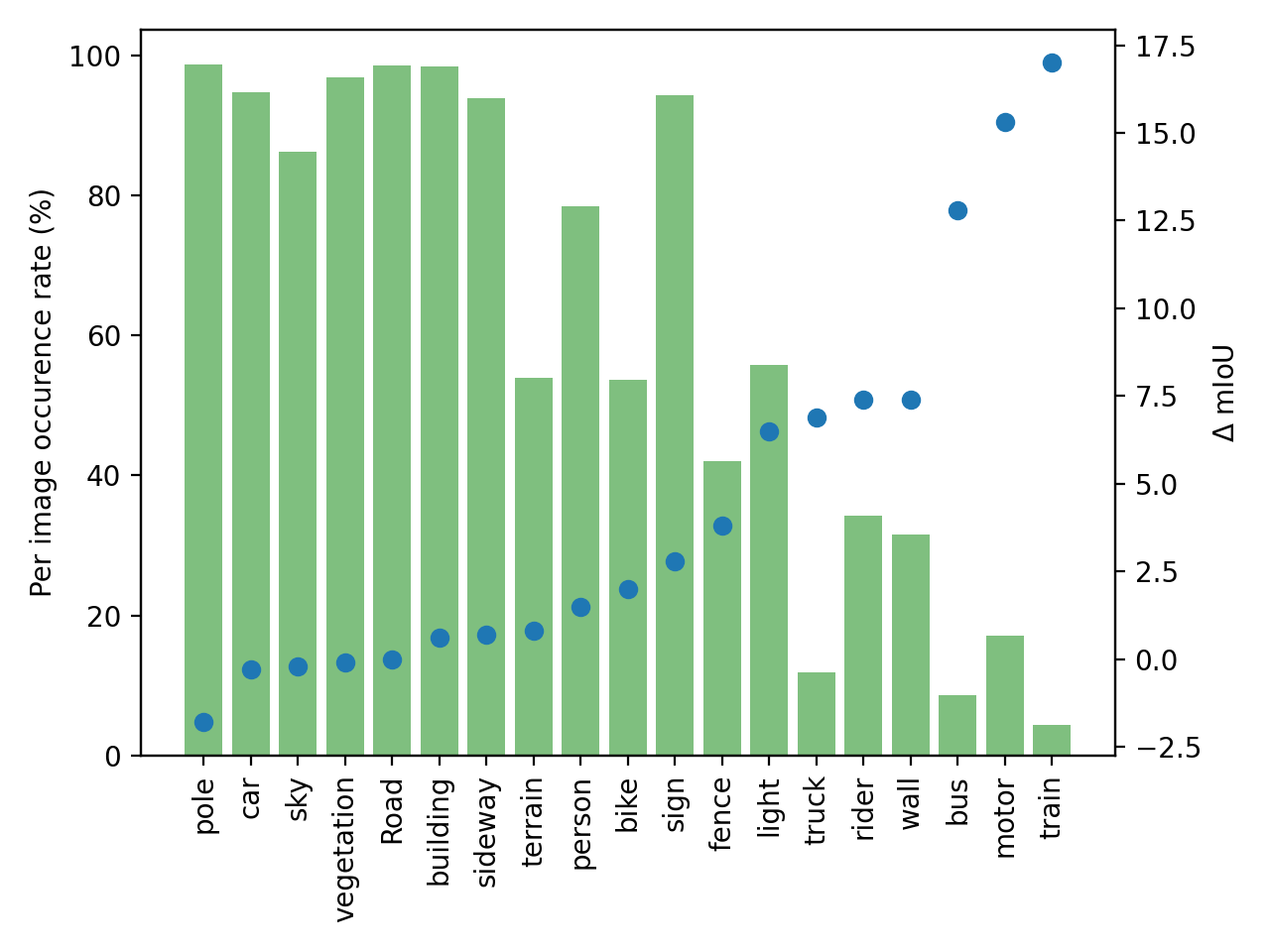
Figure 13: Class per image occurrence ratio and performance gap with naive bool-aspp design.

We aim to reproduce closely full-precision model performance in the semantic segmentation task with Boolean architecture and Boolean logic training. Due to the nature of the Boolean network, the common regularization method, e.g., weight decay, is not applicable. Moreover, with more trainable parameters, the Boolean network can suffer from over-fitting. In particular, as shown in Table 11, the imbalanced dataset for semantic segmentation aggravates the situation. There is a significant performance gap for several classes which has low occurrence rate, including rider (9.5%), motor (11.2%), bus (9.5%), truck (6.9%), train (17.0%). We argue that the performance gap is due to the similarity between classes and the dataset’s low occurrence rate, which is confirmed as shown in Figure 13.

Data augmentation and sampling are thus critical for Boolean model training. Regarding data augmentation, we employed multi-scale scaling with a random scaling factor ranging from $0.5$ to $2$. We adopted a random horizontal flip with probability $p=0.5$ and color jittering. In addition, we used rare class sampling (RCS) [45] to avoid the model over-fitting to frequent classes. For class $c$, the occurrence frequency in image $f_{c}$ is given by:

$$f_{c}=\frac{\sum_{i=1}^{N}\mathbf{1}\left(c\in y_{i}\right)}{N},$$ (48)

where $N$ is the number of samples and $y_{i}$ is the set of classes existing in sample $i$. The sampling probability of class $c$ is thus defined as:

$$p_{c}=\frac{\exp\left(\frac{1-f_{c}}{T}\right)}{\sum_{c^{\prime}=1}^{K}\exp\left(\frac{1-f_{c^{\prime}}}{T}\right)},$$ (49)

where $K$ is the number of classes, and $T$ is a hyper-parameter for sampling rate balancing. In particular, for the cityscapes dataset, we selected $T=0.5$.

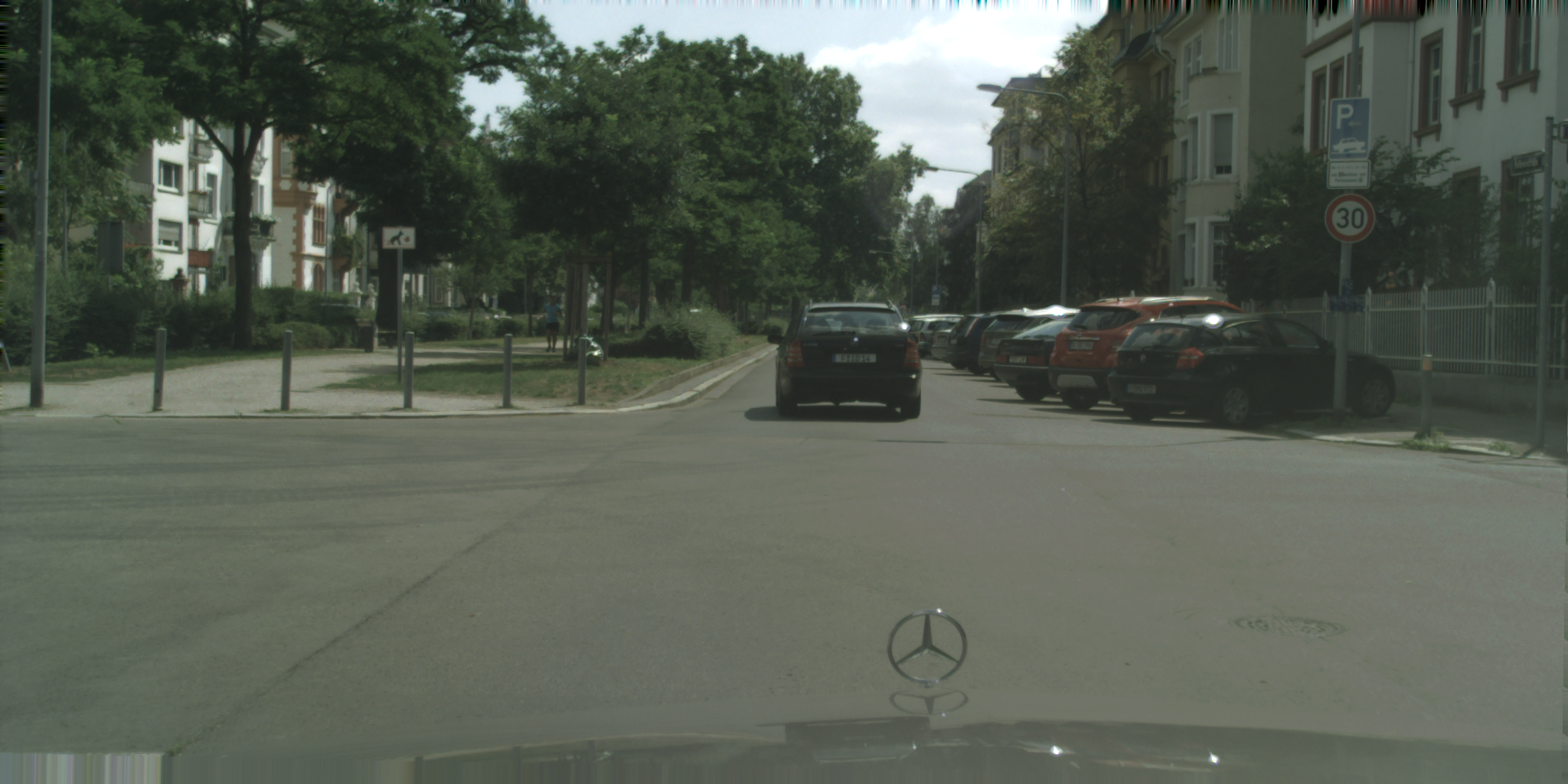
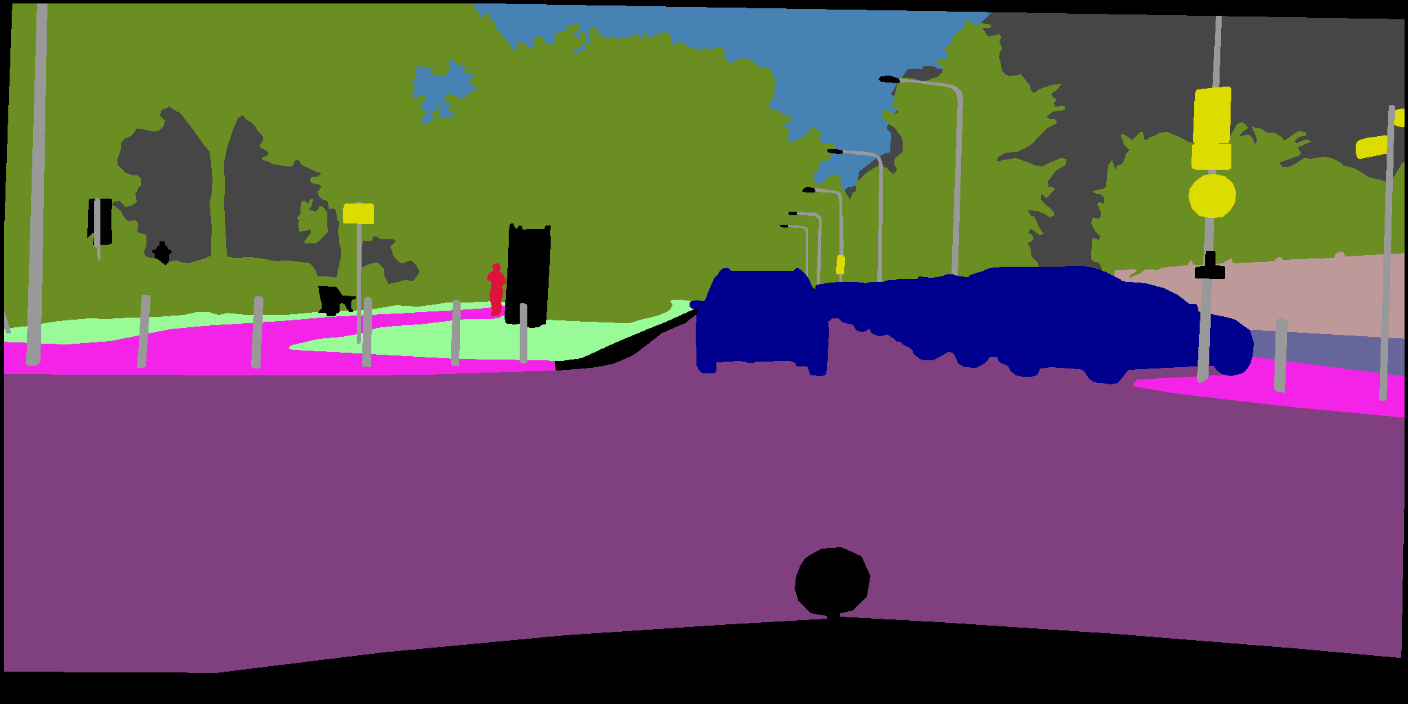
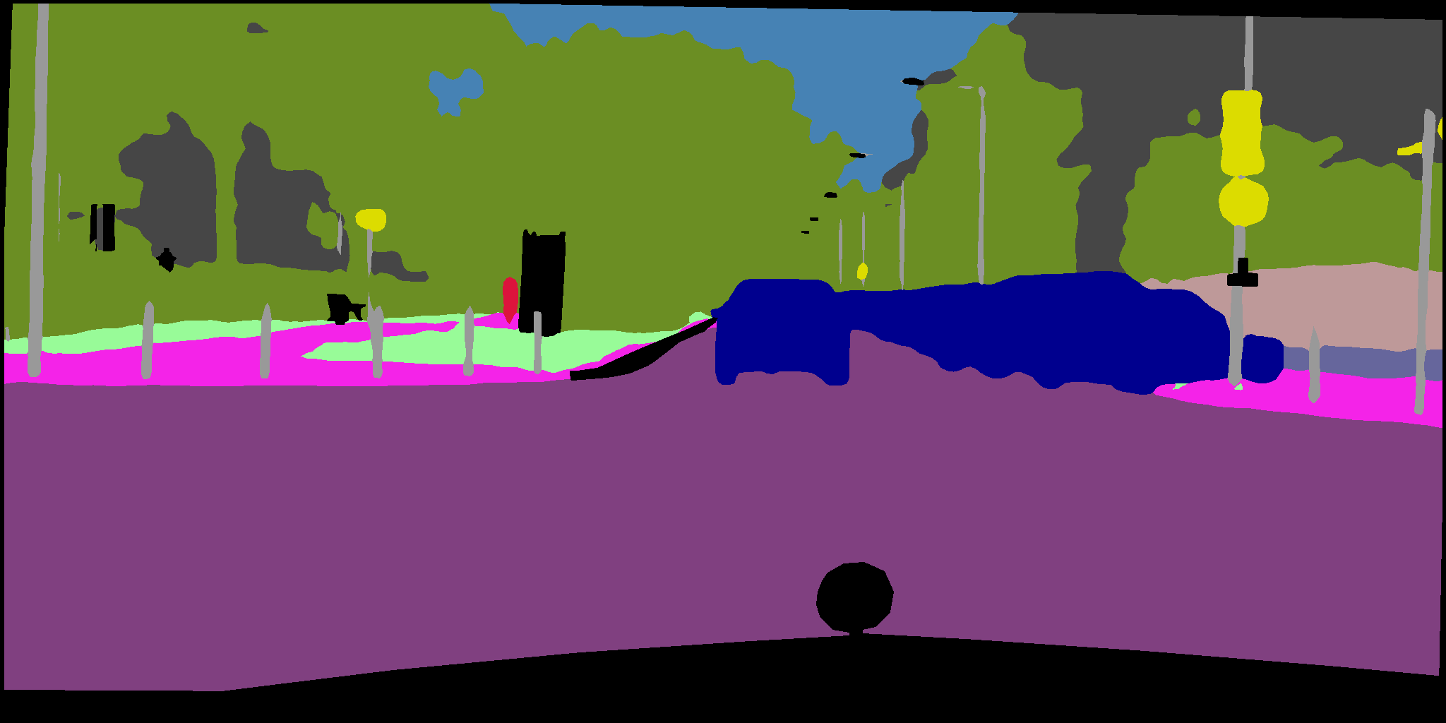
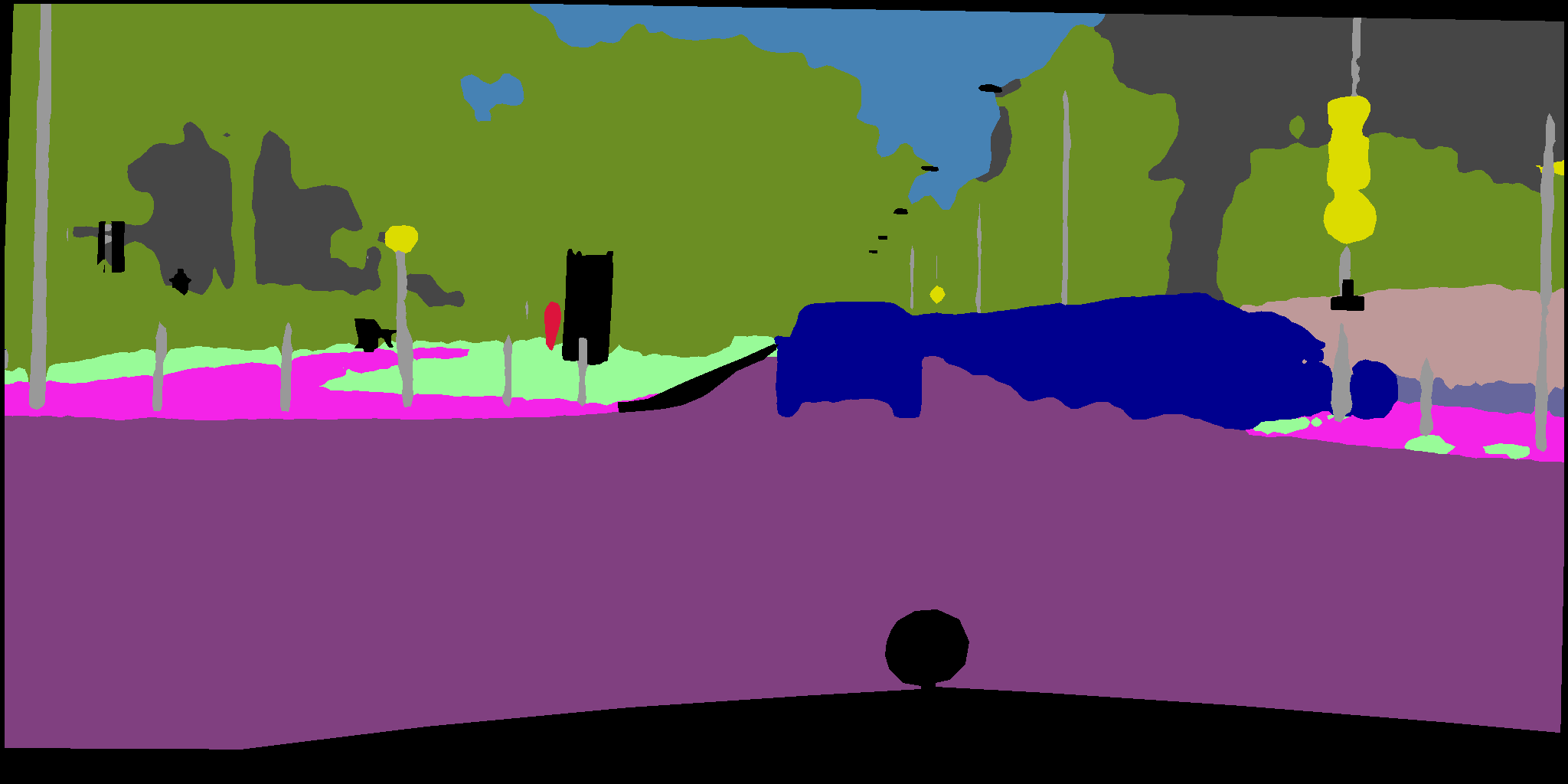
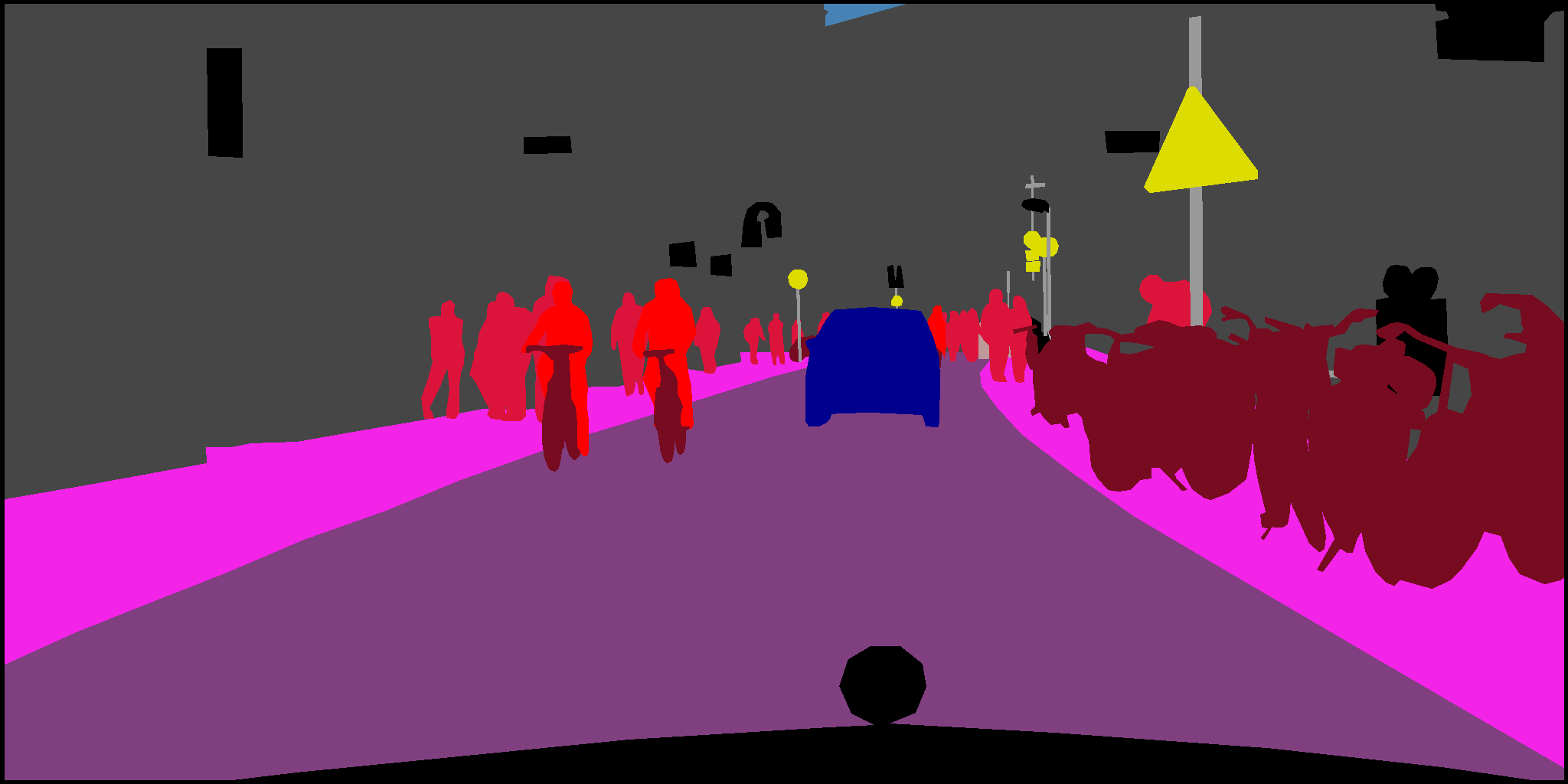
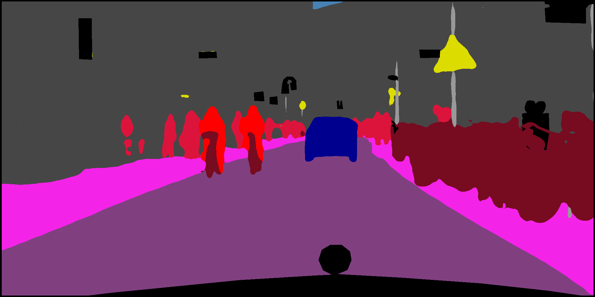
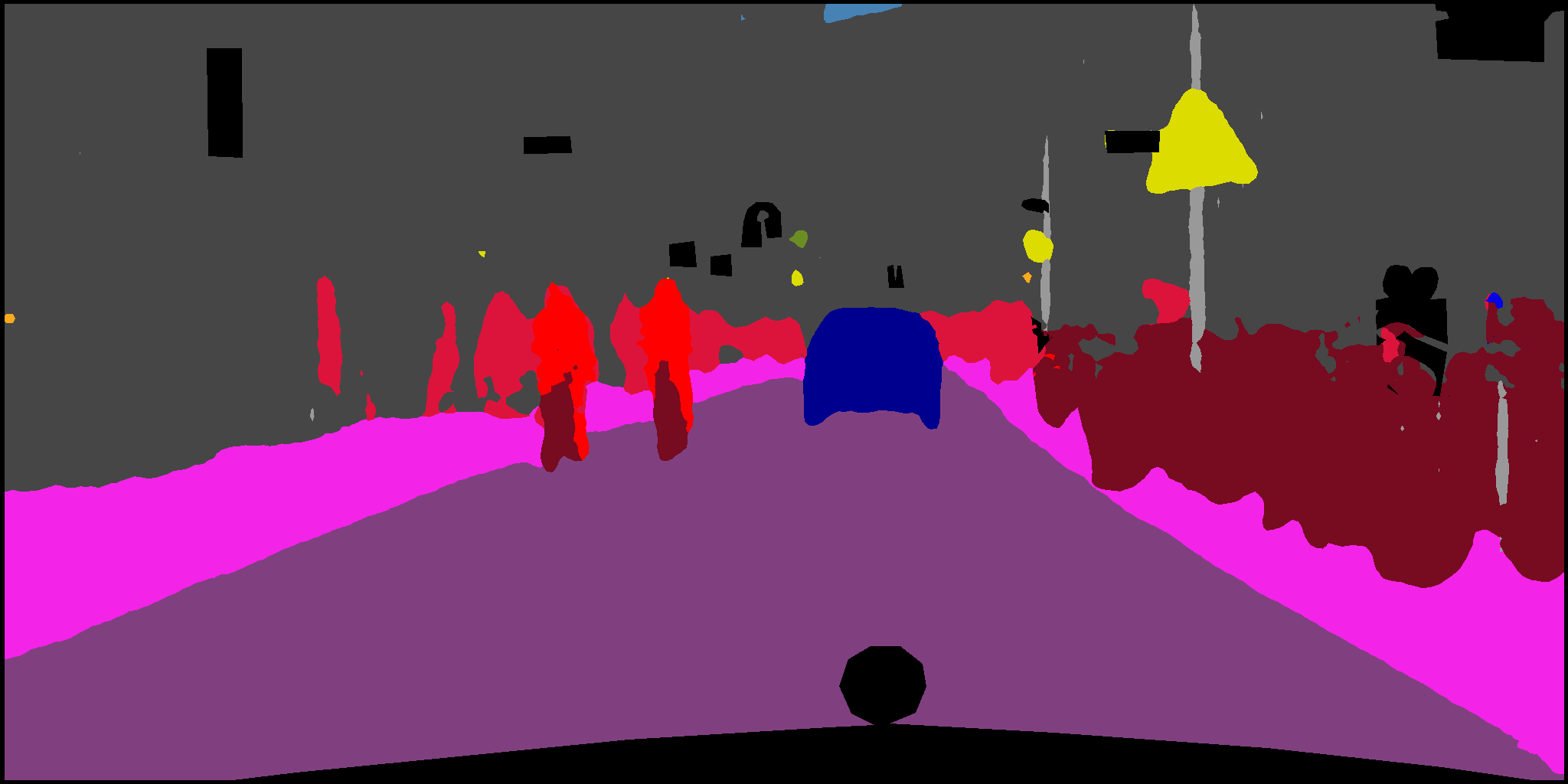
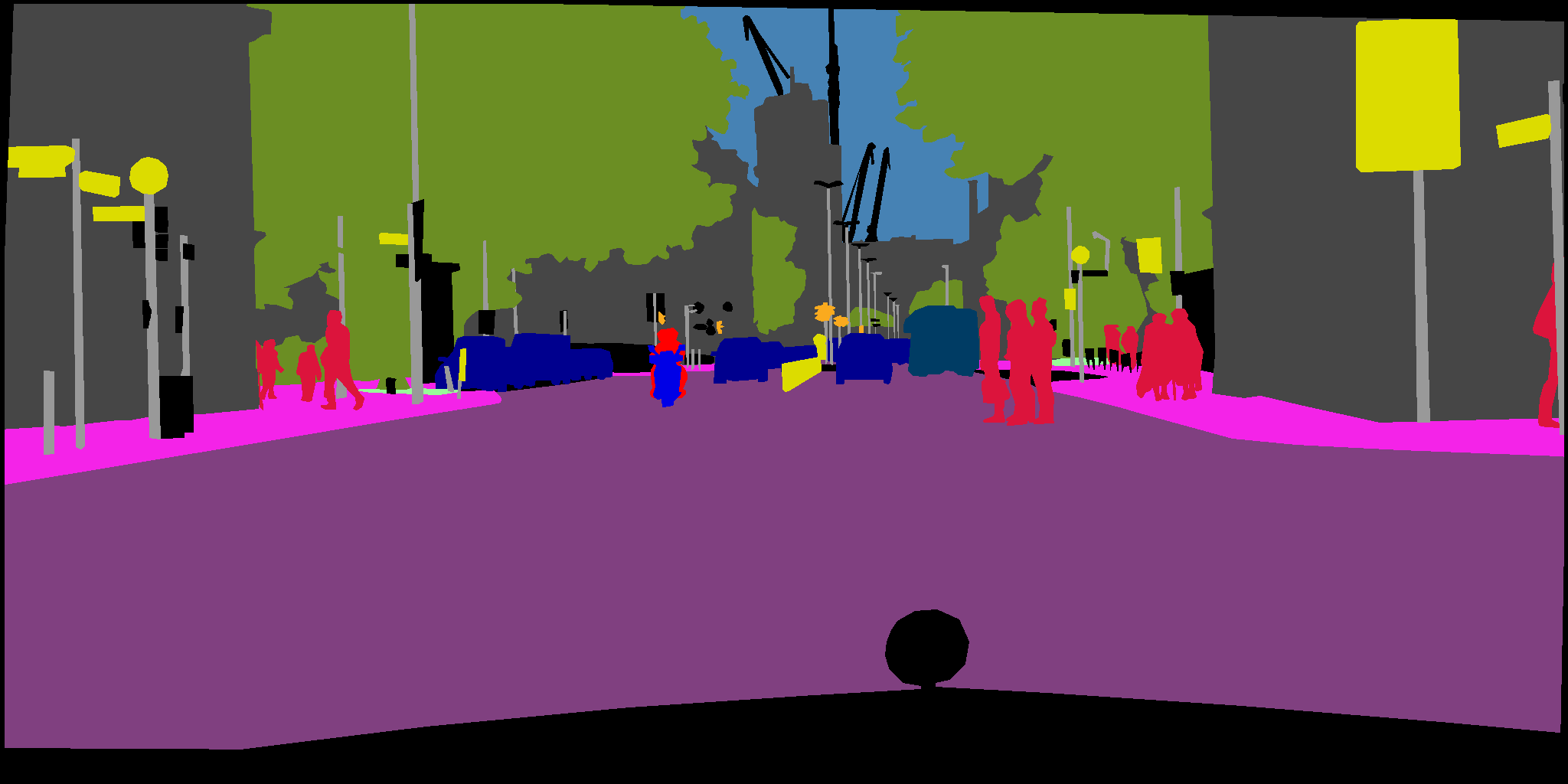
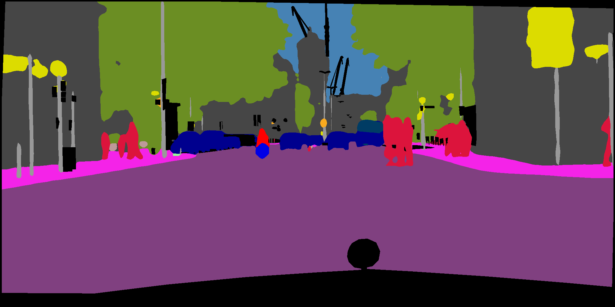
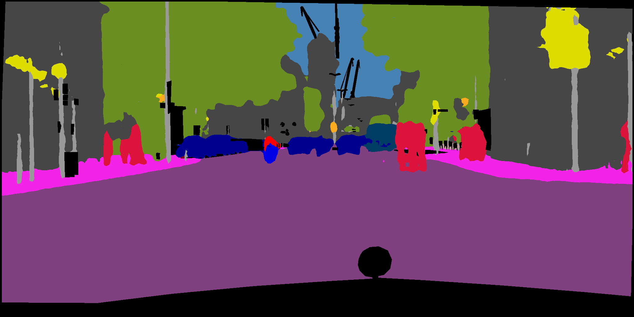
Input image

Ground truth

Full-precision

b$\oplus$ld (Ours)

Figure 14: Qualitative comparison of Boolean model on cityscapes validation set.

D.3.4 Qualitative analysis on cityscapes validation set

The qualitative results of our Boolean network and the full-precision based are demonstrated in Figure 14. Despite the loss of model capacity, the proposed Boolean network trained with Boolean logic optimizer has comparable performance with large objects in the frequent classes, even in the complicated scene.

D.3.5 More experiments on semantic segmentation

Table 12: Class-wise IoU performance on cityscapes validation set.

Methods	road	sideway	building	wall	fence	pole	light	sign	vegetation	terrain	sky	person	rider	car	truck	bus	train	motor	bike	mIoU
FP baseline	97.3	79.8	90.1	48.5	55.0	49.4	59.2	69.	90.0	57.5	92.4	74.3	54.6	91.2	61.4	78.3	66.6	58.0	70.8	70.7
Naive Bool ASPP	97.3	79.1	89.5	41.1	51.2	51.2	52.7	66.2	90.1	56.7	92.6	72.8	47.2	91.5	54.5	65.5	49.6	42.7	68.8	66.3
$\Delta$	0.0	0.7	0.6	7.4	3.8	-1.8	6.5	2.8	-0.1	0.8	-0.2	1.5	7.4	-0.3	6.9	12.8	17.0	15.3	2.0	4.4
b$\oplus$ld [Ours]	97.1	78.	89.8	46.2	51.3	52.7	53.3	66.5	90.2	58.	92.7	72.6	45.1	91.9	61.1	68.8	48.7	46.8	69.1	67.4
$\Delta$	0.2	1.8	0.3	2.3	3.7	-3.3	5.9	2.5	-0.2	-0.5	-0.3	1.7	9.5	-0.7	0.3	9.5	17.9	11.2	1.7	3.3

We evaluated the effectiveness of bool-aspp by investigating the per-class performance gap to the full-precision model. As demonstrated in Table 12, a significant gap exists between the Boolean architecture with naive bool-aspp design; i.e., using Boolean activations for aspp module as illustrated in Figure 12(c). However, the gap could be reduced by using bool-aspp and RCS. In particular, the bool-aspp improves the IoU of truck from $54.5\%$ to $64.1\%$ and bus from $65.5\%$ to $68.8\%$, bike from $68.8\%$ to $69.1\%$ and motor from $42.8\%$ to $46.8\%$. This indicates that combining proposed bool-aspp and RCS improves the model performance on low occurrence classes as well as similar classes with which are easy to be confused.

D.3.6 Validation on pascal voc 2012 dataset

We also evaluated our Boolean model on the $21$-class pascal voc 2012 dataset with augmented additional annotated data containing $10,582$, $1,449$, and $1,456$ images in training, validation, and test set, respectively. The same setting is used as in the experiments on the cityscapes dataset, except the model was trained for $60$ epochs.

As shown in Table 13, our model with fully Boolean logic training paradigm, i.e., without any additional intermediate latent weight, achieved comparable performance as the state-of-the-art latent-weight-based method. Our Boolean model improved performance by incorporating multi-resolution feature extraction modules to $67.3\%$ mIoU.

Table 13: Performance on pascal voc 2012 val set.

Seg. head	Model	mIoU (%)	$\Delta$
fcn-32s [69]	fp baseline	64.9	-
	group-net [114]	60.5	4.4
	b$\oplus$ld [Ours]	60.1	4.8
deeplabv3 [17]	fp baseline	72.1	-
	b$\oplus$ld [Ours]	67.3	4.8

D.4 Boolean BERT Fine-tuning

We conducted experiments on the bert model [26] drawing on the experimental framework proposed in bit [66]. For this experiment, our goal was to fine-tune the original pre-trained bert model using Boolean precision. To validate our method we used the glue benchmark [98] with 8 datasets. For our experiments, we modified the baseline fp architecture using the proposed methodology Algorithm 8. That is, core operations within the transformer are substituted by native Boolean components, e.g. Boolean activations and Boolean linear layers. The fp parameters were optimized using the Adam optimizer with the learning rates proposed in [66]. Correspondingly for Boolean weights, we used our Boolean optimizer with learning rate $\eta=100$.

Appendix E Energy Estimation

Energy consumption is a fundamental metric for measuring hardware complexity. However, it requires specific knowledge of computing systems and makes it hard to estimate. Few results are available, though experimental-based and limited to specific tested models [see, e.g., 32, 84, 73, 12, 14, 33]. Although experimental evaluation is precise, it requires considerable implementation efforts while not generalizing. In addition, most relevant works are only limited to inference and not training [19, 56, 105].

E.1 Hardware Specification

Ascend architecture.

We intend to estimate the training energy consumption on Ascend chip architecture introduced in [62] and dedicated to DNN computing. The core design of Ascend is described in [62]. Essentially, it introduces a 3D (cube) computing unit, providing the bulk of high-intensity computation and increasing data reuse. On the other hand, it provides multiple levels of on-chip memory. In particular, memory L0, which is nearest to the computing cube, is tripled to boost further near-memory computing capability, namely L0-A dedicated to the left-hand-side (LHS) input data, L0-B dedicated to RHS input data, and L0-C for the output. For instance, in a convolution, L0-A, L0-B, and L0-C correspond to the input feature maps (ifmaps), filters, and output feature maps (ofmaps), respectively. In addition, the output results going through L0-C can be processed by a Vector Unit for in-place operations such as normalization and activation. Table 14 shows energy efficiency and capacity of the memory hierarchy of a commercial Ascend architecture [62].

Table 14: Memory hierarchy and energy efficiency (EE) of an Ascend core [62] used in our evaluation.

	L3 (DRAM)	L2	L1	L0-A	L0-B	L0-C
EE [GBPS/mW]	0.02	0.2	0.4	4.9	3.5	5.4
Capacity [KB]	$-$	8192	1024	64	64	256

Nvidia architecture.

We also have estimated the energy consumption for the Nvidia GPU (Tesla V100). Similarly, this architecture utilizes different memory levels with varying read and write energy characteristics. For instance, the L2 cache size is 6 MB per GPU. The L1 cache is 64 KB per Streaming Multiprocessor (SM). Each Tesla V100 GPU has 80 SMs, so the total L1 cache is 5120 KB (5 MB). However, specific details on the read and write energy consumption for each memory level of the Tesla V100 GPU are proprietary and not publicly disclosed by Nvidia. Thus, we show the normalized energy consumption relative to the computation of a MAC at the arithmetic logic unit (ALU). Table 15 shows the numbers for each storage level, which are extracted from a commercial 65 nm process [18].

Table 15: Normalized energy cost relative to the computation of one MAC operation at ALU.

DRAM	L2	L1	RF	1 MAC at ALU
$200\times$	$6\times$	$2\times$	$1\times$	$1\times$

E.2 Compute Energy

Energy consumption is the sum of compute and memory energies. Compute energy is simply given by the number of arithmetic operations multiplied by their unit cost. The number of arithmetic operations is directly determined from the layer’s parameters. For the Ascend architecture, their unit cost is obtained by considering the compute efficiency at 1.7 TOPS/W [62]. For Boolean logic operations, we follow the usual estimation that ADD INT-$n$ costs $(2n-1)$ logic operations where $n$ stands for bitwidth.

E.3 Memory Energy

On the other hand, memory energy is all consumed for moving data between their storage through memory levels and the computing unit during the entire lifetime of the process. Since energy consumed at each memory level is given by the number of data accesses to that level times per-access energy cost, it consists in determining the number of accesses to each level of all data streams (i.e., LHS, RHS, Output). Besides taking into account the hardware architecture and memory hierarchy of chip, our approach to quantifying memory energy is based on existing methods [19, 90, 56, 105, 42, 103] for dataflow and energy evaluation. Given the layer parameters and memory hierarchy, it amounts to:

1. Tiling: determining the tiling strategy for allocating data streams on each memory level.

2. Movement: specifying how data streams are reused or kept stationary to determine their access numbers.

In the following, we present our method for the forward and backward passes by taking the example of a convolution layer, as convolutions are the main components of cnns and the primary source of complexity due to their high data reuse. The parameters of 2D convolution layer are summarized in Table 16. Here, we denote ifmaps, filters, and ofmaps by $I$, $F$, and $O$, respectively.

Table 16: Shape parameters of a convolution layer.

Parameter	Description
$N$	batch size
$M$	number of ofmaps channels
$C$	number of ifmaps channels
$H^{I}/W^{I}$	ifmaps plane height/width
$H^{F}/W^{F}$	filters plane height/width
$H^{O}/W^{O}$	ofmaps plane height/width

E.3.1 Tiling

Since the ifmaps and filters are usually too large to be stored in buffers, the tiling strategy is aimed at efficiently transferring them to the computing unit. Determining tiling parameters, which are summarized in Table 17, is an NP-Hard problem [105].

Table 17: Tiling parameters of a convolution layer.

Parameter	Description
$M_{2}$	number of tiling weights in L2 buffer
$M_{1}$	number of tiling weights in L1 buffer
$M_{0}$	number of tiling weights in L0-B buffer
$N_{2}$	number of tiling ifmaps in L2 buffer
$N_{1}$	number of tiling ifmaps in L1 buffer
$N_{0}$	number of tiling ifmaps in L0-A buffer
$H^{I}_{2}/W^{I}_{2}$	height/width of tiling ifmaps in L2 buffer
$H^{I}_{1}/W^{I}_{1}$	height/width of tiling ifmaps in L2 buffer
$H^{I}_{0}/W^{I}_{0}$	height/width of tiling ifmaps in L0-A buffer

An iterative search over possibilities subject to memory capacity constraint provides tiling combinations of ifmaps and filters on each memory level. Different approaches can be used and Algorithm 9 shows an example that explores the best tiling parameters subjected to maximizing the buffer utilization and near compute stationary (i.e., as much reuse as possible to reduce the number of accesses to higher levels). Therein, the amount of data stored in level $\mathit{i}$ is calculated as:

$$Q^{I}_{i} =N_{i}\times C_{i}\times H^{I}_{i}\times W^{I}_{i}\times b^{I},$$ (50)

$$Q^{F}_{i} =M_{i}\times C_{i}\times H^{F}\times W^{F}\times b^{F},$$

where $Q^{I}_{i}/Q^{F}_{i}$ and $b^{I}/b^{F}$ represent the memory and bitwidth of ifmaps/filters, respectively.

Input: tiling parameters of ifmaps and filters at level $i+1$, and buffer capacity of level $i$.

Output: tiling parameters of ifmaps and filters at level $i$.

1 Initialize

2      $\mathcal{E}^{\textrm{min}}:=\infty$;

3 end

4

5for $M_{i}\leftarrow M_{i+1}$ to $1$ do

6       for $N_{i}\leftarrow N_{i+1}$ to $1$ do

7             for $H^{I}_{i}\leftarrow H^{I}_{i+1}$ to $H^{F}$ do

8                   for $W^{I}_{i}\leftarrow W^{I}_{i+1}$ to $W^{F}$ do

9                         Calculate $Q_{i}$, the required amount of ifmaps and filters to be stored in the $i$th level of capacity $Q^{\textrm{max}}_{i}$;

10                         Calculate $\mathcal{E}_{i}$, the energy cost of moving ifmaps and filters from the $i$th level;

11                         if ($Q_{i}\leq Q^{\textrm{max}}_{i}$) and ($\mathcal{E}_{i}<\mathcal{E}^{\textrm{min}}$) then

12                               Retain tiling parameters as best;

13                               $\mathcal{E}^{\textrm{min}}\leftarrow\mathcal{E}_{i}$;

14                         end if

15                        

16                   end for

17                  

18             end for

19            

20       end for

21      

22 end for

return Best tiling parameters

Algorithm 9 Loop tiling strategy in the $i$th level

E.3.2 Data movement

For data movement, at level L0, several data stationary strategies, called dataflows, have been proposed in the literature, notably weight, input, output, and row stationary [19]. Since Ascend chip provides tripled L0 buffers, partial sums can be directly stationary in the computing cube, hence equivalent to output stationary whose implementation is described in [28]. For the remaining levels, our question of interest is how to move ifmaps block $[N_{i+1},C_{i+1},H^{I}_{i+1},W^{I}_{i+1}]$ and filters block $[M_{i+1},C_{i+1},H^{F},W^{F}]$ from level $i+1$ to level $i$ efficiently. Considering that:

• ifmaps are reused by the filters over output channels,

• filters are reused over the ifmaps spatial dimensions,

• filters are reused over the batch dimension,

• ifmaps are usually very large whereas filters are small,

the strategy that we follow is to keep filters stationary on level $i$ and cycle through ifmaps when fetching them from level $i+1$ as shown in Algorithm 10. Therein, filters and ifmaps are read block-by-block of their tiling sizes, i.e., filters block $[M_{i},C_{i},H^{F},W^{F}]$ and ifmaps block $[N_{i},C_{i},H^{I}_{i},W^{I}_{i}]$. Hence, the number of filter accesses to level $i+1$ is 1 whereas the number of ifmaps accesses to level $i+1$ equals the number of level-$i$ filters blocks contained in level $i+1$. Following this method, the number of accesses to memory levels of each data stream can be determined. Hence, denote by:

• $n_{i}^{d}$: number of accesses to level $i$ of data $d$,

• $\varepsilon_{i}$: energy cost of accessing level $i$, given as the inverse of energy efficiency from Table 14.

Following [19], the energy cost of moving data $d$ from DRAM (L3) into the cube is given as:

$$\mathcal{E}^{d}=n^{d}_{3}\varepsilon_{3}+n^{d}_{3}n^{d}_{2}\varepsilon_{2}+n^{d}_{3}n^{d}_{2}n^{d}_{1}\varepsilon_{1}+n^{d}_{3}n^{d}_{2}n^{d}_{1}n^{d}_{0}\varepsilon_{0}.$$ (51)

Regarding the output partial sums, the number of accumulations at each level is defined as the number of times each data goes in and out of its lower-cost levels during its lifetime. Its data movement energy is then given as:

$$\mathcal{E}^{O}=(2n^{O}_{3}-1)\varepsilon_{3}+2n^{O}_{3}(n^{O}_{2}-1)\varepsilon_{2}+2n^{O}_{3}n^{O}_{2}(n^{O}_{1}-1)\varepsilon_{1}+2n^{O}_{3}n^{O}_{2}n^{O}_{1}(n^{O}_{0}-1)\varepsilon_{0},$$ (52)

where factor of 2 accounts for both reads and writes and the subtraction of 1 is because we have only one write in the beginning [19].

Input: tiling parameters of ifmaps and filters at levels $i+1$ and $i$.

1 repeat

2       read next filters block of size $[M_{i},C_{i},H^{F},W^{F}]$ from levels $i+1$ to $i$;

3       repeat

4             read next ifmaps block of size $[N_{i},C_{i},H^{I}_{i},W^{I}_{i}]$ from levels $i+1$ to $i$;

5             let the data loaded to $i$ be processed;

6            

7      until all ifmaps are read into level $i$;

8until all filters are read into level $i$;

Algorithm 10 Data movement from $i+1$ to $i$ levels

E.3.3 Forward

In the forward pass, there are three types of input data reuse:

• For an $H^{I}\times W^{I}$ ifmap, there are $H^{O}\times W^{O}$ convolutions performed with a single $H^{F}\times W^{F}$ filter to generate a partial sum. The filter is reused $H^{O}\times W^{O}$ times, and this type of reuse is defined as filter convolutional reuse. Also, each feature in the ifmaps is reused $H^{F}\times W^{F}$ times, and this is called feature convolutional reuse.

• Each ifmap is further reused across $M$ filters to generate $M$ output channels. This is called ifmaps reuse.

• Each filter is further reused across the batch of $N$ ifmaps. This type of reuse is called filter reuse.

From the obtained tiling parameters, the number of accesses that is used for (51) and (52) is determined by taking into account the data movement strategy as shown in Algorithm 10. As a result, Table 18 summarizes the number of accesses to memory levels for each data type in the forward pass. Therein, $\alpha^{v}=H^{O}/H^{I}$, $\alpha^{h}=W^{O}/W^{I}$, $H^{O}_{\mathit{i}}/W^{O}_{\mathit{i}}$ define the height/width of tiling ofmaps in L$\mathit{i}$ buffers, $\alpha^{v}_{\mathit{i}}=H^{O}_{\mathit{i}}/H^{I}_{\mathit{i}}$, and $\alpha^{h}_{\mathit{i}}=W^{O}_{\mathit{i}}/W^{I}_{\mathit{i}}$ for $i=2,1,$ and 0.

Table 18: Numbers of accesses at different memory levels of forward convolution.

Data	DRAM (L3)	L2	L1	L0
$I$ ($n_{i}^{I}$)	$\big{\lceil}\frac{M}{M_{2}}\big{\rceil}\times\frac{\alpha^{v}}{\alpha^{v}_{2}}\times\frac{\alpha^{h}}{\alpha^{h}_{2}}$	$\big{\lceil}\frac{M_{2}}{M_{1}}\big{\rceil}\times\frac{\alpha^{v}_{2}}{\alpha^{v}_{1}}\ \times\frac{\alpha^{h}_{2}}{\alpha^{h}_{1}}$	$\big{\lceil}\frac{M_{1}}{M_{0}}\big{\rceil}\times\frac{\alpha^{v}_{1}}{\alpha^{v}_{0}}\times\frac{\alpha^{h}_{1}}{\alpha^{h}_{0}}$	$H^{F}\times W^{F}\times\alpha^{v}_{0}\times\alpha^{h}_{0}$
$F$ ($n_{i}^{F}$)	1	$\big{\lceil}\frac{N}{N_{2}}\big{\rceil}\times\big{\lceil}\frac{H^{O}}{H^{O}_{2}}\big{\rceil}\times\big{\lceil}\frac{W^{O}}{W^{O}_{2}}\big{\rceil}$	$\big{\lceil}\frac{N_{2}}{N_{1}}\big{\rceil}\times\big{\lceil}\frac{H^{O}_{2}}{H^{O}_{1}}\big{\rceil}\times\big{\lceil}\frac{W^{O}_{2}}{W^{O}_{1}}\big{\rceil}$	$\big{\lceil}\frac{N_{1}}{N_{0}}\big{\rceil}\times\big{\lceil}\frac{H^{O}_{1}}{H^{O}_{0}}\big{\rceil}\times\big{\lceil}\frac{W^{O}_{1}}{W^{O}_{0}}\big{\rceil}$
$O$ ($n_{i}^{O}$)	1	1	1	1

E.3.4 Backward

For the backward pass, given that $\partial\mathrm{Loss}/\partial O$ is backpropagated from the downstream, it consists in computing $\partial\mathrm{Loss}/\partial F$ and $\partial\mathrm{Loss}/\partial I$. Following the derivation of backpropagation in CNNs by [113], it is given that:

$$\partial\mathrm{Loss}/\partial F =\textrm{Conv}(I,\partial\mathrm{Loss}/\partial O),$$ (53)

$$\partial\mathrm{Loss}/\partial I =\textrm{Conv}(\textrm{Rot}_{\pi}(F),\partial\mathrm{Loss}/\partial O),$$ (54)

where $\textrm{Rot}_{\pi}(F)$ is the filter rotated by $180$-degree. As a result, the backward computation structure is also convolution operations, hence follows the same process as detailed above for the forward pass. For instance, Table 19 summarizes the number of accesses at each memory level in the backward pass when calculating the gradient $G^{I}=\partial\mathrm{Loss}/\partial I$. Therein, $C_{\mathit{i}}$ defines the number of tiling ifmaps in L$\mathit{i}$ buffer, $\beta^{v}=H^{I}/H^{O}$, $\beta^{h}=W^{I}/W^{O}$, $\beta^{v}_{\mathit{i}}=H^{I}_{\mathit{i}}/H^{O}_{\mathit{i}}$, and $\beta^{h}_{\mathit{i}}=W^{I}_{\mathit{i}}/W^{O}_{\mathit{i}}$ for $i=2,1,$ and 0.

Table 19: Numbers of accesses at different memory levels for $\partial\mathrm{Loss}/\partial I$.

Data	DRAM (L3)	L2	L1	L0
$O$ ($n_{i}^{O}$)	$\big{\lceil}\frac{C}{C_{2}}\big{\rceil}\times\frac{\beta^{v}}{\beta^{v}_{2}}\times\frac{\beta^{h}}{\beta^{h}_{2}}$	$\big{\lceil}\frac{C_{2}}{C_{1}}\big{\rceil}\times\frac{\beta^{v}_{2}}{\beta^{v}_{1}}\ \times\frac{\beta^{h}_{2}}{\beta^{h}_{1}}$	$\big{\lceil}\frac{C_{1}}{C_{0}}\big{\rceil}\times\frac{\beta^{v}_{1}}{\beta^{v}_{0}}\times\frac{\beta^{h}_{1}}{\beta^{h}_{0}}$	$H^{F}\times W^{F}\times\beta^{v}_{0}\times\beta^{h}_{0}$
$F$ ($n_{i}^{F}$)	1	$\big{\lceil}\frac{N}{N_{2}}\big{\rceil}\times\big{\lceil}\frac{H^{I}}{H^{I}_{2}}\big{\rceil}\times\big{\lceil}\frac{W^{I}}{W^{I}_{2}}\big{\rceil}$	$\big{\lceil}\frac{N_{2}}{N_{1}}\big{\rceil}\times\big{\lceil}\frac{H^{I}_{2}}{H^{I}_{1}}\big{\rceil}\times\big{\lceil}\frac{W^{I}_{2}}{W^{I}_{1}}\big{\rceil}$	$\big{\lceil}\frac{N_{1}}{N_{0}}\big{\rceil}\times\big{\lceil}\frac{H^{I}_{1}}{H^{I}_{0}}\big{\rceil}\times\big{\lceil}\frac{W^{I}_{1}}{W^{I}_{0}}\big{\rceil}$
$G^{I}$ ($n_{i}^{G^{I}}$)	1	1	1	1

Appendix F Broader Impacts

In this work, we propose a novel framework to make deep learning more computationally efficient. Our comprehensive examination shows that it is possible to create efficient and high-performing Boolean neural networks. Our method reduces complexity and allows Boolean neural networks to closely resemble their full precision counterparts, leading to more lightweight low-precision models with less complex data movements. Our findings suggest the positive impacts in many domains, making deep learning more environmentally friendly and enabling new applications like online, incremental, on-device training, or reduce the complexity of huge models like llms.

References

- [1] E. Agustsson and R. Timofte. NTIRE 2017 Challenge on Single Image Super-Resolution: Dataset and Study. In The IEEE Conference on Computer Vision and Pattern Recognition (CVPR) Workshops, July 2017.
- [2] T. Ajanthan, P. K. Dokania, R. Hartley, and P. H. Torr. Proximal Mean-field for Neural Network Quantization. In Proceedings of the IEEE/CVF International Conference on Computer Vision (ICCV), October 2019.
- [3] T. Ajanthan, K. Gupta, P. Torr, R. Hartley, and P. Dokania. Mirror Descent View for Neural Network Quantization. In Proceedings of The 24th International Conference on Artificial Intelligence and Statistics, volume 130, pages 2809–2817. PMLR, 13–15 Apr 2021.
- [4] D. Alistarh, D. Grubic, J. Li, R. Tomioka, and M. Vojnovic. QSGD: Communication-Efficient SGD via Gradient Quantization and Encoding. In Advances in Neural Information Processing Systems, volume 30. Curran Associates, Inc., 2017.
- [5] H. Bai, W. Zhang, L. Hou, L. Shang, J. Jin, X. Jiang, Q. Liu, M. Lyu, and I. King. BinaryBERT: Pushing the Limit of BERT Quantization. In C. Zong, F. Xia, W. Li, and R. Navigli, editors, Proceedings of the 59th Annual Meeting of the Association for Computational Linguistics and the 11th International Joint Conference on Natural Language Processing (Volume 1: Long Papers), pages 4334–4348. Association for Computational Linguistics, 2021.
- [6] Y. Bai, Y.-X. Wang, and E. Liberty. ProxQuant: Quantized Neural Networks via Proximal Operators. In International Conference on Learning Representations, 2018.
- [7] C. Baldassi. Generalization Learning in a Perceptron with Binary Synapses. Journal of Statistical Physics, 136(5):902–916, Sep 2009.
- [8] C. Baldassi and A. Braunstein. A Max-Sum Algorithm for Training Discrete Neural Networks. Journal of Statistical Mechanics: Theory and Experiment, 2015(8):P08008, 2015.
- [9] C. Baldassi, A. Ingrosso, C. Lucibello, L. Saglietti, and R. Zecchina. Subdominant Dense Clusters Allow for Simple Learning and High Computational Performance in Neural Networks with Discrete Synapses. Physical Review Letters, 115(12):128101, 2015.
- [10] J. Bethge, C. Bartz, H. Yang, Y. Chen, and C. Meinel. MeliusNet: An Improved Network Architecture for Binary Neural Networks. In Proceedings of the IEEE/CVF Winter Conference on Applications of Computer Vision (WACV), pages 1439–1448, January 2021.
- [11] M. Bevilacqua, A. Roumy, C. Guillemot, and M. line Alberi Morel. Low-Complexity Single-Image Super-Resolution based on Nonnegative Neighbor Embedding. In Proceedings of the British Machine Vision Conference, pages 135.1–135.10. BMVA Press, 2012.
- [12] S. Bianco, R. Cadene, L. Celona, and P. Napoletano. Benchmark Analysis of Representative Deep Neural Network Architectures. IEEE Access, 6:64270–64277, 2018.
- [13] T. Brown, B. Mann, N. Ryder, M. Subbiah, J. D. Kaplan, P. Dhariwal, A. Neelakantan, P. Shyam, G. Sastry, A. Askell, S. Agarwal, A. Herbert-Voss, G. Krueger, T. Henighan, R. Child, A. Ramesh, D. Ziegler, J. Wu, C. Winter, C. Hesse, M. Chen, E. Sigler, M. Litwin, S. Gray, B. Chess, J. Clark, C. Berner, S. McCandlish, A. Radford, I. Sutskever, and D. Amodei. Language Models are Few-Shot Learners. In Advances in Neural Information Processing Systems, volume 33, pages 1877–1901. Curran Associates, Inc., 2020.
- [14] A. Canziani, A. Paszke, and E. Culurciello. An Analysis of Deep Neural Network Models for Practical Applications. arXiv preprint arXiv:1605.07678, 2016.
- [15] H. Chen, Y. Wang, C. Xu, B. Shi, C. Xu, Q. Tian, and C. Xu. AdderNet: Do We Really Need Multiplications in Deep Learning? In IEEE/CVF Conference on Computer Vision and Pattern Recognition (CVPR), June 2020.
- [16] J. Chen, Y. Gai, Z. Yao, M. W. Mahoney, and J. E. Gonzalez. A Statistical Framework for Low-bitwidth Training of Deep Neural Networks. In Advances in Neural Information Processing Systems, volume 33, pages 883–894. Curran Associates, Inc., 2020.
- [17] L.-C. Chen, G. Papandreou, F. Schroff, and H. Adam. Rethinking Atrous Convolution for Semantic Image Segmentation. arXiv preprint arXiv:1706.05587, 2017.
- [18] Y.-H. Chen, J. Emer, and V. Sze. Eyeriss: A Spatial Architecture for Energy-Efficient Dataflow for Convolutional Neural Networks. SIGARCH Computer Architecture News, 44(3):367–379, jun 2016.
- [19] Y.-H. Chen, T. Krishna, J. S. Emer, and V. Sze. Eyeriss: An Energy-efficient Reconfigurable Accelerator for Deep Convolutional Neural Networks. IEEE Journal of Solid-state Circuits, 52(1):127–138, 2016.
- [20] Y. Cheng, D. Wang, P. Zhou, and T. Zhang. Model Compression and Acceleration for Deep Neural Networks: The Principles, Progress, and Challenges. IEEE Signal Processing Magazine, 35(1):126–136, 2018.
- [21] B. Chmiel, R. Banner, E. Hoffer, H. B. Yaacov, and D. Soudry. Logarithmic Unbiased Quantization: Simple 4-bit Training in Deep Learning. arXiv:2112.10769, 2021.
- [22] J. Choi, P. I.-J. Chuang, Z. Wang, S. Venkataramani, V. Srinivasan, and K. Gopalakrishnan. Bridging the Accuracy Gap for 2-Bit Quantized Neural Networks (QNN). arXiv preprint arXiv:1807.06964, 2018.
- [23] M. Cordts, M. Omran, S. Ramos, T. Rehfeld, M. Enzweiler, R. Benenson, U. Franke, S. Roth, and B. Schiele. The Cityscapes Dataset for Semantic Urban Scene Understanding. In Proceedings of the IEEE Conference on Computer Vision and Pattern Recognition (CVPR), June 2016.
- [24] M. Courbariaux, Y. Bengio, and J.-P. David. BinaryConnect: Training Deep Neural Networks with Binary Weights during Propagations. In Advances in Neural Information Processing Systems, volume 28. Curran Associates, Inc., 2015.
- [25] C. De Sa, M. Leszczynski, J. Zhang, A. Marzoev, C. R. Aberger, K. Olukotun, and C. Ré. High-Accuracy Low-Precision Training. arXiv preprint arXiv:1803.03383, 2018.
- [26] J. Devlin, M.-W. Chang, K. Lee, and K. Toutanova. BERT: Pre-training of Deep Bidirectional Transformers for Language Understanding. In Proceedings of the 2019 Conference of the North American Chapter of the Association for Computational Linguistics: Human Language Technologies, Volume 1 (Long and Short Papers), pages 4171–4186. Association for Computational Linguistics, 2019.
- [27] R. Ding, T.-W. Chin, Z. Liu, and D. Marculescu. Regularizing Activation Distribution for Training Binarized Deep Networks. In Proceedings of the IEEE/CVF Conference on Computer Vision and Pattern Recognition (CVPR), June 2019.
- [28] Z. Du, R. Fasthuber, T. Chen, P. Ienne, L. Li, T. Luo, X. Feng, Y. Chen, and O. Temam. ShiDianNao: Shifting Vision Processing Closer to the Sensor. In Proceedings of the 42nd Annual International Symposium on Computer Architecture, pages 92–104, 2015.
- [29] M. Everingham, L. Van Gool, C. K. I. Williams, J. Winn, and A. Zisserman. The PASCAL Visual Object Classes Challenge 2012 (VOC2012) Results. http://www.pascal-network.org/challenges/VOC/voc2012/workshop/index.html.
- [30] A. Frickenstein, M.-R. Vemparala, J. Mayr, N.-S. Nagaraja, C. Unger, F. Tombari, and W. Stechele. Binary DAD-Net: Binarized Driveable Area Detection Network for Autonomous Driving. In 2020 IEEE International Conference on Robotics and Automation (ICRA), pages 2295–2301. IEEE, 2020.
- [31] E. Fuchs, G. Flügge, et al. Adult Neuroplasticity: More than 40 Years of Research. Neural plasticity, 2014, 2014.
- [32] Y. Gao, Y. Liu, H. Zhang, Z. Li, Y. Zhu, H. Lin, and M. Yang. Estimating GPU Memory Consumption of Deep Learning Models. In Proceedings of the 28th ACM Joint Meeting on European Software Engineering Conference and Symposium on the Foundations of Software Engineering, pages 1342–1352, 2020.
- [33] E. García-Martín, C. F. Rodrigues, G. Riley, and H. Grahn. Estimation of Energy Consumption in Machine Learning. Journal of Parallel and Distributed Computing, 134:75–88, 2019.
- [34] A. Gholami, S. Kim, Z. Dong, Z. Yao, M. W. Mahoney, and K. Keutzer. A Survey of Quantization Methods for Efficient Neural Network Inference. In Low-Power Computer Vision, pages 291–326. Chapman and Hall/CRC, 2022.
- [35] C. Grimm and N. Verma. Neural Network Training on In-Memory-Computing Hardware With Radix-4 Gradients. IEEE Transactions on Circuits and Systems I: Regular Papers I, 69(10):4056–4068, 2022.
- [36] N. Guo, J. Bethge, C. Meinel, and H. Yang. Join the High Accuracy Club on ImageNet with A Binary Neural Network Ticket. arXiv preprint arXiv:2211.12933, 2022.
- [37] S. Gupta, A. Agrawal, K. Gopalakrishnan, and P. Narayanan. Deep Learning with Limited Numerical Precision. In Proceedings of the 32nd International Conference on Machine Learning, volume 37, pages 1737–1746, Lille, France, 07–09 Jul 2015. PMLR.
- [38] S. Han, H. Mao, and W. J. Dally. Deep Compression: Compressing Deep Neural Networks with Pruning, Trained Quantization and Huffman Coding. In International Conference on Learning Representations, 2015.
- [39] K. He, X. Zhang, S. Ren, and J. Sun. Deep Residual Learning for Image Recognition. In Proceedings of the IEEE Conference on Computer Vision and Pattern Recognition (CVPR), June 2016.
- [40] D. O. Hebb. The Organization of Behavior: A Neuropsychological Theory. Psychology press, 2005.
- [41] K. Helwegen, J. Widdicombe, L. Geiger, Z. Liu, K.-T. Cheng, and R. Nusselder. Latent Weights Do Not Exist: Rethinking Binarized Neural Network Optimization. In Advances in Neural Information Processing Systems, volume 32. Curran Associates, Inc., 2019.
- [42] M. Horowitz. 1.1 Computing’s Energy Problem (and What We Can Do about It). In 2014 IEEE International Solid-State Circuits Conference Digest of Technical Papers (ISSCC), pages 10–14, 2014.
- [43] L. Hou, Q. Yao, and J. T. Kwok. Loss-aware Binarization of Deep Networks. In International Conference on Learning Representations, 2016.
- [44] A. G. Howard, M. Zhu, B. Chen, D. Kalenichenko, W. Wang, T. Weyand, M. Andreetto, and H. Adam. MobileNets: Efficient Convolutional Neural Networks for Mobile Vision Applications. arXiv preprint arXiv:1704.04861, 2017.
- [45] L. Hoyer, D. Dai, and L. Van Gool. DAFormer: Improving Network Architectures and Training Strategies for Domain-Adaptive Semantic Segmentation. In Proceedings of the IEEE/CVF Conference on Computer Vision and Pattern Recognition, pages 9924–9935, 2022.
- [46] J.-B. Huang, A. Singh, and N. Ahuja. Single Image Super-Resolution from Transformed Self-Exemplars. In Proceedings of the IEEE Conference on Computer Vision and Pattern Recognition (CVPR), June 2015.
- [47] I. Hubara, M. Courbariaux, D. Soudry, R. El-Yaniv, and Y. Bengio. Binarized Neural Networks. In Advances in Neural Information Processing Systems, volume 29. Curran Associates, Inc., 2016.
- [48] I. Hubara, M. Courbariaux, D. Soudry, R. El-Yaniv, and Y. Bengio. Quantized Neural Networks: Training Neural Networks with Low Precision Weights and Activations. The Journal of Machine Learning Research, 18(1):6869–6898, 2017.
- [49] S. Ioffe and C. Szegedy. Batch Normalization: Accelerating Deep Network Training by Reducing Internal Covariate Shift. In Proceedings of the 32nd International Conference on Machine Learning, volume 37, pages 448–456, Lille, France, 07–09 Jul 2015. PMLR.
- [50] R. Ito and T. Saito. Dynamic Binary Neural Networks and Evolutionary Learning. In The 2010 International Joint Conference on Neural Networks, pages 1–5. IEEE, 2010.
- [51] Q. Jin, J. Ren, R. Zhuang, S. Hanumante, Z. Li, Z. Chen, Y. Wang, K. Yang, and S. Tulyakov. F8Net: Fixed-Point 8-bit Only Multiplication for Network Quantization. In International Conference on Learning Representations, 2021.
- [52] S. P. Karimireddy, Q. Rebjock, S. Stich, and M. Jaggi. Error Feedback Fixes SignSGD and other Gradient Compression Schemes. In Proceedings of the 36th International Conference on Machine Learning, volume 97, pages 3252–3261. PMLR, 09–15 Jun 2019.
- [53] D. P. Kingma and J. Ba. Adam: A Method for Stochastic Optimization. In International Conference on Learning Representations, 2015.
- [54] A. Krizhevsky and G. Hinton. Learning Multiple Layers of Features from Tiny Images. Master’s thesis, Department of Computer Science, University of Toronto, 2009.
- [55] A. Krizhevsky, I. Sutskever, and G. E. Hinton. ImageNet Classification with Deep Convolutional Neural Networks. In Advances in Neural Information Processing Systems, volume 25. Curran Associates, Inc., 2012.
- [56] H. Kwon, P. Chatarasi, M. Pellauer, A. Parashar, V. Sarkar, and T. Krishna. Understanding Reuse, Performance, and Hardware Cost of DNN Dataflow: A Data-centric Approach. In Proceedings of the 52nd Annual IEEE/ACM International Symposium on Microarchitecture, pages 754–768, 2019.
- [57] I. Lavi, S. Avidan, Y. Singer, and Y. Hel-Or. Proximity Preserving Binary Code Using Signed Graph-Cut. In Proceedings of the AAAI Conference on Artificial Intelligence, volume 34, pages 4535–4544, April 2020.
- [58] Y. LeCun, Y. Bengio, and G. Hinton. Deep Learning. Nature, 521(7553):436–444, 2015.
- [59] C. Lee, H. Kim, E. Park, and J.-J. Kim. INSTA-BNN: Binary Neural Network with INSTAnce-aware Threshold. In Proceedings of the IEEE/CVF International Conference on Computer Vision (ICCV), pages 17325–17334, October 2023.
- [60] H. Li, S. De, Z. Xu, C. Studer, H. Samet, and T. Goldstein. Training Quantized Nets: A Deeper Understanding. In Advances in Neural Information Processing Systems, volume 30. Curran Associates, Inc., 2017.
- [61] Z. Li and C. M. De Sa. Dimension-Free Bounds for Low-Precision Training. In Advances in Neural Information Processing Systems, volume 32. Curran Associates, Inc., 2019.
- [62] H. Liao, J. Tu, J. Xia, H. Liu, X. Zhou, H. Yuan, and Y. Hu. Ascend: a Scalable and Unified Architecture for Ubiquitous Deep Neural Network Computing : Industry Track Paper. In 2021 IEEE International Symposium on High-Performance Computer Architecture (HPCA), pages 789–801, 2021.
- [63] B. Lim, S. Son, H. Kim, S. Nah, and K. Mu Lee. Enhanced Deep Residual Networks for Single Image Super-Resolution. In Proceedings of the IEEE Conference on Computer Vision and Pattern Recognition Workshops, 2017.
- [64] M. Lin, R. Ji, Z. Xu, B. Zhang, Y. Wang, Y. Wu, F. Huang, and C.-W. Lin. Rotated Binary Neural Network. In Advances in Neural Information Processing Systems, volume 33, pages 7474–7485. Curran Associates, Inc., 2020.
- [65] C. Liu, W. Ding, P. Chen, B. Zhuang, Y. Wang, Y. Zhao, B. Zhang, and Y. Han. RB-Net: Training Highly Accurate and Efficient Binary Neural Networks with Reshaped Point-wise Convolution and Balanced activation. IEEE Transactions on Circuits and Systems for Video Technology, 32(9):6414–6424, 2022.
- [66] Z. Liu, B. Oguz, A. Pappu, L. Xiao, S. Yih, M. Li, R. Krishnamoorthi, and Y. Mehdad. BiT: Robustly Binarized Multi-distilled Transformer. In Advances in Neural Information Processing Systems, volume 35, pages 14303–14316. Curran Associates, Inc., 2022.
- [67] Z. Liu, Z. Shen, M. Savvides, and K.-T. Cheng. ReActNet: Towards Precise Binary Neural Network with Generalized Activation Functions. In Proceedings of the European Conference on Computer Vision (ECCV), August 2020.
- [68] Z. Liu, B. Wu, W. Luo, X. Yang, W. Liu, and K.-T. Cheng. Bi-Real Net: Enhancing the Performance of 1-bit CNNs with Improved Representational Capability and Advanced Training Algorithm. In Proceedings of the European Conference on Computer Vision (ECCV), September 2018.
- [69] J. Long, E. Shelhamer, and T. Darrell. Fully Convolutional Networks for Semantic Segmentation. In Proceedings of the IEEE Conference on Computer Vision and Pattern Recognition (CVPR), June 2015.
- [70] I. Loshchilov and F. Hutter. Decoupled Weight Decay Regularization. In International Conference on Learning Representations, 2017.
- [71] D. Martin, C. Fowlkes, D. Tal, and J. Malik. A Database of Human Segmented Natural Images and its Application to Evaluating Segmentation Algorithms and Measuring Ecological Statistics. In Proceedings of the IEEE/CVF International Conference on Computer Vision (ICCV), July 2001.
- [72] B. Martinez, J. Yang, A. Bulat, and G. Tzimiropoulos. Training Binary Neural Networks with Real-to-binary Convolutions. In International Conference on Learning Representations, 2020.
- [73] X. Mei, K. Zhao, C. Liu, and X. Chu. Benchmarking the Memory Hierarchy of Modern GPUs. In IFIP International Conference on Network and Parallel Computing, pages 144–156. Springer, 2014.
- [74] G. Morse and K. O. Stanley. Simple Evolutionary Optimization Can Rival Stochastic Gradient Descent in Neural Networks. In Proceedings of the Genetic and Evolutionary Computation Conference 2016, pages 477–484, 2016.
- [75] G. Nie, L. Xiao, M. Zhu, D. Chu, Y. Shen, P. Li, K. Yang, L. Du, and B. Chen. Binary Neural Networks as a General-propose Compute Paradigm for On-device Computer Vision. arXiv preprint arXiv:2202.03716, 2022.
- [76] A. Paszke, S. Gross, F. Massa, A. Lerer, J. Bradbury, G. Chanan, T. Killeen, Z. Lin, N. Gimelshein, L. Antiga, A. Desmaison, A. Kopf, E. Yang, Z. DeVito, M. Raison, A. Tejani, S. Chilamkurthy, B. Steiner, L. Fang, J. Bai, and S. Chintala. PyTorch: An Imperative Style, High-Performance Deep Learning Library. In Advances in Neural Information Processing Systems, volume 32. Curran Associates, Inc., 2019.
- [77] C. Philippenko and A. Dieuleveut. Bidirectional Compression in Heterogeneous Settings for Distributed or Federated Learning with Partial Participation: Tight Convergence Guarantees. arXiv preprint arXiv:2006.14591, 2020.
- [78] H. Qin, Y. Ding, M. Zhang, Q. Yan, A. Liu, Q. Dang, Z. Liu, and X. Liu. BiBERT: Accurate Fully Binarized BERT. In International Conference on Learning Representations, 2022.
- [79] H. Qin, R. Gong, X. Liu, X. Bai, J. Song, and N. Sebe. Binary Neural Networks: A Survey. Pattern Recognition, 105:107281, 2020.
- [80] H. Qin, R. Gong, X. Liu, M. Shen, Z. Wei, F. Yu, and J. Song. Forward and Backward Information Retention for Accurate Binary Neural Networks. In IEEE/CVF Conference on Computer Vision and Pattern Recognition (CVPR), June 2020.
- [81] H. Qin, M. Zhang, Y. Ding, A. Li, Z. Cai, Z. Liu, F. Yu, and X. Liu. BiBench: Benchmarking and Analyzing Network Binarization. In Proceedings of the 40th International Conference on Machine Learning, volume 202 of Proceedings of Machine Learning Research, pages 28351–28388. PMLR, 23–29 Jul 2023.
- [82] M. Rastegari, V. Ordonez, J. Redmon, and A. Farhadi. XNOR-Net: ImageNet Classification Using Binary Convolutional Neural Networks. In Proceedings of the European Conference on Computer Vision (ECCV), October 2016.
- [83] A. Sebastian, M. Le Gallo, R. Khaddam-Aljameh, and E. Eleftheriou. Memory Devices and Applications for in-memory Computing. Nature Nanotechnology, 15(7):529–544, 2020.
- [84] Y. S. Shao and D. Brooks. Energy Characterization and Instruction-Level Energy Model of Intelś Xeon Phi Processor. In International Symposium on Low Power Electronics and Design (ISLPED), pages 389–394, 2013.
- [85] J. Sim, S. Lee, and L.-S. Kim. An Energy-Efficient Deep Convolutional Neural Network Inference Processor With Enhanced Output Stationary Dataflow in 65-nm CMOS. IEEE Transactions on Very Large Scale Integration (VLSI) Systems, 28(1):87–100, 2019.
- [86] K. Simonyan and A. Zisserman. Very Deep Convolutional Networks for Large-Scale Image Recognition. In International Conference on Learning Representations, 2015.
- [87] D. Soudry, I. Hubara, and R. Meir. Expectation Backpropagation: Parameter-Free Training of Multilayer Neural Networks with Continuous or Discrete Weights. In Advances in Neural Information Processing Systems, volume 27. Curran Associates, Inc., 2014.
- [88] E. Strubell, A. Ganesh, and A. McCallum. Energy and Policy Considerations for Deep Learning in NLP. In Proceedings of the 57th Annual Meeting of the Association for Computational Linguistics, pages 3645–3650, Florence, Italy, Jul 2019. Association for Computational Linguistics.
- [89] X. Sun, N. Wang, C.-Y. Chen, J. Ni, A. Agrawal, X. Cui, S. Venkataramani, K. El Maghraoui, V. V. Srinivasan, and K. Gopalakrishnan. Ultra-Low Precision 4-bit Training of Deep Neural Networks. In Advances in Neural Information Processing Systems, volume 33, pages 1796–1807. Curran Associates, Inc., 2020.
- [90] V. Sze, Y.-H. Chen, T.-J. Yang, and J. S. Emer. Efficient Processing of Deep Neural Networks: A Tutorial and Survey. Proceedings of the IEEE, 105(12):2295–2329, 2017.
- [91] V. Sze, Y.-H. Chen, T.-J. Yang, and J. S. Emer. How to Evaluate Deep Neural Network Processors: Tops/w (Alone) Considered Harmful. IEEE Solid-State Circuits Magazine, 12(3):28–41, 2020.
- [92] M. Tan and Q. Le. EfficientNet: Rethinking Model Scaling for Convolutional Neural Networks. In K. Chaudhuri and R. Salakhutdinov, editors, Proceedings of the 36th International Conference on Machine Learning, volume 97 of Proceedings of Machine Learning Research, pages 6105–6114. PMLR, 09–15 Jun 2019.
- [93] R. Timofte, E. Agustsson, L. Van Gool, M.-H. Yang, L. Zhang, B. Lim, et al. NTIRE 2017 Challenge on Single Image Super-Resolution: Methods and Results. In The IEEE Conference on Computer Vision and Pattern Recognition (CVPR) Workshops, July 2017.
- [94] H. Touvron, A. Vedaldi, M. Douze, and H. Jegou. Fixing the Train-Test Resolution Discrepancy. In Advances in Neural Information Processing Systems, volume 32. Curran Associates, Inc., 2019.
- [95] Z. Tu, X. Chen, P. Ren, and Y. Wang. AdaBin: Improving Binary Neural Networks with Adaptive Binary Sets. In Proceedings of the European Conference on Computer Vision (ECCV), October 2022.
- [96] A. Vaswani, N. Shazeer, N. Parmar, J. Uszkoreit, L. Jones, A. N. Gomez, L. u. Kaiser, and I. Polosukhin. Attention is All you Need. In Advances in Neural Information Processing Systems, volume 30. Curran Associates, Inc., 2017.
- [97] N. Verma, H. Jia, H. Valavi, Y. Tang, M. Ozatay, L.-Y. Chen, B. Zhang, and P. Deaville. In-Memory Computing: Advances and Prospects. IEEE Solid-State Circuits Magazine, 11(3):43–55, 2019.
- [98] A. Wang, A. Singh, J. Michael, F. Hill, O. Levy, and S. R. Bowman. GLUE: A Multi-Task Benchmark and Analysis Platform for Natural Language Understanding. In International Conference on Learning Representations, 2019.
- [99] E. Wang, J. J. Davis, D. Moro, P. Zielinski, J. J. Lim, C. Coelho, S. Chatterjee, P. Y. Cheung, and G. A. Constantinides. Enabling Binary Neural Network Training on the Edge. In Proceedings of the 5th International Workshop on Embedded and Mobile Deep Learning, pages 37–38, 2021.
- [100] S. Williams, A. Waterman, and D. Patterson. Roofline: An Insightful Visual Performance Model for Multicore Architectures. Communications of the ACM, 52(4):65–76, apr 2009.
- [101] G. Xiao, J. Lin, M. Seznec, H. Wu, J. Demouth, and S. Han. SmoothQuant: Accurate and Efficient Post-Training Quantization for Large Language Models. In Proceedings of the 40th International Conference on Machine Learning, volume 202, pages 38087–38099. PMLR, 23–29 Jul 2023.
- [102] X. Xing, Y. Li, W. Li, W. Ding, Y. Jiang, Y. Wang, J. Shao, C. Liu, and X. Liu. Towards Accurate Binary Neural Networks via Modeling Contextual Dependencies. In Proceedings of the European Conference on Computer Vision (ECCV), October 2022.
- [103] T.-J. Yang, Y.-H. Chen, J. Emer, and V. Sze. A Method to Estimate the Energy Consumption of Deep Neural Networks. In 2017 51st Asilomar Conference on Signals, Systems, and Computers, pages 1916–1920, October 2017.
- [104] T.-J. Yang, Y.-H. Chen, and V. Sze. Designing Energy-Efficient Convolutional Neural Networks Using Energy-Aware Pruning. In Proceedings of the IEEE Conference on Computer Vision and Pattern Recognition (CVPR), July 2017.
- [105] X. Yang, M. Gao, Q. Liu, J. Setter, J. Pu, A. Nayak, S. Bell, K. Cao, H. Ha, P. Raina, et al. Interstellar: Using Halide’s Scheduling Language to Analyze DNN Accelerators. In Proceedings of the Twenty-Fifth International Conference on Architectural Support for Programming Languages and Operating Systems, pages 369–383, 2020.
- [106] Z. Yang, Y. Wang, K. Han, C. XU, C. Xu, D. Tao, and C. Xu. Searching for Low-Bit Weights in Quantized Neural Networks. In Advances in Neural Information Processing Systems, volume 33, pages 4091–4102. Curran Associates, Inc., 2020.
- [107] S. Yu and P.-Y. Chen. Emerging Memory Technologies: Recent Trends and Prospects. IEEE Solid-State Circuits Magazine, 8(2):43–56, 2016.
- [108] R. Zeyde, M. Elad, and M. Protter. On Single Image Scale-up using Sparse-Representations. In Curves and Surfaces: 7th International Conference, Avignon, France, June 24-30, 2010, Revised Selected Papers 7, pages 711–730. Springer, 2012.
- [109] D. Zhang, J. Yang, D. Ye, and G. Hua. LQ-Nets: Learned Quantization for Highly Accurate and Compact Deep Neural Networks. In Proceedings of the European Conference on Computer Vision (ECCV), September 2018.
- [110] H. Zhang, M. Cisse, Y. N. Dauphin, and D. Lopez-Paz. Mixup: Beyond Empirical Risk Minimization. In International Conference on Learning Representations, 2018.
- [111] R. Zhang, A. G. Wilson, and C. De Sa. Low-Precision Stochastic Gradient Langevin Dynamics. In K. Chaudhuri, S. Jegelka, L. Song, C. Szepesvari, G. Niu, and S. Sabato, editors, Proceedings of the 39th International Conference on Machine Learning, volume 162, pages 26624–26644. PMLR, 17–23 Jul 2022.
- [112] Y. Zhang, Z. Zhang, and L. Lew. PokeBNN: A Binary Pursuit of Lightweight Accuracy. In Proceedings of the IEEE/CVF Conference on Computer Vision and Pattern Recognition (CVPR), pages 12475–12485, June 2022.
- [113] Z. Zhang. Derivation of Backpropagation in Convolutional Neural Network (CNN). University of Tennessee, Knoxville, TN, 22:23, 2016.
- [114] B. Zhuang, C. Shen, M. Tan, L. Liu, and I. Reid. Structured Binary Neural Networks for Accurate Image Classification and Semantic Segmentation. In Proceedings of the IEEE/CVF Conference on Computer Vision and Pattern Recognition (CVPR), June 2019.