Localization of $q$-form field on squared curvature gravity domain wall brane coupling with gravity and background scalar

Abstract

In this paper, we investigate a $q$-form field, represented as $\displaystyle X_{M_{1}M_{2}...M_{q}}$, where $\displaystyle q$ indicates the number of indices, with special cases $\displaystyle q=0,1,2$ corresponding to the scalar fields, vector fields, and Kalb-Ramond fields, respectively. Unlike the duality observed between scalar and vector fields in four-dimensional spacetime, $q$-form fields in higher dimensions correspond to a wider array of particles. We propose a novel localized Kaluza-Klein decomposition approach for the $q$-form field in a five-dimensional spacetime, considering its coupling with gravity and background scalar fields. This methodology enables the successful localization of the $q$-form field on a domain wall brane, leading to the derivation of zero modes, Schrödinger-like equations, and a four-dimensional effective action. Additionally, in order to stand for the coupling of the $q$-form field with gravity and scalar fields of the background spacetime, we propose a new coupling function $F(R,\varphi)$. Our analysis highlights the significance of the parameters $\displaystyle C_{2}$ and $\displaystyle t$ in the localization process.

I Introduction

For nearly a century, the concept of extra dimensions has been a tantalizing topic in theoretical physics. In the early 20th century, Kaluza and Klein pioneered the exploration of extra dimensions with their formulation of a five-dimensional spacetime theory, famously known as the Kaluza-Klein (KK) theory 8 ; 9 , aiming to unify electromagnetic and gravitational forces. This groundbreaking idea paved the way for further investigations into the physics of extra dimensions. But the extra dimentions in these thories are so extremrly small that can not be detected by the present experiments. Entering the 21st century, after the Arkani-Hamed- Dimopoulos-Dvali (ADD) model 89 was put forward, Randall and Sundrum introduced models with warped extra dimensions, known as the RS-1 and RS-2 models 10 ; 11 ; 12 ; 13 ; 14 , to address the long-standing hierarchy problem and the cosmological constat problem. These models, by integrating new dimensional concepts into cosmology and particle physics, have significantly advanced our understanding and research into the physics of extra dimensions.

Despite significant progress in understanding extra dimensions 22 ; 23 ; 24 ; 25 ; 26 ; 27 ; 28 ; 29 ; 30 ; 31 ; 32 ; 33 ; 34 ; 35 ; 36 ; 37 ; 38 ; 39 ; 40 ; 41 ; 42 ; 43 ; 44 ; 45 ; 46 , there remains a theoretical gap in the study of the localization of fields, such as the localization of $q$-form fields on domain wall branes1 ; 3 ; 4 ; 5 ; 6 ; 7 . Specifically, the effective localization of $q$-form fields from five-dimensional spacetime to four-dimensional spacetime3 ; 4 , and the implications of such localization for theoretical physics and cosmology, pose pressing questions that need to be addressed. Motivated by this gap, this paper delves into the coupling of $q$-form field with background scalar field and gravity, particularly through the introduction of the coupling function $F(R,\varphi)$, to study the localization of $q$-form fields in five-dimensional spacetime. Furthermore, this paper successfully addresses the localization of 0-form, 1-form, and 2-form fields on domain wall branes in an RS-like scenario, examining their behavior when individually coupled with gravity and scalar fields.

Our research reveals that the parameter $C_{2}$ plays a crucial role in the localization of $q$-form fields when coupled solely with the gravity in a five-dimensional spacetime. Depending on the values of $C_{2}$, the potential function of the Schrödinger-like equation exhibits three distinct behaviors at infinity, unveiling the conditions for the existence of localizable mass spectra. Additionally, the parameter $t$ critically influences the localization of 0-form, 1-form, and 2-form fields when coupled with a scalar field. Specifically, the value of $t$ affects the convergence of the zero modes of the vector and KR fields. This study not only fills the research void left by previous studies that did not consider scalar field coupling but also, through a thorough analysis of $q$-form fields on domain wall branes coupled with gravitational and scalar fields, provides new insights and methodologies for further exploration of different forms of localization. These achievements enrich the theoretical framework of extra-dimensional physics and offer a solid theoretical foundation for future research in theoretical physics and cosmology.

The remaining parts are organized as follows. In section II, we present a specific RS thick brane-world solution. Next, a concise overview of our methodology for localization of $q$-form field is introduced in section III. Then in section IV, we discuss the localization of various $q$-form fields-specifically, the scalar fields, the $U(1)$ gauge vector fields, and the KR fields on the domain wall brane. Finally, the conclusions are given in section V.

II Review of squared curvature gravity

In this section, we briefly revisit the framework of domain wall brane theory in the context of curvature gravity 1 . This theory is described by an action of the form:

$$S_{\text{brane}}=\int{d^{5}x\sqrt{-g}\left(\frac{1}{2\kappa_{5}^{2}}f\left(R\right)-\frac{1}{2}\partial^{M}\varphi\partial_{M}\varphi-V\left(\varphi\right)\right)},$$ (1)

where $\kappa_{5}^{2}=8\pi G_{5}$ is the five-dimensional gravitational coupling constant, with $G_{5}$ being the five-dimensional Newton constant. For simplicity and ease of calculation, we set $\kappa_{5}^{2}=1$. The function $f\left(R\right)$ is a function of the scalar curvature. Additionally, the scalar field $\varphi$ is an independent variable of the potential $V\left(\varphi\right)$.

Usually, the line element is given by:

$$ds^{2}=g_{MN}dx^{M}dx^{N}=e^{2A\left(y\right)}\eta_{\mu\nu}dx^{\mu}dx^{\nu}+dy^{2}.$$ (2)

Here, $e^{A\left(y\right)}$ is the warp factor, with $A\left(y\right)$ being a function solely of the extra-dimensional coordinate $y$, and $\eta_{\mu\nu}=\text{diag}\left(-,+,+,+\right)$ is the Minkowski metric on the brane. The capital Latin letters $\displaystyle M,N=0,1,2,3,5$ and the Greek letters $\displaystyle\mu,\nu=0,1,2,3$ are uesd to represent the bulk and brane indices, respectively.

Moreover, the scalar field $\varphi=\varphi\left(y\right)$ depends only on the extra-dimensional coordinate.

After computation and rearrangement, the Einstein equations are given by:

$$f\left(R\right)+2f_{R}\left(4A^{\prime 2}+A^{\prime\prime}\right) - 6f_{R}^{\prime}A^{\prime}-2f_{R}^{\prime\prime}$$ (3)

$$=\kappa_{5}^{2}\left(\varphi^{2}+2V\left(\varphi\right)\right),$$

and

$$-8f_{R}\left(A^{\prime\prime}+A^{\prime 2}\right)+8f_{R}^{\prime}A^{\prime}-f\left(R\right)=\kappa_{5}^{2}\left(\varphi^{\prime 2}-2V\left(\varphi\right)\right),$$ (4)

where $f_{R}=\frac{df\left(R\right)}{dR}$, and the prime denotes differentiation with respect to the coordinate $y$.

The scalar field is described by the following equation:

$$4A^{\prime}\varphi^{\prime}+\varphi^{\prime\prime}-\frac{\partial V}{\partial\varphi}=0.$$ (5)

The form of $f\left(R\right)$ is given by:

$$f\left(R\right)=R+\alpha R^{2},$$ (6)

we have $f_{R}=1+2\alpha R$, $f_{R}^{\prime}=2\alpha R^{\prime}$, $f_{R}^{\prime\prime}=2\alpha R^{\prime\prime}$. When $\alpha=0$, we revert to the case of General Relativity, and for $\alpha\neq 0$, the Einstein equations become fourth-order differential equations.

To find solutions for the domain wall brane, the potential is considered as:

$$V\left(\varphi\right)=\lambda^{\left(5\right)}\left(\varphi^{2}-\upsilon^{2}\right)^{2}+\Lambda_{5},$$ (7)

where $\displaystyle\lambda^{\left(5\right)}>0$ is the self-coupling constant of the scalar field, and $\displaystyle\Lambda_{5}$ is the five-dimensional cosmological constant, which is responsible for the dark energy problem and negative in AdS₅ spacetime.

A simple form of the solution can be obtained:

$$\varphi\left(y\right)=\upsilon\tanh\left(ky\right),\,e^{A\left(y\right)}=\cosh\left(ky\right)^{-1},$$ (8)

where

$$\lambda^{\left(5\right)}=\frac{3}{784\alpha},\,\upsilon=7\sqrt{\frac{3}{29}},\,\Lambda_{5}=-\frac{477}{6728\alpha},\,k=\sqrt{\frac{3}{232\alpha}}$$ (9)

$\alpha$ is an undetermined constant. We also obtain

$$A\left(y\right) = -\ln\left(\cosh\left(ky\right)\right),$$ (10)

$$R\left(y\right) = -20k^{2}\tanh^{2}\left(ky\right)+8k^{2}\text{sech}^{2}\left(ky\right).$$ (11)

As $y\rightarrow\infty$, $A\left(y\right)\rightarrow-k|y|+C$, the bulk scalar curvature $R\rightarrow-20k^{2}+24k^{2}\text{e}^{-2k|y|}$ as the RS-like model for $AdS_{5}$ brane, with the corresponding cosmological constant being only parameterized by $\Lambda_{5}$. The scalar field is a kink solution, satisfying $\varphi\left(0\right)=0,\varphi\left(\pm\infty\right)=\pm\upsilon$. $V\left(\varphi\right)$ takes its minimum at $\varphi=\pm\upsilon$.

By reviewing the aforementioned theory on the domain wall brane, we understand that a straightforward thick brane solution can be achieved under $f\left(R\right)=R+\alpha R^{2}$. However, subsequent studies discovered that the q-form field can only be localized on the domain wall brane in the form of a scalar field $(q=0)$. The vector field and the Kalb-Ramond (K-R) field of the q-form field cannot be localized on the brane due to the divergence of the zero mode. Consequently, they cannot be localized on the flat brane since the normalization condition is not satisfied. To address this issue, we will attempt to introduce a new localization method for $q$-form fields in the next part of the article and discuss the feasibility of this method, providing computational results in specific forms.

III Localization of q-form field on the brane

The action of the $q$-form field with coupling can be given by:

$$S_{\text{q}} = -\frac{1}{2(q+1)!}\int d^{5}x\sqrt{-g}F(R,\varphi)$$ (12)

$$\times Y_{M_{1}M_{2}\cdots M_{q+1}}Y^{M_{1}M_{2}\cdots M_{q+1}},$$

where $Y_{M_{1}M_{2}\cdots M_{q+1}}=\partial_{[M_{1}}X_{M_{2}\cdots M_{q+1}]}$ and $Y^{M_{1}M_{2}\cdots M_{q+1}}=\partial^{[M_{1}}X^{M_{2}\cdots M_{q+1}]}$. In this formulation, $F(R,\varphi)$ denotes the coupling function, which depends on both the scalar curvature $R$ of the bulk spacetime and the background scalar field $\varphi$. This function stands for the coupling of the $q$-form field with gravity and the scalar fields of the background spacetime.

To facilitate the discussion on the localization of massive modes, it is advantageous to perform the following coordinate transformation:

$$\begin{cases}dz=\text{e}^{-A(y)}dy,\\ z=\int\text{e}^{-A(y)}dy,\end{cases}$$ (13)

which allows us to adopt a conformal gauge:

$$ds^{2}=\text{e}^{2A(z)}(\eta_{\mu\nu}dx^{\mu}dx^{\nu}+dz^{2}),$$ (14)

where $A(z)$ is the warp factor in terms of the extra-dimensional coordinate $z$, the factor $\text{e}^{2A(z)}$ means that this metric is non-factorizable.

With this metric (14), the equations of motion derived from the action (12) are:

$$\partial_{\mu_{1}}(\sqrt{-g}F(R,\varphi)Y^{\mu_{1}\mu_{2}\cdots\mu_{q+1}})$$

$$+\partial_{z}(\sqrt{-g}F(R,\varphi)Y^{z\mu_{2}\cdots\mu_{q+1}}) = 0,$$ (15)

$$\partial_{\mu_{1}}(\sqrt{-g}F(R,\varphi)Y^{\mu_{1}\cdots\mu_{q}z}) = 0.$$ (16)

To achieve the localization of the $q$-form field on the domain wall brane, we propose a novel form of KK decomposition:

$$X_{M_{1}M_{2}\cdots M_{q}}(x_{\mu},z) = \sum_{n}\hat{X}_{\mu_{1}\mu_{2}\cdots\mu_{q}}^{(n)}(x^{\mu})U^{(n)}(z)$$ (17)

$$\times\text{e}^{\frac{2q-3}{2}A}F(R,\varphi)^{-\frac{1}{2}}.$$

Here, $U^{(n)}(z)$ represent the KK modes for the $q$-form field.

The field strength then becomes:

$$Y_{\mu_{1}\mu_{2}\cdots\mu_{q+1}}(x^{\mu},z) = \sum_{n}\hat{Y}_{\mu_{1}\mu_{2}\cdots\mu_{q+1}}^{(n)}(x^{\mu})\tilde{U}^{(n)}(z)$$ (18)

$$= m_{n}^{2}\tilde{U}^{(n)}(z),$$

$$\hat{Y}_{\mu_{1}\mu_{2}\cdots\mu_{q}z}(x^{\mu},z) = \sum_{n}\frac{1}{q+1}\hat{X}_{\mu_{1}\mu_{2}\cdots\mu_{q}}^{(n)}(x^{\mu})$$

$$\times\bigg{(} \tilde{U}^{\prime(n)} +\frac{2q-3}{2}A^{\prime}\tilde{U}^{(n)}\bigg{)}\text{e}^{\frac{2q-3}{2}A},$$ (19)

where the index $n$ denotes different KK modes, and $\tilde{U}^{(n)}(z)=U_{n}F(R,\varphi)^{\frac{1}{2}}\text{e}^{\frac{A}{2}(3-2q)}$.

Substituting these relations (18) and (19) into the equations of motion (15) yields a Schrödinger-like equation for the KK modes of the $q$-form field:

$$\left[-\partial_{z}^{2}+V(z)\right]\tilde{U}^{(n)}(z)=m_{n}^{2}\tilde{U}^{(n)}(z),$$ (20)

where $m_{n}$ are the masses of the KK modes, and the effective potential $V(z)$ is given by:

$$V(z) = \frac{(3-2q)}{4}A^{\prime 2}(z)+\frac{3-2q}{2}A^{\prime\prime}(z)+\frac{F^{\prime\prime}(R,\varphi)}{2F(R,\varphi)}$$ (21)

$$+\frac{(3-2q)F^{\prime}(R,\varphi)}{2F(R,\varphi)}A^{\prime}(z)-\frac{F^{\prime 2}(R,\varphi)}{4F^{2}(R,\varphi)}$$

with the prime standing for the derivative with respect to $z$.

Orthogonal normalization for $\tilde{U}^{(n)}$ is a prerequisite, requiring

$$\int\tilde{U}^{(m)}\tilde{U}^{(n)}dz=\delta_{mn},$$ (22)

which allows us to deduce the effective action of the $q$-form field on the brane as

$$S_{\text{eff}} = \sum_{n}\int d^{4}x\sqrt{-g}\Bigg{(}\hat{Y}_{\mu_{1}\mu_{2}\cdots\mu_{q+1}}\hat{Y}^{\mu_{1}\mu_{2}\cdots\mu_{q+1}}$$ (23)

$$+\frac{1}{q+1}m_{n}^{2}\hat{X}_{\mu_{1}\mu_{2}\cdots\mu_{q}}^{(n)}\hat{X}^{(n)\mu_{1}\mu_{2}\cdots\mu_{q}}\Bigg{)}.$$

By satisfying orthogonal normalization, the $q$-form field can be effectively localized on the thick brane through this KK decomposition approach (17).

In addition, the zero-mode case with respect to the $z$-coordinate can be obtained by factorization. The transformations are as follows:

$$QQ^{\dagger}\tilde{\chi}_{n}(z)=m_{n}^{2}\tilde{\chi}_{n}(z),$$ (24)

where

$$Q=\partial_{z}+\frac{3-2q}{2}\left(\frac{F^{\prime}(R,\varphi)}{F(R,\varphi)}+A^{\prime}\right),$$ (25)

and

$$Q^{\dagger}=-\partial_{z}+\frac{3-2q}{2}\left(\frac{F^{\prime}(R,\varphi)}{F(R,\varphi)}+A^{\prime}\right).$$ (26)

Equation (24) implies that the mass $m_{0}^{2}$ is non-negative in this KK mode, ensuring that no tachyonic field 20 ; 21 is formed. By setting $m_{0}^{2}=0$, the solution for the zero-mode can be obtained as:

$$\chi_{0}(z)=N\text{e}^{\frac{3-2q}{2}A}F(R,\varphi)^{\frac{1}{2}},$$ (27)

where $N$ is the normalization constant. This will result in $\displaystyle X^{(0)}_{M_{1}M_{2}\cdots M_{q}}(x_{\mu},z)=\hat{X}^{(0)}_{M_{1}M_{2}\cdots M_{q}}(x_{\mu})$ (see form (17)), and it is irrelevant to the extra dimension. This means that the KK mode with $m^{2}=0$ (the zero mode) exactly reproduces the particle on the brane and should indeed be localized on the realistic brane.

Finally, we specifically discuss the form and properties of the coupling function. When $F\left(R,\varphi\right)=1$, the action (12) reverts to the standard form. Furthermore:

$Case$ I: Coupling with gravity, $F\left(R,\varphi\right)=G\left(R\right)$. The function $G\left(R\right)$ should adhere to the following criteria:

1. If $R\rightarrow 0$, the coupling should transform into the minimal coupling with $G\left(R\right)\rightarrow 1$.

2. The function $G\left(R\right)$ must satisfy the condition of being positive definite.

3. Based on the above conditions, we propose that $G\left(R\right)$ takes the form:

   $$G\left(R\right)=\text{e}^{C_{1}\left(1-\left(1+\frac{R}{20k^{2}}\right)^{-C_{2}}\right)},$$ (28)

   where $C_{1}$ and $C_{2}$ are undefined parameters with $C_{1}>0$. The parameter $C_{2}$ is closely related to the effective potential of the KK modes.

$Case$ II: Coupling with scalar field, $F\left(R,\varphi\right)=\lambda\left(\varphi_{0}^{2}-\varphi^{2}\right)^{t}$, where $\varphi_{0}$ is the background scalar, and $\lambda$ and $t$ are undefined parameters with $\lambda>0$. The expression of $\varphi(z)$ can be derived by applying the transformation (13) to Eq. (8) as:

$$\varphi\left(z\right)=\pm 7\sqrt{\frac{3}{29}}\sqrt{1-\frac{1}{1+k^{2}z^{2}}}.$$ (29)

The background scalar field $\varphi_{0}$ is equal to $\varphi\left(\pm\infty\right)$, hence:

$$\varphi_{0}=\varphi\left(\pm\infty\right)=\pm 7\sqrt{\frac{3}{29}}.$$ (30)

Based on the above decompositions and transformations, we have successfully obtained the zero-mode (27) of the $q$-form field in $z$ coordinate and an analytical solution of the Schrödinger-like equation (20). Furthermore, by satisfying the orthogonal normalization condition (22), we can deduce the four-dimensional effective action (23). At last, the core of the problem is focused on the effective potential in (21), which is decided by the couping fuction and parameter $q$. This is the clue of the next section.

IV Localization of various q-form fields

In this section, we explore the localization of various $q$-form fields within a 5D RSII-like brane model. By applying the transformation presented in Eq. (13) to Eq. (10), we derive the specific expression for $A(z)$ as follows:

$$A\left(z\right)=-\frac{1}{2}\log\left(1+k^{2}z^{2}\right).$$ (31)

Substituting the expression for $A(z)$ (31) into the formula for $R(z)$, we obtain:

$$R(z) = 4e^{-2A(z)}\left(-2\partial_{z,z}A(z)-3\partial_{z}^{2}A(z)\right)$$ (32)

$$= \frac{8k^{2}-20k^{4}z^{2}}{1+k^{2}z^{2}}.$$

The asymptotic behavior of $R(z)$ is given by:

$$R\left(z\rightarrow\infty\right)=-20k^{2}+\frac{8}{z^{2}}.$$ (33)

Upon examining the boundary behavior of $R(z)$, it is observed that, both in the coordinates of Eq. (2) and in those of Eq. (14), it converges to the same finite value at infinity.

Building on the Schrödinger-like equation (20) and the zero-mode case (27) for the $q$-form field, we proceed to specify the zero-mode case and Schrödinger equation for different field scenarios, taking into account the specific value of $q$.

IV.1 Scalar field

In the context of quantum field theory, scalar fields, characterized by a spin of 0, are typically divided into real and complex scalar fields. The process and results of localizing five-dimensional action for real scalar fields closely mirror those for complex scalar fields. Therefore, this article will concentrate on real scalar fields.

The action for scalar fields is formulated as follows with $q=0$:

$$S_{\text{scalar}}=-\frac{1}{2}\int d^{5}x\sqrt{-g}F(R,\varphi)\partial_{M}\varPhi\partial^{M}\varPhi.$$ (34)

Under the assumption of a flat metric, the equation of motion (EOM) can be derived from the action as:

$$\partial_{\mu}\left(\sqrt{-g}F(R,\varphi)\partial^{\mu}\varPhi\right)+\partial_{z}\left(\sqrt{-g}F(R,\varphi)\partial^{z}\varPhi\right)=0.$$ (35)

By employing the Kaluza-Klein (KK) decomposition

$$\varPhi(x^{\mu},z)=\sum_{n}\phi_{n}(x^{\mu})\chi_{n}(z)e^{-\frac{3}{2}A}F(R,\varphi)^{-\frac{1}{2}},$$ (36)

and ensuring that $\phi_{n}$ satisfies the Klein-Gordon equation:

$$\left[\frac{1}{\sqrt{-g}}\partial_{\mu}\left(\sqrt{-\hat{g}}\hat{\eta}^{\mu\nu}\partial_{\nu}\right)-m_{n}^{2}\right]\phi_{n}(x)=0,$$ (37)

we derive the specific form of the Schrödinger-like equation for the scalar field:

$$\left[-\partial_{z}^{2}+V_{0}(z)\right]\chi_{n}(z)=m_{n}^{2}\chi_{n}(z),$$ (38)

where the potential is given by:

$$V_{0}(z) = \frac{3}{4}A^{\prime 2}(z)+\frac{3}{2}A^{\prime\prime}(z)+\frac{F^{\prime\prime}(R,\varphi)}{2F(R,\varphi)}$$ (39)

$$+\frac{3F^{\prime}(R,\varphi)}{2F(R,\varphi)}A^{\prime}(z)-\frac{F^{\prime 2}(R,\varphi)}{4F^{2}(R,\varphi)},$$

and $\chi_{n}(z)$ is required to satisfy orthogonal normalization:

$$\int\chi_{m}(z)\chi_{n}(z)dz=\delta_{mn}.$$ (40)

The five-dimensional action can be reduced to a four-dimensional effective action:

$$S_{\text{scalar}}=-\frac{1}{2}\sum_{n}\int d^{4}x\sqrt{-\hat{g}}\left(\partial_{\mu}\phi_{n}\partial^{\mu}\phi^{n}+m_{n}^{2}\phi_{n}^{2}\right).$$ (41)

For the case of minimal coupling where $F(R,\varphi)=1$, the potential function simplifies to:

$$V_{0}(z)=\frac{3}{2}A^{\prime\prime}+\frac{9}{4}A^{\prime 2}.$$ (42)

This potential, $V_{0}(z)$, exhibits a volcano shape, which allows only the scalar zero mode to be localized on the brane, akin to that of the thin brane scenario. Following the previously shown method 7 in Eq. (27) and setting $m_{0}^{2}=0$, we obtain the specific form of the zero-mode for the scalar field:

$$\chi_{0}(z)=N_{0}\text{e}^{\frac{3}{2}A(z)}F(R,\varphi)^{\frac{1}{2}},$$ (43)

where $N_{0}$ denotes the normalization constant.

$Case$ I: Coupling with gravity, $\displaystyle F(R,\varphi)=G(R)$. By substituting Eqs. (31) and (32) into the expressions for the potential function (39) and the zero-mode expression (43), we obtain the scalar zero-mode on the brane as follows:

$${\chi}_{0}\left(z\right)=\frac{\sqrt{\text{e}^{C_{1}\left(1-(\frac{5}{7})^{C_{2}}\!\>\!\>(\frac{1}{1+k^{2}\!\>z^{2}})^{-C_{2}}\right)}}}{\sqrt{\text{e}^{C_{1}\left(1-(\frac{5}{7})^{C_{2}}\right)\!\>}}(1+k^{2}\!\>z^{2})^{\frac{3}{4}}}.$$ (44)

We then find the second-order derivative of $\chi_{0}(z)$ and evaluate it at $z=0$:

$$\chi^{\prime\prime}_{z}\left(z=0\right)=\eta\sqrt{\text{e}^{C_{1}\left(1-\left(\frac{5}{7}\right)^{C_{2}}\right)}}k^{2},$$ (45)

where $\eta=-\frac{1}{2}\times 7^{C_{2}}(3-7^{C_{2}}+2\times 5^{C_{2}}C_{1}C_{2})$. This result indicates that the second-order derivative $\chi^{\prime\prime}_{z}(z)<0$ at $z=0$, confirming that the zero-mode is a convex function.

The potential function is given by:

$$V_{0}\left(z\right) = \frac{1}{4}\!\>k^{2}\!\>\bigg{(}\frac{1}{1+k^{2}\!\>z^{2}}\bigg{)}^{2-2\!\>C_{2}}\!\>\bigg{(}4\!\>(\frac{25}{49})^{C_{2}}\!\>{C_{1}}^{2}\!\>{C_{2}}^{2}\!\>k^{2}\!\>z^{2}$$ (46)

$$+3\!\>(\frac{1}{1+k^{2}\!\>z^{2}})^{2\!\>C_{2}}\!\>(-2+5\!\>k^{2}\!\>z^{2})-4\times 5^{C_{2}}C_{1}\!\>C_{2}$$

$$\times\!\>(\frac{1}{7+7\!\>k^{2}\!\>z^{2}})^{C_{2}}\!\>(1+2\!\>(-2+C_{2})\!\>k^{2}\!\>z^{2})\bigg{)}.$$

The limit of $V_{0}(z)$ as $z$ approaches infinity is:

$$\underset{z\rightarrow+\infty}{\lim}V_{0}\left(z\right)=0.$$ (47)

For a boundary analysis of the specific behavior of the potential function at infinity, we find:

$$V_{0}\left(z\rightarrow\infty\right)\approx C_{0}(\frac{1}{z})^{2-2\!\>C_{2}},$$ (48)

where $C_{0}=C_{1}C_{2}k^{2}(-2\times 5^{C_{2}}(-2+C_{2}))$.

From the analysis above, we deduce the conditions for the value of $V_{0}(z)$ at the boundary, which are confirmed by the limit of $V_{0}(z)$, specifically:

$$V_{0}\left(z\rightarrow\pm\infty\right)=\left\{\begin{array}[]{llcll}+\infty,&&C_{2}>1/2\\ V_{const},&&C_{2}=1/2\\ 0,&&0<C_{2}<1/2,\end{array}\right.$$ (49)

where $\displaystyle V_{const}=\frac{5}{28}C_{1}^{2}k^{2}$, and it is clear that $V_{const}>0$. This demonstrates that the value of potential function at infinity is dependent on the parameters $C_{1}$ and $k$.

Finally, we perform a convergence analysis of the wave function for the zero-mode case:

$$\chi_{0}\left(z\rightarrow\infty\right)\approx\sqrt{Ce^{-z^{-2\!\>C_{2}}}},$$ (50)

where $C=\text{e}^{\left(C_{1}-\left(\frac{5}{7}\right)^{C_{2}}\right)}$, and $C_{2}>0$. This analysis concludes that the wave function for the zero-mode case is convergent when $C_{2}>0$.

In order to more intuitively reflect the content of the above analysis, we have plotted the detailed information in Fig. 1 by numerical calculations. The figure 1(a) demonstrates that the behaviors of the effective potential align well with the conclusions (49). Subsequently, we will explicitly outline the localization of the massive KK modes in the cases of parameters $C_{1}$ and $C_{2}$.

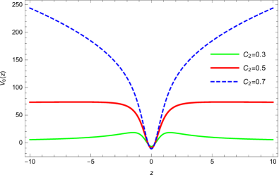
(a) $V_{0}(z)$

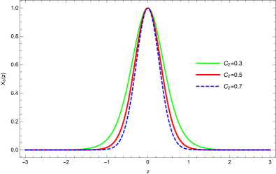
(b) $\chi_{0}\left(z\right)$

Figure 1: The effective potentials $\displaystyle V_{0}\left(z\right)$ in (a), and the shapes of scalar zero-mode $\displaystyle\chi_{0}\left(z\right)$ in (b). The parameters are set as $\displaystyle C_{1}=10,k=1$ and $\displaystyle C_{2}=0.3,0.5,0.7$.

Analysis of the mass spectra for the scalar KK modes (in Fig. 2) reveals that the ground state corresponds to the zero mode (a bound state), and all the massive KK modes are bound modes. Notably, the number of bound modes increases with both the parameters $C_{1}$ and $C_{2}$.

(a) $C_{1}=15,k=1,C_{2}=0.5$

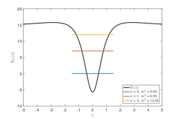
(b) $C_{1}=10,k=1,C_{2}=0.5$

(c) $C_{1}=10,k=1,C_{2}=0.6$

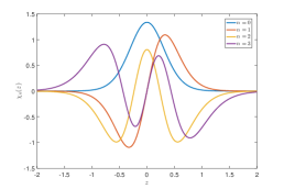
(d) $C_{1}=15,k=1,C_{2}=0.5$

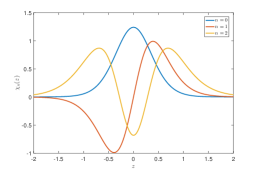
(e) $C_{1}=10,k=1,C_{2}=0.5$

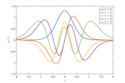
(f) $C_{1}=10,k=1,C_{2}=0.6$

Figure 2: The upper row shows the potential $\displaystyle V_{0}\left(z\right)$ with the black line representing the potential and the colored lines indicating the position of mass spectra. The lower row presents the corresponding solutions of $\displaystyle\chi_{0}\left(z\right)$. Parameters are varied as $\displaystyle C_{1}=15,10,10;k=1$ and $\displaystyle C_{2}=0.5,0.5,0.6$, respectively.

$Case$ II: Coupling with the scalar field, $\displaystyle F\left(R,\varphi\right)=\lambda\left(\varphi_{0}^{2}-\varphi^{2}\right)^{t}$. By substituting equations (31) and (32) into the expressions for the potential function (39) and the zero-mode function (43), we obtain the zero-mode function:

$$\chi_{\varphi}\left(z\right)=\frac{\sqrt{\left(\frac{1}{1+k^{2}z^{2}}\right)^{t}}}{(1+k^{2}z^{2})^{\frac{3}{4}}},$$ (51)

and the potential function:

$$V_{\varphi}\left(z\right)=\frac{k^{2}(3+2t)(-2+k^{2}(5+2t)z^{2})}{4(1+k^{2}z^{2})^{2}}.$$ (52)

It is evident that:

$$\chi_{\varphi}\left(z\rightarrow\infty\right)\approx\frac{1}{z^{\frac{3}{2}+t}},\quad V_{\varphi}\left(z\rightarrow\infty\right)=0.$$ (53)

Here, $t$ is a positive constant. Thus, the zero-mode function of scalar fields is convergent and localizable solely under scalar field coupling. By selecting different values of $t$, various potential functions and zero-mode cases can be obtained, as depicted in Fig. 3.

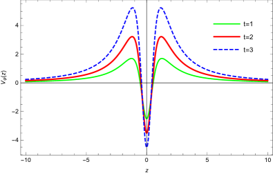
(a) $V_{\varphi}(z)$

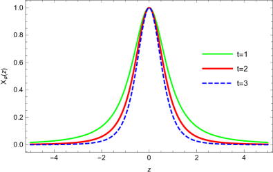
(b) $\chi_{\varphi}(z)$

Figure 3: The effective potentials $V_{\varphi}(z)$ in (a), and the shapes of scalar zero-mode $\chi_{\varphi}(z)$ in (b). Parameters are set as $\lambda=10,k=1$ and $t=1,2,3$.

In conclusion, the analysis of the coupling to both the gravitational field and scalar field has been carried out separately. It has been observed that the parameter $C_{2}$ influences the convergence of the zero-mode when coupled to the gravitational field, leading to variations in the behavior of the effective potential function at infinity. On the other hand, the parameters $C_{1}$ and $k$ impact the depth of the potential well when the potential function approaches a finite value (with $C_{2}=\frac{1}{2}$), where larger values result in deeper potential wells and an increase in the number of bound states. When coupled to a scalar field, the parameter $t$ does not affect the convergence of the zero-mode case but alters the height of the potential function, with larger values of $t$ leading to a higher potential peak.

IV.2 $\displaystyle U(1)$ gauge vector field

In general, $\displaystyle A_{\mu}$ denotes the $\displaystyle U(1)$ gauge vector fields with $\displaystyle q=1$. This field is utilized to describe particles with spin-1. Given that there are canonical degrees of freedom, we initially choose the canonical gauge $\displaystyle A_{z}=0$ and subsequently perform the KK decomposition.

Considering the coupling function and the background spacetime, the action of the five-dimensional vector field is expressed as:

$$S_{\text{vector}}=-\frac{1}{4}\int d^{5}x\sqrt{-g}F(R,\varphi)F_{MN}F^{MN},$$ (54)

where $\displaystyle F_{MN}=\partial_{M}A_{N}-\partial_{N}A_{M}$. Based on the flat metric (14), the equations of motion can be decomposed into the following form:

$$\partial_{\mu}\left(\sqrt{-g}F(R,\varphi)F^{\mu\nu}\right)+\partial_{z}\left(\sqrt{-g}F(R,\varphi)F^{z\nu}\right) =0,$$ (55)

$$\partial_{\mu}\left(\sqrt{-g}F(R,\varphi)F^{\mu z}\right) =0.$$

By adopting the KK decomposition

$$A_{\mu}(x^{\mu},z)=\sum_{n}a_{\mu}^{(n)}(x^{\mu})\rho_{n}(z)e^{-\frac{1}{2}A}F(R,\varphi)^{-\frac{1}{2}},$$ (56)

we obtain the specific form of the Schrödinger-like equation for the vector field:

$$\left[-\partial_{z}^{2}+V_{1}(z)\right]\rho_{n}(z)=m_{n}^{2}\rho_{n}(z),$$ (57)

where the potential of the vector field is given by:

$$V_{1}(z) = \frac{1}{4}A^{\prime 2}(z)+\frac{1}{2}A^{\prime\prime}(z)+\frac{F^{\prime\prime}(R,\varphi)}{2F(R,\varphi)}$$ (58)

$$+\frac{F^{\prime}(R,\varphi)A^{\prime}(z)}{2F(R,\varphi)}-\frac{F^{\prime 2}(R,\varphi)}{4F^{2}(R,\varphi)},$$

and $\displaystyle m_{n}$ represent the masses of the vector KK modes.

Similar to the case of scalar fields, orthogonal normalization is achieved with

$$\int\rho_{m}(z)\rho_{n}(z)dz=\delta_{mn}.$$ (59)

The 4D effective action of the vector field can be derived as:

$$S_{\text{vector}}=-\frac{1}{4}\sum_{n}\int d^{4}x\sqrt{-g}\left(f_{\mu\nu}f^{\mu\nu}+m_{n}^{2}a_{\mu}a^{\mu}\right),$$ (60)

where $\displaystyle f_{\mu\nu}f^{\mu\nu}=\partial_{\mu}a_{\nu}-\partial_{\nu}a_{\mu}$ is the 4D field strength.

By setting $\displaystyle m_{n}=0$, we obtain the specific form of the zero-mode vector field as:

$$\rho_{0}(z)=N_{1}e^{\frac{1}{2}A(z)}F(R,\varphi)^{\frac{1}{2}},$$ (61)

where $N_{1}$ is the normalization constant for the $U(1)$ gauge vector field.

$Case$ I: Coupling with gravity, $\displaystyle F\left(R,\varphi\right)=G\left(R\right)$. By substituting Eqs. (31) and (32) into the expressions for the potential function (58) and the zero-mode (61), we obtain the $\displaystyle U(1)$ vector gauge field zero-mode as:

$$\rho_{0}\left(z\right)=\frac{\sqrt{e^{C_{1}-(\frac{5}{7})^{C_{2}}\!\>C_{1}\!\>(\frac{1}{1+k^{2}\!\>z^{2}})^{-C_{2}}}}}{\sqrt{e^{C_{1}-(\frac{5}{7})^{C_{2}}C_{1}}}(1+k^{2}\!\>z^{2})^{\frac{1}{4}}}.$$ (62)

To find the second order derivative of $\displaystyle{\rho}_{0}\left(z\right)$ and its value at $\displaystyle z=0$, we have:

$$\rho^{\prime\prime}_{z}\left(z=0\right)=\beta\sqrt{\text{e}^{C_{1}\left(1-\left(\frac{5}{7}\right)^{C_{2}}\right)}}k^{2},$$ (63)

where $\displaystyle\beta=-\frac{1}{2}\times 7^{C_{2}}\left(7^{C_{2}}+2\times 5^{C_{2}}C_{1}C_{2}\right)$. Therefore, it can be concluded that the second-order derivative $\displaystyle\rho_{z}^{{}^{\prime\prime}}\left(z\right)<0$ at $z=0$, indicating that the zero-mode is a convex function.

The potential function is given by:

$$V_{1}\left(z\right) = \frac{1}{4}\!\>k^{2}\!\>\bigg{(}\frac{1}{1+k^{2}\!\>z^{2}}\bigg{)}^{2-2\!\>C_{2}}\!\>\bigg{(}4\!\>(\frac{25}{49})^{C_{2}}\!\>{C_{1}}^{2}\!\>{C_{2}}^{2}\!\>k^{2}\!\>z^{2}$$ (64)

$$+(\frac{1}{1+k^{2}\!\>z^{2}})^{2\!\>C_{2}}\!\>(-2+3\!\>k^{2}\!\>z^{2})-4\times\!\>5^{C_{2}}C_{1}C_{2}$$

$$\times\!\>(\frac{1}{7+7\!\>k^{2}\!\>z^{2}})^{C_{2}}\!\>(1+2\!\>(-1+C_{2})\!\>k^{2}\!\>z^{2})\bigg{)}.$$

The limit of $\displaystyle V_{1}\left(z\right)$ as $z$ approaches infinity is:

$$\underset{z\rightarrow+\infty}{\lim}V_{1}\left(z\right)=0.$$ (65)

For a boundary analysis of the specific behavior of the potential function at infinity, we approximate:

$$V_{1}\left(z\rightarrow\infty\right)\approx A_{1}(\frac{1}{z})^{2-2\!\>C_{2}},$$ (66)

where $\displaystyle A_{1}=-2\times\!\>5^{C_{2}}\!\>C_{1}\!\>(-1+C_{2})\!\>C_{2}\!\>k$.

From the above, we can derive the conditions for the value of $\displaystyle V_{1}\left(z\right)$ on the boundary, which can be verified by the limit of $\displaystyle V_{2}\left(z\right)$, namely,

$$V_{1}\left(z\rightarrow\pm\infty\right)=\begin{cases}+\infty,&C_{2}>\small{\frac{1}{2}}\\ V_{const},&C_{2}=\frac{1}{2}\\ 0,&0<C_{2}<\frac{1}{2},\\ \end{cases}$$ (67)

where $\displaystyle V_{const}=\frac{5}{28}C_{1}^{2}k^{2}$. Clearly, $V_{const}>0$, and its value depends on the parameters $C_{1}$ and $k$. The larger the values of $C_{1}$ and $k$, the larger the value of $V_{const}$, the deeper the potential well, and the greater the number of bound states that can be obtained.

Finally, we perform a convergence analysis of the wave function for the zero-mode case:

$${\rho}_{0}\left(z\rightarrow\infty\right)\approx\sqrt{C\text{e}^{-z^{-2\!\>C_{2}}}},$$ (68)

where $\displaystyle C=\text{e}^{C_{1}-(\frac{5}{7})^{C_{2}}}$, and $C_{2}>0$. From the above, we derive that the wave function converges when $\displaystyle C_{2}>0$.

To more intuitively reflect the content of the above analysis, we have plotted the results of numerical calculations, with detailed information presented in Fig. 4. The figure demonstrates that the behaviors of the effective potential align well with the conclusions (67). Subsequently, we will explicitly outline the localization of the massive KK modes in the cases of parameters $C_{1}$ and $C_{2}$.

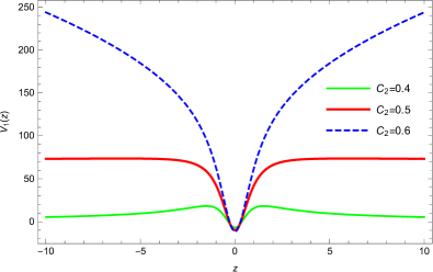
(a) $V_{1}\left(z\right)$

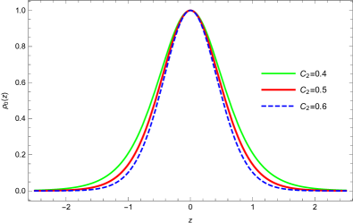
(b) $\rho_{0}\left(z\right)$

Figure 4: The effective potentials $\displaystyle V_{1}\left(z\right)$ in (a), and the shapes of the scalar zero-mode $\displaystyle\rho_{0}\left(z\right)$ in (b). The parameters are set as $\displaystyle C_{1}=20,k=1$ and $\displaystyle C_{2}=0.4,0.5,0.6$.

Additionally, we have computed several other bound states whose wave functions are labeled and plotted on the potential function in Fig. 5.

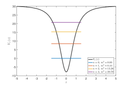
(a) $C_{1}=15,k=1,C_{2}=0.5$

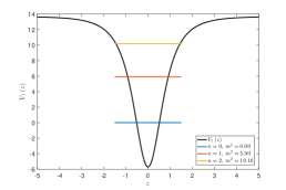
(b) $C_{1}=10,k=1,C_{2}=0.5$

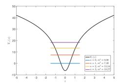
(c) $C_{1}=10,k=1,C_{2}=0.6$

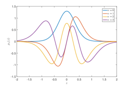
(d) $C_{1}=10,k=1,C_{2}=0.5$

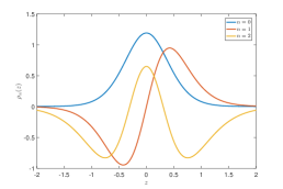
(e) $C_{1}=10,k=1,C_{2}=0.5$

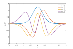
(f) $C_{1}=10,k=1,C_{2}=0.6$

Figure 5: The upper row shows the potential $\displaystyle V_{1}\left(z\right)$ with the black line representing the potential and the colored lines indicating the position of mass spectra. The lower row presents the corresponding solutions of $\displaystyle\rho_{0}\left(z\right)$. Parameters are varied as $\displaystyle C_{1}=15,10,10;k=1$ and $\displaystyle C_{2}=0.5,0.5,0.6$, respectively.

$Case$ II: Coupling with the scalar field, $\displaystyle F\left(R,\varphi\right)=\lambda\left(\varphi_{0}^{2}-\varphi^{2}\right)^{t}$. Substituting Equations (31) and (32) into the expressions for the potential function (58) and the zero-mode (61) yields the zero-mode function:

$$\rho_{\varphi}\left(z\right)=\frac{\sqrt{(\frac{147}{29})^{t}\lambda\left(\frac{1}{1+k^{2}z^{2}}\right)^{t}}}{(1+k^{2}z^{2})^{\frac{1}{4}}},$$ (69)

and the potential function:

$$V_{\varphi}\left(z\right)=\frac{k^{2}(1+2t)(-2+k^{2}(3+2t)z^{2})}{4(1+k^{2}z^{2})^{2}}.$$ (70)

It is evident that:

$$\rho_{\varphi}\left(z\rightarrow\infty\right)\approx\frac{C}{z^{\frac{1}{2}+t}},\quad V_{\varphi}\left(z\rightarrow\infty\right)=0.$$ (71)

When $\displaystyle t>\frac{1}{2}$, the zero-mode function of vector fields is convergent and localizable with scalar field coupling only. By selecting different values of $t$, various potential functions and zero-mode configurations can be obtained, as depicted in Fig. 6. In addition, it can be seen from Fig. 6 that different values of the parameter $t$ lead to changes in the potential function potential barriers. Specifically: in the case of zero-mode convergence, the larger the value of $t$, the higher the potential barrier. The parameter $k$ will have the same effect, but will not affect the convergence of the zero mode.

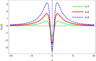
(a) $V_{\varphi}\left(z\right)$

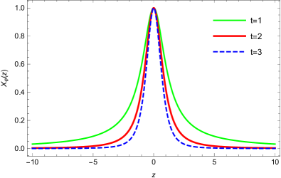
(b) $\chi_{\varphi}\left(z\right)$

Figure 6: The effective potentials $\displaystyle V_{\varphi}\left(z\right)$ in (a), and the shapes of the scalar zero-mode $\displaystyle\chi_{\varphi}\left(z\right)$ in (b). The parameters are set as $\displaystyle\lambda=10,k=1$ and $\displaystyle t=1,2,3$.

In summary, the analysis of coupling to both gravitational and scalar fields reveals distinct influences on the convergence of the zero mode and the behavior of the effective potential function at infinity. Specifically, the parameter $C_{2}$ significantly impacts the convergence of the zero mode when coupled to the gravitational field, resulting in varied behaviors of the effective potential at infinity. The parameters $C_{1}$ and $k$ influence the depth of the potential well when the potential function approaches a finite value ($C_{2}=\frac{1}{2}$), where larger values lead to deeper potential wells and an increase in the number of bound states. Conversely, when coupled to a scalar field, the parameter $t$ affects the convergence of the zero-mode case, ensuring the convergence of the vector zero mode for $t>\frac{1}{2}$. Additionally, the parameter $\lambda$ influences the zero-mode function.

IV.3 Kalb-Ramond field

In the case where $\displaystyle q=2$, the $q$-form field manifests as a KR field. This second-order antisymmetric tensor field, initially introduced in string theory, emerges as a massless mode. In a four-dimensional spacetime, the KR field is dual to a scalar field. Conversely, within higher-dimensional spacetimes, it signifies the presence of new particles. Therefore, the study of field localization in braneworld scenarios becomes imperative.

Considering a specific coupling function, the action for the free KR field in a five-dimensional spacetime is given by:

$$S_{\text{KR}}=-\int{d^{5}x\sqrt{-g}F\left(R,\varphi\right)H_{MNL}H^{MNL}},$$ (72)

where $\displaystyle H_{MNL}=\partial_{[M}B_{NL]}$ denotes the field strength of the KR field. Employing a metric of the prescribed form (14), the equations of motion decompose into:

$$\partial_{\mu}\left(\sqrt{-g}F\left(R,\varphi\right)H^{\mu\nu\gamma}\right)+\partial_{z}\left(\sqrt{-g}F\left(R,\varphi\right)H^{z\nu\gamma}\right)=0,$$ (73)

$$\partial_{\mu}\left(\sqrt{-g}F\left(R,\varphi\right)H^{\mu\nu z}\right)=0.$$

By selecting the gauge $\displaystyle B_{\mu 5}=0$ and utilizing the KK decomposition:

$$B_{\mu\nu}\left(x^{\mu},z\right)=\sum_{n}{\hat{b}_{\mu\nu}^{\left(n\right)}\left(x^{\mu}\right)u^{\left(n\right)}\left(z\right)}\text{e}^{\frac{1}{2}A}F\left(R,\varphi\right)^{-\frac{1}{2}},$$ (74)

we derive a Schrödinger-like equation for the KR field:

$$\left[-\partial_{z}^{2}+V_{2}\left(z\right)\right]{u}^{\left(n\right)}\left(z\right)=m_{n}^{2}{u}^{\left(n\right)}\left(z\right),$$ (75)

where the potential is expressed as:

$$V_{2}\left(z\right) = \frac{1}{4}A^{\prime 2}\left(z\right)-\frac{1}{2}A^{\prime\prime}\left(z\right)+\frac{F^{\prime\prime}\left(R,\varphi\right)}{2F\left(R,\varphi\right)}$$ (76)

$$-\frac{F^{\prime}\left(R,\varphi\right)}{2F\left(R,\varphi\right)}A^{\prime}\left(z\right)-\frac{F^{\prime 2}\left(R,\varphi\right)}{4F^{2}\left(R,\varphi\right)}.$$

Assuming orthogonal normalization:

$$\int{u_{m}\left(z\right)u_{n}\left(z\right)dz=\delta_{mn}},$$ (77)

the four-dimensional effective action, approximated from the five-dimensional one, is:

$$S_{\text{KR}}=\sum_{n}{\int{d^{4}x\sqrt{-g}(\hat{h}_{\mu\nu\gamma}^{\left(n\right)}\hat{h}^{\left(n\right)\mu\nu\gamma}+\frac{1}{3}m_{n}^{2}\hat{b}_{\mu\nu\gamma}^{\left(n\right)}\hat{b}^{\left(n\right)\mu\nu\gamma})}}.$$ (78)

For $\displaystyle m_{n}^{2}=0$, the zero-mode form of the KR field can be resolved from equation (75):

$$u_{0}\left({z}\right)=N_{2}\text{e}^{-\frac{1}{2}\!\>A\left(z\right)}\!\>F\left(R,\varphi\right)^{\frac{1}{2}}$$ (79)

with $N_{2}$ the normalization constant.

$Case$ I: Coupling with gravity, $\displaystyle F(R,\varphi)=G(R)$. By substituting Eqs. (31) and (32) into the potential function expression (76) and the zero-mode expression (79), the zero-mode of the KR field is obtained as:

$$u_{0}\left(z\right)=\frac{\sqrt{\text{e}^{C_{1}-(\frac{5}{7})^{C_{2}}\!\>C_{1}(\frac{1}{1+k^{2}\!\>z^{2}})^{-C_{2}}}}\!\>(1+k^{2}\!\>z^{2})^{\frac{1}{4}}}{\sqrt{\text{e}^{C_{1}-(\frac{5}{7})^{C_{2}}C_{1}}}}.$$ (80)

To find the second-order derivative of $u_{0}\left(z\right)$ and evaluate it at $z=0$, we derive:

$$u^{\prime\prime}_{z}\left(z=0\right)=\sigma\sqrt{\text{e}^{C_{1}\left(1-\left(\frac{5}{7}\right)^{C_{2}}\right)}}k^{2},$$ (81)

where $\sigma=-\left(\frac{5}{7}\right)^{C_{2}}C_{1}C_{2}$. Thus, it can be inferred that the second-order derivative $u_{z}^{{}^{\prime\prime}}\left(z\right)<0$ at $z=0$, indicating the zero-mode is a convex function.

In addition, the potential function (76) is given by:

$$V_{2}\left(z\right) = \frac{1}{4}k^{2}\bigg{(}\frac{1}{1+k^{2}z^{2}}\bigg{)}^{2-2C_{2}}\bigg{(}4(\frac{25}{49})^{C_{2}}{C_{1}}^{2}{C_{2}}^{2}k^{2}z^{2}$$ (82)

$$+(\frac{1}{1+k^{2}z^{2}})^{2C_{2}}(-2+3k^{2}z^{2})-4\times 5^{C_{2}}C_{1}C_{2}$$

$$\times(\frac{1}{7+7k^{2}z^{2}})^{C_{2}}(1+2C_{2}k^{2}z^{2})\bigg{)}.$$

The limit of $V_{2}\left(z\right)$ as $z$ approaches infinity is:

$$\lim_{z\rightarrow+\infty}V_{2}\left(z\right)=0.$$ (83)

For a boundary analysis of the specific behavior of potential function at infinity, we approximate:

$$V_{2}\left(z\rightarrow\infty\right)\approx B_{2}(\frac{1}{z})^{2-2C_{2}},$$ (84)

where $B_{2}=-2\times 5^{C_{2}}C_{1}{C_{2}}^{2}k^{4}$.

From the above, we can derive the conditions for the value of $V_{2}\left(z\right)$ on the boundary, which can be verified by the limit of $V_{3}\left(z\right)$, namely,

$$V_{2}\left(z\rightarrow\pm\infty\right)=\begin{cases}+\infty,&C_{2}>\frac{1}{2}\\ V_{const},&C_{2}=\frac{1}{2}\\ 0,&0<C_{2}<\frac{1}{2},\end{cases}$$ (85)

where $V_{const}=\frac{5}{28}C_{1}^{2}k^{2}$. Clearly, $V_{const}>0$, and its value is dependent on the parameters $C_{1}$ and $k$. The larger the values of $C_{1}$ and $k$ are, the larger $V_{const}$ is, the deeper the potential well becomes, and the more bound states can be obtained.

Finally, we perform a convergence analysis of the wave function for the zero-mode case:

$$u_{0}\left(z\rightarrow\infty\right)\approx\sqrt{C\text{e}^{-z^{-2C_{2}}}},$$ (86)

where $C=\text{e}^{C_{1}-(\frac{5}{7})^{C_{2}}}$, and $C_{2}>0$. From the above, we can derive that the zero-mode case is convergent when $C_{2}>0$.

To more intuitively reflect the content of the above analysis, numerical calculations have been performed, and the detailed information is depicted in Fig. 7. The figure demonstrates that the behaviors of the effective potential align well with the conclusions (85). Additionally, a number of other bound states have been computed, with their wave functions plotted against the potential function in Fig. 8.

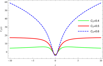
(a) $V_{2}\left(z\right)$

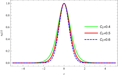
(b) $u_{0}\left(z\right)$

Figure 7: The effective potentials $\displaystyle V_{2}\left(z\right)$ in (a), and the shapes of scalar zero-mode $\displaystyle u_{0}\left(z\right)$ in (b). The parameters are set as $\displaystyle C_{1}=20,k=1$ and $\displaystyle C_{2}=0.4,0.5,0.6$.

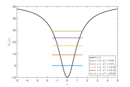
(a) $C_{1}=20,k=1,C_{2}=0.5$

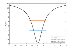
(b) $C_{1}=10,k=1,C_{2}=0.5$

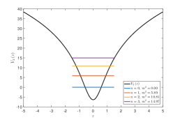
(c) $C_{1}=10,k=1,C_{2}=0.6$

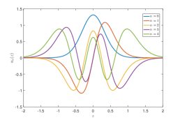
(d) $C_{1}=20,k=1,C_{2}=0.5$

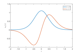
(e) $C_{1}=10,k=1,C_{2}=0.5$

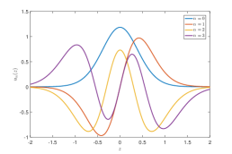
(f) $C_{1}=10,k=1,C_{2}=0.6$

Figure 8: The upper row shows the potential $\displaystyle V_{2}\left(z\right)$ with the black line representing the potential and the colored lines indicating the position of mass spectra. The lower row presents the corresponding solutions of $\displaystyle u_{0}\left(z\right)$. Parameters are varied as $\displaystyle C_{1}=20,10,10;k=1$ and $\displaystyle C_{2}=0.5,0.5,0.6$, respectively.

$Case$ II: Coupling with the scalar field, $\displaystyle F\left(R,\varphi\right)=\lambda\left(\varphi_{0}^{2}-\varphi^{2}\right)^{t}$. Substituting equations (31) and (32) into the expressions for the potential function (76) and the zero-mode (79), we obtain the zero-mode function as:

$$u_{\varphi}(z)=\sqrt{\left(\frac{147}{29}\right)^{t}\lambda\left(\frac{1}{1+k^{2}z^{2}}\right)^{t}}(1+k^{2}z^{2})^{\frac{1}{4}},$$ (87)

and the potential function as:

$$V_{\varphi}(z)=\frac{k^{2}(2-4t-k^{2}z^{2}+4k^{2}t^{2}z^{2})}{4(1+k^{2}z^{2})^{2}}.$$ (88)

It is evident that we can deduce:

$$u_{\varphi}(z\rightarrow\infty)=Cz^{\frac{1}{2}-t},\quad V_{\varphi}(z\rightarrow\infty)=0.$$ (89)

When $t>{3}/{2}$, the zero-mode function under tensor fields is convergent and localizable with scalar field coupling. By selecting different values of $t$, various potential functions and zero-mode configurations can be obtained, as depicted in Fig. 9. Additionally, it can be observed from Fig. 9 that different values of the parameter $t$ lead to changes in the potential barriers. Specifically, in the case of zero-mode convergence, the higher the value of $t$, the higher the potential barrier. The parameter $k$ will have a similar effect but does not influence the convergence of the zero mode.

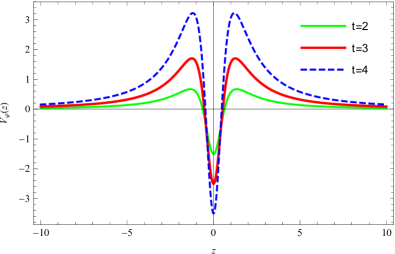
(a) $V_{\varphi}(z)$

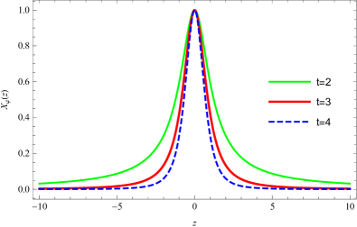
(b) $\chi_{\varphi}(z)$

Figure 9: The effective potentials $V_{\varphi}(z)$ in (a), and the shapes of the scalar zero-mode $\chi_{\varphi}(z)$ in (b). The parameters are set as $\lambda=10,k=1$ and $t=2,3,4$.

In summary, the analysis of coupling to both gravitational and scalar fields reveals distinct influences on the convergence of the zero mode and the behavior of the effective potential function at infinity. Specifically, the parameter $C_{2}$ significantly impacts the convergence of the zero mode when coupled to the gravitational field, resulting in varied behaviors of the effective potential at infinity. The parameters $C_{1}$ and $k$ influence the depth of the potential well when the potential function approaches a finite value ($C_{2}=\frac{1}{2}$), where larger values lead to deeper potential wells and an increase in the number of bound states. Conversely, when coupled to a scalar field, the parameter $t$ affects the convergence of the zero-mode case, ensuring the convergence of the zero mode of KR field for $t>\frac{3}{2}$. Additionally, the parameter $\lambda$ influences the zero-mode function. In the case of zero-mode convergence, the larger the value of $t$, the higher the potential barrier. The parameter $k$ will have a similar effect but will not affect the convergence of the zero mode.

V Conclusions

In this paper, we embark on a comprehensive examination of the localization phenomena on the domain wall brane within the context of squared curvature gravity in a five-dimensional spacetime framework. The initial segment of our study is dedicated to reviewing the mechanisms through which the tensor field achieves localization when coupled with the gravitational field in this brane model. Building upon this foundational understanding, we extend our exploration to the localization dynamics of the $q$-form field on the brane, taking into account its coupling interactions. The coupling function under consideration is bifurcated into two distinct segments: one associated with the gravitational field and the other with the background scalar field. Through meticulous calculations, we derive the zero-mode function, formulate the Schrödinger-like equation, and quantify the four-dimensional effective action for the $q$-form field localization on the brane. Furthermore, we delve into a detailed analysis of the localization properties of 0-form, 1-form, and 2-form fields when coupled to both the gravitational field and the scalar field on specific membranes. Our investigation is enriched by numerical calculations, from which we extract a diverse array of results depicted through relevant figures.

Our findings illuminate the critical role of the parameter $\displaystyle C_{2}$ in the localization process of $q$-form fields to the gravitational field alone within a five-dimensional spacetime. The behavior of the wave function, as described by the Schrödinger-like equation at infinity, diverges into three distinct scenarios contingent upon the values of $\displaystyle C_{2}$:

• For $\displaystyle C_{2}<\frac{1}{2}$, the mass spectrum capable of localization is confined to the zero mode, with no additional mass spectra observable.

• A value of $\displaystyle C_{2}=\frac{1}{2}$ yields a finite number of localizable mass spectra.

• When $\displaystyle C_{2}>\frac{1}{2}$, an infinite array of localizable mass spectra emerges.

This delineation necessitates a discussion on the conditions where $\displaystyle C_{2}$ surpasses zero, a prerequisite for the existence of localized zero modes.

Moreover, the parameter $\displaystyle t$ emerges as a pivotal factor in the context of $q$-form field coupling to a scalar field exclusively. For 0-form fields, the presence of $\displaystyle t$ does not influence the zero mode. Conversely, the existence of a localized zero mode for 1-form fields requires $\displaystyle t>{1}/{2}$, while for 2-form fields, this threshold is raised to $\displaystyle t>{3}/{2}$.

In conclusion, our work not only addresses and fills the gaps left by previous studies that overlooked scalar field coupling but also advances the analytical framework for examining the localization of $q$-form fields on domain wall branes in the presence of gravitational and scalar field couplings. By shedding light on these complex interactions, we pave the way for future investigations into the diverse mechanisms of localization across different coupling forms, thereby enriching the theoretical landscape of higher-dimensional physics and its implications for the fabric of our universe.

VI acknowledgments

This work was supported by the National Natural Science Foundation of China (Grants No. 11305119, No. 11705070, and No. 11405121), the Natural Science Basic Research Plan in Shaanxi Province of China (Program No. 2020JM-198), the Fundamental Research Funds for the Central Universities (Grants No. JB170502), and the 111 Project (B17035).

References

- (1) Th. Kaluza, On the Problem of Unity in Physics, Sitzungsber. Preuss. Akad. Wiss. Berlin. (Math. Phys.) 1921 (1921) 966-972.
- (2) O. Klein, Quantum Theory and Five-Dimensional Theory of Relativity, Z. Phys. 37 (1926) 895-906.
- (3) I. Antoniadis, N. Arkani-Hamed, S. Dimopoulos, G. Dvali, New dimensions at a millimeter to a fermi and superstrings at a TEV, JHEP 9807 (1998) 001.
- (4) L. Randall and R. Sundrum, A Large Mass Hierarchy from a Small Extra Dimension, Phys. Rev. Lett. 83 (1999) 3370, [arXiv:hep-ph/9905221].
- (5) L. Randall and R. Sundrum, An Alternative to Compactification, Phys. Rev. Lett. 83 (1999) 4690, [arXiv:hep-th/9906064].
- (6) O. DeWolfe, D. Z. Freedman, S. S. Gubser, et al., Modeling the fifth dimension with scalars and gravity, Phys. Rev. D 62 (2000) 046008.
- (7) C. Csaki, J. Erlich, T. J. Hollowood, et al., ‘Universal aspects of gravity localized on thick branes, Nucl. Phys. B 581 (2000) 309-338.
- (8) M. Gremm, Four-dimensional gravity on a thick domain wall, Phys. Lett. B 478 (2000) 434-438.
- (9) H. Guo, L. L. Wang, C. E. Fu, et al., Gravity and matter on a pure geometric thick polynomial f(R) brane, Phys. Rev. D 107 (2023) 104017.
- (10) Y. Grossman and M. Neubert, Neutrino masses and mixings in non-factorizable geometry, Phys. Lett. B 474 (2000) 361-371.
- (11) B. Bajc and G. Gabadadze, Localization of matter and cosmological constant on a brane in anti de Sitter space, Phys. Lett. B 474 (2000) 282-291.
- (12) S. Randjbar-Daemi and M. Shaposhnikov, Fermion zero-modes on brane-worlds, Phys. Lett. B 492 (2000) 361-364.
- (13) I. Oda, Localization of matters on a string-like defect, Phys. Lett. B 496 (2000) 113-121.
- (14) A. Kehagias and K. Tamvakis, Localized gravitons, gauge bosons and chiral fermions in smooth spaces generated by a bounce, Phys. Lett. B 504 (2001) 38-46.
- (15) I. Oda, Localization of bulk fields on AdS4 brane in AdS5, Phys. Lett. B 508 (2001) 96-102.
- (16) S. Ichinose, Fermions in Kaluza-Klein and Randall-Sundrum theories, Phys. Rev. D 66 (2002) 104015.
- (17) R. Davies, D. P. George, and R. R. Volkas, Standard model on a domain-wall brane?, Phys. Rev. D 77 (2008) 124038.
- (18) Y. X. Liu, L. D. Zhang, S. W. Wei, et al., Localization and mass spectrum of matters on Weyl thick branes, JHEP 08 (2008) 041.
- (19) Y. X. Liu, J. Yang, Z. H. Zhao, et al., Fermion localization and resonances on a de Sitter thick brane, Phys. Rev. D 80 (2009) 065019.
- (20) Y. X. Liu, C. E. Fu, L. Zhao, et al., Localization and mass spectra of fermions on symmetric and asymmetric thick branes, Phys. Rev. D 80 (2009) 065020.
- (21) Y. X. Liu, H. Guo, C. E. Fu, et al., Localization of matters on Anti-de Sitter thick branes, JHEP 02 (2010) 1-24.
- (22) Y. X. Liu, H. Guo, C. E. Fu, et al., Localization of gravity and bulk matters on a thick anti-de Sitter brane, Phys. Rev. D 84 (2011) 044033.
- (23) P. R. Archer and S. J. Huber, Reducing constraints in a higher dimensional extension of the Randall and Sundrum model, JHEP 03 (2011) 1-28.
- (24) C. E. Fu, Y. X. Liu, K. Yang, et al., q-Form fields on p-branes JHEP 10 (2012) 1-14.
- (25) H. Guo, A. Herrera-Aguilar, Y. X. Liu, et al., Localization of bulk matter fields, the hierarchy problem and corrections to Coulomb’s law on a pure de Sitter thick braneworld, Phys. Rev. D 87 (2013) 095011.
- (26) P. Jones, G. Munoz, and D. Singleton, Field localization and the Nambu-Jona-Lasinio mass generation mechanism in an alternative five-dimensional brane model, Phys. Rev. D 88 (2013) 025048.
- (27) Q. Y. Xie, J. Yang, and L. Zhao, Resonance mass spectra of gravity and fermion on Bloch branes, Phys. Rev. D 88 (2013) 105014.
- (28) F. W. V. Costa, J. E. G. Silva, and C. A. S. Almeida, Gauge vector field localization on a 3-brane placed in a warped transverse resolved conifold, Phys. Rev. D 87 (2013) 125010.
- (29) Z. H. Zhao, Y. X. Liu, and Y. Zhong, U(1) gauge field localization on a Bloch brane with Chumbes-Holf da Silva-Hott mechanism, Phys. Rev. D 90 (2014) 045031.
- (30) G. Alencar, R. R. Landim, M. O. Tahim, et al., Gauge field localization on the brane through geometrical coupling, Phys. Lett. B 739 (2014) 125-127.
- (31) Y. T. Lu, H. Guo, and C. E. Fu, Localization of -form field on the brane-world by coupling with gravity, arXiv preprint arXiv:2401.11688, 2024.
- (32) G. Alencar, I. C. Jardim, R. R. Landim, et al., Generalized nonminimal couplings in Randall-Sundrum scenarios, Phys. Rev. D 93 (2016) 124064.
- (33) Z. H. Zhao, Q. Y. Xie, C. E. Fu, et al., Localization of U(1) gauge field by non-minimal coupling with gravity in braneworlds, JCAP 2023 (2023) 010.
- (34) Y. X. Liu, Y. Zhong, Z. H. Zhao, et al., Domain wall brane in squared curvature gravity, JHEP 2011 (2011) 1-18, [arXiv:1104.3188].
- (35) C. E. Fu, Y. Zhong, Q. Y. Xie, et al., Localization and mass spectrum of -form fields on branes, Phys. Lett. B 757 (2016) 180-186.
- (36) C. E. Fu, Y. X. Liu, H. Guo, et al., New localization mechanism and Hodge duality for -form field, Phys. Rev. D 93 (2016) 064007.
- (37) H. Guo, Y. T. Lu, C. L. Wang, et al., Localization of scalar field on the brane-world by coupling with gravity, arXiv preprint arXiv:2310.01451 (2023).
- (38) Y. X. Liu, Introduction to extra dimensions and thick braneworlds, in Memorial volume for Yi-shi Duan, (2018) 211-275.
- (39) C.-E. Fu, Y.-X. Liu, K. Yang, and S.-W. Wei, -Form fields on -branes, JHEP 2012 (2012) 060.
- (40) D. Bazeia, F. A. Brito, and J. R. Nascimento, Supergravity brane worlds and tachyon potentials, Phys. Rev. D 68 (2003) 085007.
- (41) A. Herrera-Aguilar, A. D. Rojas, and E. Santos, Localization of gauge fields in a tachyonic de Sitter thick braneworld, Eur. Phys. J. C 74 (2014) 1-6.
- (42) Z. H. Zhao and Q. Y. Xie, Localization of U(1) gauge vector field on flat branes with five-dimension (asymptotic) AdS5 spacetime,JHEP 2018 (2018) 1-13, [arXiv:1712.09843].
- (43) T. Appelquist, A. Chodos, and P. G. O. Freund, Modern Kaluza-Klein Theories, Addison-Wesley (1987).
- (44) N. Arkani-Hamed, S. Dimopoulos, and G. Dvali, The hierarchy problem and new dimensions at a millimeter, Phys. Lett. B 429 (1998) 263-272.
- (45) E. Witten, Anti de Sitter space and holography, arXiv preprint hep-th/9802150 (1998).
- (46) S. S. Gubser, I. R. Klebanov, and A. M. Polyakov, ‘Gauge theory correlators from non-critical string theory, Phys. Lett. B 428 (1998) 105-114.
- (47) J. Maldacena, The large-N limit of superconformal field theories and supergravity, Int. J. Theor. Phys. 38 (1999) 1113-1133.
- (48) M. O. Tahim, W. T. Cruz, and C. A. S. Almeida, Tensor gauge field localization in branes, Phys. Rev. D 79 (2009) 085022.
- (49) W. T. Cruz, M. O. Tahim, and C. A. S. Almeida, Results in Kalb-Ramond field localization and resonances on deformed branes, Europhys. Lett. 88 (2009) 41001.
- (50) Y. Z. Du, L. Zhao, Y. Zhong, et al., Resonances of Kalb-Ramond field on symmetric and asymmetric thick branes, Phys. Rev. D 88 (2013) 024009.
- (51) C.-E. Fu, Y.-X. Liu, and H. Guo, Bulk matter fields on two-field thick branes, Phys. Rev. D 84 (2011) 044036.
- (52) Y. X. Liu, C. E. Fu, H. Guo, et al., Deformed brane with finite extra dimension, Phys. Rev. D 85 (2012) 084023.
- (53) W. T. Cruz, R. V. Maluf, and C. A. S. Almeida, Kalb-Ramond field localization on the Bloch brane, Eur. Phys. J. C 73 (2013) 2523.
- (54) C. Yang, Z. Q. Chen, and L. Zhao, Kalb-Ramond field localization on a thick de Sitter brane, Commun. Theor. Phys. 72 (2020) 075801.
- (55) D. V. Ahluwalia, J. M. H. da Silva, C. Y. Lee, et al., Mass dimension one fermions: Constructing darkness, Phys. Rep. 967 (2022) 1-43.
- (56) V. A. Rubakov and M. E. Shaposhnikov, Extra space-time dimensions: towards a solution to the cosmological constant problem, Phys. Lett. B 125 (1983) 139-143.
- (57) M. Visser, An exotic class of Kaluza-Klein models, Phys. Lett. B 159 (1985) 22-25.
- (58) S. Randjbar-Daemi and C. Wetterich, Kaluza-Klein solutions with non-compact internal spaces, Phys. Lett. B 166 (1986) 65-68.
- (59) Arkani-Hamed, Nima, Savas Dimopoulos, and Gia Dvali. The hierarchy problem and new dimensions at a millimeter. Phys. Lett. B 429 (1998) 263-272.
- (60) R.J. Rivers, Fluctuations and phase transition dynamics, Int. J. Theor. Phys. 39, 1779-1802 (2000).
- (61) P. Dey, B. Mukhopadhyaya, and S. SenGupta, Neutrino masses, the cosmological constant, and a stable universe in a Randall-Sundrum scenario, Phys. Rev. D 80, 055029 (2009).
- (62) I.P. Neupane, De Sitter brane-world, localization of gravity, and the cosmological constant, Phys. Rev. D 83, 086004 (2011).
- (63) D. Bazeia, F.A. Brito, and L. Losano, Scalar fields, bent branes, and RG flow, JHEP 2006.11, 064 (2006).
- (64) D. Bazeia and A.R. Gomes, Bloch brane, JHEP 2004.05, 012 (2004).
- (65) D.P. George, M. Trodden, and R.R. Volkas, Extra-dimensional cosmology with domain-wall branes, JHEP 2009.02, 035 (2009).
- (66) Z. Haghani, H.R. Sepangi, and S. Shahidi, Cosmological dynamics of brane f(R) gravity, JCAP 2012.02, 031 (2012).
- (67) B. Mukhopadhyaya, S. Sen, and S. SenGupta, Bulk antisymmetric tensor fields in a Randall-Sundrum model, Phys. Rev. D 76, 121501 (2007).
- (68) R.R. Landim, G. Alencar, M.O. Tahim, M.A.M. Gomes, and C. RN Filho, Dual Spaces of Resonance In Thick Branes, arXiv preprint arXiv:1010.1548 (2010).
- (69) D. Bazeia, A. S. Lobão Jr., and João Luis Rosa, Multi-kink braneworld configurations in the scalar-tensor representation of f(R,T) gravity, Eur. Phys. J. Plus 137 (2022) 1-14.
- (70) P. Bueno and P. A. Cano, Einsteinian cubic gravity, Phys. Rev. D 94 (2016) 104005.
- (71) D. Bazeia, J. Menezes, and R. Menezes, New global defect structures, Phys. Rev. Lett. 91 (2003) 241601.
- (72) D. Bazeia, M. A. Liao, and M. A. Marques, Impurity-doped stable domain walls in spherically symmetric spacetimes, Eur. Phys. J. C 84 (2024) 180.
- (73) D. Bazeia et al., Cuscuta-Galileon braneworlds, Phys. Lett. B 838 (2023) 137738.
- (74) D. Bazeia, A. S. Lobão Jr., and R. Menezes, Thick brane models in generalized theories of gravity, Phys. Lett. B 743 (2015) 98-103.
- (75) D. Bazeia, A. S. Lobao Jr, R. Menezes, A. Y. Petrov, and A. da Silva, “Braneworld solutions for F(R) models with non-constant curvature,” Phys. Lett. B 729 (2014) 127-135.
- (76) A. Wang, Thick de Sitter 3-branes, dynamic black holes, and localization of gravity, Phys. Rev. D 66 (2002) 024024.
- (77) R. R. Caldwell, A phantom menace? Cosmological consequences of a dark energy component with super-negative equation of state, Phys. Lett. B 545 (2002) 23-29.
- (78) M. Minamitsuji, W. Naylor, and M. Sasaki, Quantum fluctuations on a thick de Sitter brane, Nucl. Phys. B 737 (2006) 121-152.
- (79) I. Olasagasti, and K. Tamvakis, Gravity in higher codimension de Sitter brane worlds, Phys. Rev. D 68 (2003) 064016.
- (80) G. German et al., A de Sitter tachyon thick braneworld, JCAP 2013.02 (2013) 035.
- (81) C. Bogdanos, A. Dimitriadis, and K. Tamvakis, Brane models with a Ricci-coupled scalar field, Phys. Rev. D 74 (2006) 045003.
- (82) H. Guo, Y. X. Liu, Z. H. Zhao, and F. W. Chen, Thick branes with a nonminimally coupled bulk-scalar field, Phys. Rev. D 85 (2012) 124033.
- (83) M. Moazzen, Kalb-Ramond field localization in sine-Gordon braneworld models, Int. J. Mod. Phys. A 32 (2017) 1750058.
- (84) R. Guerrero, A. Melfo, N. Pantoja, and R. O. Rodriguez, Gauge field localization on brane worlds, Phys. Rev. D 81 (2010) 086004.
- (85) A. Tofighi, M. Moazzen, and A. Farokhtabar, Gauge field localization on deformed branes, Int. J. Theor. Phys. 55 (2016) 1105-1115.
- (86) A. E. R. Chumbes, J. M. Hoff da Silva, and M. B. Hott, Model to localize gauge and tensor fields on thick branes, Phys. Rev. D 85 (2012) 085003.
- (87) W. T. Cruz, M. O. Tahim, and C. A. S. Almeida, Gauge field localization on a dilatonic deformed brane, Phys. Lett. B 686 (2010) 259-263.
- (88) I. C. Jardim, G. Alencar, R. R. Landim, and R. N. Costa Filho, Solutions to the problem of Elko spinor localization in brane models, Phys. Rev. D 91 (2015) 085008.
- (89) D. Bazeia and A. Mohammadi, Fermionic bound states in distinct kinklike backgrounds, Eur. Phys. J. C 77 (2017) 1-8.