On the Definition of Velocity in Discrete-Time, Stochastic Langevin Simulations

Abstract

We systematically develop beneficial and practical velocity measures for accurate and efficient statistical simulations of the Langevin equation with direct applications to computational statistical mechanics and molecular dynamics sampling. Recognizing that the existing velocity measures for the most statistically accurate discrete-time Verlet-type algorithms are inconsistent with the simulated configurational coordinate, we seek to create and analyze new velocity companions that both improve existing methods as well as offer practical options for implementation in existing computer codes. The work is based on the set of GJ methods that, of all methods, for all time steps within the stability criteria correctly reproduces the most basic statistical features of a Langevin system; namely correct Boltzmann distribution for harmonic potentials and correct transport in the form of drift and diffusion for linear potentials. Several new accompanying velocities exhibiting correct drift are identified, and we expand on an earlier conclusion that only half-step velocities can exhibit correct, time-step independent Maxwell-Boltzmann distributions. Specific practical and efficient algorithms are given in familiar forms, and these are used to numerically validate the analytically derived expectations.

I Introduction

Numerical methods for simulating the Langevin equation have evolved considerably over the past decade. One particular topical driver of this interest has been computational statistical mechanics, exemplified by molecular dynamics in areas of, e.g., materials science, soft matter, and biomolecular modeling AllenTildesley ; Frenkel ; Rapaport ; Hoover_book ; Leach , where the balance between computational efficiency and accuracy is a core concern due to the complexity of simulation requirements. The recent advances in algorithmic techniques for simulating the Langevin equation are found not in fundamentally new methods, but instead in better understanding the opportunities and features presented by tuning the parameters of the stochastically perturbed Newton-Størmer-Verlet Toxsvaerd ; Stormer_1921 ; Verlet discrete-time approximation to continuous time Langevin behavior. This understanding has led to algorithm revisions that allow for simulations that maintain statistical accuracy using considerably larger time steps than previous methods offered. In the following we will for brevity refer to the Newton-Størmer-Verlet method as simply the Verlet method. Various strategies to optimize the numerical methods for thermal systems include i) Strang splitting Strang ; Ricci ; LM of the inertial, interactive, and thermodynamic operators of the evolution, ii) instantaneous application BBK ; Pastor_88 of noise and friction to each time-step of the Newton-Størmer-Verlet method, iii) one-time-step integration of the Langevin equation SS ; vgb_1982 ; GJF1 , and iv) direct parameter fitting 2GJ ; GJ of a generalized Verlet-type expression to optimize pre-determined objectives. More thorough lists of various methods and derivations can be found in, e.g., Refs. Finkelstein_1 ; GJ ; Sivak . These different kinds of derivation techniques lead to very similar stochastic Verlet-type methods, only distinguished by the coefficients to the same kinds of terms, and all converging to the standard Verlet method when the damping coefficient vanishes. Yet, the features of the resulting algorithms, and therefore the simulation outcomes, can exhibit significantly different errors for increasing time step, as can be seen in, e.g., Refs. 2GJ ; Finkelstein_1 ; Josh_2020 . When approximating continuous-time systems, the inevitable discrete-time errors of the chosen algorithm should therefore be understood when selecting an appropriate time-step, which on one hand must be chosen large enough for time-efficient simulations, and on the other hand chosen small enough to make the simulation results meaningful in the context of the application. For studies in computational statistical mechanics, i.e., the Langevin equation, it is commonly the case that individual simulated trajectories are not of direct interest, but instead only their statistical ensembles have significance. For such cases, a significant development came with the GJF method GJF1 , which in discrete time reproduces precise configurational Boltzmann statistics for the noisy, damped harmonic oscillator as well as correct drift and diffusion transport on linear potentials, regardless of the applied time step for as long as the simulation is within the stability conditions; even if each individually sampled trajectory may be highly inaccurate for large time steps. Later, a very similar method, VRORV Sivak , with the same statistical configurational properties as the GJF method was developed based on a time-scale revision to a previously developed split-operator method LM with time-step dependent transport results. The two methods, GJF and VRORV, were recognized in Ref. GJ as belonging to a set (GJ) of very similar methods, all with the mentioned desirable statistical properties of the configurational coordinate, and it was argued that this set includes all stochastic Verlet-type methods with these configurational properties. We therefore limit the focus of this paper to the GJ methods since these methods possess the most of the most basic statistically important features of a simulated configurational coordinate.

Common for discrete-time simulations is that not only do errors appear in the simulated configurational coordinate, but it, of course, also appears in the associated kinetic coordinate, the velocity. Additionally, these errors tend to be inconsistent, such that the erroneous velocity measure is not only incorrect, but also incorrectly measuring the velocity of the incorrect configurational coordinate; see, e.g., appendix in Ref. 2GJ for an example of the harmonic oscillator. One should therefore not expect that correct statistics of the configurational coordinate imply that correct statistics of the associated kinetic coordinate follows. Indeed, the statistical measures of the configurational GJ methods, of which GJF is one special case and VRORV is another, generally yield incorrect drift velocities, both when measured by on-site and half-step measures relative to the configurational coordinate. Only the GJF method measures the drift correctly by the on-site velocity, which is shown to not yield correct Maxwell-Boltzmann statistics. For the half-step velocities, which yield correct Maxwell-Boltzmann statistics, only one of the methods in question has yielded correct drift, and this method is different from the GJF method. Thus, the accompanying velocities are not statistically consistent with the trajectories. As highlighted in Ref. 2GJ , discrete-time velocity measures are inherently ambiguous, allowing many different measures with different properties to be considered as companions to a given configurational evolution. One should therefore consider the definition of discrete-time velocity as an attachment to an existing algorithm for the configurational coordinate, such that it can be designed to yield certain results.

It is the aim of this work to systematically explore the possibilities for defining both on-site and half-step GJ associated velocities that simultaneously measure correct drift and correct Maxwell-Boltzmann statistics. This is done as follows. Section II reviews and contextualizes key background material to provide the tools for the upcoming analysis and development as well as exemplifies the issue at hand. After listing key continuous-time expectations, the basic Verlet formalism with emphasis on velocity definitions is reviewed in Sec. II.1, and then, in Sec. II.2, we give the essence of the stochastic GJ Verlet-type methods, which will be used as the foundation for the subsequent development of velocity measures. Sections III and IV describe the requirements and development of possible half-step velocities, whereas Sec. V describes the requirements and development of possible on-site velocities. The sections include functional algorithms in different forms that can be readily implemented in existing computer codes. Finally, in Sec. VI, the results are discussed, and a simple combined algorithm is given for convenient time-step evolution that produces any or all of the derived velocity options.

II Background

The physical, continuous-time system of interest is modeled by the Langevin equation Langevin ; Langevin_Eq

$$m\dot{v}+\alpha\dot{r} = f+\beta\;.$$ (1)

for an object with mass $m$, location (configurational coordinate) $r$, and velocity $v=\dot{r}$. The mass is subject to a force $f=-\nabla E_{p}$, where $E_{p}(r)$ is a potential energy surface, and a linear friction force $\alpha v$ given by the damping coefficient $\alpha$. The associated thermal noise force, $\beta$, is guided by the fluctuation-dissipation relationship that constrains the first two moments Parisi ,

$$\langle\beta(t)\rangle = 0$$ (2a)

$$\langle\beta(t)\beta(t^{\prime})\rangle = 2\alpha\,k_{B}T\,\delta(t-t^{\prime})\;,$$ (2b)

where $T$ is the temperature of the heat bath, $k_{B}$ is Boltzmann’s constant, $\delta(t)$ is Dirac’s delta function, and $\langle\cdot\rangle$ represents a statistical average.

This work makes use of key results from statistical mechanics for linear systems Langevin_Eq . These are, for a tilted potential, $f={\rm const}$ ($\alpha>0$), the drift velocity:

$$\frac{\langle r(t+s)-r(t)\rangle}{s} = \frac{f}{\alpha}\;\;,\;s\neq 0$$ (3a)

$$\langle v(t)\rangle = \frac{f}{\alpha}$$ (3b)

for a Hooke’s spring, $$f=-\kappa r$$, the thermal correlations:

$$\langle r(t)r(t)\rangle = \frac{k_{B}T}{\kappa}\;\;,\;\kappa>0$$ (3c)

$$\langle v(t)v(t)\rangle = \frac{k_{B}T}{m}\;\;,\;\kappa\geq 0$$ (3d)

$$\langle v(t)r(t+s)\rangle = \frac{k_{B}T}{m\Omega_{\alpha}}e^{-|s|\alpha/2m}\sin{\Omega_{\alpha}s}\;\;,\;\kappa>0\,,$$ (3e)

where $$\Omega_{\alpha}^{2}=\Omega_{0}^{2}-(\frac{\alpha}{2m})^{2} \Omega_{0}=\sqrt{\kappa/m} f=0 \alpha>0$$ with being the natural frequency of the oscillator; and, for a flat potential, (), the Einstein diffusion:

$$D_{E} = \lim_{s\rightarrow\infty}\frac{(r(t+s)-r(t))^{2}}{2s}\;=\;\frac{k_{B}T}{\alpha}\,.$$ (3f)

For use later in this presentation, we notice that, because both $r(t)$ and $v(t)$ in Eqs. (3c)-(3e) are Gaussian stochastic variables, we can relatively easily derive

$$\langle v^{2}(t)r^{2}(t+s)\rangle = \frac{(k_{B}T)^{2}}{m\kappa}+2\,\left\langle v(t)r(t+s)\right\rangle^{2}\;\;,\;\kappa>0$$

Thus, with the cross-correlation $\rho_{vr}(s)$ given by

$$\rho_{vr}(s) = \frac{\langle v(t)r(t+s)\rangle-\langle v(t)\rangle\langle r(t)\rangle}{\sqrt{[\langle r(t)r(t)\rangle-\langle r(t)\rangle^{2}][\langle v(t)v(t)\rangle-\langle v(t)\rangle^{2}]}}$$ (5)

$$= \frac{\Omega_{0}}{\Omega_{\alpha}}e^{-|s|\alpha/2m}\sin{\Omega_{\alpha}s}\,,$$

we have the correlation

$$\rho_{v^{2}r^{2}}(s) = \rho_{E_{k}E_{p}}(s)\;=\;\rho^{2}_{vr}(s)\,,$$ (6)

where $\rho_{E_{k}E_{p}}(s)$ is the correlation between kinetic and potential energies for the stochastic harmonic oscillator. Equation (6) points to the importance of making sure that a simulated value of $\rho_{vr}(0)=0$, since a simulated value, $\rho_{E_{k}E_{p}}(0)=0$, is necessary for, e.g., obtaining reliable approximations to certain thermodynamic quantities in molecular modeling AllenTildesley . This work explores the possibilities for defining discrete-time velocities that can mimic the core relationships of Eqs. (3b), (3d), and (3e) given that the discrete-time GJ methods satisfy Eqs. (3a), (3c), and (3f); i.e., explore GJ velocity definitions that seek to simultaneously provide correct measures of drift, temperature and fluctuations, and cross-correlation with the configurational coordinate.

II.1 Verlet Velocity Properties

In discrete time, the Verlet method approximates the configurational solution to the frictionless ($\alpha=0$) dynamics through the second order difference equation with second order accuracy in $\Delta{t}$ Toxsvaerd ; Stormer_1921 ; Verlet

$$r^{n+1} = 2r^{n}-r^{n-1}+\frac{\Delta{t}^{2}}{m}f^{n}\,,$$ (7a)

where the superscript $$n r^{n} f^{n}=f(t_{n},r^{n}) t_{n}=t_{0}+n\,\Delta{t} \Delta{t}$$ of the discrete-time variables and denotes the discrete time , being the time step of the method. Defining discreet-time velocity can be done in at least two reasonable ways. One is the second order, central difference expression for the on-site velocity AllenTildesley ; Swope ; Beeman

$$v_{o}^{n} = \frac{r^{n+1}-r^{n-1}}{2\,\Delta{t}}\,.$$ (7b)

Another is also a second order, central difference expression, but applied over a single time step, yielding the half-step velocity AllenTildesley ; Buneman ; Hockney

$$v_{o}^{n+\frac{1}{2}} = \frac{r^{n+1}-r^{n}}{\Delta{t}}\,.$$ (7c)

Reference 2GJ emphasize two important observations from Eq. (7). First, unlike in continuous time, discrete-time evolution progresses without the existence of a velocity, as implied by Eq. (7a). Second, the two velocity definitions, Eq. (7b) and (7c), do not only yield different results, but they are also both inconsistent with the configurational coordinate in that neither of them are the conjugated variable to $r^{n}$ even for a simple harmonic oscillator, $f^{n}=-\kappa r^{n}$, $\kappa>0$ being a spring constant. Only in the limit $\Delta{t}\rightarrow 0$ do the velocity definitions converge and become physically meaningful. However, computational efficiency does not favor this limit, and practical simulations with appreciable time steps within the stability limit are therefore left with fundamental inconsistencies between the simulated configurational and kinetic measures as the time step is increased. These inconsistencies lead to, e.g., time-dependent total energy of a simulated harmonic oscillator, as measured from the discrete-time variables in Eq. (7), and overall depressed kinetic measures for convex potentials in both on-site and half-step velocities, even if the half-step velocity is more accurate than the on-site variable. Thus, discrete-time velocity is an inherently ambiguous quantity that should be addressed separately from the associated configurational coordinate.

For future reference, we parenthetically note that the Verlet method in Eq. (7) can be conveniently written in the practical and compact form Tuckerman

$$v_{o}^{n+\frac{1}{2}} = v_{o}^{n}+\frac{\Delta{t}}{2m}f^{n}\,,$$ (8a)

$$r^{n+1} = r^{n}+\Delta{t}\,v_{o}^{n+\frac{1}{2}}\,,$$ (8b)

$$v_{o}^{n+1} = v_{o}^{n+\frac{1}{2}}+\frac{\Delta{t}}{2m}f^{n+1}\,,$$ (8c)

that uses the natural initial conditions, $r^{n}$ and $v^{n}$, at the top of the time step, and produces the natural conclusion, $r^{n+1}$ and $v^{n+1}$, at the bottom of the step. Equation (8) combines the so-called velocity-Verlet Swope ; Beeman and leap-frog Buneman ; Hockney forms of the Verlet method into one compact form with direct access to both velocity definitions.

II.2 Discrete-Time Langevin Simulations

We now reintroduce fluctuations and dissipation ($\alpha>0$) to the problem in Eq. (1). As outlined above in Eq. (7), the properties of a definition of velocity depends on the configurational behavior, which in turn can be considered independent of the associated velocity. Thus, before analyzing the possibilities for useful velocity definitions, we must first settle on an optimal configurational integrator. We adopt the established set of GJ methods GJ , which have the most beneficial statistical properties of any Verlet-type algorithms for Langevin simulations. In analogy with Eq. (7a), the stochastic configurational coordinate of the GJ methods is described by

$$r^{n+1} = 2c_{1}r^{n}-c_{2}r^{n-1}+\frac{c_{3}\Delta{t}}{m}(\Delta{t}f^{n}+\frac{\beta^{n}+\beta^{n+1}}{2})$$

with

$$2c_{1} = 1+c_{2}$$ (10a)

$$\frac{\alpha\Delta{t}}{m}c_{3} = 1-c_{2}\,.$$ (10b)

The functional parameter $c_{2}$ is a decaying function of $\frac{\alpha\Delta{t}}{m}$ such that $c_{2}\rightarrow 1-\frac{\alpha\Delta{t}}{m}$ for $\frac{\alpha\Delta{t}}{m}\rightarrow 0$, and the cumulated noise over the time interval $(t_{n},t_{n+1}]$ is

$$\beta^{n+1} = \int_{t_{n}}^{t_{n+1}}\beta\,dt\,,$$ (11)

where the two lowest moments of the integrated fluctuations follow directly from Eq. (2)

$$\left\langle\beta^{n}\right\rangle = 0$$ (12a)

$$\left\langle\beta^{n}\beta^{\ell}\right\rangle = 2\alpha\Delta{t}\,k_{B}T\,\delta_{n,\ell}\,,$$ (12b)

$\delta_{n,\ell}$ being the Kronecker delta function. As noted in Ref. Gauss_noise , and consistent with the central limit theorem central_limit applied to the integral Eq. (11), $\beta^{n}$ must be chosen from a Gaussian distribution in order to ensure proper statistics. The earliest special case of these methods, the GJF method GJF1 (GJ-I), was the first method to produce correct, time-step-independent drift and diffusive transport for motion on a flat surface ($f^{n}=0$) as well as correct Boltzmann statistics for the noisy, damped harmonic oscillator ($f^{n}=-\kappa r^{n}$, $\kappa>0$). Inserting such linear force into Eq. (LABEL:eq:Stormer_GJ) reads

$$r^{n+1} = 2c_{1}Xr^{n}-c_{2}r^{n-1}+\frac{c_{3}\Delta{t}}{2m}(\beta^{n}+\beta^{n+1})$$ (13a)

with

$$X = 1-\frac{c_{3}}{c_{1}}\frac{\Omega_{0}^{2}\Delta{t}^{2}}{2}\,,$$ (13b)

where, again, the natural frequency is given by $\Omega_{0}^{2}=\kappa/m$. Stability analysis on the linearized system in Eq. (13a) yields the stability range GJ

$$\sqrt{\frac{c_{3}}{c_{1}}}\Omega_{0}\Delta{t} < 2\,.$$ (14)

The configurational variance for the linear oscillator in Eq. (13a) is

$$\left\langle r^{n}r^{n}\right\rangle = \frac{k_{B}T}{\kappa}\;,\;\;f^{n}=-\kappa r^{n}\,.$$ (15a)

The two other crucial features of the method are correct time-step-independent configurational drift velocity, $$v_{d} D_{E}$$, and diffusion, , on tilted and flat surfaces

$$v_{d} = \frac{\left\langle r^{n+1}-r^{n}\right\rangle}{\Delta{t}}\;=\;\frac{f}{\alpha}\;,\;\;f^{n}=f={\rm const}$$ (15b)

$$D_{E} = \lim_{n\rightarrow\infty}\frac{\left\langle(r^{q+n}-r^{q})^{2}\right\rangle_{q}}{2n\Delta{t}}\;=\;\frac{k_{B}T}{\alpha}\;,\;\;f^{n}=f=0\,,$$

respectively. The GJF method was later generalized to the complete and exclusive GJ set of methods with the configurational properties in Eq. (15) GJ . Notice that even if the statistical properties Eq. (15) of the trajectories of Eq. (LABEL:eq:Stormer_GJ) are correct, this does not imply that the individual trajectories are correct. We further list correlations GJ that will become necessary for the development of velocity variables. For the linear oscillator Eq. (13a) GJ these are

$$\left\langle r^{n}r^{n+1}\right\rangle = \frac{k_{B}T}{\kappa}(1-c_{1}(1-X))$$ (16a)

$$\left\langle r^{n-1}r^{n+1}\right\rangle = \frac{k_{B}T}{\kappa}(1-2c_{1}(1+c_{1})(1-X)$$ (16b)

$$+2c_{1}^{2}(1-X)^{2})$$

$$\left\langle\beta^{n}r^{n}\right\rangle = \frac{k_{B}T}{\kappa}2c_{1}\alpha(1-X)$$ (16c)

$$\left\langle\beta^{n-1}r^{n}\right\rangle = \left\langle\beta^{n}r^{n}\right\rangle(1+2c_{1}-2c_{1}(1-X))\,,$$ (16d)

where we add the following two for future reference

$$\langle r^{n-2}r^{n+1}\rangle = 2c_{1}X\langle r^{n-1}r^{n+1}\rangle-c_{2}\langle r^{n}r^{n}\rangle$$ (16e)

$$\langle\beta^{n-1}r^{n+1}\rangle = 2c_{1}X\langle\beta^{n}r^{n+1}\rangle-c_{2}\langle\beta^{n}r^{n}\rangle\,.$$ (16f)

Figure 1: Time and damping scaling from Eq. (19) for methods, GJ-I, GJ-II, GJ-III, and GJ-VIII, given in Eqs. (17) and (62).

A few key examples of GJ methods are:

$${\rm GJ\!\!-\!\!I\;(GJF)}:\;\;c_{2} = \frac{1-\frac{\alpha\Delta{t}}{2m}}{1+\frac{\alpha\Delta{t}}{2m}}\;\Leftrightarrow\;c_{3}=c_{1}$$ (17a)

$${\rm GJ\!\!-\!\!II\;(VRORV)}:\;\;c_{2} = \exp(-\frac{\alpha\Delta{t}}{m})$$ (17b)

$${\rm GJ\!\!-\!\!III}:\;\;c_{2} = 1-\frac{\alpha\Delta{t}}{m}\;\Leftrightarrow\;c_{3}=1$$ (17c)

originally mentioned in Refs. GJF1 , Sivak , and GJ , respectively.

We notice that all GJ methods can be described in the revised GJ-I form ($c_{3}=c_{1}$)

$$r^{n+1} = 2c_{1}r^{n}-c_{2}r^{n-1}+\frac{c_{1}\widetilde{\Delta{t}}^{2}}{m}f^{n}$$ (18)

$$+\frac{c_{1}\widetilde{\Delta{t}}}{2m}\sqrt{2\,\widetilde{\alpha}\widetilde{\Delta{t}}\,k_{B}T}\,(\sigma^{n}+\sigma^{n+1})\,,$$

where $\sigma^{n}\in N(0,1)$ are independent and Gaussian distributed, and where rescaled damping and time are

$$\widetilde{\alpha} = \sqrt{\frac{c_{3}}{c_{1}}}\,\alpha$$ (19a)

$$\widetilde{\Delta{t}} = \sqrt{\frac{c_{3}}{c_{1}}}\,\Delta{t}\,,$$ (19b)

respectively. Figure 1 shows the time and damping scaling as a function of reduced time step for the GJ methods of Eq. (17) as well as the GJ-VIII method introduced later in Eq. (62).

On-site and half-step velocities that accompany the GJ trajectory in Eq. (LABEL:eq:Stormer_GJ) were developed in Ref. GJ such that the algorithm for obtaining both position and associated velocity requires only a single new stochastic number per time-step per degree of freedom.

On-site velocity

The velocity measure at times $t_{n}$,

$$v_{1}^{n} = \frac{r^{n+1}-(1-c_{2})r^{n}-c_{2}r^{n-1}}{2\sqrt{c_{1}c_{3}}\,\Delta{t}}+\sqrt{\frac{c_{3}}{c_{1}}}\frac{\beta^{n}-\beta^{n+1}}{4m}\,$$

was found to be the best possible three-point finite difference approximation. While it was found that no three-point velocity can measure kinetic properties correctly, this velocity is asymptotically correct such that the measured kinetic temperature is a second order approximation in $\Delta{t}$. The drift velocity GJ ,

$$\langle v_{1}^{n}\rangle = \sqrt{\frac{c_{1}}{c_{3}}}\,\frac{f}{\alpha}\,,$$ (21)

is also generally measured incorrectly as the time step is increased, but it measures drift correctly for the GJ-I method, Eq. (17a); please see Fig. 2. In comparison, the velocity measure of Eq. (7b) has correct drift velocity, but generally produces a first order error in $\Delta{t}$ for kinetic statistics, e.g., kinetic energy and temperature.

Figure 2: Drift velocity, Eq. (21), for constant force, $f\neq 0$, as a function of reduced, scaled time step for $v_{1}^{n}$ in Eq. (LABEL:eq:OS_def_GJ) for methods given in Eqs. (17) and (62).

Half-step velocity

The velocity measure at times $t_{n+\frac{1}{2}}$,

$$v_{1}^{n+\frac{1}{2}} = \frac{r^{n+1}-r^{n}}{\sqrt{c_{3}}\,\Delta{t}}\,,$$ (22)

was developed to always produce correct kinetic statistics (for linear systems), but it measures the drift velocity GJ ,

$$\langle v_{1}^{n+\frac{1}{2}}\rangle = \frac{1}{\sqrt{c_{3}}}\,\frac{f}{\alpha}\,,$$ (23)

incorrectly, except for the GJ-III method (Eq. (17c)), where it is measured correctly; see Fig. 3. In contrast, the half-step velocity of Eq. (7c) generally produces a first order error for kinetic temperature (except for the GJ-III method), while it measures the drift velocity correctly.

Figure 3: Drift velocity, Eq. (23), for constant force, $f\neq 0$, as a function of reduced, scaled time step for $v_{1}^{n+\frac{1}{2}}$ in Eq. (22) for methods given in Eqs. (17) and (62).

Thus, it is of interest to identify velocity measures that can simultaneously provide correct drift velocity and statistical kinetic measures.

The GJ methods have been formulated in Ref. GJ for the above-mentioned velocities in the velocity-Verlet and leap-frog forms. For current use in this paper, we here outline the algorithm in the revised splitting and compact forms that include both half-step and on-site velocities.

The revised splitting form is Gauss_noise

$$v^{n+\frac{1}{4}} = v_{1}^{n}+\sqrt{\frac{c_{3}}{c_{1}}}\frac{\Delta{t}}{2m}f^{n}$$ (24a)

$$r^{n+\frac{1}{2}} = r^{n}+\sqrt{\frac{c_{3}}{c_{1}}}\frac{\Delta{t}}{2}v^{n+\frac{1}{4}}$$ (24b)

$$v_{1}^{n+\frac{1}{2}} = \sqrt{c_{1}}\,v^{n+\frac{1}{4}}+\frac{\sqrt{c_{3}}}{2m}\,\beta^{n+1}$$ (24c)

$$v^{n+\frac{3}{4}} = \frac{c_{2}}{\sqrt{c_{1}}}\,v_{1}^{n+\frac{1}{2}}+\sqrt{\frac{c_{3}}{c_{1}}}\frac{1}{2m}\,\beta^{n+1}$$ (24d)

$$r^{n+1} = r^{n+\frac{1}{2}}+\sqrt{\frac{c_{3}}{c_{1}}}\frac{\Delta{t}}{2}v^{n+\frac{3}{4}}$$ (24e)

$$v_{1}^{n+1} = v^{n+\frac{3}{4}}+\sqrt{\frac{c_{3}}{c_{1}}}\frac{\Delta{t}}{2m}f^{n+1}\,.$$ (24f)

There are here several deviations from the restrictions of a standard splitting formulation (see, e.g., Ref. LM ). One difference (for all methods except GJ-I) is that the interactive, Eqs. (24a) and (24f), and inertial, Eqs. (24b) and (24e), operations include the rescaled time step of Eq. (19), which depends on the friction coefficient, $\alpha$. Standard splitting formulations would include the friction dependence only in the thermodynamic operations of Eqs. (24c) and (24d). Another departure (for all methods except for GJ-II) is that the functional parameter $c_{2}$ is here not restricted to the exponential function given in Eq. (17b), but allowed to be a broad class of monotonic functions with certain limiting features. A third deviation is that the two thermodynamic operators of Eqs. (24c) and (24d) are different (e.g., geometrically asymmetric in the damping), whereas standard operator splitting would build the algorithm from identical operators in those two steps. Finally, for standard splitting expressions, the thermodynamic operations would each express a new realization of the stochastic variable, whereas the GJ algorithm in Eq. (24) maintains the same stochastic value throughout the time step. The last two of the mentioned deviations from standard splitting methods are addressed further in Sec. IV below, where multiple stochastic realizations as well as thermodynamic operator symmetry are considered within the GJ structure.

Compacting the operations of Eqs. (24a), (24b), and (24c), as well as those of Eqs. (24d) and (24e), the algorithm of Eq. (24) can be written GJ

$$v_{1}^{n+\frac{1}{2}} = \sqrt{c_{1}}v_{1}^{n}+\frac{\sqrt{c_{3}}\Delta{t}}{2m}f^{n}+\frac{\sqrt{c_{3}}}{2m}\beta^{n+1}$$ (25a)

$$r^{n+1} = r^{n}+\sqrt{c_{3}}\Delta{t}\,v_{1}^{n+\frac{1}{2}}$$ (25b)

$$v_{1}^{n+1} = \frac{c_{2}}{\sqrt{c_{1}}}v_{1}^{n+\frac{1}{2}}+\sqrt{\frac{c_{3}}{c_{1}}}\frac{\Delta{t}}{2m}f^{n+1}+\sqrt{\frac{c_{3}}{c_{1}}}\frac{1}{2m}\beta^{n+1}\,,$$

which expresses only relevant variables.

We finally note that bypassing the explicit half-step velocity in Eq. (24c) yields the combined thermodynamic operation,

$$v^{n+\frac{3}{4}} = c_{2}\,v^{n+\frac{1}{4}}+\frac{\sqrt{c_{1}c_{3}}}{m}\,\beta^{n+1}\,,$$ (26)

in lieu of Eqs. (24c) and (24d). Equation (26) is valid for all GJ methods that are based on the on-site velocity, $v_{1}^{n}$, regardless of the half-step velocity of interest.

Given these options for velocity measures, we will in the following use the GJ configurational coordinate $r^{n}$ of Eq. (LABEL:eq:Stormer_GJ) or (13a), to develop a variety of new velocity definitions that can be integrated with the GJ methods as kinetic companions in the formats provided by Eqs. (24) and (25).

III Half-Step Velocities – sIngle noise value per time-step

We first investigate velocity expressions involving a single random variable per time step. With $r^{n}$ given by Eq. (LABEL:eq:Stormer_GJ), the stochastic, finite difference ansatz is

$$v^{n+\frac{1}{2}} = \frac{\gamma_{1}r^{n+1}+\gamma_{2}r^{n}+\gamma_{3}r^{n-1}+\gamma_{6}r^{n-2}}{\Delta{t}}$$ (27)

$$+\frac{\gamma_{5}\beta^{n+1}+\gamma_{4}\beta^{n}+\gamma_{7}\beta^{n-1}}{m}\,,$$

where the variable $v^{n+\frac{1}{2}}$ represents the velocity at time $t_{n+\frac{1}{2}}$. Equation (27) is an expanded ansatz compared to the one used in Ref. GJ , which included the $\gamma_{i}$ terms only for $i=1,2,3,4,5$. The goal is to determine the functional parameters $\gamma_{i}$ in order to best meet key objectives for $v^{n+\frac{1}{2}}$. We require that each term is well behaved for all relevant parameters, and that the necessary condition,

$$\gamma_{1}+\gamma_{2}+\gamma_{3}+\gamma_{6} = 0\,,$$ (28)

is satisfied, so that the velocity measure can be consistent with, e.g., a particle at rest, $r^{n}={\rm const}$, and that the finite difference component of $v^{n+\frac{1}{2}}$ has a well-defined limit for $\Delta{t}\rightarrow 0$. The analysis will be conducted mostly for linear systems: Harmonic ($f=-\kappa r$), tilted ($f={\rm const}$), and flat ($f=0$) potentials.

III.1 Conditions for being half-step

A half-step velocity must be antisymmetric in its correlations with the configurational coordinates, $r^{n}$ and $r^{n+1}$, as evident from covariance and correlation, Eqs. (3e) and (5), respectively. Thus, we enforce the statistical anti-symmetry, which can be written in two identical forms GJ

$$\langle r^{n}v^{n+\frac{1}{2}}\rangle+\langle r^{n}v^{n-\frac{1}{2}}\rangle = \langle r^{n+1}v^{n+\frac{1}{2}}\rangle+\langle r^{n}v^{n+\frac{1}{2}}\rangle\;=\;0\,.$$

Inserting Eq. (27) into Eq. (LABEL:eq:uel_cross_corr), then using Eqs. (28), (16e), and (16f), gives the expression

$$\langle r^{n}v^{n+\frac{1}{2}}\rangle+\langle r^{n}v^{n-\frac{1}{2}}\rangle\;=\;\frac{\gamma_{1}+\gamma_{2}}{\Delta{t}}\langle r^{n}r^{n}\rangle-\frac{2c_{1}\gamma_{6}}{\Delta{t}}\langle r^{n}r^{n+1}\rangle$$

$$+\frac{\gamma_{3}+\gamma_{6}+2c_{1}X\gamma_{6}}{\Delta{t}}\langle r^{n-1}r^{n+1}\rangle+\frac{\gamma_{4}+\gamma_{5}-c_{2}\gamma_{7}}{m}\langle\beta^{n}r^{n}\rangle$$

$$+\frac{\gamma_{4}+\gamma_{7}+2c_{1}X\gamma_{7}}{m}\langle\beta^{n-1}r^{n}\rangle\,.$$ (30)

Through the relationships of Eq. (16) and $1-X=\frac{c_{3}}{2c_{1}}\Omega_{0}^{2}\Delta{t}$ we can write this expression as

$$\langle r^{n}v^{n+\frac{1}{2}}\rangle+\langle r^{n}v^{n-\frac{1}{2}}\rangle = \frac{k_{B}T}{\sqrt{m\kappa}}\sum_{k=0}^{2}(\Omega_{0}\Delta{t})^{2k-1}\Lambda_{2k-1}\,,$$

where $\Lambda_{2k-1}=\Lambda_{2k-1}(\frac{\alpha\Delta{t}}{m})$, and where it follows from Eq. (28) that $\Lambda_{-1}=0$. The remaining coefficients are given by

$$\frac{1}{c_{3}}\Lambda_{1} = -(1+c_{1})(\gamma_{3}+\gamma_{6}-2\frac{\alpha\Delta{t}}{m}\gamma_{4})+2\frac{\alpha\Delta{t}}{m}\gamma_{5}$$ (32a)

$$-(1+c_{1}+2c_{1}^{2})(\gamma_{6}-2\frac{\alpha\Delta{t}}{m}\gamma_{7})$$

$$\frac{1}{c_{3}^{2}}\Lambda_{3} = \frac{1}{2}(\gamma_{3}+\gamma_{6}-2\frac{\alpha\Delta{t}}{m}\gamma_{4})$$ (32b)

$$+(2c_{1}+1)(\gamma_{6}-2\frac{\alpha\Delta{t}}{m}\gamma_{7})$$

$$\frac{1}{c_{3}^{3}}\Lambda_{5} = -\frac{1}{2}(\gamma_{6}-2\frac{\alpha\Delta{t}}{m}\gamma_{7})\,.$$ (32c)

The half-step conditions, $\Lambda_{1}=\Lambda_{3}=\Lambda_{5}=0$, thus become

$$\gamma_{5} = 0$$ (33a)

$$\gamma_{3}+\gamma_{6} = 2\frac{\alpha\Delta{t}}{m}\gamma_{4}$$ (33b)

$$\gamma_{6} = 2\frac{\alpha\Delta{t}}{m}\gamma_{7}\,,$$ (33c)

and enforcing these conditions yields the covariance

$$\left\langle v^{n\mp\frac{1}{2}}r^{n}\right\rangle = \pm\frac{k_{B}T}{\sqrt{m\kappa}}\frac{\Omega_{0}\Delta{t}}{2}c_{3}\gamma_{1}\,,$$ (34)

which meets the objective of anti-symmetry. This expression also correctly reproduces the corresponding continuous-time covariance in Eq. (3e) for $s=\frac{1}{2}\Delta{t}\rightarrow 0$ if $\gamma_{1}\rightarrow 1$ in that limit. We will see below in Eq. (45) that, indeed, $\gamma_{1}\rightarrow 1$ for $\Delta{t}\rightarrow 0$ for the resulting velocity measures.

III.2 Condition for Maxwell-Boltzmann distribution

The half-step velocity auto-correlation, $\langle v^{n+\frac{1}{2}}v^{n+\frac{1}{2}}\rangle$ for Eq. (27), combined with Eqs. (16e) and (16f), is

$$\left\langle v^{n+\frac{1}{2}}v^{n+\frac{1}{2}}\right\rangle = \frac{\gamma_{1}^{2}+\gamma_{2}^{2}+\gamma_{3}^{2}+\gamma_{6}^{2}}{\Delta{t}^{2}}\langle r^{n}r^{n}\rangle$$ (35a)

$$+ 2\frac{\gamma_{1}\gamma_{2}+\gamma_{2}\gamma_{3}+\gamma_{3}\gamma_{6}-c_{2}\gamma_{1}\gamma_{6}}{\Delta{t}^{2}}\langle r^{n}r^{n+1}\rangle$$

$$+ 2\frac{\gamma_{1}\gamma_{3}+\gamma_{2}\gamma_{6}+2c_{1}X\gamma_{1}\gamma_{6}}{\Delta{t}^{2}}\langle r^{n-1}r^{n+1}\rangle$$

$$+ 2\frac{\gamma_{1}\gamma_{5}+\gamma_{2}\gamma_{4}+\gamma_{3}\gamma_{7}-c_{2}\gamma_{1}\gamma_{7}}{m\Delta{t}}\langle\beta^{n}r^{n}\rangle$$

$$+ 2\frac{\gamma_{1}\gamma_{4}+\gamma_{2}\gamma_{7}+2c_{1}X\gamma_{1}\gamma_{7}}{m\Delta{t}}\langle\beta^{n-1}r^{n}\rangle$$

$$+ \frac{\gamma_{4}^{2}+\gamma_{5}^{2}+\gamma_{7}^{2}}{m^{2}}\langle\beta^{n}\beta^{n}\rangle\,,$$

which, given Eqs. (12b), (13b), (12b), and (16a)-(16d), can be written

$$\langle v^{n+\frac{1}{2}}v^{n+\frac{1}{2}}\rangle = \frac{k_{B}T}{m}\sum_{k=-1}^{2}(\Omega_{0}\Delta{t})^{2k}\Lambda_{2k}\,,$$ (35b)

where $\Lambda_{2k}=\Lambda_{2k}(\frac{\alpha\Delta{t}}{m})$, and where Eq. (28) ensures that $\Lambda_{-2}=0$. The functional coefficients are

$$\frac{\Lambda_{0}}{c_{3}} = \gamma_{1}^{2}+\frac{1}{2}\frac{(\gamma_{1}+\gamma_{2})^{2}+\gamma_{6}^{2}}{1-c_{2}}$$ (36a)

$$\frac{\Lambda_{2}}{c_{3}^{2}} = \gamma_{1}(\gamma_{3}+\gamma_{6}-2\frac{\alpha\Delta{t}}{m}\gamma_{4})$$ (36b)

$$+ (\gamma_{1}+\gamma_{2}+4c_{1}\gamma_{1})(\gamma_{6}-2\frac{\alpha\Delta{t}}{m}\gamma_{7})$$

$$\frac{\Lambda_{4}}{c_{3}^{3}} = -\gamma_{1}(\gamma_{6}-2\frac{\alpha\Delta{t}}{m}\gamma_{7})\,.$$ (36c)

The correct, time-step-independent condition on the half-step velocity variance is

$$\left\langle v^{n+\frac{1}{2}}v^{n+\frac{1}{2}}\right\rangle = \frac{k_{B}T}{m}\,,$$ (37)

implying the two conditions, $\Lambda_{2}=\Lambda_{4}=0$, which are redundant with $\Lambda_{3}=\Lambda_{5}=0$, given in Eqs. (33b) and (33c). We have used Eq. (28) as well as all three conditions in Eq. (33) to simplify the expression for $\Lambda_{0}$ in Eq. (36a). The only additional contribution to determining the $\gamma_{i}$ parameters from enforcing the Maxwell-Botzmann distribution is therefore the condition

$$\Lambda_{0} = 1\,,$$ (38)

which, with Eq. (36a), implies that $\gamma_{6}\rightarrow 0$ and $\gamma_{2}\rightarrow-\gamma_{1}$ for $\frac{\alpha\Delta{t}}{m}\rightarrow 0$ ($c_{2}\rightarrow 1$). Thus, by Eq. (28), this, in turn, implies that $\gamma_{3}\rightarrow 0$ for $\frac{\alpha\Delta{t}}{m}\rightarrow 0$, consistent with the half-step central difference velocity approximation Eq. (7c) for a lossless system. Clearly, one must expect that $\gamma_{1}\rightarrow-\gamma_{2}\rightarrow 1$ in that limit. Indeed, Eq. (45) below will confirm that assertion.

A special case that satisfies the condition of Eq. (38) is for $\gamma_{3}=\gamma_{6}=0$, which results in the previously developed half-step velocity given in Eq. (22) for $\gamma_{1}=1/\sqrt{c_{3}}$. Notice that $\gamma_{1}=-1/\sqrt{c_{3}}$ is also representing a half-step velocity with correct Maxwell-Boltzmann distribution. However, the drift velocity will in this case have a sign opposite to $v_{d}$ in Eq. (15b); i.e., indicating a velocity in the opposite direction of the applied constant force $f$.

III.3 Correct half-step drift velocity

As can be seen directly from the ansatz in Eq. (27), the condition for obtaining correct drift velocity, $\langle v^{n+\frac{1}{2}}\rangle=v_{d}$, can be expressed by

$$\gamma_{2} = 1-2\gamma_{1}+\gamma_{6}\,.$$ (39)

Inserting this condition into Eq. (36a), with the constraint of Eq. (38), yields

$$\frac{\Lambda_{0}}{c_{3}} = \gamma_{1}^{2}+\frac{1}{2}\frac{(\gamma_{1}-1-\gamma_{6})^{2}+\gamma_{6}^{2}}{1-c_{2}}\;=\;\frac{1}{c_{3}}\,.$$ (40)

This polynomial in $\gamma_{1}$ is well behaved with two distinct real solutions for moderate values of $\gamma_{6}$; thus, it is possible to construct a general half-step velocity for the GJ methods with correct, time-step-independent thermal measure and correct drift velocity.

III.4 Constructing half-step velocities with a single noise value per time-step

Given that the six independent conditions, Eqs. (28), (33), (38), and (39), on the seven parameters in the ansatz of Eq. (27) are enough to accomplish the stated goal of obtaining a half-step general velocity with correct drift and Maxwell-Boltzmann distribution, it is reasonable to simplify the half-step velocity ansatz by removing $\gamma_{6}$ and $\gamma_{7}$ (thereby making the condition in Eq. (33c) obsolete); i.e., we proceed with

$$\gamma_{6}\;=\;\gamma_{7} = 0\,,$$ (41)

which, when inserted in Eq. (40), yields the two real solutions

$$\gamma_{1_{\pm}} = \frac{1\pm\sqrt{2\frac{\alpha\Delta{t}}{m}}\sqrt{2(1-c_{2})+1-c_{3}}}{3-2c_{2}}\,.$$ (42)

These two lead coefficients are visually exemplified in Fig. 4 for several GJ methods. The remaining half-step velocity parameters are then given by the two relationships, Eqs. (28) and (39), which give

$$\gamma_{2} = 1-2\gamma_{1}$$ (43a)

$$\gamma_{3} = \gamma_{1}-1\,.$$ (43b)

These, along with Eqs. (33a) and (33b), yield the expression,

$$v_{\pm}^{n+\frac{1}{2}} = \frac{\gamma_{1_{\pm}}(r^{n+1}-r^{n})-\gamma_{3_{\pm}}(r^{n}-r^{n-1})}{\Delta{t}}$$ (44)

$$+\frac{c_{3}}{2m}\frac{\gamma_{3_{\pm}}}{1-c_{2}}\,\beta^{n}\,,$$

for a pair of velocities given by the two identified values, $\gamma_{1_{\pm}}$. The two half-step velocities, $v_{\pm}^{n+\frac{1}{2}}$, are different, but yield the same correct drift velocity for a linear potential, and the same correct statistics for a harmonic potential. The differences are found in, e.g., correlations to the configurational coordinate, $r^{n}$; see Eq. (34).

Notice that the small-time-step limit for $\gamma_{1_{\pm}}$ shows the expected result

$$\gamma_{1_{\pm}} \rightarrow 1-2\frac{\alpha\Delta{t}}{m}\left(1\mp\sqrt{1+\frac{1}{4}c_{2}^{\prime\prime}(0)}\right)\;\rightarrow\;1_{\pm}$$ (45)

for $\frac{\alpha\Delta{t}}{m}\rightarrow 0$. The second derivative of $c_{2}$ with respect to $\frac{\alpha\Delta{t}}{m}$ for $\frac{\alpha\Delta{t}}{m}\rightarrow 0$ is denoted $c_{2}^{\prime\prime}(0)$.

Figure 4: Lead coefficients, $\gamma_{1_{\pm}}$, of Eq. (42), for the half-step velocities, Eq. (44), as a function of reduced time step for methods given in Eqs. (17) and (62).

We here outline a formulation of the GJ algorithms that reproduces the GJ configurational coordinate given in Eq. (LABEL:eq:Stormer_GJ), but with the particular improved half-step velocity definitions of Eqs. (42) and (44), and with the original GJ on-site velocity of Ref. GJ (see Eq. (LABEL:eq:OS_def_GJ)):

$$v^{n+\frac{1}{4}}\;=\;v_{1}^{n}+\sqrt{\frac{c_{3}}{c_{1}}}\frac{\Delta{t}}{2m}f^{n}$$

$$r^{n+\frac{1}{2}}\;=\;r^{n}+\sqrt{\frac{c_{3}}{c_{1}}}\frac{\Delta{t}}{2}v^{n+\frac{1}{4}}$$

$$v_{\pm}^{n+\frac{1}{2}} = \frac{c_{2}\gamma_{1_{\pm}}-\gamma_{3_{\pm}}}{c_{2}}\sqrt{c_{1}c_{3}}\,v^{n+\frac{1}{4}}+\frac{c_{3}}{2m}\gamma_{1_{\pm}}\beta^{n+1}$$ (46a)

$$+ \frac{\gamma_{3_{\pm}}}{c_{2}m}\left(\sqrt{\frac{c_{3}}{c_{1}}}\Delta{t}f^{n}+\frac{c_{3}}{2}\frac{1}{1-c_{2}}\beta^{n}\right)$$

$$v^{n+\frac{3}{4}} = \frac{c_{2}^{2}v_{\pm}^{n+\frac{1}{2}}+\frac{c_{3}}{2m}(c_{2}-\gamma_{3_{\pm}})\beta^{n+1}}{\sqrt{c_{1}c_{3}}(c_{2}\gamma_{1_{\pm}}-\gamma_{3_{\pm}})}$$

$$- \frac{c_{2}\gamma_{3_{\pm}}}{c_{2}\gamma_{1_{\pm}}-\gamma_{3_{\pm}}}\sqrt{\frac{c_{3}}{c_{1}}}\frac{1}{m}\left(\Delta{t}f^{n}+\frac{1}{1-c_{2}}\frac{1}{2}\beta^{n}\right)$$

$$r^{n+1}\;=\;r^{n+\frac{1}{2}}+\sqrt{\frac{c_{3}}{c_{1}}}\frac{\Delta{t}}{2}v^{n+\frac{3}{4}}$$

$$v_{1}^{n+1}\;=\;v^{n+\frac{3}{4}}+\sqrt{\frac{c_{3}}{c_{1}}}\frac{\Delta{t}}{2m}f^{n+1}\,,$$

where the unlabeled equations are already given in Eq. (24). A significant simplification of this algorithm is to replace Eq. (46) with Eq. (26), which applies for as long as the on-site velocity is $v_{1}^{n}$. We note paranthetically that one of the velocities, $v_{+}^{n+\frac{1}{2}}$, identified by Eqs. (42) and (44) coincides with the half-step velocity, $v_{1}^{n+\frac{1}{2}}$ from Eq. (22), developed in Ref. GJ for the special case of the GJ-III method, where $c_{3}=1\Rightarrow\gamma_{1_{+}}=1$ (see Eq. (17c)). The parameters for this case are $\gamma_{1_{+}}=-\gamma_{2_{+}}=1$ and $\gamma_{3_{+}}=\gamma_{4_{+}}=0$.

Figure 5: Kinetic statistics for a noisy harmonic oscillator with damping parameter as shown in the figure for the half-step velocities, Eq. (44), as a function of reduced time step for methods given in Eqs. (17) and (62). All results for kinetic energies coincide, as do the results for their fluctuations. Simulation details given in Sec. III.5.

Figure 6: Cross-correlations between the configurational coordinate and the half-step velocities, $v_{\pm}^{n+\frac{1}{2}}$ for the GJ-I method with several different damping parameters. Thick curves represent the analytical result, Eq. (50), as well as simulations of Eq. (48), which coincide with the analysis. Thin curves represent the continuous-time expectation, Eq. (5) with $2s=\Delta{t}$. Simulation details given in Sec. III.5.

Figure 7: Cross-correlations between the configurational coordinate and the half-step velocities, $v_{\pm}^{n+\frac{1}{2}}$ for the GJ-II method with several different damping parameters. Thick curves represent the analytical result, Eq. (50), as well as simulations of Eq. (48), which coincide with the analysis. Thin curves represent the continuous-time expectation, Eq. (5) with $2s=\Delta{t}$. Simulation details given in Sec. III.5.

Figure 8: Cross-correlations between the configurational coordinate and the half-step velocities, $v_{\pm}^{n+\frac{1}{2}}$ for the GJ-III method with several different damping parameters. Thick curves represent the analytical result, Eq. (50), as well as simulations of Eq. (48), which coincide with the analysis. Thin curves represent the continuous-time expectation, Eq. (5) with $2s=\Delta{t}$. Simulation details given in Sec. III.5.

The two thermodynamic operations, Eqs. (46a) and (46), appear to have rather complicated coefficients. However, since all coefficients are constants for any one given time step, this formulation is no more complicated to execute than the standard GJ method in Eq. (24), except for the presence of the noise variable, $\beta^{n}$, from the previous time step. Alternatively, one may include the half-step velocities $v_{\pm}^{n+\frac{1}{2}}$ in a slightly simpler manner by writing Eq. (44) as

$$v_{\pm}^{n+\frac{1}{2}} = \sqrt{c_{3}}\left(\gamma_{1_{\pm}}v_{1}^{n+\frac{1}{2}}-\gamma_{3_{\pm}}v_{1}^{n-\frac{1}{2}}\right)+\frac{c_{3}}{2m}\frac{\gamma_{3_{\pm}}}{1-c_{2}}\,\beta^{n}\,,$$

which, when incorporated into Eq. (24), reads

$$v^{n+\frac{1}{4}}\;=\;v_{1}^{n}+\sqrt{\frac{c_{3}}{c_{1}}}\frac{\Delta{t}}{2m}f^{n}$$

$$r^{n+\frac{1}{2}}\;=\;r^{n}+\sqrt{\frac{c_{3}}{c_{1}}}\frac{\Delta{t}}{2}v^{n+\frac{1}{4}}$$

$$v_{1}^{n+\frac{1}{2}}\;=\;\sqrt{c_{1}}\,v^{n+\frac{1}{4}}+\frac{\sqrt{c_{3}}}{2m}\,\beta^{n+1}$$

$$v_{\pm}^{n+\frac{1}{2}} = \sqrt{c_{3}}\gamma_{1_{\pm}}v_{1}^{n+\frac{1}{2}}-\gamma_{3_{\pm}}v_{*}^{n-\frac{1}{2}}$$ (48a)

$$v_{*}^{n+\frac{1}{2}} = \sqrt{c_{3}}v_{1}^{n+\frac{1}{2}}-\frac{c_{3}}{2m}\frac{1}{1-c_{2}}\,\beta^{n+1}$$

$$v^{n+\frac{3}{4}}\;=\;\frac{c_{2}}{\sqrt{c_{1}}}\,v_{1}^{n+\frac{1}{2}}+\sqrt{\frac{c_{3}}{c_{1}}}\frac{1}{2m}\,\beta^{n+1}$$

$$r^{n+1}\;=\;r^{n+\frac{1}{2}}+\sqrt{\frac{c_{3}}{c_{1}}}\frac{\Delta{t}}{2}v^{n+\frac{3}{4}}$$

$$v_{1}^{n+1}\;=\;v^{n+\frac{3}{4}}+\sqrt{\frac{c_{3}}{c_{1}}}\frac{\Delta{t}}{2m}f^{n+1}\,,$$

where only the numbered equations differ from Eq. (24), and where the single value, $v_{*}^{n+\frac{1}{2}}$, in Eq. (48) is used in Eq. (48a) to generate both half-step velocities, $v_{\pm}^{n+\frac{1}{2}}$, in the following time step. Obviously, this formulation produces all three half-step velocities, $v_{1}^{n+\frac{1}{2}}$ and $v_{\pm}^{n+\frac{1}{2}}$, in each time step.

III.5 Numerical simulations and validation

While the correct drift velocity of the derived measures, $v_{\pm}^{n+\frac{1}{2}}$ in Eq. (44), is trivially given by Eq. (43b), we wish to numerically validate the other, less trivially observed, key properties that we have sought to acquire, namely the kinetic statistics and the cross-correlations to the configurational coordinate.

Validating the harmonic oscillator expressions, we simulate Eq. (48) with $f^{n}=-\kappa r^{n}$, using the RANMAR noise generator LAMMPS-Manual for uniformly distributed stochastic numbers, and a Box-Muller transformation random into a Normal distribution. Simulations are conducted for the four methods given in Eqs. (17) and (62), for $\frac{\alpha}{m\Omega_{0}}=0.1,0.5,1.0,2.0,5.0$, and statistics for each data point is acquired as an average of 10³ simulations, each consisting of 10⁶ time steps. Time-steps are chosen to span the entire stability range. The results for the kinetic energy, $\langle E_{k}\rangle$, and its standard deviation, $\sigma_{k}$, for the two velocities $v_{\pm}^{n+\frac{1}{2}}$, are shown in Fig. 5. The energy fluctuations are given by

$$\sigma_{k}(v_{\pm}^{n+\frac{1}{2}}) = \frac{1}{2}m\sqrt{\langle(v_{\pm}^{n+\frac{1}{2}})^{4}\rangle-\langle(v_{\pm}^{n+\frac{1}{2}})^{2}\rangle^{2}}\,,$$ (49)

where the averages are taken over all time steps of each set of simulations. Both the average energy and its fluctuations, which are expected to be $\sigma_{k}=\sqrt{2}k_{B}T$ for a Gaussian distribution, are in near perfect agreement, time-step independent, and in accordance with analytical expectations for all relevant time steps. All simulation results are indistinguishable from the analytically derived expectations on the shown scale.

Cross correlations,

$$\rho(r^{n},v^{n\pm\frac{1}{2}}) = \frac{\langle r^{n}v^{n\pm\frac{1}{2}}\rangle-\langle r^{n}\rangle\langle v^{n\pm\frac{1}{2}}\rangle}{\sigma_{p}(r^{n})\sigma_{k}(v^{n\pm\frac{1}{2}})}\,,$$ (50)

where, for the Hooke’s potential,

$$\sigma_{p}(r^{n}) = \frac{1}{2}\kappa\sqrt{\langle(r^{n})^{4}\rangle-\langle(r^{n})^{2}\rangle^{2}}\,,$$ (51)

are shown in Figs. 6 (GJ-I), 7 (GJ-II), and 8 (GJ-III) for the half-step velocities $v_{\pm}^{n+\frac{1}{2}}$. Results are shown for different damping strengths. Simulation results are compared to, and coincide with, the correlations derived from Eq. (34). These figures also show the continuous-time expectations given in Eq. (5). The figures visualize the desirable half-step design feature of the velocity measures through the perfect anti-symmetry, but, not surprisingly, it is also apparent that the continuous-time cross-correlation is not easily matched, especially for the velocity $v_{-}^{n+\frac{1}{2}}$, which, following from the sign change in $\gamma_{1_{-}}$ of Eq. (42) and Fig. 4, tends to change the sign of the correlation for moderate to strong damping at moderate time steps. Yet, the critical accomplishment of these velocities is that they possess the anti-symmetric correlation with the configurational coordinate, respond with the correct drift velocity, and that they provide correct and time-step-independent kinetic statistics, such as the kinetic temperature and its fluctuations. Overall impression is that the GJ-III method for $v_{+}^{n+\frac{1}{2}}$ gives the best agreement with the continuous-time correlation.

IV Half-Step Velocities – two noise values per time-step

As shown in Refs. GJ ; Josh_2020 , the configurational coordinate can produce all the three statistical objectives of correct Boltzmann distribution, drift, and diffusion given in Eq. (15) only if no more than one noise variable per time step contributes to the fluctuations that affect the coordinate. While this feature must be maintained, one can still consider additional noise contributions to a defined velocity measure for as long as the additional fluctuations do not interfere with the configurational (on-site) evolution. An example of this is the standard splitting methodology, where each of the two thermodynamic operations carries a separate noise contribution. This can be consistent with a general finding of Ref. Josh_2020 , that correct and time-step-independent statistics for $r^{n}$ if $r^{n}$ is influenced by only a single noise value (per time step). While a revised splitting method, this is evidenced by the VRORV method Sivak , where $r^{n}$ is affected by only one linear combination of the two noise contributions from the two thermodynamic operations, while the associated half-step velocity is affected by the orthogonal linear combination of the two noise values. Similarly to $\beta^{n}$ in Eq. (12), we consider this possibility by introducing a Gaussian variable, $\beta^{n+\frac{1}{2}}\in N(0,2\alpha\Delta{t}k_{B}T)$, for which

$$\langle\beta^{n+\frac{1}{2}}\beta^{\frac{\ell+1}{2}}\rangle = 2\,\alpha\Delta{t}\,k_{B}T\,\delta_{2n,\ell}\,,$$ (52)

and adding the term $\frac{\gamma_{8}}{m}\beta^{n+\frac{1}{2}}$ to the half-step velocity ansatz in Eq. (27). It is clear that the condition given in Eq. (28) still applies, and Eq. (LABEL:eq:Stormer_GJ) implies that $\langle\beta^{n+\frac{1}{2}}r^{\ell}\rangle=0$, since $r^{\ell}$ is independent of $\beta^{n+\frac{1}{2}}$ for all $\ell$. It thereby follows that the half-step conditions, Eq. (33), are also valid for the augmented ansatz with $\frac{1}{m}\gamma_{8}\beta^{n+\frac{1}{2}}$ included. The only revision to the functional $\gamma_{i}$-parameters arise for the condition in Eq. (38), with $\Lambda_{0}$ given in Eq. (36a), such that

$$\Lambda_{0} = c_{3}\gamma_{1}^{2}+\frac{c_{3}}{2}\frac{(\gamma_{1}+\gamma_{2})^{2}+\gamma_{6}^{2}}{1-c_{2}}+2\frac{1-c_{2}}{c_{3}}\gamma_{8}^{2}\;=\;1\,,$$

where we note that the correct drift velocity has not yet been enforced. With ample opportunity to satisfy the half-step and Maxwell-Boltzmann conditions, we simplify this equation by setting $\gamma_{3}=\gamma_{6}=0$, which, by Eq. (28), implies that $\gamma_{1}=-\gamma_{2}$. It follows from Eq. (33) that $\gamma_{4}=\gamma_{5}=\gamma_{7}=0$. Inserting this into Eq. (LABEL:eq:Lambda_08) yields

$$\gamma_{8}^{2} = \frac{c_{3}}{2}\frac{1-c_{3}\gamma_{1}^{2}}{1-c_{2}}\,.$$ (54)

We can then write the two-point half-step velocities with correct Maxwell-Boltzmann distribution as

$$v_{d}^{n+\frac{1}{2}} = \gamma_{1}\frac{r^{n+1}-r^{n}}{\Delta{t}}+\frac{\sqrt{c_{3}}}{\sqrt{2}m}\sqrt{\frac{1-c_{3}\gamma_{1}^{2}}{1-c_{2}}}\,\beta^{n+\frac{1}{2}}\,,$$ (55)

where $\gamma_{1}$ has not yet been determined. Implementing this half-step expression into the GJ algorithm of Eq. (24) gives

$$v^{n+\frac{1}{4}}\;=\;v_{1}^{n}+\sqrt{\frac{c_{3}}{c_{1}}}\frac{\Delta{t}}{2m}f^{n}$$

$$r^{n+\frac{1}{2}}\;=\;r^{n}+\sqrt{\frac{c_{3}}{c_{1}}}\frac{\Delta{t}}{2}v^{n+\frac{1}{4}}$$

$$v_{d}^{n+\frac{1}{2}} = \gamma_{1}\sqrt{c_{1}c_{3}}\,v^{n+\frac{1}{4}}+\frac{\sqrt{c_{3}}}{\sqrt{2}m}\sqrt{\frac{1-c_{1}c_{3}\gamma_{1}^{2}}{1-c_{2}}}\,\beta_{+}^{n}$$ (56a)

$$v^{n+\frac{3}{4}} = \frac{c_{2}}{\gamma_{1}\sqrt{c_{1}c_{3}}}v_{d}^{n+\frac{1}{2}}+\frac{1}{\gamma_{1}m}\frac{c_{1}c_{3}\gamma_{1}^{2}-c_{2}}{\sqrt{1-c_{2}}\sqrt{1-c_{1}c_{3}\gamma_{1}^{2}}}\beta_{+}^{n}$$

$$+ \frac{1}{m}\sqrt{c_{1}c_{3}}\sqrt{\frac{1-c_{3}\gamma_{1}^{2}}{1-c_{1}c_{3}\gamma_{1}^{2}}}\beta_{-}^{n+1}$$

$$r^{n+1}\;=\;r^{n+\frac{1}{2}}+\sqrt{\frac{c_{3}}{c_{1}}}\frac{\Delta{t}}{2}v^{n+\frac{3}{4}}$$

$$v_{1}^{n+1}\;=\;v^{n+\frac{3}{4}}+\sqrt{\frac{c_{3}}{c_{1}}}\frac{\Delta{t}}{2m}f^{n+1}\,,$$

where we have introduced

$$\beta_{+}^{n} = \frac{\gamma_{1}\sqrt{\frac{c_{3}}{2}}\beta^{n+1}+\sqrt{\frac{1-c_{3}\gamma_{1}^{2}}{1-c_{2}}}\beta^{n+\frac{1}{2}}}{\sqrt{\frac{1-c_{1}c_{3}\gamma_{1}^{2}}{1-c_{2}}}}$$ (57a)

$$\beta_{-}^{n+1} = \frac{\sqrt{\frac{1-c_{3}\gamma_{1}^{2}}{1-c_{2}}}\beta^{n+1}-\gamma_{1}\sqrt{\frac{c_{3}}{2}}\beta^{n+\frac{1}{2}}}{\sqrt{\frac{1-c_{1}c_{3}\gamma_{1}^{2}}{1-c_{2}}}}\,,$$ (57b)

such that $\beta_{-}^{n+1}$ does not appear in Eq. (56a) for $v_{d}^{n+\frac{1}{2}}$, and such that $\beta_{+}^{n}$ and $\beta_{-}^{n+1}$ are mutually independent, both being $N(0,2\alpha\Delta{t}k_{B}T)$. The significant simplification, replacing Eq. (56) with Eq. (26), may also apply here.

There are at least two notable special cases:

Figure 9: Drift velocity, Eq. (61), for constant force, $f\neq 0$, as a function of reduced, scaled time step for the fully symmetric split-operator methods of Eq. (56). Velocity is $v_{d1}^{n+\frac{1}{2}}$ of Eq. (55) with $\gamma_{1_{\pm}}$ from Eq. (58) for methods given in Eqs. (17) and (62). Special case, GJ-II, is the half-step velocity of the VRORV method Sivak .

1. Split-Operator Symmetry: Equating the velocity attenuation factors in the two thermodynamic operations, Eq. (56) yields

$$\gamma_{1} = \sqrt{\frac{c_{2}}{c_{1}c_{3}}}$$ (58)

which, when inserted into Eq. (56), reads

$$v^{n+\frac{1}{4}}\;=\;v_{1}^{n}+\sqrt{\frac{c_{3}}{c_{1}}}\frac{\Delta{t}}{2m}f^{n}$$

$$r^{n+\frac{1}{2}}\;=\;r^{n}+\sqrt{\frac{c_{3}}{c_{1}}}\frac{\Delta{t}}{2}v^{n+\frac{1}{4}}$$

$$v_{d1}^{n+\frac{1}{2}} = \sqrt{c_{2}}\,v^{n+\frac{1}{4}}+\frac{\sqrt{c_{3}}}{\sqrt{2}m}\,\beta_{+}^{n}$$ (59a)

$$v^{n+\frac{3}{4}} = \sqrt{c_{2}}\,v_{d1}^{n+\frac{1}{2}}+\frac{\sqrt{c_{3}}}{\sqrt{2}m}\,\beta_{-}^{n+1}$$

$$r^{n+1}\;=\;r^{n+\frac{1}{2}}+\sqrt{\frac{c_{3}}{c_{1}}}\frac{\Delta{t}}{2}v^{n+\frac{3}{4}}$$

$$v_{1}^{n+1}\;=\;v^{n+\frac{3}{4}}+\sqrt{\frac{c_{3}}{c_{1}}}\frac{\Delta{t}}{2m}f^{n+1}\,,$$

where, for this choice of $\gamma_{1}$, the noise relationships of Eq. (57) become

$$\beta_{+}^{n} = \frac{\sqrt{c_{2}}\beta^{n+1}+\beta^{n+\frac{1}{2}}}{\sqrt{1+c_{2}}}$$ (60a)

$$\beta_{-}^{n+1} = \frac{\beta^{n+1}-\sqrt{c_{2}}\beta^{n+\frac{1}{2}}}{\sqrt{1+c_{2}}}\,.$$ (60b)

This method is perfectly symmetric with one noise component, $\beta_{+}^{n}$, being applied only to the first half of the time step, and the other, $\beta_{-}^{n+1}$, being applied only to the second. This set of methods is a GJ-generalization of the VRORV method Sivak (see Eq. (17b)). As is the case for VRORV, these methods generally do not provide correct measure of drift in either half-step or on-site velocity. The latter is given by the fact that this set of methods share its on-site velocity with the $v_{1}^{n}$ velocity of the GJ set, and the former is seen by, e.g., inserting $\gamma_{1}$ from Eq. (58) into the velocity expression in Eq. (55), from where we see that

$$\langle v_{d1}^{n+\frac{1}{2}}\rangle = \gamma_{1}\frac{f}{\alpha}\;=\;\sqrt{\frac{c_{2}}{c_{1}c_{3}}}\frac{f}{\alpha}$$ (61)

for $f={\rm const}$. As exemplified in Fig. 9, this is generally incorrect, except for one special case, $c_{2}=c_{1}c_{3}$, for which this symmetrical method always measures correct drift velocity in $v_{d1}^{n+\frac{1}{2}}$; i.e.,

$$c_{2} = \sqrt{(\frac{\alpha\Delta{t}}{m})^{2}+1}-\frac{\alpha\Delta{t}}{m}\,.$$ (62)

We may denote this method GJ-VIII, following the numbering of other GJ methods in Refs. GJ ; Josh_3 .

The generalized split-operator expressions of Eq. (56) with symmetry in all operations, interactive/inertial/thermodynamic, exemplify the difficulty of the split-operator formalism to simultaneously accomplish several key algorithmic objectives, such as correct drift in the configurational coordinate, requiring the attenuation parameter to appear outside the thermodynamic operations, and correct drift in the half-step velocity not being possible with repeated applications of the same thermodynamic operator.

2. Correct Drift Velocity: Directly enforcing the half-step drift velocity condition, Eq. (39), and combining this with Eq. (28) for $\gamma_{3}=\gamma_{6}=0$, yields

$$\gamma_{1} = 1\,,$$ (63)

which from Eq. (55) is easily validated to give correct drift with Eq. (54) ensuring correct Maxwell-Boltzmann distribution. Inserting this into Eq. (56) gives

$$v^{n+\frac{1}{4}}\;=\;v_{1}^{n}+\sqrt{\frac{c_{3}}{c_{1}}}\frac{\Delta{t}}{2m}f^{n}$$

$$r^{n+\frac{1}{2}}\;=\;r^{n}+\sqrt{\frac{c_{3}}{c_{1}}}\frac{\Delta{t}}{2}v^{n+\frac{1}{4}}$$

$$v_{d2}^{n+\frac{1}{2}} = \sqrt{c_{1}c_{3}}\,v^{n+\frac{1}{4}}+\frac{\sqrt{c_{3}}}{\sqrt{2}m}\sqrt{\frac{1-c_{1}c_{3}}{1-c_{2}}}\,\beta_{+}^{n}$$ (64a)

$$v^{n+\frac{3}{4}} = \frac{c_{2}}{\sqrt{c_{1}c_{3}}}v_{d2}^{n+\frac{1}{2}}+\frac{1}{m}\frac{c_{1}c_{3}-c_{2}}{\sqrt{1-c_{2}}\sqrt{1-c_{1}c_{3}}}\beta_{+}^{n}$$

$$+ \frac{1}{m}\sqrt{c_{1}c_{3}}\sqrt{\frac{1-c_{3}}{1-c_{1}c_{3}}}\beta_{-}^{n+1}$$

$$r^{n+1}\;=\;r^{n+\frac{1}{2}}+\sqrt{\frac{c_{3}}{c_{1}}}\frac{\Delta{t}}{2}v^{n+\frac{3}{4}}$$

$$v_{1}^{n+1}\;=\;v^{n+\frac{3}{4}}+\sqrt{\frac{c_{3}}{c_{1}}}\frac{\Delta{t}}{2m}f^{n+1}\,,$$

where the split-operator stochastic values become

$$\beta_{+}^{n} = \frac{\sqrt{\frac{c_{3}}{2}}\beta^{n+1}+\sqrt{\frac{1-c_{3}}{1-c_{2}}}\beta^{n+\frac{1}{2}}}{\sqrt{\frac{1-c_{1}c_{3}}{1-c_{2}}}}$$ (65a)

$$\beta_{-}^{n+1} = \frac{\sqrt{\frac{1-c_{3}}{1-c_{2}}}\beta^{n+1}-\sqrt{\frac{c_{3}}{2}}\beta^{n+\frac{1}{2}}}{\sqrt{\frac{1-c_{1}c_{3}}{1-c_{2}}}}\,.$$ (65b)

Figure 10: Cross-correlations between the configurational coordinate and the half-step velocities, $v_{d2}^{n+\frac{1}{2}}$ for the GJ-I method with several different damping parameters. Thick curves represent the expression of the form in Eq. (50), using the covariance of Eq. (68), as well as simulations of Eq. (67), which coincide with the analysis. Thin curves represent the continuous-time expectation, Eq. (5) with $2s=\Delta{t}$. Simulation details given in Sec. III.5.

As noted for other expressed algorithms above, one may choose to replace Eq. (64) with Eq. (26) for simplicity. We may also entirely bypass the noise values $\beta_{\pm}^{n}$ by writing

$$v_{d2}^{n+\frac{1}{2}} = \sqrt{c_{3}}v_{1}^{n+\frac{1}{2}}+\frac{\sqrt{c_{3}}}{\sqrt{2}m}\sqrt{\frac{1-c_{3}}{1-c_{2}}}\,\beta^{n+\frac{1}{2}}\,,$$ (66)

then include this into the standard GJ set from Eq. (24) as follows

$$v^{n+\frac{1}{4}}\;=\;v_{1}^{n}+\sqrt{\frac{c_{3}}{c_{1}}}\frac{\Delta{t}}{2m}f^{n}$$

$$r^{n+\frac{1}{2}}\;=\;r^{n}+\sqrt{\frac{c_{3}}{c_{1}}}\frac{\Delta{t}}{2}v^{n+\frac{1}{4}}$$

$$v_{1}^{n+\frac{1}{2}}\;=\;\sqrt{c_{1}}\,v^{n+\frac{1}{4}}+\frac{\sqrt{c_{3}}}{2m}\,\beta^{n+1}$$

$$v_{d2}^{n+\frac{1}{2}} = \sqrt{c_{3}}v_{1}^{n+\frac{1}{2}}+\frac{\sqrt{c_{3}}}{\sqrt{2}m}\sqrt{\frac{1-c_{3}}{1-c_{2}}}\,\beta^{n+\frac{1}{2}}$$

$$v^{n+\frac{3}{4}}\;=\;\frac{c_{2}}{\sqrt{c_{1}}}\,v_{1}^{n+\frac{1}{2}}+\sqrt{\frac{c_{3}}{c_{1}}}\frac{1}{2m}\,\beta^{n+1}$$

$$r^{n+1}\;=\;r^{n+\frac{1}{2}}+\sqrt{\frac{c_{3}}{c_{1}}}\frac{\Delta{t}}{2}v^{n+\frac{3}{4}}$$

$$v_{1}^{n+1}\;=\;v^{n+\frac{3}{4}}+\sqrt{\frac{c_{3}}{c_{1}}}\frac{\Delta{t}}{2m}f^{n+1}\,,$$

where both half-step velocities, $v_{1}^{n+\frac{1}{2}}$ and $v_{d2}^{n+\frac{1}{2}}$, are obtained in each step. Of course, one can further incorporate Eqs. (48a) and (48) as well, thereby integrating the Langevin equation with several different measures of the half-step velocity in each time step. From the defining expression, Eq. (64a), of $v_{d2}^{n+\frac{1}{2}}$ with Eqs. (15a) and (16a), we easily find the covariances

Figure 11: Cross-correlations between the configurational coordinate and the half-step velocities, $v_{d2}^{n+\frac{1}{2}}$ for the GJ-II method with several different damping parameters. Thick curves represent the expression of the form in Eq. (50), using the covariance of Eq. (68), as well as simulations of Eq. (67), which coincide with the analysis. Thin curves represent the continuous-time expectation, Eq. (5) with $2s=\Delta{t}$. Simulation details given in Sec. III.5.

$$\left\langle r^{n}v_{d2}^{n\mp\frac{1}{2}}\right\rangle = \pm\frac{k_{B}T}{\sqrt{\kappa m}}\frac{c_{3}}{2}\Omega_{0}\Delta{t}\,.$$ (68)

Using this expression to generate the cross-correlation of the form given in Eq. (5) yields Figs. 10 and 11 (as well as Figs. 8ab) for the three methods given in Eq. (17). Simulation results from Eq. (67) are visually indistinguishable from the analysis, and the perfect anti-symmetry is confirmed, as is the correct and time-step-independent kinetic statistics shown in Fig. 6.

V On-Site Velocities

Similarly to the ansatz for the half-step velocity, Eq. (27) we write the on-site velocity $v^{n}$ at time $t_{n}$.

$$v^{n} = \frac{\mu_{1}r^{n+1}+\mu_{2}r^{n}+\mu_{3}r^{n-1}+\mu_{6}r^{n-2}}{\Delta{t}}$$ (69)

$$+\frac{\mu_{5}\beta^{n+1}+\mu_{4}\beta^{n}+\mu_{7}\beta^{n-1}}{m}\,,$$

where we seek to determine the seven functional parameters, $\mu_{i}=\mu_{i}(\frac{\alpha\Delta{t}}{m})$, such that $v_{n}$ gives the best possible statistical measure of the continuous-time velocity, given the GJ trajectory, $r^{n}$, from Eq. (LABEL:eq:Stormer_GJ). Analogous to Eq. (28), we have

$$\mu_{1}+\mu_{2}+\mu_{3}+\mu_{6} = 0\,,$$ (70)

which is necessary to correctly represent the velocity of a particle at rest, as well as for obtaining meaningful velocities for $\Delta{t}\rightarrow 0$.

V.1 Conditions for being on-site

A key property of an on-site velocity is given from Eq. (3e); i.e., $v^{n}$ must satisfy the condition GJ

$$\left\langle r^{n}v^{n}\right\rangle\;=\;0\;\Rightarrow$$ (71)

$$\frac{\mu_{1}+\mu_{3}}{\Delta{t}}\left\langle r^{n}r^{n+1}\right\rangle+\frac{\mu_{2}}{\Delta{t}}\left\langle r^{n}r^{n}\right\rangle+\frac{\mu_{6}}{\Delta{t}}\left\langle r^{n-1}r^{n+1}\right\rangle$$ (72)

$$+\frac{1}{m}\Big{(}{\mu_{5}\cancel{\left\langle\beta^{n+1}r^{n}\right\rangle}}+\mu_{4}\left\langle\beta^{n}r^{n}\right\rangle+\mu_{7}\left\langle\beta^{n-1}r^{n}\right\rangle\Big{)}\;=\;0$$

where $\langle\beta^{n+1}r^{n}\rangle=0$, since Eq. (11) shows that $r^{n}$ must be independent of $\beta^{n+1}$.

Inserting Eqs. (15a) and (16) into Eq. (72), then using Eq. (70), we rewrite Eq. (71) to

$$\langle v^{n}r^{n}\rangle = \frac{k_{B}T}{\sqrt{\kappa m}}\sum_{k=0}^{2}(\Omega_{0}\Delta{t})^{2k-1}\Gamma_{2k-1}\;=\;0\,,$$ (73)

where Eq. (70) ensures that $\Gamma_{-1}=0$. Given $(1-X)$ from Eq. (13b), we can then write

$$\Gamma_{1} = \frac{c_{3}}{2}\left(\mu_{2}+2\frac{\alpha\Delta{t}}{m}\mu_{4}\right)-c_{3}\frac{1+2c_{1}}{2}\left(\mu_{6}-2\frac{\alpha\Delta{t}}{m}\mu_{7}\right)$$

$$\Gamma_{3} = \frac{c_{3}^{2}}{2}\left(\mu_{6}-2\frac{\alpha\Delta{t}}{m}\mu_{7}\right)\,.$$ (75)

The conditions, $\Gamma_{1}=\Gamma_{3}=0$, for the velocity to be on-site are therefore

$$-\mu_{2} = 2\frac{\alpha\Delta{t}}{m}\mu_{4}$$ (76a)

$$\mu_{6} = 2\frac{\alpha\Delta{t}}{m}\mu_{7}\,,$$ (76b)

linking noise coefficients to the finite-difference part of the velocity expression.

V.2 Causality condition for on-site velocity

Successively inserting Eq. (LABEL:eq:Stormer_GJ) into Eq. (69) for $v^{n+1}$ gives

$$v^{n+1}\;=\;c_{2}\,v^{n}+\frac{c_{3}\Delta{t}}{m}[\mu_{1}f^{n+1}+(\mu_{1}+\mu_{2})f^{n}-\mu_{6}f^{n-1}]$$

$$-\frac{\mu_{6}\frac{c_{3}}{2}+c_{2}\mu_{7}}{m}\beta^{n-1}+\frac{\mu_{7}-c_{2}\mu_{4}+(\mu_{1}+\mu_{2}-\mu_{6})\frac{c_{3}}{2}}{m}\beta^{n}$$

$$+\frac{\mu_{4}-c_{2}\mu_{5}+\mu_{1}c_{3}+\mu_{2}\frac{c_{3}}{2}}{m}\beta^{n+1}+\underbrace{\frac{\mu_{5}+\mu_{1}\frac{c_{3}}{2}}{m}}_{=0}\beta^{n+2}\,,$$ (77)

where Eq. (70) has been used to remove explicit representation of $\mu_{3}$ from the expression, and where

$$\mu_{5} = -\mu_{1}\frac{c_{3}}{2}$$ (78)

since, according to Eq. (11), the on-site velocity, $v^{n+1}$, at time $t_{n+1}$ cannot depend on the integrated noise $\beta^{n+2}$ over $(t_{n+1},t_{n+2}]$. We note parenthetically that the first term on the right hand side of Eq. (77) shows that the pivotal parameter $c_{2}$ is the one-time-step velocity attenuation factor GJ . We also note that Ref. GJ did not include the parameters $\mu_{6}$ and $\mu_{7}$, and imposed a constraint $c_{3}\mu_{3}=-2c_{2}\mu_{4}$ in order to avoid integrated noise prior to the beginning of a time step, which in Eq. (77) starts at $t_{n}$ (see the term $\propto\beta^{n}$ for $\mu_{6}=\mu_{7}=0$). This was done for aesthetic reasons, and in order to keep the resulting algorithm in the usual Verlet format in which no information prior to the beginning of a time step is explicitely represented in the equations. Such optional constraint is not imposed here.

The three conditions, Eqs. (76) and (78), link the three coefficients of the noise component in the velocity ansatz to the finite difference coefficients. Thus, we can write Eq. (77) as

$$v^{n+1}\;=\;c_{2}\,v^{n}+\frac{c_{3}\Delta{t}}{m}[\mu_{1}f^{n+1}+(\mu_{1}+\mu_{2})f^{n}-\mu_{6}f^{n-1}]$$

$$-\frac{c_{3}}{2m}\frac{\mu_{6}}{1-c_{2}}\,\beta^{n-1}+\frac{c_{3}}{2m}\left(\frac{\mu_{2}+c_{2}\mu_{6}}{1-c_{2}}+\mu_{1}\right)\beta^{n}$$

$$+\frac{c_{3}}{2m}\left((1+2c_{1})\mu_{1}-\frac{c_{2}\mu_{2}}{1-c_{2}}\right)\beta^{n+1}\;.$$ (79)

V.3 Conditions for Maxwell-Boltzmann distribution

Given the necessary parameter constraints, Eqs. (70), (76), and (78), for $v^{n}$ to be an on-site velocity, we can now investigate the properties of the second moment $\left\langle v^{n}v^{n}\right\rangle$ for Eq. (69) combined with Eq. (13)

$$\left\langle v^{n}v^{n}\right\rangle = \frac{\mu_{1}^{2}+\mu_{2}^{2}+\mu_{3}^{2}+\mu_{6}^{2}}{\Delta{t}^{2}}\langle r^{n}r^{n}\rangle$$ (80a)

$$+ 2\frac{\mu_{1}\mu_{2}+\mu_{2}\mu_{3}+\mu_{3}\mu_{6}-c_{2}\mu_{1}\mu_{6}}{\Delta{t}^{2}}\langle r^{n}r^{n+1}\rangle$$

$$+ 2\frac{\mu_{1}\mu_{3}+\mu_{2}\mu_{6}+2c_{1}X\mu_{1}\mu_{6}}{\Delta{t}^{2}}\langle r^{n-1}r^{n+1}\rangle$$

$$+ 2\frac{\mu_{1}\mu_{5}+\mu_{2}\mu_{4}+\mu_{3}\mu_{7}-c_{2}\mu_{1}\mu_{7}}{m\Delta{t}}\langle\beta^{n}r^{n}\rangle$$

$$+ 2\frac{\mu_{1}\mu_{4}+\mu_{2}\mu_{7}+2c_{1}X\mu_{1}\mu_{7}}{m\Delta{t}}\langle\beta^{n-1}r^{n}\rangle$$

$$+ \frac{\mu_{4}^{2}+\mu_{5}^{2}+\mu_{7}^{2}}{m^{2}}\langle\beta^{n}\beta^{n}\rangle\,.$$

Given that $$(1-X)=\frac{c_{3}}{2c_{1}}\Omega_{0}^{2}\Delta{t}^{2} \langle v^{n}v^{n}\rangle$$ (from Eq. (13b)), and using Eqs. (12b) and (16), we can see that can be written

$$\left\langle v^{n}v^{n}\right\rangle = \frac{k_{B}T}{m}\sum_{k=-1}^{2}(\Omega_{0}\Delta{t})^{2k}\,\Gamma_{2k}\,,$$ (80b)

where $\Gamma_{2k}=\Gamma_{2k}(\frac{\alpha\Delta{t}}{m})$ is a single-variable function of $\frac{\alpha\Delta{t}}{m}$. Ideally, the coefficients should be $\Gamma_{-2}=\Gamma_{2}=\Gamma_{4}=0$ and $\Gamma_{0}=1$ in order for the on-site velocity variable to be in agreement with the desired Maxwell-Boltzmann distribution, $\langle v^{n}v^{n}\rangle=\frac{k_{B}T}{m}$, Identifying the components of Eq. (80a) that match each of the four terms in Eq. (80b), we first find that

$$\Gamma_{-2} = 0$$ (81a)

from Eq. (70). Further, after some work, we find that combining Eq (80) with Eqs. (70), (76), and (78) yields

$$\Gamma_{0} = c_{3}\left(2(1+c_{1})\mu_{1}^{2}+\mu_{1}\mu_{2}\right)+2\frac{1-c_{2}}{c_{3}}(\mu_{4}^{2}-\mu_{5}^{2}+\mu_{7}^{2})$$ (81b)

$$= \frac{c_{3}}{2}\left((5+3c_{2})\mu_{1}^{2}+2\mu_{1}\mu_{2}+\frac{\mu_{2}^{2}+\mu_{6}^{2}}{1-c_{2}}\right)\,,$$

using Eqs. (70) and (76) in Eq. (80) gives

$$\Gamma_{2} = -c_{3}^{2}\mu_{1}^{2}\,,$$ (81c)

and combining Eq (80) with Eq. (76b) gives

$$\Gamma_{4} = c_{3}^{2}\mu_{1}(2\frac{\alpha\Delta{t}}{m}\mu_{7}-\mu_{6})\;=\;0\,.$$ (81d)

Thus, the two new conditions on $\mu_{i}$ from the Maxwell-Boltzmann requirement are

$$\Gamma_{0} = 1$$ (82a)

$$\Gamma_{2} = 0$$ (82b)

with Eqs. (81b) and (81c).

V.4 Possibility for a correct on-site velocity

Summarizing the search for an on-site velocity that satisfies the fluctuation-dissipation balance, we have formulated the six independent conditions, Eqs. (70), (76), (78), and (82) for determining the seven $\mu_{i}$ parameters in the ansatz Eq. (69). Notice that Eqs. (81a) and (81d) are trivially satisfied for on-site velocities, and do therefore not contribute further to the determination of $\mu_{i}$.

Equations (81b) and (82a) show that $\mu_{2}$, $\mu_{6}$ $\rightarrow 0$ for $c_{2}\rightarrow 1$ (i.e., in the continuous-time limit, $\frac{\alpha\Delta{t}}{m}\rightarrow 0$). By Eq. (70), this implies that $\mu_{3}\rightarrow-\mu_{1}$ for $\frac{\alpha\Delta{t}}{m}\rightarrow 0$, which is consistent with the on-site central difference velocity approximation Eq. (7b) for a lossless system. Since a velocity expression would be disconnected from the trajectory $r^{n}$ if all coefficients $\mu_{i}$ ($i=1,2,3,6$) were zero, we conclude that neither $\mu_{1}$ nor $\mu_{3}$ are generally zero, and certainly not in the limit $\frac{\alpha\Delta{t}}{m}\rightarrow 0$, where $\mu_{2}$ and $\mu_{6}$ vanish, and where one therefore must expect that $\mu_{1}\rightarrow\frac{1}{2}$. This expectation will be substantiated in Eq. (90) below. With that in mind, we will proceed under the assumption that, generally, $\mu_{1}\neq 0$, except for the possibility of isolated point-values of $\frac{\alpha\Delta{t}}{m}>0$. However, attempting to enforce the condition Eq. (82b) with $\Gamma_{2}$ given by Eq. (81c) implies that either $\mu_{1}$ or $c_{3}$ must be zero. Since $c_{3}>0$ for all relevant values of $c_{2}$ ($|c_{2}|\leq 1$ for stability), and since we have just argued that $\mu_{1}$ is generally non-zero, except perhaps in isolated points, we must conclude that the condition Eq. (82b) cannot generally be satisfied. In particular, for a Hooke’s potential, any of the possible on-site velocity measures will yield the statistical average of the kinetic energy

$$\langle E_{k}\rangle = \frac{m}{2}\langle v^{n}v^{n}\rangle\;=\;\frac{k_{B}T}{2}\left(1-c_{3}^{2}\mu_{1}^{2}\Omega_{0}^{2}\Delta{t}^{2}\right)\,.$$ (83)

This expression illuminates the inevitable depression of the thermodynamic on-site kinetic measure for convex potentials, as given by the fact that the condition, Eq. (82b) with Eq. (81c), cannot be enforced for on-site velocities. Thus, we expand a conclusion of Ref. GJ that it is not possible to construct a finite difference, on-site velocity that satisfies the Maxwell-Boltzmann distribution in discrete time, to the addition of the parameters $\mu_{6}$ and $\mu_{7}$, and without the aesthetic constraint, $c_{3}\mu_{3}=-2c_{2}\mu_{4}$, of Ref. GJ .

Given that the condition in Eq. (82b) cannot be generally satisfied in a meaningful way, we focus on condition Eq. (82a) and accept the second order error term represented by the coefficient $\Gamma_{2}$ in Eq. (81c).

V.5 Correct on-site drift velocity

The condition for correct drift velocity given in Eq. (15b) due to a constant force can be deduced directly from Eq. (69) or from Eq. (77) to be

$$\langle v^{n}\rangle = v_{d}\;\;\Rightarrow$$

$$2\mu_{1}+\mu_{2}-\mu_{6} = 1$$ (84a)

Inserting this drift condition into Eq. (81b), and enforcing the condition Eq. (82a), gives

$$c_{1}(5-3c_{2})\mu_{1}^{2}+(\mu_{6}-2c_{1}\mu_{1})(1+\mu_{6}) = \frac{1-c_{2}}{c_{3}}-\frac{1}{2}\,,$$

which, given a value for $\mu_{6}$, is a simple second order polynomial in $\mu_{1}$.

V.6 Anti-symmetric on-site cross-correlation

In addition to the on-site covariance condition Eq. (71), one may impose the known anti-symmetry of the covariance, expressed for continuous-time in Eq. (3e), by the condition

$$\langle r^{n}v^{n+1}\rangle+\langle r^{n+1}v^{n}\rangle\;=\;0\,.$$ (85)

Inserting Eq. (69) combined with Eq. (13) into Eq. (85) yields

$$\frac{\mu_{1}+\mu_{3}}{\Delta{t}}\langle r^{n}r^{n}\rangle+\frac{2\mu_{2}+(1-c_{2})\mu_{6}}{\Delta{t}}\langle r^{n}r^{n+1}\rangle$$

$$+\frac{\mu_{1}+\mu_{3}+2c_{1}X\mu_{6}}{\Delta{t}}\langle r^{n-1}r^{n+1}\rangle+\frac{\mu_{5}+(1-c_{2})\mu_{7}}{m}\langle\beta^{n}r^{n}\rangle$$

$$+\frac{\mu_{4}+2c_{1}X\mu_{7}}{m}\langle\beta^{n}r^{n+1}\rangle\;=\;0\,,$$ (86)

where inserting the known covariances, Eq. (16), and applying the core on-site conditions of Eqs. (70), (76), (78), and (82a), further yield

$$\langle r^{n}v^{n+1}\rangle + \langle r^{n+1}v^{n}\rangle$$ (87)

$$= -c_{1}\frac{1-X}{\Delta{t}}\left((1-c_{2})\mu_{1}+\mu_{2}\right)\frac{k_{B}T}{\kappa}$$

$$= -\frac{c_{3}}{2}\Omega_{0}\Delta{t}((1-c_{2})\mu_{1}+\mu_{2})\frac{k_{B}T}{\sqrt{\kappa m}}\,.$$

Enforcing the condition, Eq. (85), of anti-symmetry of the cross-correlation implies that

$$\mu_{2} = -(1-c_{2})\mu_{1}\,,$$ (88)

where we notice that the anti-symmetry in the cross-correlation between the configurational coordinate and the on-site velocity is given solely by the relationship between $\mu_{1}$ and $\mu_{2}$. Also notice that we have not imposed the drift condition Eq. (84a) in order to arrive at the condition, Eq. (88).

Figure 12: Lead coefficients, $\mu_{1_{\pm}}$, of Eq. (90), for the half-step velocities, $v_{\pm}^{n}$ from Eq. (93) and $w_{\pm}^{n}$ from Eq. (99), as a function of reduced time step for methods given in Eqs. (17) and (62).

V.7 Constructing on-site velocities

Combining the conditions of Eqs. (84a) and (88) yields $\mu_{6}=2c_{1}\mu_{1}-1$, which can be inserted into Eq. (LABEL:eq:vel_cond_6b) to give a quadratic equation in $\mu_{1}$,

$$c_{1}(5-3c_{2})\mu_{1}^{2}-2c_{1}\mu_{1}+\frac{1}{2}-\frac{1-c_{2}}{c_{3}} = 0\,,$$ (89)

and the two resulting values of $\mu_{1}$ are

$$\mu_{1_{\pm}} = \frac{1\pm\sqrt{\frac{1}{c_{1}}\frac{\alpha\Delta{t}}{m}}\sqrt{3(1-c_{2})+2(1-c_{3})}}{5-3c_{2}}\,.$$ (90)

We notice that

$$\mu_{1_{\pm}} \rightarrow \frac{1}{2}+\frac{\alpha\Delta{t}}{2m}\left(\pm\sqrt{3+c_{2}^{\prime\prime}(0)}-\frac{3}{2}\right)\;\;{\rm for}\;\frac{\alpha\Delta{t}}{m}\rightarrow 0\,,$$

where $c_{2}^{\prime\prime}(0)$ is the curvature of $c_{2}(\frac{\alpha\Delta{t}}{m})$ for $\frac{\alpha\Delta{t}}{m}\rightarrow 0$.

We also notice that for $c_{3}=c_{1}$, i.e., the GJ-I method GJF1 ; 2GJ ; GJ , we see that $\mu_{1_{+}}=\frac{1}{2c_{1}}$, which represents the traditional on-site velocity, $v_{1}^{n}$, associated with this method.

Based on Eq. (90) we now outline two pairs of options for on-site velocities associated with GJ methods with one-time-step attenuation parameter $c_{2}$.

Figure 13: Kinetic statistics for a noisy harmonic oscillator with damping parameter as shown in the figure for the on-site velocities, $v_{\pm}^{n}$ from Eq. (93) and $w_{\pm}^{n}$ from Eq. (99), as a function of reduced time step for the GJ-I given in Eqs. (17a). Simulation results of Eqs. (94) and (100) are indistinguishable from the predicted results of Eq. (83). Fluctuations, $\sigma_{k}=\sqrt{2}\,\widetilde{\sigma}_{k}$ are in agreement with the predicted, $\widetilde{\sigma}_{k}=\langle{E_{k}}\rangle$. Simulation details given in Sec. III.5.

Figure 14: Kinetic statistics for a noisy harmonic oscillator with damping parameter as shown in the figure for the on-site velocities, $v_{\pm}^{n}$ from Eq. (93) and $w_{\pm}^{n}$ from Eq. (99), as a function of reduced time step for the GJ-II given in Eqs. (17a). Simulation results of Eqs. (94) and (100) are indistinguishable from the predicted results of Eq. (83). Fluctuations, $\sigma_{k}=\sqrt{2}\,\widetilde{\sigma}_{k}$ are in agreement with the predicted, $\widetilde{\sigma}_{k}=\langle{E_{k}}\rangle$. Simulation details given in Sec. III.5.

Figure 15: Kinetic statistics for a noisy harmonic oscillator with damping parameter as shown in the figure for the on-site velocities, $v_{\pm}^{n}$ from Eq. (93) and $w_{\pm}^{n}$ from Eq. (99), as a function of reduced time step for the GJ-III given in Eqs. (17a). Simulation results of Eqs. (94) and (100) are indistinguishable from the predicted results of Eq. (83). Fluctuations, $\sigma_{k}=\sqrt{2}\,\widetilde{\sigma}_{k}$ are in agreement with the predicted, $\widetilde{\sigma}_{k}=\langle{E_{k}}\rangle$. Simulation details given in Sec. III.5.

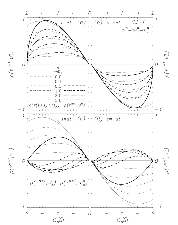
Figure 16: Cross-correlations between the configurational coordinate and the half-step velocities, $v_{\pm}^{n}$ for the GJ-I method with several different damping parameters. Thick curves represent the analytical result, Eq. (V.7.1) through a correlation expression similar to Eq. (50), as well as simulations of Eq. (94), which coincide with the analysis. Thin curves represent the continuous-time expectation, Eq. (5) with $s=\Delta{t}$. Simulation details given in Sec. III.5

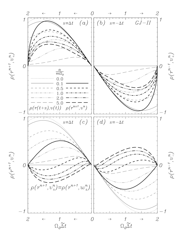
Figure 17: Cross-correlations between the configurational coordinate and the half-step velocities, $v_{\pm}^{n}$ for the GJ-II method with several different damping parameters. Thick curves represent the analytical result, Eq. (V.7.1) through a correlation expression similar to Eq. (50), as well as simulations of Eq. (94), which coincide with the analysis. Thin curves represent the continuous-time expectation, Eq. (5) with $s=\Delta{t}$. Simulation details given in Sec. III.5.

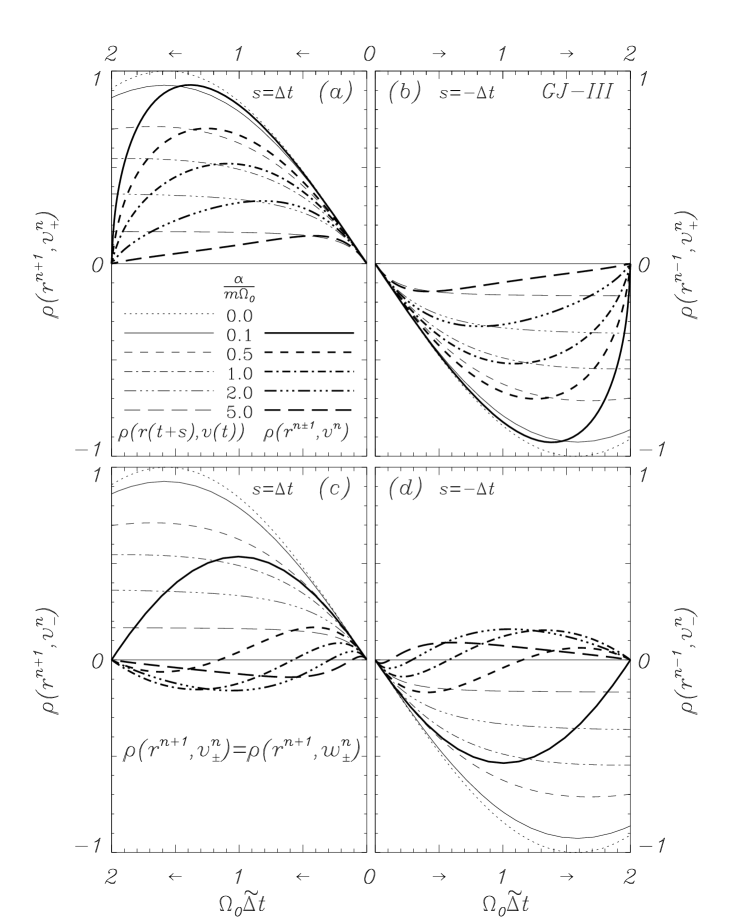
Figure 18: Cross-correlations between the configurational coordinate and the half-step velocities, $v_{\pm}^{n}$ for the GJ-III method with several different damping parameters. Thick curves represent the analytical result, Eq. (V.7.1) through a correlation expression similar to Eq. (50), as well as simulations of Eq. (94), which coincide with the analysis. Thin curves represent the continuous-time expectation, Eq. (5) with $s=\Delta{t}$. Simulation details given in Sec. III.5.

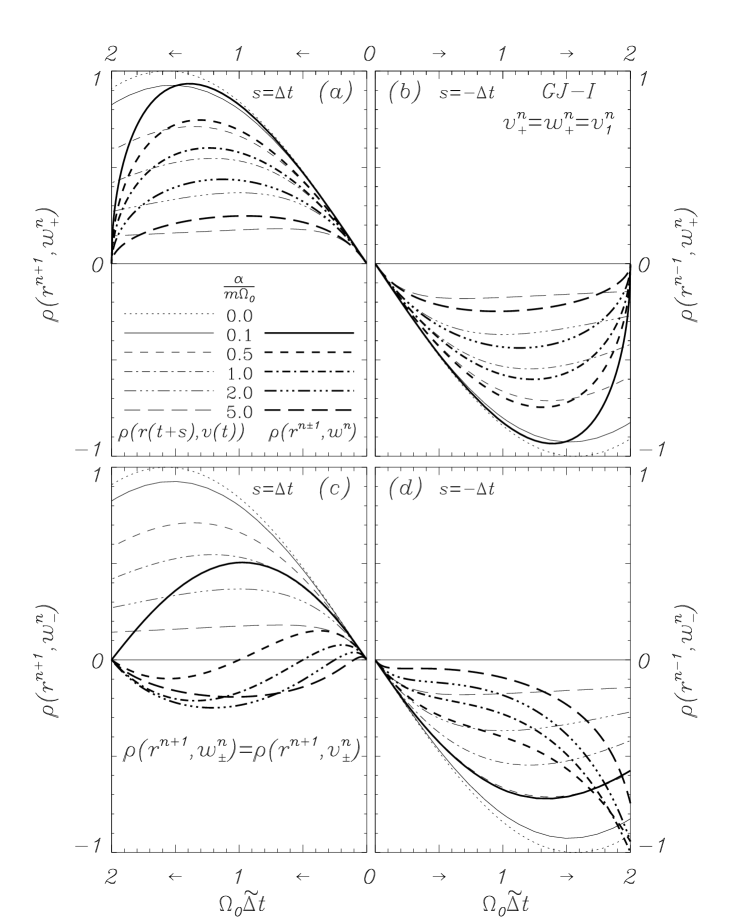
Figure 19: Cross-correlations between the configurational coordinate and the half-step velocities, $w_{\pm}^{n}$ for the GJ-I method with several different damping parameters. Thick curves represent the analytical result, Eq. (101) and (102) through a correlation expression similar to Eq. (50), as well as simulations of Eq. (100), which coincide with the analysis. Thin curves represent the continuous-time expectation, Eq. (5) with $s=\Delta{t}$. Simulation details given in Sec. III.5.

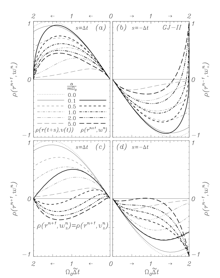
Figure 20: Cross-correlations between the configurational coordinate and the half-step velocities, $w_{\pm}^{n}$ for the GJ-II method with several different damping parameters. Thick curves represent the analytical result, Eq. (101) and (102) through a correlation expression similar to Eq. (50), as well as simulations of Eq. (100), which coincide with the analysis. Thin curves represent the continuous-time expectation, Eq. (5) with $s=\Delta{t}$. Simulation details given in Sec. III.5.

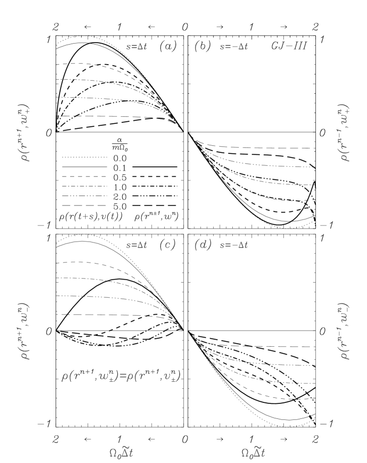
Figure 21: Cross-correlations between the configurational coordinate and the half-step velocities, $w_{\pm}^{n}$ for the GJ-III method with several different damping parameters. Thick curves represent the analytical result, Eq. (101) and (102) through a correlation expression similar to Eq. (50), as well as simulations of Eq. (100), which coincide with the analysis. Thin curves represent the continuous-time expectation, Eq. (5) with $s=\Delta{t}$. Simulation details given in Sec. III.5.

V.7.1 Enforcing correct drift and correlation anti-symmetry

Requiring that the on-site velocity has correct linear measure of drift velocity, Eq. (84a), and anti-symmetric covariance, Eq. (88), yields the finite difference coefficients

$$\mu_{2_{\pm}} = -(1-c_{2})\mu_{1_{\pm}}$$ (92a)

$$\mu_{3_{\pm}} = 1-(1+2c_{2})\mu_{1_{\pm}}$$ (92b)

$$\mu_{6_{\pm}} = 2c_{1}\mu_{1_{\pm}}-1\,,$$ (92c)

where $\mu_{1\pm}$ is given by the two options in Eq. (90), and $\mu_{4}$, $\mu_{5}$, and $\mu_{7}$ are given by Eqs. (76) and (78). The finite difference expression for the resulting velocity is thereby given from Eq. (69). However, a more condensed, and algorithmically favorable, expression can be written

$$v^{n}_{\pm} = 2\sqrt{c_{1}c_{3}}\mu_{1_{\pm}}v_{1}^{n}-\mu_{6_{\pm}}(\sqrt{c_{3}}v_{1}^{n-\frac{3}{2}}-\frac{c_{3}}{2m}\frac{\beta^{n-1}}{1-c_{2}})\,,$$

(93)

where $v_{1}^{n}$ and $v_{1}^{n-\frac{3}{2}}$ are given by Eqs. (LABEL:eq:OS_def_GJ) and (22). Including this pair of velocities into the GJ method, Eq. (24), can read

$$v^{n+\frac{1}{4}}\;=\;v_{1}^{n}+\sqrt{\frac{c_{3}}{c_{1}}}\frac{\Delta{t}}{2m}f^{n}$$

$$r^{n+\frac{1}{2}}\;=\;r^{n}+\sqrt{\frac{c_{3}}{c_{1}}}\frac{\Delta{t}}{2}v^{n+\frac{1}{4}}$$

$$v_{*}^{n-\frac{1}{2}} = \sqrt{c_{3}}v_{1}^{n-\frac{1}{2}}-\frac{c_{3}}{2m}\frac{1}{1-c_{2}}\,\beta^{n}$$

$$v_{1}^{n+\frac{1}{2}}\;=\;\sqrt{c_{1}}\,v^{n+\frac{1}{4}}+\frac{\sqrt{c_{3}}}{2m}\,\beta^{n+1}$$

$$v^{n+\frac{3}{4}}\;=\;\frac{c_{2}}{\sqrt{c_{1}}}\,v_{1}^{n+\frac{1}{2}}+\sqrt{\frac{c_{3}}{c_{1}}}\frac{1}{2m}\,\beta^{n+1}$$

$$r^{n+1}\;=\;r^{n+\frac{1}{2}}+\sqrt{\frac{c_{3}}{c_{1}}}\frac{\Delta{t}}{2}v^{n+\frac{3}{4}}$$

$$v_{1}^{n+1}\;=\;v^{n+\frac{3}{4}}+\sqrt{\frac{c_{3}}{c_{1}}}\frac{\Delta{t}}{2m}f^{n+1}$$

$$v_{\pm}^{n+1} = 2\sqrt{c_{1}c_{3}}\mu_{1_{\pm}}v_{1}^{n+1}-\mu_{6_{\pm}}v_{*}^{n-\frac{1}{2}}$$ (94b)

where only the numbered equations differ from Eq. (24), and where the single value, $v_{*}^{n-\frac{1}{2}}$, in Eq. (94) is used in Eq. (94b) to generate both on-site velocities, $v_{\pm}^{n+1}$.

The anti-symmetric covariance is in this case given by

$$\langle r^{n+1}v_{\pm}^{n}\rangle = -\langle r^{n-1}v_{\pm}^{n}\rangle$$

$$= 2c_{1}c_{3}\mu_{1_{\pm}}\Omega_{0}\Delta{t}\left(1-\frac{c_{3}}{4c_{1}}\Omega_{0}^{2}\Delta{t}^{2}\right)\frac{k_{B}T}{\sqrt{\kappa m}}\,,$$

which conforms to the continuous-time result, Eq. (3e), in the limit

$$\langle r^{n\pm 1}v_{-}^{n}\rangle \rightarrow \langle r^{n\pm 1}v_{+}^{n}\rangle\;\rightarrow\;\pm\Omega_{0}\Delta{t}\frac{k_{B}T}{\sqrt{\kappa m}}$$ (96)

for $\Omega_{0}\Delta{t}\rightarrow 0$.

Consistent with the comment above, we see that for the GJ-I method, $c_{3}=c_{1}$, which has $\mu_{1_{+}}=\frac{1}{2c_{1}}$, $\mu_{6}$ vanishes, and the algorithm simplifies considerably. In particular, the velocity measure $v_{+}^{n}$ coincides with $v_{1}^{n}$, leaving Eqs. (94) and (94b) superfluous if $v_{+}^{n}$ is the desired GJ-I choice for an on-site velocity with correct drift and anti-symmetric cross-correlation. Notice that, as predicted by Eqs. (83), due to the coefficient $\Gamma_{2}\neq 0$ of Eq. (81c), Figs. 13b-15b show that the velocities $v_{-}^{n}$ and $w_{-}^{n}$ can exhibit considerably smaller errors, especially for moderate damping, in the statistical kinetic measures than what is observed in Figs. 13a-15a for $v_{+}^{n}$ and $w_{+}^{n}$. This is consistent with the values $\mu_{1_{-}}<\mu_{1_{+}}$ of Eq. (90), as exemplified in Fig. 12, where it is obvious that typical methods will have $\mu_{1_{-}}\approx 0$ for $\frac{\alpha\Delta{t}}{m}\approx\frac{1}{2}$, in which case these on-site velocities measure the kinetic energy, temperature, and fluctuations (almost) correctly.

Figures 16-18 show the results of Eq. (V.7.1) through a correlation expression similar to Eq. (50) along with validating simulations of Eq. (94). These are indistinguishable. Also shown are the continuous-time expectations, Eq. (5) with $s=\Delta{t}$, which are in asymptotic agreement with the discrete-time results for $\frac{\alpha\Delta{t}}{m}\rightarrow 0$. As is the case for the comparable half-step velocity $v_{-}^{n+\frac{1}{2}}$ above, due to the related sign-change in $\mu_{1_{-}}$ seen in Fig. 12, the on-site velocity can exhibit peculiar behavior in its correlation with the trajectory. However, this may not necessarily imply irrelevance of this velocity, since a discrete-time velocity has no impact on the evolution of the simulation, and since the velocity is only used to extract information, which usually pertains to kinetic energy, kinetic fluctuations, and perhaps the correlations $\rho_{rv}(0)$ or $\rho_{E_{p}E_{k}}(0)$; all well represented by the velocity. In comparison, the velocity $v_{+}^{n}$ shows results much closer to the expected cross-correlation from continuous time.

V.7.2 Constraining $\mu_{6}=0$ $\Leftrightarrow$ $\mu_{7}=0$

The two conditions, Eqs. (84a) and (88), are generally mutually incompatible if $\mu_{6}=0$. Thus, a choice must be made about which of the two features is preferred.

Correct on-site drift (anti-symmetric cross-correlation is not enforced):
Interestingly, the condition Eq. (84a) with $\mu_{6}=0$, i.e., Eq. (LABEL:eq:vel_cond_6b) with $\mu_{6}=0$, yields precisely the same second order polynomial, Eq (89), as the one that appears when inserting the condition Eq. (88) into Eq. (LABEL:eq:vel_cond_6b). Thus, this velocity measure is also given by $\mu_{1_{\pm}}$ from Eq. (90) along with

$$\mu_{2_{\pm}} = 1-2\mu_{1_{\pm}}$$ (97)

$$\mu_{3_{\pm}} = \mu_{1_{\pm}}-1\,,$$ (98)

given by Eqs. (70) and (84a). The corresponding noise coefficients, $\mu_{4}$ and $\mu_{5}$, are given by Eqs. (76a) and (78), while $\mu_{7}=0$ follows from $\mu_{6}=0$ (see Eq. (76b)). The finite difference expression for the resulting velocity is thereby given from Eq. (69). However, a more condensed, and algorithmically favorable, expression can be written

$$w^{n}_{\pm} = 2\sqrt{c_{1}c_{3}}\mu_{1_{\pm}}v_{1}^{n}$$ (99)

$$-(2c_{1}\mu_{1_{\pm}}-1)(\sqrt{c_{3}}v_{1}^{n-\frac{1}{2}}-\frac{c_{3}}{2m}\frac{\beta^{n}}{1-c_{2}})\,,$$

where $v_{1}^{n}$ and $v_{1}^{n-\frac{1}{2}}$ are given by Eqs. (LABEL:eq:OS_def_GJ) and (22). Notice that, given $\mu_{1_{\pm}}$ being the same for the two velocities, $v_{\pm}^{n}$ and $w_{\pm}^{n}$, the leading factor ($2c_{1}\mu_{1_{\pm}}-1$) of the last term in Eq. (99) is given by the value for $\mu_{6_{\pm}}$ in Eq. (92c), even is $\mu_{6_{\pm}}=0$ for $w_{\pm}^{n}$. Including the pair of velocities, $w_{\pm}^{n}$, into the GJ method, Eq. (24), can read

$$v^{n+\frac{1}{4}}\;=\;v_{1}^{n}+\sqrt{\frac{c_{3}}{c_{1}}}\frac{\Delta{t}}{2m}f^{n}$$

$$r^{n+\frac{1}{2}}\;=\;r^{n}+\sqrt{\frac{c_{3}}{c_{1}}}\frac{\Delta{t}}{2}v^{n+\frac{1}{4}}$$

$$v_{1}^{n+\frac{1}{2}}\;=\;\sqrt{c_{1}}\,v^{n+\frac{1}{4}}+\frac{\sqrt{c_{3}}}{2m}\,\beta^{n+1}$$

$$v_{*}^{n+\frac{1}{2}} = \sqrt{c_{3}}v_{1}^{n+\frac{1}{2}}-\frac{c_{3}}{2m}\frac{1}{1-c_{2}}\beta^{n+1}$$

$$v^{n+\frac{3}{4}}\;=\;\frac{c_{2}}{\sqrt{c_{1}}}\,v_{1}^{n+\frac{1}{2}}+\sqrt{\frac{c_{3}}{c_{1}}}\frac{1}{2m}\,\beta^{n+1}$$

$$r^{n+1}\;=\;r^{n+\frac{1}{2}}+\sqrt{\frac{c_{3}}{c_{1}}}\frac{\Delta{t}}{2}v^{n+\frac{3}{4}}$$

$$v_{1}^{n+1}\;=\;v^{n+\frac{3}{4}}+\sqrt{\frac{c_{3}}{c_{1}}}\frac{\Delta{t}}{2m}f^{n+1}$$

$$w_{\pm}^{n+1} = 2\sqrt{c_{1}c_{3}}\mu_{1_{\pm}}v_{1}^{n+1}-(2c_{1}\mu_{1_{\pm}}-1)v_{*}^{n+\frac{1}{2}}\!\!\!,$$ (100b)

where only the numbered equations differ from Eq. (24), and where the single value, $v_{*}^{n+\frac{1}{2}}$, in Eq. (100) is used in Eq. (100b) to generate both on-site velocities, $w_{\pm}^{n+1}$.

We find the identity of the covariances

$$\langle r^{n+1}w_{\pm}^{n}\rangle = \langle r^{n+1}v_{\pm}^{n}\rangle\,,$$ (101)

where $\langle r^{n+1}v_{\pm}^{n}\rangle$ is given in Eq. (V.7.1). The complementary covariance is

$$\langle r^{n}w_{\pm}^{n+1}\rangle\;=$$ (102)

$$-\frac{1+2c_{1}\mu_{1_{\pm}}}{2}c_{3}\Omega_{0}\Delta{t}\left(1-\frac{c_{3}\mu_{1_{\pm}}}{1+2c_{1}\mu_{1_{\pm}}}\Omega_{0}^{2}\Delta{t}^{2}\right)\frac{k_{B}T}{\sqrt{\kappa m}}\,,$$

Clearly, the covariance between $r^{n}$ and $w_{\pm}^{n}$ is not, in general, anti-symmetric, even if, by design, $\langle r^{n}w_{\pm}^{n}\rangle=0$. The discrepancy in anti-symmetry is found from Eq. (87) to be

$$\langle r^{n}w_{\pm}^{n+1}\rangle+\langle r^{n+1}w_{\pm}^{n}\rangle = \frac{c_{3}}{2}\,\Omega_{0}\Delta{t}\,(2c_{1}\mu_{1_{\pm}}-1)\frac{k_{B}T}{\sqrt{\kappa m}}\,.$$

Given that Eq. (LABEL:eq:on-site_drift_asymmetry) shows a second order, in $\Delta{t}$, deviation from anti-symmetry of the covariance, and given Eqs. (96) and (102), we see that also the covariances in Eq. (102) conform to the continuous-time limit, Eq. (3e),

$$\langle r^{n\pm 1}w_{-}^{n}\rangle \rightarrow \langle r^{n\pm 1}w_{+}^{n}\rangle\;\rightarrow\;\pm\Omega_{0}\Delta{t}\frac{k_{B}T}{\sqrt{\kappa m}}$$ (104)

for $\Omega_{0}\Delta{t}\rightarrow 0$.

We again notice that the GJ-I method, where $\mu_{1_{+}}=\frac{1}{2c_{1}}$, is perfectly anti-symmetric in its cross-correlation between $r^{n}$ and $w_{\pm}^{n}$, even if this constraint has not been specifically enforced.

Correct on-site anti-symmetry (Correct drift velocity measure not enforced):
This velocity is characterized by Eq. (88) and, from Eq. (70),

$$\mu_{3} = -\mu_{1}-\mu_{2}\;=\;-c_{2}\mu_{1}\,,$$ (105)

where $\mu_{1}$ is found from inserting Eq. (88) into Eq. (81b) with $\mu_{6}=0$; thus

$$\mu_{1}^{2} = \frac{1}{4{c_{1}c_{3}}}\,.$$ (106)

The corresponding noise coefficients, $\mu_{4}$ and $\mu_{5}$, are given by Eqs. (76a) and (78). Notice that, since the correct drift measure is not enforced, Eq. (106) contains the possibility of a negative drift-velocity measure in response to a positive force. Clearly, $\mu_{1}$ should be chosen positive in this case.

The on-site velocity found here is the on-site velocity, $v_{1}^{n}$ from Eqs. (LABEL:eq:OS_def_GJ) and, e.g., (24) or (59), associated with the GJ methods of Ref. GJ . Reemphasizing previous comments, the GJ-I method, $c_{3}=c_{1}$, yields the correct drift velocity, even if not specifically enforced here.

Figures 19-21 show similar results as Figs. 16-18 described above, but for the velocities $w_{\pm}^{n}$. Shown are results of Eqs. (101) and (102) through a correlation expression similar to Eq. (50) along with validating simulations of Eq. (100). Numerical results are indistinguishable from the analytical predictions. The lack of anti-symmetry in the correlation is clearly visible for methods GJ-II, GJ-III, and GJ-I for $w_{-}^{n}$, whereas the results for GJ-I confirm that $v_{+}^{n}=w_{+}^{n}=v_{1}^{n}$ for this method, yielding the anti-symmetrical correlation behavior of $v_{1}^{n}$. We further observe that $\rho(r^{n+1},v_{\pm}^{n})=\rho(r^{n+1},w_{\pm}^{n})$. Also shown are the continuous-time expectations, Eq. (5) with $s=\Delta{t}$, which are in asymptotic agreement with the discrete-time results for $\frac{\alpha\Delta{t}}{m}\rightarrow 0$. As for the velocity $v_{-}^{n}$ above, the velocity $w_{-}^{n}$ can exhibit peculiar behavior in its correlation with the trajectory, in addition to the lack of anti-symmetry, given the related sign-change in $\mu_{1_{-}}$ seen in Fig. 12. The comments above for $v_{-}^{n}$ apply here as well; namely that the velocity has no impact on the evolution of the simulation, and that it is only used to extract information, which can very well be both useful and reliable for what is needed from a simulation.

VI Discussion

We have systematically identified viable options for correctly including one of the most basic, yet often overlooked, expectations for a velocity measure in Langevin simulations; namely the drift velocity. We have aimed to do this while also imposing correct Maxwell-Boltzmann statistics. The applied velocity ansatz for the analysis and development involves up to seven parameters consistent with the natural structure of stochastic Verlet-type algorithms, and the straight-forward, yet cumbersome, determination of these shows what options are possible. The expanded ansatz and analysis, compared to Ref. GJ , reaffirm that it is not possible to design a discrete-time, on-site velocity that produces correct, time-step independent statistics. However, we are able to define general-use, on-site definitions that have correct drift velocity as well as improved kinetic measures over previous expressions. For the half-step velocities, we have been able to identify specific measures that contain correct drift as well as correct Maxwell-Boltzmann statistics. These come in two forms, one using only one new stochastic value per degree of freedom per time step, and another using two (the latter was previously identified in a different form in Ref. Josh_3 ).

While not initially apparent, all the velocity definitions can be conveniently included into the existing GJ formalism as simple add-ons without significantly altering coding structure or complexity. Thus, the new velocity options can easily be implemented into existing codes, including LAMMPS Plimpton ; Plimpton2 , which is already offering the GJ-I method, for evaluation. We here give the complete set of new velocities embedded in the GJ method

$$v^{n+\frac{1}{4}}\;=\;v_{1}^{n}+\sqrt{\frac{c_{3}}{c_{1}}}\frac{\Delta{t}}{2m}f^{n}$$

$$r^{n+\frac{1}{2}}\;=\;r^{n}+\sqrt{\frac{c_{3}}{c_{1}}}\frac{\Delta{t}}{2}v^{n+\frac{1}{4}}$$

$$v_{1}^{n+\frac{1}{2}}\;=\;\sqrt{c_{1}}\,v^{n+\frac{1}{4}}+\frac{\sqrt{c_{3}}}{2m}\,\beta^{n+1}$$

$$v_{*}^{n+\frac{1}{2}} = \sqrt{c_{3}}v_{1}^{n+\frac{1}{2}}-\frac{c_{3}}{2m}\frac{1}{1-c_{2}}\beta^{n+1}$$ (107a)

$$v_{\pm}^{n+\frac{1}{2}} = \sqrt{c_{3}}\gamma_{1_{\pm}}v_{1}^{n+\frac{1}{2}}-\gamma_{3_{\pm}}v_{*}^{n-\frac{1}{2}}$$ (107b)

$$v_{d2}^{n+\frac{1}{2}} = \sqrt{c_{3}}v_{1}^{n+\frac{1}{2}}+\frac{\sqrt{c_{3}}}{\sqrt{2}m}\sqrt{\frac{1-c_{3}}{1-c_{2}}}\,\beta^{n+\frac{1}{2}}$$

$$v^{n+\frac{3}{4}}\;=\;\frac{c_{2}}{\sqrt{c_{1}}}\,v_{1}^{n+\frac{1}{2}}+\sqrt{\frac{c_{3}}{c_{1}}}\frac{1}{2m}\,\beta^{n+1}$$

$$r^{n+1}\;=\;r^{n+\frac{1}{2}}+\sqrt{\frac{c_{3}}{c_{1}}}\frac{\Delta{t}}{2}v^{n+\frac{3}{4}}$$

$$v_{1}^{n+1}\;=\;v^{n+\frac{3}{4}}+\sqrt{\frac{c_{3}}{c_{1}}}\frac{\Delta{t}}{2m}f^{n+1}$$

$$v_{\pm}^{n+1} = 2\sqrt{c_{1}c_{3}}\mu_{1_{\pm}}v_{1}^{n+1}-\mu_{6_{\pm}}v_{*}^{n-\frac{1}{2}}$$ (107d)

$$w_{\pm}^{n+1} = 2\sqrt{c_{1}c_{3}}\mu_{1_{\pm}}v_{1}^{n+1}-\mu_{6_{\pm}}v_{*}^{n+\frac{1}{2}}\,,$$ (107e)

where $\mu_{6_{\pm}}$ is given by Eq. (92c) for both Eqs. (107d) and (107e), per comment after Eq. (99). Incorporating the new velocities can equally well be accomplished within the compact form given in Eq. (25) by placing Eqs. (107a), (107b), and (107) after Eq. (25a); and Eqs. (107d) and (107e) after Eq. (24f). The half-step velocity $v_{d2}^{n+\frac{1}{2}}$ is simple to express and it is, from Figs. 8ab, 10, and 11, apparently well correlated with the configurational coordinate, especially for the GJ-I and GJ-III methods. The velocities that arise from the parameters $\gamma_{1_{-}}$ and $\mu_{1_{-}}$ are peculiar in both the leading coefficient and the cross correlations with configurational coordinate. However, the on-site velocities are perfectly uncorrelated with the trajectory at the same time, and the on-site velocities $v_{-}^{n}$ and $w_{-}^{n}$ can have significantly less error in kinetic measures, such as kinetic temperature and fluctuations, than other on-site velocities. It is therefore possible that these velocities can be useful for statistical simulations despite their unusual appearance. Particular interest may be given to the GJ-I method, for which the relationship $c_{3}=c_{1}$ significantly simplifies the method. Further, in that case, the velocity $v_{+}^{n}=v_{1}^{n}$. One particularly simple case is, again, GJ-I if one decides to use the half-step velocity $v_{d2}^{n+\frac{1}{2}}$ and not the on-site velocities, $w_{-}^{n}$ and $v_{-}^{n}$. This will eliminate the use for Eqs. (107a), (107b), (107d), and (107e) since in that case, $v_{+}^{n}=w_{+}^{n}=v_{1}^{n}$. The only cost from including $v_{d2}^{n+\frac{1}{2}}$ is the additional stochastic number, $\beta^{n+\frac{1}{2}}$.

The analysis in this work is linear in order to systematically formulate the developments. While it is likely that the analytically perfect behavior of these velocities may be perturbed by nonlinearities in the potential, we have not here performed evaluations of how the new velocity definitions perform for a variety of nonlinear and complex systems. Instead, we have provided the options and their rationale together with a convenient path to implement these options into existing codes. It is our hope that these methods for accurate kinetic measures can thereby be tested and evaluated broadly in many different contexts and applications.

VII Acknowledgments

The author is grateful.

VIII Data Availability Statement

The data presented and discussed in the current study are available from the author on reasonable request.

IX Funding and/or Competing Interests

No funding was received for conducting this study. The author has no relevant financial or non-financial interests to disclose.

References

• (1) M.P. Allen, D.J. Tildesley, Computer Simulation of Liquids, (Oxford University Press, Inc., 1989).
• (2) D. Frenkel and B. Smit, Understanding Molecular Simulations: From Algorithms to Applications, (Academic Press, San Diego, 2002).
• (3) D. C. Rapaport, The Art of Molecular Dynamics Simulations, (Cambridge University Press, Cambridge, 2004).
• (4) W. M. Hoover, Computational Statistical Mechanics, (Elsevier Science B.V., 1991).
• (5) A. Leach, Molecular Modeling: Principles and Applications, 2nd ed., (Prentice Hall: Harlow, England, 2001).
• (6) S. Toxsvaerd, Newtons discrete dynamics, Eur. Phys. J. Plus 135, 267 (2020).
• (7) For a review, see, e.g., E. Hairer, C. Lubich, and G. Wanner, Geometric numerical integration illustrated by the Størmer-Verlet method, Acta Numerica 12, 399 (2003).
• (8) L. Verlet, Computer experiments on classical fluids. I. Thermodynamical properties of Lennard-Jones molecules, Phys. Rev. 159, 98 (1967).
• (9) G. Strang, On the construction and comparison of dierence schemes, SIAM J. Num Analysis, 5, 506, 1968.
• (10) A. Ricci and G. Ciccotti, Algorithms for Brownian Dynamics, Mol. Phys. 101, 1927 (2003).
• (11) B. Leimkuhler and C. Matthews, Rational Construction of Stochastic Numerical Methods for Molecular Sampling, Appl. Math. Res. Express 2013, 34 (2012).
• (12) A. Brünger, C. L. Brooks, and M. Karplus, Stochastic boundary conditions for molecular dynamics simulations of ST2 water, Chem. Phys. Lett. 105, 495 (1984).
• (13) R. W. Pastor, B. R. Brooks, and A. Szabo, An analysis of the accuracy of Langevin and molecular dynamics algorithms, Mol. Phys. 65, 1409 (1988).
• (14) T. Schneider and E. Stoll, Molecular-dynamics study of a three-dimensional one-component model for distortive phase transitions, Phys. Rev. B 17, 1302 (1978).
• (15) W. F. van Gunsteren and H. J. C. Berendsen, Algorithms for macromolecular dynamics and constraint dynamics, Mol. Phys. 45, 637 (1982).
• (16) N. Grønbech-Jensen and O. Farago, Mol. Phys., A simple and effective Verlet-type algorithm for simulating Langevin dynamics, 111, 983 (2013).
• (17) L. F. G. Jensen and N. Grønbech-Jensen, Accurate configurational and kinetic statistics in discrete-time Langevin systems, Mol. Phys. 117, 2511 (2019).
• (18) N. Grønbech-Jensen, Complete set of stochastic Verlet-type thermostats for correct Langevin simulations, Mol. Phys. 118, e1662506 (2020).
• (19) J. Finkelstein, G. Fiorin, and S. Seibold, Comparison of modern Langevin integrators for simulations of coarse-grained polymer melts, Mol. Phys. 118, e1649493 (2020).
• (20) D. A. Sivak, J. D. Chodera, and G. E. Crooks, Time Step Rescaling Recovers Continuous-Time Dynamical Properties for Discrete-Time Langevin Integration of Nonequilibrium Systems, J. Phys. Chem. B 118, 6466 (2014).
• (21) J. Finkelstein, C. Cheng, G. Fiorin, B. Seibold, and N. Grønbech-Jensen, The Challenge of Stochastic Størmer-Verlet Thermostats Generating Correct Statistics, J. Chem. Phys. 153, 134101 (2020).
• (22) P. Langevin, On the Theory of Brownian Motion, C. R. Acad. Sci. Paris 146, 530 (1908).
• (23) W. T. Coffey and Y. P. Kalmykov, The Langevin Equation, 3rd ed., World Scientific, Singapore, 2012.
• (24) G. Parisi, Statistical Field Theory, (Addison-Wesley, Menlo Park, 1988).
• (25) W. C. Swope, H. C. Andersen, P. H. Berens, K. R. Wilson, A computer simulation method for the calculation of equilibrium constants for the formation of physical clusters of molecules: Application to small water clusters, J. Chem. Phys. 76, 637 (1982).
• (26) D. Beeman, Some multistep methods for use in molecular dynamics calculations, J. Comp. Phys. 20, 130 (1976).
• (27) O. Buneman, Time-reversible difference procedures, J. Comp. Phys. 1, 517 (1967).
• (28) R. W. Hockney, The potential calculation and some applications, Methods Comput. Phys. 9, 135 (1970).
• (29) M. Tuckerman, B.J. Berne and G.J. Martyna, Reversible multiple time scale molecular dynamics, J. Chem. Phys. 97, 1990 (1992).
• (30) N. Grønbech-Jensen, On the Application of Non-Gaussian Noise in Stochastic Langevin Simulations, J. Stat. Phys. 190, 96 (2023).
• (31) A. Papoulis, Probability, Random Variables, and Stochastic Processes, (McGraw-Hill, London, 1965).
• (32) See the LAMMPS manual http://lammps.sandia.gov/doc/Manual.pdf.
• (33) For a general description of pseudo-random generators and transformations of distributions, see, e.g., W. H. Press, S. A. Teukolsky, W. T. Vetterling, and B. P. Flannery, Numerical Recipes 3rd. ed. (Cambridge University Press, Cambridge, 2007).
• (34) J. Finkelstein, C. Cheng, G. Fiorin, B. Seibold, and N. Grønbech-Jensen, Bringing Langevin splitting methods into agreement with correct discrete-time thermodynamics, J. Chem. Phys. 155, 184104 (2021).
• (35) S. Plimpton, Fast parallel algorithms for short-range molecular dynamics, J. Comp. Phys. 117, 1 (1995).
• (36) A. P. Thompson, H. M. Aktulga, R. Berger, D. S. Bolintineanu, W. M. Brown, P. S. Crozier, P. J. in t Veld, A. Kohlmeyer, S. G. Moore, T. D. Nguyen, R. Shan, M. Stevens, J. Tranchida, C. Trott, S. J. Plimpton, LAMMPS – a flexible simulation tool for particle-based materials modeling at the atomic, meso, and continuum scales, Compute. Phys. Commun. 271, 108171 (2022).