n-th Root Optimal Rational Approximants
to Functions with Polar Singular Set
Abstract.
Let be a bounded Jordan domain and be its complement on the Riemann sphere. We investigate the -th root asymptotic behavior in of best rational approximants, in the uniform norm on , to functions holomorphic on having a multi-valued continuation to quasi every point of with finitely many branches. More precisely, we study weak∗ convergence of the normalized counting measures of the poles of such approximants as well as their convergence in capacity. We place best rational approximants into a larger class of -th root optimal meromorphic approximants, whose behavior we investigate using potential-theory on certain compact bordered Riemann surfaces.
Key words and phrases:
Rational approximation, meromorphic approximation, AAK approximation, Nehari approximation, weak distribution of poles, convergence in capacity2020 Mathematics Subject Classification:
30C15, 30E10, 31C40, 41A20, 41A25List of Symbols
General Point Sets:
unit circle, open unit disk, complex plane, and extended complex plane
circle and open disk of radius centered at the origin
Jordan curve, its interior domain, and the closure of its exterior domain in
Riemann Surfaces:
compact Riemann surface with natural projection
a connected component of homeomorphic to
the set of ramification points of a given Riemann surface
ramification order of a point on a Riemann surface
total number of sheets of
Classes of Functions:
continuous functions on a set
functions analytic in some neighborhood of
subclass of of functions multi-valued and quasi everywhere analytic off
subclass of of functions single-valued and quasi everywhere analytic off
class of functions quasi everywhere analytic on
subclass of approximated functions analytic on
algebraic polynomials of degree at most
monic algebraic polynomials of degree with all their zeros in
space of bounded holomorphic functions in
square integrable functions on the unit circle
essentially bounded functions on the unit circle
Hardy space of functions in with vanishing Fourier coefficients of negative index
Operators:
orthogonal projections from onto ,
Hankel operator from to ,
the -th singular number of
Potential Theory:
logarithmic capacity of
Greenian capacity of relative to
capacity of the condenser
Green function for with pole at
Green potential of the measure relative to
logarithmic potential of the measure
Green equilibrium distribution on a set relative to
balayage function of a superharmonic function relative to a set
balayage measure of a measure onto a set
lift of a measure on to
projection (pushforward) of a measure on to
fine boundary and closure of a set
base and the set of finely isolated points of a set
Various Symbols:
a conformal map from onto
collection of “branch cuts” for
“branch cut” of minimal Greenian capacity for
essential supremum norm on
error of best rational approximation of analytic on by functions in
1. Introduction
Rational approximation to holomorphic functions of one complex variable has long been a requisite chapter of classical analysis with notable applications to number theory [30, 56, 33], spectral theory [44, 26, 48] and numerical analysis [25, 32, 24, 17]. Over the last decades it became a cornerstone of modeling in Engineering [65, 66, 51, 1, 27], and it can also be viewed today as a technique to regularize inverse potential problems [22, 31, 4]. Finding best rational approximants of prescribed degree to a specific function, say in the uniform norm on a given set, seems out of reach except in rare, particular cases. Indeed, such approximants depend in a rather convoluted manner, both on the approximated function and on the set where approximation should take place. Accordingly, the constructive side of the theory has focused on estimating optimal convergence rates as the degree grows large and devising approximation schemes coming close to meet them [67, 7, 23, 62], or else studying the behavior of natural, computationally appealing candidate approximants like Padé interpolants and their variants [3, 61, 45, 38, 42].
When a function is holomorphic in some neighborhood of a continuum , the optimal speed of convergence for rational approximants on is at least geometric in the degree. Then, a coarse but manageable estimate of this speed proceeds via asymptotics of the -th root of the error in approximation by rational functions of degree . For functions analytically continuable off except over a polar set containing branchpoints (throughout polar means of logarithmic capacity zero), and provided that does not divide the extended complex plane, Gonchar and Rakhmanov constructed, using multipoint Padé interpolants and dwelling on work by the second author, a sequence of rational approximants whose -th root error on is asymptotically the smallest possible. They further showed that these interpolants converge in capacity on the complement of a compact set minimizing the capacity of the condenser under the constraint that the function is analytic off , and proved that the normalized counting measures of their poles converge to the condenser equilibrium distribution on [23]. It is remarkable that solves a geometric extremal problem from logarithmic potential theory, close in spirit to the Lavrentiev type [34], and that it depends merely on the set where approximation takes place, on the branchpoints of the approximated function and its monodromy, but nothing else. Such a structure emerges because only the -th root of the error is considered, rather than the error itself. Since then, it has been an open issue whether any -th root optimal sequence of approximants – in particular a sequence of best approximants – has the same behavior. The present paper answers this question in the positive, at least when the branchpoints are finite in number and order. In particular, our results connect, apparently for the first time, the singularities of best uniform approximants to those of the approximated function. We also address the case of no branchpoints, when the approximated function is analytic except over a polar set, in which the speed of best rational approximation on is known to be faster than geometric with the degree. We prove that -th root optimal approximants converge in capacity outside the singular set of the function, and that the “effective” poles converge in a sense to that set.
The gist of the paper becomes transparent upon observing that the behavior of rational approximants can be surmised when the function to be approximated extends analytically to a multiply-sheeted Riemann surface over the complex plane. As rational functions are single-valued, this topological discrepancy leads the approximants to mark out their domain of approximation by accumulating poles so as to form a cut, thereby preventing single-valued continuation in the limit. In the case of (diagonal) multipoint Padé interpolants, this cut has been characterized as being of smallest weighted capacity in a field that depends on the limiting distribution of the interpolation points, and poles asymptotically distribute according to the weighted equilibrium measure of that cut; moreover, the Padé interpolants converge in capacity on the extremal domain thus demarcated. This was established in [23], dwelling on the works [57, 58, 60, 61, 62] that deal with classical Padé interpolants and correspond to the zero field and unit weight; see also [46] for early developments along these lines, and [6] for applications to -best rational approximation on the circle. Subsequently, by choosing interpolation points adequately and performing surgery to eliminate spurious poles, the authors of [23] construct, on any continuum not dividing the extended plane and contained in the analyticity domain of a function indefinitely continuable except over a closed polar set containing branchpoints, a sequence of rational approximants converging uniformly to that function on as their degree grows large and whose -th root error has a liminf which is smallest possible, as well as a true limit. For this weakly optimal choice of interpolation points (meaning that the choice is optimal in the -th root sense), the cut of minimum weighted capacity is also the cut minimizing the condenser capacity of , as well as the cut of minimum Greenian capacity in the complement of . The smallest value for the limit of the -th root error is a simple, explicit function of this Greenian capacity, and the poles of the approximants thus constructed distribute asymptotically according to the Green equilibrium measure of that cut.
Now, assuming in addition that the branchpoints of the continuation off of the function to be approximated are finite in number and of algebraic type, we shall prove that any sequence of rational (or meromorphic) approximants of increasing degree whose -th root error on converges to the smallest possible limit – a fortiori every sequence of best approximants – has the same asymptotic distribution of poles as the particular sequence constructed in [23]. More precisely, if a function analytic in a simply connected neighborhood of a continuum in the extended complex plane is indefinitely continuable off that neighborhood except over a closed polar set containing finitely many branchpoints, all of algebraic type, then the normalized counting measures of the poles of any sequence of rational approximants of increasing degree with asymptotically optimal -th root error on do converge weak-star, as grows large, to the Green equilibrium distribution of the compact set of minimum Greenian capacity outside of which the function is single-valued; moreover, convergence holds in capacity everywhere off that compact set. Here, Green functions are understood with respect to the complement of the continuum where approximation takes place. Finally, if there are no branchpoints, that is, if the approximated function is single-valued and analytic on the extended complex plane except possibly over a closed polar set , then there are rational approximants converging on faster than geometrically with the degree. We shall prove that such sequences of approximants (as well as their meromorphic analogs) converge in capacity on the extended plane deprived from , and that retaining the singular part that comes close to generates new sequences of approximants, still converging faster than geometrically with the degree, while satisfying in addition that any weak-star limit point of the normalized counting measures of their poles is supported on .
Previously cited references, which deal with Padé or multipoint Padé interpolants, exploit the connection between denominators thereof and non-Hermitian orthogonal polynomials on a system of arcs encompassing the singular set of the interpolated function. Indeed, the core of the work in [60, 23] is to derive asymptotics of such polynomials on extremal systems of arcs like those constructed in [57, 58], so as to qualify the behavior of the poles of the interpolants when the degree grows large and deduce from it the desired convergence properties. Here, we proceed in the opposite direction: we assume that the optimal rate is met in the -th root sense and deduce from it the behavior of the poles. For this we cannot make use of orthogonal polynomials, and in fact it is not even known if interpolation takes place at all in the case of best approximants. However, the construction from [57, 58] will still be basic to our purposes.
This work was initiated jointly by the three authors in 2009, but the untimely passing away of the second one on April 22nd, 2013 prevented him from seeing its completion. Still, some fundamental ideas are his.
2. Preliminaries and Main Results
Given a function holomorphic in a neighborhood of a closed set , the error of approximation of on by rational functions of degree is
| (2.1) |
where stands for the supremum norm on and, for , we let be the class of rational functions of type with all their poles in . That is, if denotes the space of algebraic polynomials of degree at most and the monic polynomials of degree with all zeros in , then . It was shown by Walsh [67, 2], using interpolation techniques, that
| (2.2) |
where is any closed set disjoint from in the complement of which is holomorphic and denotes the capacity of the condenser . A definition of condenser capacity can be found in [55, Chapter VIII, Section 3]; for our purposes, it is enough to know that if is connected, then coincides with the Greenian capacity defined in Section A.4, see [55, Chapter VIII, Theorem 2.6 & Corollary 2.7] for this equivalence.
It is known that Walsh’s inequality (2.2) cannot be improved [37]. On the other hand, it was conjectured by Gonchar [28] and proven by Parfënov when is a continuum with connected complement [47] (also later by Prokhorov for any compact set [52]) that
| (2.3) |
Hence, has no limit in general as , and when the limit exists it cannot exceed the right-hand side of (2.3). For certain classes of functions and certain loci of approximation , it was nevertheless shown that does have a limit, which is equal to the right-hand side of (2.3). More precisely, let denote the space of functions holomorphic on a (variable) neighborhood of , and those functions continuable analytically into the complement of along any path that avoids some compact polar111see Section A.5 for a definition and basic properties of polar sets, that may be defined as sets of zero logarithmic capacity. subset of (which may depend on the function); we require in addition that this continuation is not single-valued, namely that there are paths with the same endpoints leading to different analytic branches. Now, when is a continuum that does not separate the plane and , it follows from work by the second author in [57, 58, 59] and it was explicitly stated by Gonchar and Rakhmanov in [23, Theorem 1′] that
| (2.4) |
where the infimum is taken over all compact sets such that admits a single-valued analytic continuation to .
Hereafter, we let be a Jordan curve with interior domain , and we put . In this setting , which is no loss of generality for a preliminary Möbius transform can ensure this; in contrast, our requirement that be a Jordan domain is a regularity assumption on the set where approximation takes place. Given , let be the collection of all compact sets such that , initially defined on , admits a single-valued analytic continuation to . It follows from [57, 58] that there exists , unique up to addition and/or removal of a polar set, with
| (2.5) |
We can and will normalize to be the smallest possible, i.e., we make it the intersection of all for which is minimal, see [58]. As , in light of equation (2.4), our main goal is to investigate the asymptotic behavior of sequences of rational functions of type meeting this optimal -th root rate:
| (2.6) |
We call any such sequence a sequence of -th root optimal rational approximants to on . In order to study , we are led to consider more general sequences of meromorphic approximants of the form , where is holomorphic in and continuous on , see Section 2.3 for the definitions. Even though best meromorphic approximants may look less natural than rational ones, they make contact with both the spectral theory of Hankel operators (through AAK theory) and Green potentials (because they generate errors with constant modulus on ), while remaining essentially equivalent to rational approximants as far as -th root error rates are concerned [47]. This is why -th root optimal meromorphic approximants (meeting (2.6) in place of ) are of principal importance in our study. Yet, the potential-theoretic tools on Riemann surfaces that we use only allow us to handle compact surfaces so far, and this induces some finiteness conditions on the functions from the class that we can deal with. These are set forth in the next section.
2.1. Class of Approximated Functions
We consider functions in such that
-
(i)
they can be continued into along any path originating on that stays in while avoiding a closed polar subset of (which may depend on the function);
-
(ii)
they are not single-valued, meaning there are continuations along at least two paths as in (i) with the same initial and terminal points that lead to distinct function elements, but still they are finite-valued in that the number of such function elements lying above a point of is uniformly bounded (the bound may depend on the function);
-
(iii)
their number of branchpoints (points in any neighborhood of which some analytic continuation along a closed path in encircling that point while avoiding the exceptional polar set leads to a different function element) is finite.
In view of (i) and (ii), such functions lie in . Note that (iii) is not superfluous, for there are functions meeting (i) and (ii) with infinitely many branchpoints. For instance, an open Riemann surface made of two copies of , glued along a sequence of disjoint cuts in shrinking to the point , has projection a two sheeted covering with infinitely many branchpoints of order . As carries a holomorphic function assuming more than one value on for not a critical value of [18, Theorem 26.7], we deduce on putting and that each branch of is of the announced type.
We formalize (i), (ii) and (iii) as follows. Let be an auxiliary algebraic Riemann surface, whose set of ramification points lies on top of . That is, there exists an irreducible polynomial in two variables , of degree at least 2 in , such that and all branchpoints of the algebraic function lie in . We denote by the natural projection , and we let be the (open) Riemann surface defined as
here and below, whenever it causes no confusion, we use letter to denote both points in and on . Clearly, the ramification points of and are identical: . Let us denote by the closure of in , and define a class of functions by
| (2.7) |
In (2.7), we wrote for the singular set of on but it would have been more appropriate to write , as the complete Riemann surface of could be significantly larger than and its singular set bigger than . Since all ramification points of lie on top of , the simple-connectedness of implies that the preimage consists of finitely many homeomorphic copies of under ; we generically denote by such a copy, so that is a homeomorphism. Then, denoting with a subscript the restriction to a set , the class of functions that we study is defined as
| (2.8) |
From (2.7) and (2.8), one sees that and members of meet (i), (ii), (iii). Conversely, when satisfies (i), (ii) and (iii), one can check that . Indeed, if is the closed polar subset of defined by (i), we get from (ii) because is connected, see Section A.5, that the number of sheets of the Riemann surface of above is a finite constant, say . Therefore, since the branchpoints are finitely many by (iii), the algebraic surface can be constructed by a classical glueing process described in Section 3.2. The fine point, when applying to the present case this familiar procedure based on glueing pairwise in a certain order the banks of copies of a system of cuts joining the branchpoints, is that any two points of can be joined by a smooth simple arc entirely contained in , except for its endpoints if they lie in . It is so because is a connected open set and each point of is the center of a circle of arbitrary small radius contained in , as well as the endpoint of a segment contained in (that may even be chosen to have quasi-any direction). These properties hold because is polar, and therefore thin at each point of , see Section A.6.
We also consider functions in meeting (i) but not (ii). These are analytic and single-valued in , where is closed and polar, i.e., there are no branchpoints. This case complements the previous one on putting and omitting the last requirement in (2.7); we denote the corresponding class of functions by . Since when is polar, see Section A.4, we get from (2.3) and (2.2) that
| (2.9) |
That is to say, some sequence , , of rational functions, converges faster than geometrically towards on as the degree grows large, meaning that
| (2.10) |
We call any such sequence a sequence of -th root optimal rational approximants to on .
2.2. Optimal Rational Approximants
Notions of potential theory in and play a fundamental role in what follows, and the reader might want to consult Appendix A for a comprehensive account thereof. Let us here recall the definition of Green potentials and Green equilibrium distributions.
The Green function of the domain with pole at is the unique non-negative harmonic function in , with logarithmic singularity at , whose largest harmonic minorant is zero. The Green potential of a positive Borel measure in is . Putting for the total mass of , the Greenian capacity (in ) of a Borel set is defined by
| (2.11) |
the infimum above is taken over all probability Borel measures supported on . For any set , the outer Greenian capacity of in is defined as , where the infimum is taken over all open sets in (using again the symbol causes no confusion for the outer Greenian capacity is known to coincide with the Greenian capacity on Borel sets). Polar subsets of are those whose outer Greenian capacity is . If is a non-polar compact subset of , then there exists a unique Borel probability measure supported on , called the Green equilibrium distribution on relative to , such that . It is characterized by the property that its Green potential is bounded on and equal to its maximum (which is then necessarily ) quasi everywhere (that is, up to a polar set) on . To recap:
| (2.12) |
where the last inequality follows from the (generalized) maximum principle for harmonic functions.
We are concerned with two types of asymptotics for sequences of rational approximants: the weak∗ behavior of the normalized counting measures of their poles, and the convergence in capacity of the functions themselves. More precisely, given a rational function of type , we define
| (2.13) |
where each pole appears in the sum as many times as its order. Equivalently is the distributional Laplacian , with the denominator of an irreducible form of . One says that a sequence of finite Borel measures on converges weak∗ to a measure , denoted as
if for every continuous compactly supported function on . We further say that a sequence of functions converges in Greenian capacity to a function on a set if
| (2.14) |
for each and every compact ; we denote this claim by in . The convergence (2.14) is said to hold at a geometric rate if we can replace in (2.14) by for some positive ; the convergence rate is called faster than geometric if (2.14) holds with replaced by for any .
Theorem 2.1.
Let be a Jordan curve, its interior and the complement of on the Riemann sphere. Given , let be such that (2.5) holds and be a sequence of -th root optimal rational approximants to on , as defined in (2.6). Then,
| (2.15) |
where is the normalized counting measure of the poles of and is the Green equilibrium distribution on relative to . Furthermore, it holds that
| (2.16) |
where is the Green potential of in .
Remark 2.2.
Theorem 2.1 and equation (2.12) imply that -th root optimal rational approximants converge to in capacity in , at a geometric rate equal to pointwise. In fact, as shown in Section 3.11, convergence in Greenian capacity in and uniform convergence on , along with the limiting behavior (2.15) for the poles, together imply the seemingly stronger convergence in logarithmic capacity on , at a geometric rate which is pointwise no slower than the previous one. Here, convergence in logarithmic capacity is defined as in (2.14), except that the logarithmic capacity replaces the Greenian one, see Section A.4 for a definition of logarithmic capacity. This remark equally applies to the forthcoming Theorem 2.5, as well as to Theorems 2.3 and 2.6 in which gets replaced by a polar set and convergence takes place at faster than geometric rate. Moreover, if in Theorem 2.5 the error is asymptotically circular on , namely if (in particular when are their own Nehari modifications, see Section 3.3), then one can draw the more precise conclusion that the exact pointwise rate of geometric convergence of to in logarithmic capacity on is the same as in Greenian capacity on , namely .
In view of its importance, let us describe in greater detail the set . As mentioned before, the problem of finding elements of minimal capacity in was extensively studied by the second author [57, 58, 59]. The existence of such sets for was proven in [57], and one can choose so that for any with , which makes unique [58]. The topological structure of was investigated in [59], where it is shown that
| (2.17) |
where the are open analytic arcs, comprises the endpoints of the arcs , and is a subset of the singular set of in (the singular set consists of those points in to which some continuation of from has a singularity). As soon as , the set is polar by definition. To understand this decomposition better when , let so that . Then possesses a single-valued continuation into with singular set , consisting of polar and essential singularities (but no branching singularities). If , are as in (2.8) and is the connected component of containing in its boundary, then we can further decompose:
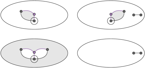
That is, is the set of “active” branchpoints of , i.e., branchpoints that can be reached by continuation of from into , as opposed to those points in that cannot be so reached. Also, each is an endpoint of at least three arcs , and generically possesses analytic continuations to from any direction within (unless by chance is a singularity of as well), see Figure 1. As is finite, so is the collection in cases that we consider.
For , Theorem 2.1 asserts two things: (i) the weak∗ convergence of to whenever is an -th root optimal sequence of rational approximants to on , and (ii) the convergence in capacity of to at a geometric rate on . If now and is a sequence of -th root optimal rational approximants to on , i.e., a sequence meeting (2.10) and thus converging faster than geometrically to on , then we shall see that converges in capacity to at faster than geometric rate in . However, one can no longer expect a specific behavior of in this case, for if is a sequence in that converges to zero faster than geometrically on , then is again a sequence of -th root optimal rational approximants to on , whereas the weak∗ limit points of can be arbitrary amongst positive measures of mass at most on . Thus, faster than geometric convergence does not qualify rational approximants enough to imply much on the behavior of their poles. Still, those poles of that stay away from the singular set of cannot account for the rate of convergence. This is made precise in the following result, which complements Theorem 2.1 in the case of no branchpoints.
Theorem 2.3.
Let , and be as in Theorem 2.1. Given , let be a sequence of rational functions of type meeting (2.10). Then, it holds that
at faster than geometric rate, where a closed polar set outside of which is analytic and single-valued. Moreover, for any neighborhood of there is a sequence , , , such that the poles of are among the poles of lying in and
| (2.18) |
Using neighborhoods shrinking to and a diagonal argument, Theorem 2.3 yields a corollary of independent interest.
Corollary 2.4.
If and a closed polar set outside of which is analytic and single-valued, then there is a sequence of rational functions , , converging faster than geometrically to on , and such that every weak∗ cluster point of the sequence of normalized counting measures of the poles is supported on .
2.3. Optimal Meromorphic Approximants
Let denote the space of bounded analytic functions on and the subspace of those extending continuously to . When is rectifiable each has a non-tangential limit almost everywhere on with respect to arclength, that we still call , and putting for the essential supremum norm on (with respect to arclength) it holds that [12, Theorems 10.3 & 10.5]. When is a non-rectifiable Jordan curve, however, limiting values of -functions on generally exist at sectorially accessible points only, and such points may reduce to a set of zero linear measure [41]. This will force us into a somewhat careful discussion of meromorphic approximants. Remember the set of monic polynomials of degree whose zeros belong to , and put
That is, is the set of meromorphic function with at most poles in that are bounded near , and is the subset of those extending continuously to . We shall say that is a sequence of -th root optimal meromorphic approximants to on if and
| (2.19) |
Any sequence of -th root optimal rational approximants is a particular sequence of -th root optimal meromorphic ones, by (2.6). When is rectifiable, Corollary 2.7 to come will entail that in (2.19) the condition can be traded for the seemingly weaker requirement . However, it is important to require that when is not rectifiable, for otherwise the left-hand side of (2.19) may no longer make sense for the essential supremum norm (with respect to arclength) and the considerations below would not apply. In his proof of (2.3), Parfënov [47] has shown that the limit inferior of is the same as the one of the -th root of the error in best meromorphic approximation, see (2.22) for a definition of best (not just -th root optimal) meromorphic approximants. Hence, in light of (2.6), replacing rational approximants with meromorphic ones does not improve the rate of decay of the -th root error, and -th root optimal meromorphic approximants to functions in could be defined with the limit superior and the inequality sign replaced by a full limit and the equality sign in (2.19).
Theorem 2.5.
Let us reiterate that -th root optimal rational approximants are just an instance of -th root optimal meromorphic approximants, and therefore Theorem 2.1 is a special case of Theorem 2.5.
When , we define meromorphic approximants in a manner similar to (2.19) but this time with an eye on (2.9). Namely, we say that is a sequence of -th root optimal meromorphic approximants to on if and
| (2.20) |
The following complements Theorem 2.5 in the case of no branchpoints, and subsumes Theorem 2.3.
Theorem 2.6.
Besides best rational approximants, a noteworthy instance of -th root optimal meromorphic approximants are the AAK (short for Adamyan-Arov-Krein) approximants. These are best meromorphic approximants with at most poles. Specifically, consider the following (Nehari-Takagi) problem: given , find such that
| (2.21) |
If , then (2.21) reduces to the question of best analytic approximation of bounded functions on the unit circle by elements of , which is the so-called Nehari problem named after [43] (that deals with an equivalent issue). It is known that always exists and that it is unique when lies in , see [48, Chapter 4]. Moreover, if is Dini-continuous on , then is continuous on . Indeed, if we write where and , we see that must be the best Nehari approximant to , which is Dini-continuous on , and the claim follows from [9]. When is a rectifiable Jordan curve, one can readily replace by in (2.21) and carry over to all the properties of best meromorphic approximants on by conformal mapping. When is non-rectifiable, the very existence of approximants depends on the analyticity of on , and follows from the proof of the next corollary to Theorem 2.5.
Corollary 2.7.
Much interest in best meromorphic approximants stems from their striking connection to operator theory. Denote by the space of square integrable functions on , and let be the Hardy space of functions whose Fourier coefficients with negative index do vanish. It is known that can be identified with (non-tangential limits on of) analytic functions in whose -means on circles centered at the origin are uniformly bounded, see [12, Theorem 3.4]. Set to be the orthogonal complement of , which is the Hardy space of -functions whose Fourier coefficients with nonnegative index are equal to zero. The latter can be identified with functions analytic in that vanish at infinity, and whose -means with respect to normalized arclength on circles centered at the origin are uniformly bounded. Let be the orthogonal projection. Given , one defines the Hankel operator with symbol to be
| (2.23) |
For a non-negative integer, let be the -th singular number of the operator , that is , where the infimum is taken over all operators of rank at most and stands for the operator norm. Then, one has that
| (2.24) |
If, in addition, , then is compact so that is the -st eigenvalue of when these are arranged in non-increasing order, and (2.24) becomes a pointwise equality:
| (2.25) |
Moreover, if is an -st singular vector of , i.e., an eigenvector of with eigenvalue , then is explicitly given in terms of and by the formula
| (2.26) |
Though not obvious at first glance, the right-hand side of (2.26) is independent of which -th singular vector is chosen and it has constant modulus on , in accordance with (2.25). The next corollary, of independent interest, follows from (2.25), (2.19), (2.9), and Theorems 2.5–2.6.
Corollary 2.8.
Let be the Hankel operator with symbol . Then, it holds that
Moreover, if , then the above limit is equal to .
3. Proof of Theorem 2.5
3.1. Existence of Best Meromorphic Approximants
Below, we establish the existence and uniqueness part of Corollary 2.7, along with the assertion that may replace when is rectifiable. The rest of the corollary will follow from Theorem 2.5 upon conclusion of its proof.
Let be a conformal map. Since is a Jordan domain, extends to a homeomorphism from to by Carathéodory theorem [50, Section 2]. Let , , and be as defined after Corollary 2.7 and , be the orthogonal projections. If we pick a continuous function on , then is continuous on and, in particular, it lies in . Set and , so that and . Since is the identity operator, it holds that
| (3.1) |
Now, if , then is holomorphic in and continuous in , for close enough to . Hence, the right-hand side of (3.1) is holomorphic in with uniformly bounded -means on circles centered at the origin, while the left-hand side lies in and both sides have the same non-tangential limit on . By an easy variant of Morera’s theorem [21, Chapter II, Exercise 12], the function equal to for and to for is holomorphic across , in particular extends analytically across and extends continuously to . Then, as described after (2.21), the best meromorphic approximant to exists and is unique, moreover it is readily checked that is equal to the sum of (a member of ) and of the best approximant to from , which lies in because is analytic across and so is a fortiori Dini-continuous on ; hence, we get that . If now , then and
by definition of . As , it is the unique best meromorphic approximant to we are looking for. The previous argument also shows that, when , the best meromorphic approximant to necessarily belongs to . Because composition with is an isometric isomorphism (understood with respect to arclength measure) when is rectifiable, one can equivalently use instead of in definition (2.22).
3.2. Reduction to the Unit Disk
Let be a compact subset of . Since Green potentials are non-negative superharmonic functions whose largest harmonic minorant is zero, while a characteristic property of Green equilibrium potentials is to be constant quasi everywhere on the support of their defining measure while being no greater than this constant everywhere in the domain, it holds that
where is a conformal map, see (2.12) as well as Sections A.3 and A.4. One has in this case that , the pushforward of under . Hence, we get that
where the weak∗ convergence is understood for . Furthermore, by conformal invariance, a sequence of functions converges in Greenian capacity to a function in if and only if the functions converge in Greenian capacity to the function in .
Let now and be as in Section 2.1. Denote by the number of sheets of , so that a generic point in has preimages under the natural projection . Let be a smooth oriented Jordan arc joining two points of while passing through all others exactly once. Constructing is tantamount to enumerating the points of . Write where each connects exactly two points in . The surface can be realized as copies of , suitably glued to each other along the banks of the cuts in each copy (the glueing rule can be encoded, for example, as a collection of 4-tuples telling one that the left and right banks of the cut in need to be glued to the right bank of the cut in and the left bank of the cut in respectively, see [40] for a discussion of Hurwitz’s theorem). Using the same gluing rule, we can construct another -sheeted surface out of the domains . The map can then be lifted to a conformal map for which , , where is the natural projection.
Let and be as in (2.8) and (2.7). Clearly , and the surface can be constructed by gluing copies of to along the homeomorphic copies of that comprise the boundary of . Argueing as we did after (3.1), we find that lies in with the corresponding given by , where . Note that the conformal equivalence of Greenian capacities implies that . Hence, if is an -th root optimal sequence of meromorphic approximants of in as defined in (2.19), then is an -th root optimal sequence of meromorphic approximants to on and
| (3.2) |
Therefore, it is sufficient to study the asymptotic behavior of as well as the limit distribution of poles of . That is, it is enough to prove Theorem 2.5 on the unit disk.
3.3. Nehari Modifications
For and , let be the best holomorphic (Nehari) approximant of in . That is, , and . Let us set
| (3.3) |
and call the Nehari modification of . The discussion after (2.21) shows that lies in . Indeed, we may write with and . Then, one can readily check that . As is analytic across and in particular Dini-continuous there, it follows that belongs to and so does .
Since and lies in , the sequence is one of -th root optimal meromorphic approximants to , whenever is such a sequence. It is beneficial for us to consider Nehari modifications because they enjoy the additional property that the error they generate has constant modulus on , i.e., it follows from (2.24) that
| (3.4) |
We claim that it is enough to prove Theorem 2.5 for Nehari modifications only, as we now show.
Assume that Theorem 2.5 holds for . As the poles of and are the same, this automatically yields the statement about weak∗ convergence of the counting measures of the poles. Moreover, given and a compact set, let us put
Define analogously. According to our assumption it holds that
| (3.5) |
and we need to show that (3.5) holds with replaced by . Given , define
where . Since is analytic in , we get from the maximum modulus principle and the triangle inequality that for . Since , relation (2.19) implies that
for all large enough. Hence, by the previous estimates, it holds for all such and that
In particular, for any , there exists depending on and such that
| (3.6) |
for all and . Therefore, we get from the triangle inequality that
for all . The above inclusion clearly yields that (3.5) holds with replaced by for . As , , and were arbitrary, the claim follows.
3.4. Notation
We fix and, with a slight abuse of notation, we keep denoting by the corresponding function in (that was denoted by in (2.8)). Take to be a sequence of -th root optimal meromorphic approximants of and let be the sequence of corresponding Nehari modifications. Since is also -th root optimal, it holds that
| (3.7) |
see the discussion after (2.19). We shall need an exhaustion of by open sets with “nice” boundaries. That is, we consider a sequence of open sets such that
| (3.8) |
and each , when viewed as an open subset with compact closure of , is regular for the Dirichlet problem, see Section A.7. We will require in addition that for some Radon measure on that will be specified at the beginning of Section 3.5 (a Radon measure is a positive Borel measure which is finite on compact sets). To design regular that meet (3.8) is possible because , being compact in , is a countable intersection of compact sets with smooth boundary. Indeed, there is a smooth function on such that is the zero set of and outside a compact neighborhood of , hence we can pick to be the sublevel set , where a sequence of regular values of tending to 0 (almost every positive number is a regular value by Sard’s theorem). In fact, using smooth partitions of unity and local coordinates, existence of such quickly reduces to the corresponding issue in Euclidean space, where it follows easily from a combination of [63, Chapter VI, Theorem 2] and [68, Theorem I] (this result is named after H. Whitney). Furthermore, since the sets are compact for and small enough, . So, for at most countably many positive , and we can assume that chosen above are not such values. The domains thus constructed satisfy all our requirements.
Let be a subdomain of or . Given a Borel measure on , we denote the Green potential of relative to by , see Section A.2. Hereafter, every measure is Borel unless otherwise stated. If is a measure on a Borel set containing , we write for simplicity to mean . Conversely, for a measure on a Borel set , we still denote by the measure on mapping a Borel set to , and write for its potential. When is a (possibly infinite) sum of Dirac delta measures, we put
| (3.9) |
to stand for the corresponding generalized Blaschke product, where is a complexified Green potential, i.e., it is locally holomorphic in and . If , which can happen when the points accumulate in or to the boundary sufficiently slowly, then is identically zero. Otherwise, is well defined up to a unimodular constant (because the periods of a conjugate function of are integral multiples of by Gauss’ theorem), holomorphic in , unimodular quasi everywhere on (everywhere if the latter is regular and the points are finite in number), and it vanishes only at the points (with multiplicities represented by repetition).
3.5. Stripped Error of Approximation
We shall study the asymptotics of the error functions . In this section, we strip off their poles and zeros to take logarithms and obtain harmonic functions whose limiting behavior we then investigate. To this end, we set
| (3.10) |
where are the poles of and the zeros of , with multiplicities counted by repetition. Before we proceed, let us specify the measure appearing in the definition of the exhaustion in the previous subsection. To this end, recall that on a locally compact space , a sequence of Radon measures converges vaguely to a Radon measure if for every in , the space of continuous functions with compact support on endowed with the -norm. Moreover, if the measures are locally bounded on , then they do contain a vaguely convergent subsequence, see for example [14, Theorem 1.41] for an argument on which is applicable to any -compact locally convex space222Vague convergence is called weak convergence in [14].. Hence, since the measures have mass at most 1, we get if is locally bounded along some sequence of integers that there exists a subsequence , a measure on and a measure on such that and converge vaguely to and , respectively, along ; if the measures have no locally bounded subsequence, i.e., if there exists a compact set such that as , then we put and we only require the vague convergence along . In any case we take to be , where is the lift of to defined via (A.33).
Using (3.9), we define Blaschke products vanishing at the poles of and the zeros of . Namely, we put
These functions are not identically zero, as the number of poles of is at most while the number of zeros of in each is finite. To see the latter point, recall from (3.4) that is constant on , hence the error can be meromorphically continued across by reflection. It implies that can be meromorphically continued across and this continuation is necessarily analytic in some neighborhood of . Thus, is analytic in a neighborhood of by the analyticity of there, so the zeros of can only accumulate on and not on . Thus, there are at most finitely many of them in each .
Using these Blaschke products, we define
| (3.11) |
which is harmonic in . Recall that superharmonic functions on a hyperbolic Riemann surface are either identically or finite quasi everywhere, and any two of them that coincide almost everywhere (with respect to Lebesgue measure in local coordinates) are in fact equal (the weak identity principle), see Section A.1.
Lemma 3.1.
There exist a subsequence and a non-negative superharmonic function on such that
| (3.12) |
locally uniformly in , for any subsequence . If is finite quasi everywhere, then one has a decomposition
| (3.13) |
where is a finite positive Borel measure supported on and is a non-negative harmonic function on .
Proof.
The regularity of implies that for , and likewise for on . In particular we get that
by the maximum modulus principle for -functions. Set be the Hankel operator with symbol , see (2.23). It follows from the definition of the singular values, (2.24), and (3.3) that . Since the norms tend to zero by assumption, we get that
| (3.14) |
for some constant that depends only on and the sequence . Thus, we get from the maximum principle for harmonic functions that
| (3.15) |
Set . Proceeding inductively on , we deduce from (3.15) that the sequence is uniformly bounded above in and therefore, by Harnack’s theorem, see Section A.1, there exists a subsequence such that
| (3.16) |
locally uniformly in , where is either identically or a non-positive harmonic function. Define to be the diagonal of the table ; that is, the -th element of is the -th element of . Then, (3.16) holds along for each .
Additionally, it follows from the maximum modulus principle for holomorphic functions that
Therefore, we get from (3.11) and (3.15) that for when . Thus, if a finite limit exists for some index , then it exists for all . Hence, either the functions converge to as locally uniformly in each , in which case for all , or else the functions are finite and harmonic for all large enough.
If for all , select for each some such that for and all ; we may require in addition that for . Then (3.12) holds with and .
If on the contrary the functions are finite, they form an increasing sequence on for and fixed . As they are non-positive, they converge locally uniformly in to a non-positive harmonic function, say , again by Harnack’s theorem. Since is a closed polar set and is non-negative, it follows from the Removability theorem, see Section A.5, that extends to a superharmonic function on that we keep denoting by . Because is superharmonic on and harmonic on , its Laplacian is a negative Radon measure supported on , which is necessarily finite since is compact. Thus, by the Riesz representation theorem, see Section A.3, equation (3.13) takes place with the largest harmonic minorant of .
Given , choose such that for and all . Define , where we again additionally require that . Given a compact set and , we can pick large enough that
Then, it follows from the last two inequalities that for and any . Since and were arbitrary, this finishes the proof of (3.12). ∎
Proof.
Let , with close enough to that for each . It follows from the proof of Lemma 3.1 that as , locally uniformly in . Given a connected component of , let be its harmonic measure, see Section A.9. Then
| (3.18) |
for any and , see (A.28). It then follows from the monotone convergence theorem that we can take in (3.18). Recall that is analytic across and hence is non-vanishing there except perhaps for finitely many zeros counting multiplicities. Since is harmonic in , is continuous on , and is equal to on (i.e., it is continuous on except perhaps for finitely many logarithmic singularities), we get from (3.18) and (A.28) that
By (3.7) the pointwise limit of on is minus the right-hand side of (3.17) except perhaps for a finite subset of , where may go to zero, contained in
As does not charge polar, thus finite sets, the convergence in fact holds almost everywhere with respect to for each fixed . So, if we can justify the second equality in the following relation:
| (3.19) |
we shall get that solves a Dirichlet problem on with boundary data equal to on , and to the negative of the right-hand side of (3.17) on . As such, must extend continuously to where it is equal to the boundary data, since is non-thin at any of its points. Subsequently, as converges to locally uniformly on (see the proof of Lemma 3.1), passing to the limit in the leftmost and rightmost sides of (3.19) when yields that extends continuously to with values given there by the right-hand side of (3.17). This will give us the desired conclusion, because is compactly supported in and therefore continuously extends by zero to since is regular.
Altogether, it only remains to justify the swapping of the limit and integration signs in (3.19). On , one can invoke the dominated convergence theorem. Thus, we only need to consider the integral over . According to Vitali’s convergence theorem, it is enough to show that for every there exists and for which
| (3.20) |
For this, we first deduce from (3.14) that
| (3.21) |
as is a probability measure. Now, if , then it follows from (3.7) that
| (3.22) |
for any and some positive constant . If , set where , , and . Then, we get from (3.14) that
| (3.23) |
Since , the singular set of , and , the ramification set of , are closed and lie on top of , extends to a holomorphic function, non-identically zero in a neighborhood of . Then,
and is holomorphic about . Pick an open set such that and is holomorphic in with no zero on ; then, so is for large as . Let and be minimal degree polynomials, normalized by imposing , such that
are holomorphic and non-vanishing in . Since , the zeros of in tend to those of by Rouché’s theorem, and so our normalization implies that uniformly in as . Hence, converges to uniformly in , in particular it is uniformly bounded away from zero there. Consequently, it follows from (3.23) that
| (3.24) |
for some finite constant . Note that in according to our normalization. Let us write and define the reciprocal polynomial of by
Clearly, for , and the maximum principle for harmonic functions implies that
| (3.25) |
since both sides of (3.25) are harmonic in and have the trace on while the left-hand side has zero trace on and the right-hand side satisfies there. Thus, we get from (3.24) and (3.25) that
| (3.26) | |||||
As the last term goes to zero uniformly on and since , where is the reciprocal polynomial of defined similarly to , the estimate (3.20) now follows from (3.21), (3.22), and (3.26). ∎
3.6. Asymptotic Distributions of Poles and Zeros
Recall the measures introduced in (3.10). Since these measures have mass at most , it follows from Helly’s selection theorem [55, Theorem 0.1.3] that there exists a Borel measure , supported in with mass at most , such that
| (3.27) |
perhaps at a cost of further restricting , where stands for weak∗ convergence of finite (signed) measures (a sequence of Borel measures on a locally compact space converges weak∗ to a measure if for every continuous function in , the completion of in the supremum norm). Observe that , where was defined as the vague limit in along . In particular, in .
Lemma 3.3.
For any subsequence , it holds that
| (3.28) |
where the inequality holds for every and equality holds for quasi every .
Proof.
Observe that , see (3.9). Since on , the conclusion follows from the Principle of Descent and the Lower Envelope Theorem, see Section A.7. ∎
We cannot immediately get an analog of the previous lemma for the measures , because we do not know if these Radon measures on have uniformly bounded masses. Instead, we shall study the asymptotic behavior of their Green potentials in the style of Lemmas 3.1 and 3.2.
Lemma 3.4.
If the Radon measures converge vaguely to , is compact, and , then the restrictions have uniformly bounded masses, on , and .
Proof.
For each there is an open set such that (by outer regularity of ), and an open set with compact closure satisfying together with a continuous function , supported in , which is on (by Urysohn’s lemma). Thus, is a compact subset of (the interior of ) such that, for large enough that ,
Therefore as for any bounded continuous function on [11, Proposition 6.18], and since while it implies the weak∗ convergence of to . The uniform boundedness of the masses now follows. ∎
From now on we employ standard notation and .
Lemma 3.5.
There exist a subsequence and a non-negative superharmonic function on such that
| (3.29) |
for any , where the inequality in (3.29) holds everywhere on while the equality needs only to hold quasi everywhere. When , it holds that
| (3.30) |
for some Radon measure carried by and some non-negative function harmonic on .
Proof.
Observe that according to (3.9). Below, we distinguish two cases: (i) when the measures possess a subsequence which is locally bounded in , i.e., having uniformly bounded masses on each compact subset of , and (ii) when there exists a compact set such that as .
In case (ii) relation (3.29) holds with and because for and every such that , and therefore
as and , where the first inequality holds for .
In case (i), the measures converge vaguely to in along . Let be a positive real sequence increasing to with large enough that and for each . This is possible, because for the set is compact, so there are at most countably many with .
We now argue by double induction over and : the reasoning below should be applied inductively in , so as to define a sequence of integers for each . Let and proceed inductively in , starting with where . Since for each , by definition of , we can define
| (3.31) |
which is a non-negative harmonic function in . By Harnack’s theorem, either there is a subsequence of indices along which , locally uniformly in , for some non-negative harmonic function , or else tends to infinity with , locally uniformly in . In the latter case, we set and . Clearly, and so, for fixed , either for all or the are finite for large enough. Let be the diagonal of the table . Since is eventually a subsequence of every , it holds that as for every , locally uniformly in .
In another connection, since by construction and the have uniformly bounded mass over by the assumptions of the considered case, we deduce from Lemma 3.4 that
Now, defines a measure on in a natural way, and the weak∗ convergence above implies weak∗ convergence on , because every continuous function with compact support in restricts to a continuous function on which itself extends to continuously by zero. As is a regular open set with compact closure on the surface , the Principle of Descent and the Lower Envelope Theorem yield for any subsequence that
where the inequality holds everywhere in and the equality may only hold quasi everywhere.
In view of (3.31), the above inequality and the very definition of imply that
| (3.32) |
along any subsequence , where the inequality holds everywhere in while the equality needs only to hold quasi everywhere. As the left-hand side of (3.32) does not depend on and the right-hand side is superharmonic, we get from the weak identity principle that successive right-hand sides are superharmonic continuations of each other when increases. Let be the superharmonic function in given on each by the right-hand side of (3.32). Since a smooth function with compact support in is eventually supported in for large , we get from the definition that either or . In the latter case, the Riesz representation theorem yields that
| (3.33) |
for some non-negative harmonic function , which is the largest harmonic minorant of .
Let be the diagonal of the table . As is eventually a subsequence of each , we get from (3.32) that for each and any subsequence it holds that
| (3.34) |
where the inequality takes place everywhere in and equality at least quasi everywhere. Because the left-hand side of (3.34) increases with , we have that for quasi every . Thus, either for all large enough or else is finite quasi everywhere on for all . In the latter case, since (), we get that is harmonic on . Hence, everywhere on , and so is positive and superharmonic on . If we are done, for we get (3.29) from (3.34) with . Otherwise is locally integrable and therefore (3.33), together with the Riesz representation theorem, imply that
| (3.35) |
where is a non-negative function that is the largest harmonic minorant of on .
As is polar and compact in , we deduce from the Removability theorem and the Riesz representation theorem that
| (3.36) |
where is a non-negative harmonic function on and a finite positive measure supported on . Moreover, since for the function is non-negative harmonic on and bounded above near , the Removability theorem for harmonic functions yields that as it extends to a non-negative harmonic minorant of on . Hence,
| (3.37) |
and equations (3.35)–(3.37) imply that extends superharmonically to the entire surface by
| (3.38) |
Now, for any subsequence , it holds in view of (3.34) that for each and
| (3.39) |
and we obtain the inequality in (3.29) by letting tend to infinity.
Thus, it only remains to prove the equality quasi everywhere in (3.29) when is quasi everywhere finite. As before, the argument should be applied inductively on with . The functions are non-negative and harmonic in for . Therefore, by Harnack’s theorem, there are subsequences , such that converges locally uniformly to some function harmonic in as (note that cannot go to otherwise so would , and in view of (3.34) would be infinite for quasi every , contradicting that ). Of necessity, by (3.34), and a diagonal argument gives us a single subsequence along which the convergence takes place for any . Now, for fixed and each , select such that
| (3.40) |
Since the functions are harmonic in and increase with , they converge locally uniformly to there by Harnack’s theorem and the definition of . Thus, taking (3.40) into account, for any there exists such that
| (3.41) |
Define . Then it follows from (3.41) and (3.34) that
| (3.42) |
for quasi every , whenever . Finally, let be the diagonal sequence of the table . Since is eventually a subsequence of every it follows from (3.42) that
| (3.43) |
which is the equality case in (3.29). ∎
3.7. Logarithmic Error Function
Hereafter, we redefine to be constructed in Lemma 3.5. By Lemmas 3.1, 3.3 and 3.5, the limits (3.7), (3.12), (3.28), and (3.29) hold along this new sequence.
Since is finite, there is a polar set such that for , see Sections A.3 and A.5. Let us put , which is a polar subset of , see Section A.5. We now introduce the function (“ler” for “logarithmic error”), by putting
| (3.44) |
where and are as in Lemmas 3.1 and 3.5. Clearly, is a -subharmonic function (the difference of two subharmonic functions), and it is well defined for since is finite there. As introduced, depends on the choice of the subsequence , but later we shall see that it is in fact unique.
Lemma 3.6.
There exists a polar set such that, whenever are distinct points in with and for , then .
Proof.
By the equality quasi everywhere in (3.28), there exists a polar set such that, for every , one can find a sequence along which
Together with (3.11), (3.12), the inequality in (3.29) and (3.44), this gives us
| (3.45) |
for every such that with . Assume now that satisfy and , as well as for . Let be such that . If , it follows from (3.45) that
and necessarily . Now, the conditions placed on the class imply that the set is finite, and therefore the lemma holds with which is polar, as inverse image under of a polar set. ∎
Lemma 3.7.
Proof.
Since is finite on while are non-negative and either identically or finite quasi everywhere, is in turn either identically or finite quasi everywhere on . The former possibility contradicts Lemma 3.6, therefore the latter prevails so that and . Hence, Lemmas 3.1 and 3.5 imply that and are finite on . ∎
Due to the previous lemma, we can rewrite (3.44) as
| (3.46) |
where we have set , which is a locally finite measure on with quasi everywhere finite potential, and which is a positive harmonic function on .
Lemma 3.8.
It holds that for every .
Proof.
Fix , and let be such that . We claim that
| (3.47) |
Indeed, if , take . Let be the radial segment and (resp. ) be the connected component of accumulating on to (resp. ). If is small enough, then
| (3.48) |
by Lemma 3.2. Furthermore, Lemma 3.6 yields that either or if . In particular, we get from (3.46) and (3.48) that
| (3.49) |
where we notice that as well as are polar. This contradicts Lemma A.5, applied with and being , since from that lemma would necessarily be a subset of . This proves our claim (3.47).
Next, assume for a contradiction that , and pick such that the level line is a smooth 1-dimensional submanifold of (this can be achieved according to Sard’s theorem). Notice that must be a limit point of because any neighborhood of in contains a connected open set with connected ( is a local homeomorphism at and we may take to be a disk) in which assumes values arbitrary close to and by definition of and ; hence, as is connected, it contains the value .
Let be a disk centered at of small enough radius so that and , the components of in that contain respectively and , are in one-to-one correspondence with under . Decreasing the radius of if necessary, we can assume that for by Lemma 3.2. Let us redefine
| (3.50) |
Observe that cannot be constant in view of (3.47) and (3.17). Therefore, no connected component of can be a closed curve in by the maximum principle for harmonic functions. In addition, if has a connected component, say , accumulating at , then
exactly as in (3.49). Let be as in Lemma A.5, applied with and being . Then must intersect every circle , , by connectedness. Necessarily, the intersection must be a subset of and therefore polar. Since contractive maps do not increase the logarithmic capacity [53, Theorem 5.3.1], this means that is polar, which contradicts Lemma A.5 (as we explain in Section A.4, polar subsets of have Greenian and logarithmic outer capacity zero). Thus, is a system of smooth curves, each connected component of which has at least one limit point on . Consequently, if is a circle centered at , then any connected component of intersecting the interior of must intersect as well since it accumulates at a point of . That is, must intersect any such circle and we arrive at a contradiction exactly as above. ∎
The exceptional set where inequality is strict in Lemmas 3.3 and 3.5 a priori depends on the subsequence under consideration. The next lemma shows that there exists a polar set outside of which equality holds, both in (3.28) and (3.29), for one and the same subsequence, see (3.51).
Lemma 3.9.
For quasi every , there is a sequence such that
Proof.
Our goal is to show that there exists a subsequence such that
| (3.51) |
for quasi every . Since the inequalities in (3.28) and (3.29) hold for every , this will indeed imply the claim of the lemma.
To prove (3.51), we shall rewrite the sum of two potentials in the left-hand side as a single potential on . To this end, we lift and to via the construction described in (A.33). Specifically, with the notation introduced there, it follows from (A.34) that
| (3.52) |
Now, we can write as a sum of three terms:
| (3.53) |
and we shall study their behavior separately.
To start, recall that , where is the weak∗ limit of along in . Thus, by the discussion after (A.34), an analogous relation holds between and . Namely, since has total mass , the total mass of is equal to , the number of sheets of . In particular, the sequence converges weak∗ on to , and on to .
Since the sets exhaust , it holds that as . Moreover, as each is compact with boundary of -measure zero, it follows from Lemma 3.4 that the measures converge weak∗ to along . In particular, as . Hence, for each there exists such that
Let be a weak∗ limit point on of the family . Clearly and is also a weak∗ limit point of this family on the fixed compact set . Thus, integrating against any function which is identically on and passing to the limit gives us by our very choice of . In another connection, if is a continuous function with compact support which is on a compact set , then
As the infimum over of the rightmost term above is by Urysohn’s lemma and the outer regularity of Radon measures, we get that by the inner regularity of Radon measures on , see [54, Theorem 2.18]. Altogether, we deduce that , and consequently the measures converge weak∗ to along . In particular,
| (3.54) |
which settles the asymptotic behavior of the last term in (3.53) along the sequence of indices . Notice that by the definition of , if is replaced by an arbitrary subsequence thereof, then (3.54) continues to hold along this new subsequence of indices. This will be used in the forthcoming steps.
Next, let for . Clearly, is harmonic in and continuous on , by the regularity of . Its boundary values are equal to on , in particular they are identically zero on . Fix , and let be an integer such that . Then, we get for all that
| (3.55) |
where the constant is finite, independent of , and we used the maximum principle for harmonic functions twice (once for on and once for on ). Observe further that the functions , , are not only positive harmonic in each for fixed satisfying , but form a decreasing sequence there. Therefore they converge in to a non-negative harmonic function, say , by Harnack’s theorem. As this claim is true for all large , the inductively define a harmonic function on that satisfies when . Thus, it extends harmonically to the entire surface by the Removability theorem for harmonic functions, and as its trace on is zero we conclude that .
Observe now that for large enough so that . Thus, it is jointly harmonic in both variables [35, p. 561]. Hence, by Harnack’s theorem and the diagonal argument, any subsequence of has a further subsequence converging locally uniformly in , and we know from what precedes that the limit function can only be zero. In particular, it holds that
| (3.56) |
where we used that each extends continuously by zero to , and therefore the maximum principle for harmonic functions can be applied to show that the convergence is indeed uniform on . Given , define
It follows from (3.56) that and when , whence for each fixed and all it holds that
| (3.57) |
where we used (3.55) while recalling that is the number of sheets of , which is a bound for the total mass of each . Now, we obtain from Lemma 3.4 and our choice of that the measures converge weak∗ to along , not only on , but also on every compact set of the form . Hence, taking into account that as , we can associate to each an integer such that and
Clearly, the choice of is independent of . Thus, we get from (3.57) together with the choices of and that for every it holds
| (3.58) |
which settles the asymptotic behavior of the middle term in (3.53) along .
Lastly, to describe asymptotics of the first term in (3.53), we need to repeat some steps of the proof of Lemma 3.5 with replaced by . Recall the definition of the sets given just before (3.31). We may adjust it so that . Indeed, . We already know that , so we only need to ensure that for each . This can be achieved as before since is finite and therefore is still a Radon measure. Since by construction, it follows from Lemma 3.4 that
for all . So, when , we get that
| (3.59) |
since is continuous on and vanishes on by regularity of . Moreover, the convergence is locally uniform in by the continuity of Green functions with respect to both variables off the diagonal. From (3.59) and the reasoning used after (3.31), it follows that
locally uniformly in for each and some subsequence of . Arguing as we did to obtain (3.32), but applying this time the Lower Envelope theorem to , we get in view of the above limit that
for quasi every , where is the diagonal of the table and to get the second equality we used (3.33) along with the explanation preceding it on the inductive definition of by the right-hand side of (3.32). The previous equation stands analog to (3.34), and continues to hold if is replaced by any subsequence thereof. Now, the last part of the proof in Lemma 3.5 was predicated on the limit
where were initially defined inductively by the right-hand side of (3.32) and their limit assumed the form (3.35). In the present case, is replaced by and the monotone convergence theorem together with the polar character of imply that
Hence, arguing as we did after (3.39), we obtain similarly to (3.43) that
| (3.60) |
for quasi every and some subsequence . The desired limit (3.51) now follows from (3.52), (3.53), (3.54), (3.58), and (3.60). ∎
Hereafter we shall deal with the fine topology, which is the coarsest topology for which superharmonic and therefore -subharmonic functions are continuous. In this connection, the reader may want to consult the definitions and properties collected in Section A.5.
Recall the definition of before (3.44) as being the -set of , i.e., where is the -set of . Clearly, is a finely closed and polar -set. Let us define
| (3.61) |
It is easily seen from (3.44) that is finely continuous and that and are finely open in . Since is polar, if the complement of either or in is thin at a point , then the respective complement in is also thin at . Hence, and are in fact finely open in . Hereafter, we put .
Lemma 3.10.
For and any with , it holds that and . In particular . Moreover, is finely open.
Proof.
By the definition of given in (3.46), we get from equation (3.11) together with Lemmas 3.1, 3.7, and 3.9 (recall was renamed as at the top of Section 3.7) that there exists a polar set with the following property: for each there is a subsequence such that
| (3.62) |
where we note that since . Without loss of generality, we may assume that contains and , since both sets are polar, see Lemma 3.6 for the definition of . As and is finite on , the above limit implies that
Now, if is such that , obviously and in addition , by definition of . Thus, on account of the finiteness of , we get that
| (3.63) |
On the other hand, from the second equation in (3.62), we deduce as in (3.45) that the first limit in (3.63) is at most , whence . In particular, , and reversing the roles of and gives . This proves the first assertion of the lemma when .
To prove it on all of , pick such that and let be a disk centered at . Denote by , the connected components of that contain , respectively, and make small enough so that and . Let as before be the ramification order of , so that (resp. ) is (isomorphic to) an -sheeted cyclic covering of . For , define
It follows from (3.46) and (A.32) that
Notice that the last summand above is a continuous, even harmonic function in . Hence, the sum itself is finely continuous in . Likewise, the second sum in the definition of is finely continuous in and so is . In particular, is finely open, and since is finely open by Lemma A.2 the set is in turn finely open. From the first part of the proof, it follows that if then , whence . Thus, must be empty as is polar, that is, on . Now, it can be readily checked that
and therefore if , thereby proving the first assertion of the lemma. The second is then obvious, and the third follows from Lemma A.2. ∎
Lemma 3.11.
The set lies schlicht over . That is, is a bijection. Moreover, , and for each we have that
| (3.64) |
Proof.
Pick and let be a conformal disk centered at , homeomorphic under to a Euclidean disk ; note that is open. Define and . Clearly and are disjoint finely open subsets of , by Lemma A.2. In view of Lemma 3.6, there is a polar set such that . Thus, must be empty as otherwise it is finely open. This shows that lies schlicht over . However, the complement of a schlicht set is always non-thin at any ramification point by Lemma A.4. Hence, cannot be a fine neighborhood of a ramification point, and since it is finely open . Altogether, lies schlicht over and (3.64) now follows from this and Lemma 3.10. ∎
3.8. Modified Logarithmic Error Function
In this subsection we modify the function by clearing out parts of and from the support of and , respectively. We shall accomplish this via the technique of balayage, described in Section A.9. Let us start with some preliminary geometric considerations. Recall that any connected (topological) -manifold embedded in is a Jordan curve.
Lemma 3.12.
For each there exists a Jordan curve such that is a Jordan curve included in and belongs to the interior domain of . Moreover, there exists a finely connected component of , say , such that .
Proof.
We may assume that is small enough that . In particular, is injective on every conformal disk centered at a point of with radius smaller than or equal to .
Recall that is a subset of a Riemann surface lying over . Define , where is the connected component of that borders . Let us show that for each there is a disk , centered at with radius , such that the circle is included in . In fact, we can pick so that there exist radii arbitrarily close but not equal to for which each disk centered at of radius also satisfies . Indeed, like we did to establish Lemma 3.9, let be the lift to , see (A.33). By definition, for . Therefore, if is a limit point of , then we get from (3.17), (3.46), the definition of , and the identity when that
The claim now follows from Lemma A.5 by taking to be an accumulation point of in .
Let be the connected component of containing , which is an open subset of satisfying . Since the collection covers , which is compact, it contains a finite subcover, say . Replacing by some as above if needed, we can ensure by (finite) induction on that and may intersect only transversally for , and that if are all distinct. Then is an open neighborhood of with boundary included in that consists of a finite union of disjoint Lipschitz-smooth Jordan curves. In fact, there are exactly two such curves, one in and , because each connected component of can be continuously deformed into via radial retraction within . We can choose the component within to be since Lipschitz curves are finely connected in , see Section A.5. ∎
Recall now the finely open subsets and of introduced before Lemma 3.10. Denote by the union of all finely connected components of that lie entirely within the interior domain of , where was introduced in Lemma 3.12. Note that is finely open because so are the fine components of finely open sets, see Section A.5. Define
| (3.65) |
where is the subset of finely isolated points. Thus, it follows from (A.9) and Lemma A.2 that and are finely open while
| (3.66) |
where stands for the base of a set (in particular, has no finely isolated points). In other words, and are regular finely open sets, see Section A.7. Recall from Section A.9 the notation for the balayage of the measure onto the set .
Lemma 3.13.
Let , where is the -set of and we set
| (3.67) |
Then , , and for every we can define
with values in . This function satisfies
| (3.68) |
Proof.
Since the Green potential of a measure dominates the Green potential of any balayage of that measure, as explained at the beginning of Section A.9, it holds that
by the very definition of . Thus, and the upper equality in (3.68) as well as equality are consequences of (3.66) and (A.22). Since is a harmonic function on and by construction (recall that lies interior to ), equation (A.39) yields that
| (3.69) |
Since is a regular finely open set, Lemma A.6 implies that is carried by and does not charge polar sets. As for quasi every by the definition of , we get from the definition of , (3.69), (A.25), Lemma A.7, and (3.46) that
for , which proves the lower equality in (3.68). ∎
Let be as in Lemma 3.12 for some small . Denote by the union of and the annular region delimited by and ; the latter is diffeomorphic under to if we fix small enough. Clearly, is a fine domain that lies schlicht over . Let be the collection of all fine domains lying schlicht over and containing . The set is partially ordered by inclusion and every chain in it is bounded above by the union of its elements. Therefore, by Zorn’s lemma, possesses a maximal element, say . Note that if is thin at two points , then as otherwise could not be schlicht over by Lemma A.2. Hence, it follows from (A.9) and the maximality of that is its own base.
Lemma 3.14.
Any maximal domain is a Euclidean domain. Moreover, no connected component of (resp. ) consists of a single point.
Proof.
Observe that cannot contain a ramification point of as it is finely open and lies schlicht over , see Lemma A.4. Thus, for every there exists such that each component of
is in one-to-one correspondence with under . Let be the component containing . Since the intersection is finely open, is thin at and therefore there is such that
see Section A.6. Now, as lies schlicht over , it holds that
| (3.70) |
Further, since is finely connected, we necessarily have that
otherwise would intersect the fine boundary of which is contained in (in fact, equal to it by regularity), thereby contradicting (3.70). The maximality of now yields that
hence belongs to the Euclidean interior of and so is Euclidean open. Thus, its connected components are open and therefore finely open. Hence, is a Euclidean domain since it is finely connected by definition.
To prove the second assertion, assume to the contrary that a point is a connected component of the latter. We claim that any open neighborhood of contains an open set whose boundary is a smooth Jordan curve contained in . To see this, assume with no loss of generality that , and put . The latter is closed in , so there is a smooth function of which is the zero set, see Section 3.4. Given a sequence of regular values of tending to , let be the connected component containing of the open set . The sets form a (strictly) nested sequence of connected open sets containing , whose intersection is connected and contained in whence reduces to . If for some increasing subsequence of indices , take and extract from a subsequence converging to , which is possible due to compactness of the latter. On the other hand, since , , which is a contradiction. Therefore, for large enough and by construction, so we may set and for any large enough, because is a connected component of the level set , and thus it is a smooth Jordan curve. This proves the claim.
If , let us pick so small that is injective on each connected component of . We now argue as before, observing that and (by schlichtness), so that because is connected and is the boundary of . Thus, by maximality, should contain which contradicts the fact that . Finally, if then Lemma A.3 contradicts the existence of .
This proves that no connected component of consists of a single point. To show the same is true of , observe that such a component would consist, by the same reasoning as before, of a lying interior to Jordan curves of arbitrary small diameter contained in . For such a parametrized Jordan curve, let satisfy (). Let further be a continuous lift of starting at , i.e., and for . Of necessity , because since is open and lies schlicht over , while is an open map; then schlichtness again implies that is a parametrized Jordan curve in , and it is the unique lift of to .
Set , and let be an open disk centered at such that each connected component of is (isomorphic to) a -sheeted cyclic covering of ; in addition, we require that is so small that for all , where is as in Lemma A.3. Let be a parametrized Jordan curve containing in its interior, and the associated lift. Necessarily is contained in a single component of , say , and it must contain in its interior (otherwise would be a unit in and so would be in ). Now, if , then we contradict Lemma A.3. Hence, is valued in a such that , which is thus homeomorphic to under .
Let be a sequence of Jordan curves in , containing in their interior and shrinking to when . Let further be the corresponding sequence of lifts to . By what precedes, some subsequence shrinks to in , for some such that is homeomorphic to under . Moreover, contains in its interior. We can now argue as we did to show that no connected component of consists of a single point, and contradict the maximal character of . This completes the proof of the lemma. ∎
Define and . Notice that both sets are open by Lemma 3.14 along with openness and continuity of .
Lemma 3.15.
Let , where is the -set of and we set
| (3.71) |
Then , and for we can define
| (3.72) |
In this case it holds that
| (3.73) |
Moreover, we have that
| (3.74) |
Proof.
By Lemma 3.14 the set is closed in and none of its connected components reduces to a point. Hence, it has no finely isolated points (remember that a connected set cannot be thin at an accumulation point, see discussion after (A.8)). Thus, is its own base. Consequently, is also its own base by Lemma A.2. Therefore, we get from (A.22) that
| (3.75) |
This implies that the potentials of and are harmonic in and , respectively. Moreover, since is separated from by the very definition of , is necessarily separated from and these potentials extend continuously by zero to and respectively by the regularity of the latter, see the discussion after (A.12). Therefore, extends harmonically to the whole of and continuously to by Lemma 3.8. So, as in Lemma 3.13, the inclusion follows directly from (A.21) and the equality is then deduced from (A.22). In addition, the first inequality in (3.73) holds in view of (3.17), the definition of given after (3.46), and the fact that is non-negative, see Lemma 3.5.
Since by Lemma 3.13 we have that . Moreover, on this set by the very definitions of and . Further,
Since and are their own bases, it therefore follows from (A.22) and (3.68) that
| (3.76) |
To study the values of on , let us show that this is an open set. Indeed, since , for each there exists a disk , centered at , and a point with such that and , where and are the connected components of that contain and , respectively. If , then since lies schlicht over and therefore as claimed. Moreover, since is its own base, we get from Lemma A.1 that is also its own base.
Pick and notice that consists of at most finitely many connected components. Let be the component containing . As contains the annular region delimited by and and lies schlicht over , it follows that . Since on by Lemma 3.8, we get from Lemmas A.6 and A.10 that
| (3.77) |
Since , , and are Euclidean open sets, it holds that , a set on which is zero except possibly on by (3.76). Consequently, in view of (3.72), we see upon using Lemma A.7, (A.25), and (3.77) that
where the second equality follows from Lemma A.6 as and quasi and therefore -almost everywhere on .
3.9. Projected Logarithmic Error Function
Recall that is called accessible if there exists a continuous map on such that for and .
Lemma 3.16.
It holds that for all except countably many , where is the subset of non-accessible points.
Proof.
Since and , we only need to consider . The set can be covered by countably many open sets of the form , where and is a disk centered at , small enough that each component of is homeomorphic to under . Hence, it is enough to show that for each such and all but countably many, one has . Fix and let denote the preimages of under . We write for the connected component of containing , . Then, each has preimages under , with . When , it follows from the definition of accessibility that if , then there is a continuous arc such that for and . Moreover, on shortening and reparametrizing the arc if necessary, we may assume that is valued in . Now, if contains 3 distinct points, say for , then are Jordan arcs having only the point in common, because lies schlicht over and the are disjoint. Thus, is a triod, and if we had uncountably many such then some triple would occur uncountably many times. Assigning different colors to , and , we get and uncountable collection of colored triods whose arcs of different colors never meet, again because lies schlicht over and the are disjoint. However, this contradicts the Moore triod theorem [50, Proposition 2.18], thereby finishing the proof. ∎
Put . It follows from Lemma 3.14 that has a single-valued meromorphic continuation throughout and is a compact subset of . Hence, , where was defined just before (2.5). Clearly, the measure is supported on .
Lemma 3.17.
Let be the ramification order of . Define
| (3.78) |
Then is a -subharmonic function in such that when and
Moreover, there exist non-negative measures and , supported on , and a non-negative function , harmonic in , such that and for
| (3.79) |
Proof.
The first two claims of the lemma follow readily from (3.73) and the computation in (A.11). Let be the pullback of onto , see (A.33) and (A.34). Then we can equivalently write
where and , are positive mutually singular measures on , i.e., is the Riesz charge of a -subharmonic function . Clearly, , , and for any Borel set that lies schlicht over it holds that
| (3.80) |
Similarly to the computation in (A.11), one can show that is harmonic in when is harmonic on . Hence, it follows from the maximum principle for harmonic functions and Lemma 3.2 that
As explained in Lemma 3.15, is its own base and , are disjoint open sets. Hence, is its own base by Lemma A.1. Moreover, the function is equal to zero on this set by (3.73). Hence, we get from the proof of [13, Theorem 2] (that carries over mutatis mutandis to any hyperbolic surface) the implication:
| (3.81) |
for any and some (therefore any) . In particular, it follows from Lemma A.6 that and that this measure does not charge polar sets. Hence, since lies schlicht over , it holds that . Moreover, let be the set of points such that , where is the set of non-accessible points of . It follows from Lemma 3.16 that is at most countable and therefore is not charged by . Of course, the same is true of , as it is a finite set. For any Borel set , let . Then, we obtain
where the third equality follows from [13, Corollary 2], which says that the Riesz charge of a -subharmonic function cannot charge points that are non-accessible from the complement of the base of its zero set, and the last inequality is due to Lemma 3.16 and (3.80). ∎
3.10. Computation of the Logarithmic Error Function
Lemma 3.17 implies that for . Hence, it follows from (3.79) and properties of the Green equilibrium potential that
| (3.82) |
for (since is equal to its own base, on ). Assume that either is a non-zero measure or is strictly positive (harmonic) function in . Then, since is separated from , it would hold that
for . Since and is its own base, the Strong Domination Principle, see Section A.6, implies that the above inequality holds everywhere in . Thus, integrating both sides of this inequality against which is a probability measure, we get on using Tonelli’s theorem on the left-hand side and multiplying by that
| (3.83) |
On the one hand, by Lemma 3.17 and equation (3.74) together with the very construction of , we have that . On the other hand holds , see (2.5). These observations clearly show that (3.83) is impossible. Hence, it is necessarily the case that
| (3.84) |
Then, one can rewrite (3.82) as
| (3.85) |
for . Using now the Strong Domination Principle in both directions, we get that (3.85) holds for every . Therefore,
| (3.86) |
which, upon recalling once again (2.5) and the fact that is a probability measure, gives us
| (3.87) |
In particular and the first equality in (3.87), combined with the minimality and uniqueness of , yields that . In addition, as by (3.87), we get from (3.74) that and therefore , by (A.22), (3.71), and the fact that is its own base (because so is and we can use Lemma A.2). Moreover, we also get from (3.74) that (note that exists because is admissible, see Section A.9). Remembering that the fine open set is regular by (3.66), we get from (A.24) and Lemma A.6 that where are the finely connected components of such that . However, since (= ) has no fine interior by inspection of (2.17), each must intersect whenever is nonempty. Hence, cannot charge as otherwise it would contradict that . Consequently, since is its own base, we conclude in view of (A.22) and (3.67) that . Thus, we obtain altogether that
| (3.88) |
where the last equality comes from the inequalities and , see (3.27). In addition, since has finite potential everywhere, we get that whence also .
From (3.88) one sees that does not charge , implying in view of (3.44) that is subharmonic on . In particular, since extends continuously by zero on and by on , see Lemma 3.2), while when by the fine continuity of and the fact that , it follows from the relative fine boundary maximum principle [20, Theorem 10.8] that in the annular region bounded by and , since it is bounded above by the fine potential there, see (A.34). Let now be a finely connected component of . Since by Lemma 3.10 and , lies in the interior of . Hence, and by what precedes as otherwise would charge because it is carried by the whole set according to (A.30), i.e., it cannot be carried by (which is finely closed). Consequently, which implies that on , and the relative fine boundary maximum principle in turn implies that on . Moreover, on as it is strictly negative on . Immediately we deduce that and . Furthermore, since lies schlicht over by Lemma 3.11 while has no fine interior, maximality of implies that . Altogether, we obtain that and . In particular, the step of Lemma 3.13 is vacuous and as well as . Moreover, holds for .
Next, by (3.86), (3.88) and the construction of the measures , in Lemma 3.17, along with the discussion after (3.81), one has
Lemma 3.16 now yields that this last inequality is in fact an equality. As is the Riesz charge of that vanishes on by (3.73), the discussion after (3.81) implies , and since we get from (3.84) and (3.71) that
| (3.89) |
where the middle equality holds by (A.24) and Lemma A.6 (because is a strictly positive function of in the regular open set ), while the last equality comes from . Recall that , see (3.46) and (3.38), where the vague limit point of in , see Lemma 3.5. As for and is a -subharmonic function, we get from [13, Theorem 2] that its Riesz charge is supported on . In view of (3.89), it entails that
| (3.90) |
where since it is a measure supported on , see Lemma 3.1 and (3.36), while does not charge polar sets by the first equality above. Since and has no mass in by (3.90), the step of Lemma 3.15 was also vacuous. We thus get that , and it follows from (3.84) together with the construction of in Lemma 3.17 that . Therefore, the inequality in (3.73) is in fact an equality by Lemma 3.2, and consequently
| (3.91) |
as both sides of (3.91) are continuous on , equal to zero on , equal to on , and harmonic in so that the equality in is consequence of the maximum principle for harmonic functions.
Notice that we started our proof with the limit (3.7) taking place along the full sequence of integers, that was later refined into a subsequence in Section 3.5, and refined still further in Section 3.7 to a subsequence along which all the above results hold. However, we could have initiated our argument using any subsequence in (3.7) with the same conclusions holding along some . Hence, if there existed a subsequence along which either , , , or are not as in the left-hand side of (3.90), or if were not equal to zero, then we could use it as in (3.7) to arrive at a contradiction. Hence, all lemmas of this section hold along the full sequence .
3.11. Convergence in Capacity
In view of Sections 3.2-3.3, to complete the proof of Theorems 2.1 and 2.5, we only need to establish that
| (3.92) |
Let be compact. Further, let be an open neighborhood of on whose closure is disjoint from , and an open subset of containing whose closure is disjoint from . For convenience, we also assume that . Recall from (3.9)–(3.11) the relation
We have established in the previous section that the functions converge to locally uniformly in and therefore on , see Lemma 3.1 (note that may now be replaced by by the last remark in Section 3.10). Since
for by (3.46) and (3.91), to obtain (3.92) we only need to establish that for any
| (3.93) |
Write , where . Notice that and therefore the differences converge uniformly to zero on . Recall that the Green potential of a measure supported in can be written as a difference of the logarithmic potentials of that measure and of its balayage onto , see (A.29). In [6, Lemma 21], it was shown that when compactly supported measures converge weak∗ to the zero measure then their logarithmic potentials converge to zero in logarithmic capacity on , see (A.6) for the definition of logarithmic capacity. Thus, the first relation in (3.93) holds but in logarithmic capacity. However, since is uniformly bounded for on compact subsets of , the convergence in logarithmic and Greenian capacities in are equivalent. This finishes the proof of the first limit in (3.93).
The proof of the second limit in (3.93) proceeds similarly, but requires a more detailed analysis. As we have shown in the previous subsection, the measures converge vaguely to on , where stands for the left-hand side of (3.90). Hence, one has the limiting relation
| (3.94) |
on . The functions uniformly converge to zero for and , see (3.56) (we extend by zero to ). Thus, as the measures have uniformly bounded masses (for they converge weak∗ to a finite measure), we get that
| (3.95) |
uniformly on . Moreover, since the are positive harmonic functions on for all large, they converge uniformly to on (they converge pointwise on by (3.94) and hence uniformly on by Harnack’s theorem). That is, we get from (3.95) that
| (3.96) |
uniformly on . Next, let . As the converge vaguely to and , the measures converge strongly to the zero measure. Subsequently, the measures strongly converge to zero. As before, it entails that the potentials as well as converge to zero in capacity on , by (A.32). As the latter potentials majorize , these in turn converge to zero in capacity on . Finally, define . The potentials form a sequence of positive harmonic functions in . By Harnack’s theorem there exists a subsequence of indices, say , along which these potentials converge locally uniformly on to some which is a non-negative harmonic function or . Now, we can initiate the proof of Theorem 2.5 in Section 3.5 with instead of . Then, it would follow from (3.90) and (3.96) that the function from Lemma 3.5 must coincide with in . Proceeding with the remainder of the proof we again inevitably arrive at the conclusion that . Hence, the potentials converge to locally uniformly on and thus uniformly on . This finishes the proof of the second limit in (3.93) and, respectively, of (3.92); that is to say, of Theorem 2.5.
Finally, we need to account for Remark 2.2, in which we claimed that for any sequence of -th root optimal meromorphic approximants to and any , it holds that
| (3.97) |
for every compact set ; moreover, if is asymptotically constant on , i.e., if
| (3.98) |
then the limit in (3.97) is supplemented by
| (3.99) |
Together, (3.97) and (3.99) establish a full analog of (3.92) but in logarithmic rather than Greenian capacity, and not just in but in . Notice also that we work directly on the domain here, because logarithmic capacity is not preserved by conformal maps.
Since convergence in logarithmic and Greenian capacities are equivalent on compact subsets of , we only need to establish (3.97) and (3.99) for a compact set of the form
for some sufficiently small, where is a conformal map. Let . We claim that for all large enough there exists such that
| (3.100) |
for all , where . Indeed, let be the set of all for which the above inequality is false. As we have already shown, (3.92) holds for the -th root optimal approximants , both in Greenian and logarithmic capacities on compact subsets of , in particular, on . Hence, as . On the other hand, if our claim were false, then for every . In this case it must hold that
because contractive maps, in particular followed by the circular projection, do not increase logarithmic capacity [53, Theorem 5.3.1]. The above contradiction proves our claim. Clearly, is a Jordan curve homotopic to in for all small enough. By adding the same constant to and we can assume that is not vanishing on . Hence, we deduce from (3.100) that on for all large enough. Besides, the same inequality certainly holds on and therefore, by Rouché’s theorem, the number of zeros of in is less that the number of its poles plus the degree of on (which is bounded by a constant independently of ). It now follows from Theorem 2.5 that has little poles and zeros in as . Denote by and the Blaschke products in vanishing at the poles and zeros of in , respectively. As Green potentials of measures converging strongly to zero converge to zero in capacity in , the functions
still converge to zero in capacity in . Hence, similarly to (3.100), we can find such that for all . As by the -th root optimality of and if in addition (3.98) holds (asymptotic circularity of the error), the desired conclusion (3.97) and (3.99) come out by applying the maximum principle for the harmonic function to on , along with the minimum principle if (3.98) holds.
4. Proof of Theorem 2.6
Since the considerations of Sections 3.2 and 3.3 still apply, we can assume that , i.e., that is analytic in where is closed polar, and we may replace by the sequence of its Nehari modifications. Write , where and is a Blaschke product vanishing at the poles of according to their multiplicities. That is, , where is a polynomial such that and is the reciprocal polynomial. We have that
since Blaschke products are unimodular on the unit circle. Thus, is in fact the best Nehari approximant of in . Recall that the above expressions converge to zero faster than geometrically to zero by the very choice of .
Our goal is to show that converge in logarithmic capacity to in at faster than geometric rate. That is, we fix a compact set disjoint from and we will prove that
| (4.1) |
where is the approximation error. This will establish convergence in logarithmic capacity on compact subsets of . Subsequently, as we pointed out in Section 3.11, (4.1) yields an analogous claim for the Greenian capacity on any compact subset of .
Since , it follows from [53, Theorems 5.5.2 & 5.5.4] that for each there is and (we can take to be the -th Fekete polynomial for ) such that
| (4.2) |
Pick to be adjusted later. Of necessity , because for . Let be a system of closed curves encompassing each point of exactly once, and such that . Then, one has that
| (4.3) |
by the Cauchy formula, where is the union of the bounded components of the complement of . Since evaluated at coincides with the Cauchy projection having kernel on , the Hankel operator acts on by
| (4.4) |
Inserting (4.3) into (4.4) yields by Fubini’s theorem and the Cauchy formula for -functions that
| (4.5) |
Observe that (4.5), initially proven for , actually defines an analytic extension to the exterior of of (and therefore an extension to since could be taken arbitrary close to ). Next, recall that a first singular vector of the Hankel operator is an element of unit norm that maximizes over all with , and that it always can be chosen to be outer333An outer function is of the form , with and ., see for instance [5, p. 62]. Then, we get from (4.5) and (2.26) (applied with and replaced by ) that
| (4.6) |
Note that the right-hand side of (4.6) is analytic in , since is outer and thus has no zeros in . Let . Similarly to (4.3)–(4.6), it holds that
| (4.7) |
where is such that and the right-hand side again defines an analytic extension of the left-hand side into the exterior of . Indeed, we can express the left-hand side of (4.7) for as the Cauchy integral of on like we did in (4.4) for . Since is analytic across and , we then deform the contour of integration into a circle of radius slightly smaller than , which can be done without changing the value of the integral by Cauchy’s theorem. Subsequently, we insert (4.6) in this integral and use Fubini’s theorem and the residue formula as before to get (4.7).
Recall that by construction. Observe also that on by (4.2) and that in . Since , we get from our choice of that
| (4.8) |
where stands for the arclength of . In another connection, it follows from [49, Lemma] that for any there exists such that and
As for by the maximum principle and the definition of the reciprocal polynomial, we get that for . Since is the identity operator, we can use the analytic continuation provided by (4.7) to write
| (4.9) |
The estimate for , (4.8), and the definition of give us that
| (4.10) |
Now, given and , choose in (4.2) so that . Choice of of course fixes in (4.2). Then, since lies exterior to because , we get from (4.10) that there exists a natural number for which
| (4.11) |
Next, as faster than geometrically with by hypothesis, (4.8) and the triangle inequality yield that
| (4.12) |
for some constant and some depending on and the speed of approximation of by . Subsequently, as in (4.11), we get from the estimate for , (4.12), and the maximum modulus principle that
| (4.13) |
for some natural number . Because and can be arbitrarily small and , (4.1) now follows from (4.9), (4.11) and (4.13).
Having proven that in at faster than geometric rate whenever it is a sequence of -th root optimal meromorphic approximants to , we turn to the construction of rational functions such that the poles of are among the poles of lying in and (2.18) holds, where any open set such that . Let be a closed set contained in which is regular for the Dirichlet problem, see Section A.7. Such a is easily constructed as a sublevel set, for some small regular value, of a smooth non-negative function whose zero set is , see, for example, discussion after (3.8). Then the Green equilibrium potential is harmonic in , continuous on , strictly less than the constant on and equal to that constant on , see (2.12) or Section A.4 for a more detailed discussion. Since is holomorphic in , the critical points of are isolated and cannot accumulate in , so we can find an interval that is free of critical values and such that . For any , is a 1-dimensional compact manifold, i.e., a finite union of disjoint real analytic closed curves , none of which lies interior to another (by the maximum principle), and such that . Note that is independent of since any such is a regular value; note also that the total length is bounded above independently of , say by a constant , because the gradient is normal to at its every point and therefore the divergence formula implies for any :
Pick , set and let be so large that
| (4.14) |
Such a exists by the first part of the proof. Let be the set whose capacity is estimated in (4.14). Assume for the moment that for each there exists . Then the image of under is equal to the interval whose capacity is . However, since contractive maps do not increase the logarithmic capacity [53, Theorem 5.3.1], the capacity of should be strictly smaller than by (4.14). Hence, for each there is for which
| (4.15) |
Pick a positive sequence converging to and, without loss of generality, arrange things so that . Define
Clearly, is a rational function retaining the singular part of inside the system of arcs , and it is of type where is the number of the poles of inside this system of arcs, counting multiplicities. If we put , then since we get from (4.15) and the Cauchy formula that (2.18) holds, as desired.
Appendix A Potential Theory on a Riemann Surface
Even though the proof of Theorem 2.5 in Sections 3.3–3.10 was carried out for , this appendix is written for a general Jordan domain since specializing to the unit disk would only shorten the proofs of Lemmas A.5 and A.10 by a couple of paragraphs but otherwise would not lead to any further simplifications.
A.1. Subharmonic Functions
Let be the differential and ∗ the conjugation operators on a connected Riemann surface. The Laplacian takes smooth functions to -forms. If is an open subset of the surface and a locally integrable function (against the area-form , where is the constant unit function, or equivalently against the Lebesgue measure in any system of local coordinates , ), the distributional Laplacian is the -current acting on a smooth compactly supported functions on by . When , one says that is harmonic on , and such functions are in fact smooth (even real analytic) by Weyl’s lemma [18, Theorem 24.9]. Subharmonic functions on are defined as upper-semicontinuous functions such that, if is open in and is harmonic, then is either constant or fails to have a maximum in . On open subsets of , this definition coincides with the usual one; see [53, Definition 2.2.1 & Theorem 2.4.1]. A superharmonic function is the negative of a subharmonic function. A difference of two subharmonic functions is sometimes called a -subharmonic function.
Harmonicity and subharmonicity are local properties: is harmonic (resp. subharmonic) on if and only if its restriction to every open subset is, or equivalently if and only if is harmonic (resp. subharmonic) on the open set whenever is a local chart. Thus, standard facts regarding such functions on open subsets of a Riemann surface follow from their planar counterparts, using charts. In particular, the integrability theorem [53, Theorem 2.5.1] states that a subharmonic function which is not identically is locally integrable, and therefore it has a distributional Laplacian. Hence, two subharmonic functions that coincide almost everywhere (with respect to area measure) are in fact equal, for either they are both identically or they have the same distributional Laplacian, and so their difference is harmonic; this is the weak identity principle. The following is a variant of Harnack’s theorem [53, Theorem 1.3.10] and of [53, Theorem 2.4.6].
Harnack’s Theorem.
A sequence of harmonic functions on that is bounded below has a subsequence that converges locally uniformly on , either to or to a harmonic function. For an increasing sequence, convergence holds along the full sequence. A decreasing sequence of subharmonic functions converges pointwise to a subharmonic function.
A locally integrable function is subharmonic if and only if is a Radon measure on the surface; that is, is a positive linear form on continuous functions with compact support. Indeed, as this statement is local, it reduces to its planar analog. The “only if” part follows from [53, Section 3.7]. As to the “if” part, let be open and be a finite positive Borel measure carried by . The logarithmic potential of , i.e., , is superharmonic on with distributional Laplacian , so if is locally integrable on with there, then is harmonic and therefore is subharmonic in (as in the main text, for a set (that may require further qualification), a subscript indicates “restriction to ”).
A.2. Green Functions
Throughout, will be a subdomain of some ambient algebraic Riemann surface such that is a bounded domain in , where stands for the canonical projection; in particular the results apply to with , see beginning of Section 2.1. Since the lift to of a positive non-constant superharmonic function on is again positive, non-constant, and superharmonic, is hyperbolic and as such possesses Green functions [15, Theorem IV.3.7]. Notice also that there exists a subdomain with bounded such that , where an overline (as in ) always denotes the closure in .
Recall that the Green function for with pole at , denoted by , is the unique function that is harmonic and positive in with a logarithmic singularity at and whose largest harmonic minorant is identically zero. By a logarithmic singularity at , it is meant that if is a coordinate chart on such that and , then is harmonic on . Obviously everywhere on , by the minimum principle for harmonic functions. Recall also that if a superharmonic function on is not identically and has a harmonic minorant, then it has the largest one whose construction can be carried out as in the Euclidean case [29, Theorem 4.3.5], because Poisson modifications can be performed locally.
Clearly, is superharmonic and , where is the Dirac mass at . Moreover, is symmetric in that [15, Theorem IV.3.10]. Symmetry entails that is separately harmonic in and , and therefore jointly harmonic on [36, p. 561]; in particular, is continuous off the diagonal. Note that
| (A.1) |
because is a harmonic minorant of and therefore must be non-positive. Thus, if , are relatively closed subsets of with , we deduce that is bounded on because is continuous on the compact set whenever . We also remark that to each there is an open set and a constant such that
| (A.2) |
a result that follows by uniformization from the corresponding fact on the disk [29, Theorem 4.4.12]. Moreover, if a sequence of open sets increases to as , it follows from (A.1) that is a decreasing sequence of positive harmonic functions that must converge locally uniformly in , by Harnack’s theorem; as the limit is necessarily a non-negative harmonic minorant of , it must be identically zero.
A.3. Green Potentials
A Green potential in is a non-negative superharmonic function whose largest harmonic minorant is identically zero. Given , a Radon measure in , let us put
| (A.3) |
This is a superharmonic function of which is either identically , or locally integrable with distributional Laplacian by Fubini’s theorem. If is not identically , using the monotone convergence and Fubini’s theorem, the proof of [29, Lemma 4.3.6] carries over to integrals instead of sums to show that the largest harmonic minorant of is the integral against of the largest harmonic minorants of the , namely zero. Thus, is a Green potential. Conversely, it follows from the Riesz representation theorem stated below that every Green potential has the form (A.3). Notice that if , then , for if is as in (A.2) and is a nonempty open set with , then
by Fubini’s theorem, where is an upper bound for on .
Riesz Representation Theorem.
Let be a superharmonic function on that has a harmonic minorant. Then , where is the largest harmonic minorant of and .
Proof.
Assume first that . Then, and therefore is harmonic on . Clearly, is a minorant of . Since the largest harmonic minorant of is zero, is the largest harmonic minorant of . If , pick to be an increasing exhaustion of by relatively compact open sets. Put , which are finite measures on because is a Radon measure. By what precedes, , where is the largest harmonic minorant of . As the functions increase locally uniformly to while decrease and are bounded below by any harmonic minorant of , we get by monotone convergence and Harnack’s theorem that , where is harmonic and necessarily . We now conclude the proof as in the first case. ∎
This version of the Riesz representation theorem featuring the weak-Laplacian may be compared to the more abstract formulation for Green spaces (of which is a special case) in [8, Section VI.7], that does not refer to the Laplacian; see also the planar statement of [53, Theorem 4.5.4].
The previous considerations allow us to simplify in our case the notion of admissibility of a measure given in [19, Section 1] and [20, Section I.3]. According to that definition, a measure is admissible if it is integrable against continuous Green potentials with compactly supported Laplacian. Fubini’s theorem immediately implies that if is admissible. In the present Greenian context the condition is also sufficient for (and therefore equivalent to) admissibility of . Indeed, if is compactly supported in with continuous potential, let be an open set such that . By continuity, there exists such that , . Since , the same is true for the potential of . As this potential is harmonic in and is not equal identically to there, it is finite and locally bounded in . Hence, , . Therefore, it follows from Fubini’s theorem that
A.4. Capacities
Given two Radon measures and on , we put
which is either a non-negative number or . The Green energy of is defined as . The Greenian capacity relative to of a compact set is a non-negative number
| (A.4) |
where is the set of Borel probability measures on . The Greenian capacity of a Borel set is given by
| (A.5) |
where the supremum is taken over all compact subsets of , the infimum is taken over all open sets containing , and the equality is due to a theorem by Choquet [8, Section VIII.4]. When is compact and , there exists a unique , called the Green equilibrium measure of in , to meet the infimum in (A.4). It is characterized by the fact that for some constant (), the Green equilibrium potential satisfies for with for , where has Greenian capacity zero; this can be shown as in the Euclidean case [55, Theorems II.5.11 & II.5.12].
In the case of an arbitrary set , the infimum in (A.5) introduces the outer Greenian capacity of and will serve as a definition of . However, it may no longer match the supremum (the latter defines the inner Greenian capacity of ).
When , another notion of capacity is instrumental in this paper, namely the logarithmic capacity defined for a compact set as
| (A.6) |
where is the logarithmic potential of defined earlier in Section A.1. The logarithmic capacity of a Borel subset of and the outer logarithmic capacity of an arbitrary subset are defined via the same process as for Greenian capacity, based on the analog of (A.5), see [53, 55] (note that in [53], denotes the inner logarithmic capacity and potentials carry a sign opposite to the current one). If is compact and , then there is a unique , called the logarithmic equilibrium measure of , that realizes the infimum in (A.6). It is characterized by the fact that for some constant (), the logarithmic equilibrium potential is at most for and in fact equal to on except possibly for a subset of logarithmic capacity zero.
Both the Greenian and logarithmic capacities are right continuous on compact sets, meaning that
if the are compact; see [53, Theorem 5.1.3(a)] for the logarithmic case, the Greenian one being argued the same way with an obvious adaptation of [53, Lemma 3.3.3]. In addition, the (outer) Greenian and logarithmic capacities are left continuous:
for the logarithmic capacity this follows from [53, Theorem 5.1.3(b)] combined with Choquet’s theorem, and the Greenian case can be handled similarly, compare to [8, Section VIII.4].
One form of the domination principle for Green potentials says that if on (the support of ) for some superharmonic function , then everywhere on ; in fact, we shall state a stronger version in Section A.6. It implies the continuity theorem, saying that if the restriction of to is continuous at then is continuous at . When is a positive Borel measure with compact support such that for -a.e. , there is an increasing sequence of measures supported on , having continuous Green potentials and converging to in the strong (total variation) sense, such that increases pointwise to on . The proof is mutatis mutandis the same as for logarithmic potentials [55, Lemma I.6.10], using the continuity theorem for Green potentials. In particular, if is compact with , we find upon letting be the Green equilibrium distribution that there exist nonzero positive measures supported on whose Green potentials are continuous.
When , a subset of has (outer) Greenian capacity zero if and only if it has (outer) logarithmic capacity zero. Indeed, it is enough to verify this claim on compact sets since capacity is left continuous and a set of outer (Greenian or logarithmic) capacity zero is contained in a Borel (even ) set of capacity zero, by definition. Moreover, by the increasing character of with , we may assume that is simply connected. Then the result follows by comparing the logarithmic kernel with the Green kernel , where is a conformal map . A property holding pointwise except on a set of outer Greenian capacity zero (equivalently: logarithmic capacity zero if ) is said to hold quasi everywhere.
A.5. Fine Topology
A basis for the fine topology on is given by all sets of the form
| (A.7) |
where is open, are superharmonic functions on , and are constants. Consequently, all superharmonic functions are finely continuous (equivalently: all subharmonic functions are finely continuous), and the fine topology is the coarsest with this property because, by the Riesz representation theorem and the monotonicity of Green functions with respect to the domain, each set of the form (A.7) contains one for which are Green potentials. In particular, we may as well require in (A.7) that be defined and superharmonic on the whole of . Hence, the present definition modeled after [29, Definition 6.5.1] (which deals with the Euclidean case) is equivalent to [8, Definition I.1]. It is known that the fine topology on is locally connected [20, Corollary to Theorem 9.11], and that the fine connected components of a finely open set are finely open [19, Corollary 1]. Moreover, Lipschitz curves are finely connected [19, Theorem 7], so that Euclidean domains are fine domains as well.
As a general convention, we use the prefix “fine” to signify that a notion is understood with respect to the fine topology. This way we distinguish the latter from the classical, Euclidean topology (more precisely: the one induced on by the Euclidean topology of charts). The fine boundary of a set is denoted by , and its fine closure by .
A set is called polar (in ) if there is a superharmonic function on such that for . Superharmonic functions not identically are locally integrable, therefore polar sets have area measure zero, see Section A.1. By definition a polar set is contained in a polar set, and every polar set arises as the -set of a superharmonic function [8, Section VI.9]. If is a fine domain and is polar, then is again a fine domain [19, Theorem 6]. In fact, polar sets are exactly the sets of zero outer Greenian capacity (equivalently: of zero outer logarithmic capacity if ) defined in Section A.4; this is justified in Section A.9, but we take it presently for granted (we stress that [53] defines polar sets as having inner capacity zero, thereby making for a larger class of non-Borel polar sets). One consequence is: if is hyperbolic and is polar in , then it is polar in as well; indeed, since , it is clear that has zero outer Greenian capacity in if it does in . Conversely, it is obvious from the definition that is polar in if it is polar in , therefore we may speak of a polar set without specifying a hyperbolic subset of in which is contained.
A countable union of polar sets is polar, for if is included in the -set of a superharmonic function while is compact and of positive Lebesgue measure, then there are such that is summable on (therefore ) and is superharmonic with value at each point of . So, if is polar and is the natural projection, then is polar. Indeed, for a domain such that is a homeomorphism, is superharmonic on when is superharmonic on , and can be covered with countably many such domains while is finite. Conversely, if is a bounded open set and is polar, then is polar because is superharmonic as soon as is superharmonic on .
If is superharmonic and finite on a polar set , then has outer -measure zero [8, Section VI.9, item ]. Consequently a Radon measure of finite Green energy cannot charge a polar set , for we may assume has compact support (since is -compact) and as in Section A.4 there is an increasing sequence of measures converging strongly to with continuous, whence .
Removability Theorem.
If is a (relatively) closed polar set while is superharmonic on and locally bounded below in a neighborhood of , then extends in a unique manner to a superharmonic function on . Moreover, if is harmonic in and locally bounded in a neighborhood of , then extends harmonically to .
Proof.
The proof of the first statement carries over to hyperbolic Riemann surfaces from its planar version, see [53, Theorem 3.6.1]. When is harmonic in and locally bounded in a neighborhood of , it extends both to a subharmonic and a superharmonic function on by the first part. Since does not depend on the extension because has Lebesgue measure zero, we deduce that . ∎
The removability theorem implies the following result.
Generalized Minimum Principle.
If is superharmonic and bounded below on some open set , and if moreover for quasi every , then in .
Proof.
Given , let . Then is a closed polar set and the function given by on and on is superharmonic on , by the glueing theorem, see [53, Theorem 2.4.5] for a planar version of this local result. As is bounded below, it extends to a superharmonic function on . Because , it holds that for any . Thus, in by the classical minimum principle contained in the very definition of superharmonic functions. ∎
The hypothesis “ is bounded below” can be relaxed somewhat: it is enough to assume that where is a semi-bounded potential, meaning that it is the increasing pointwise limit of a sequence of locally bounded potentials, see [20, Theorem 9.1]. Note that is semi-bounded when it is finite -a.e., for we may assume has compact support (as is a countable union of compact sets) and then appeal to properties of the measures in Section A.4. In fact, is semi-bounded if and only if it is finite -a.e. in , which is also if and only if does not charge polar sets, see [20, Section I.2.6, Theorem].
A.6. Thinness
Fine topology can also be introduced via the notion of thinness. A set is said to be thin at if is not a fine limit point of . Equivalently, is thin at if and only if either or there exists a function , superharmonic in a neighborhood of , such that
| (A.8) |
see [29, Theorem 6.6.3] for a proof of this equivalence in the Euclidean setting, which applies to hyperbolic Riemann surfaces as well and also shows that in (A.8) may be taken superharmonic on the whole of . Hence, the above definition of thinness (which is local) matches [8, Definition I.2] (whose local character is not immediate, see [8, Theorem VII.1]). Setting over the empty set to by convention, (A.8) may still be regarded as characterizing thinness at , upon letting . Note that when the limit inferior in (A.8) is taken over a full Euclidean neighborhood of , superharmonicity of implies that the inequality gets replaced by an equality. Clearly, is thin at if and only if for some (hence any) chart with , the planar set is thin at , and a countable union of thin sets at is again thin at .
A set is a fine neighborhood of if and only if the complement of is thin at , see [8, Theorem I.3]. In particular, if is finely open and is polar, then is finely open. The points of at which is thin form a polar set, and is thin at each of its points if and only if it is polar [8, Theorem VII.7 & Corollary]. One consequence of being thin at is that, locally in a chart with , there are arbitrary small circles centered at which do not meet , see [29, Theorem 6.7.9]; in the same vein, contains a segment of the form with for quasi-every direction in , see [53, Theorem 5.4.3]. In particular, a connected set cannot be thin at an accumulation point and therefore polar sets are totally disconnected.
The base of a set is the set of points in at which is non-thin, and is called a base if . It is known that is a finely closed set, see [8, Proposition VII.8]. We record the following, elementary fact.
Lemma A.1.
Let be disjoint finely open sets such that is a base. Then and are bases as well.
Proof.
If , the latter set is non-thin at by assumption and therefore so is . If now , then the fine openness of implies that is thin at and so is . However, if were also thin at in this case, then would be thin at which is impossible. Hence, is non-thin at any of its points, therefore it is a base. ∎
The notion of a base generates a strong form of the domination principle, see [8, Theorem VIII.4].
Strong Domination Principle.
Let be a non-negative superharmonic function in such that quasi everywhere on a set such that . Then everywhere in .
The fine closure of is equal to , where is the set of finely isolated points of , see [8, Proposition V.10]. The finely closed sets are precisely those for which . Note that and therefore, if is finely open, we have that
| (A.9) |
where we observe that is in turn finely open. For any set , the fine boundary is finely closed and, as shown in [20, Lemma 12.3], it holds that
| (A.10) |
The next lemma connects fine topologies in and (defined at the beginning of Section 2.1).
Lemma A.2.
The map is finely open and finely continuous, that is, and are finely open when and are finely open. Moreover, .
Proof.
Let be finely open and . Denote by a Euclidean disk centered at of small enough radius so that , the connected component of containing , contains no ramification points of except possibly itself (if ) and . Since is thin at , there exists a superharmonic function in for which (A.8) takes place. We claim that
| (A.11) |
is superharmonic on . Indeed, by shrinking if needed, we may assume that is the increasing limit of a sequence of continuous superharmonic functions on , see [53, Corollary 2.7.3] for a proof of this fact in the planar case that carries over to using local charts. Define similarly to (A.11), only replacing with . Clearly, is superharmonic on . Since it is bounded around by the continuity of , the restriction uniquely extends to a superharmonic function on by the Removability Theorem. Of necessity, the value at of this extension is given by
where the first equality comes from the continuity of at . Hence, is superharmonic on and so is its increasing limit . This proves the claim. In another connection, the lower semicontinuity of shows that the analog of (A.8) holds for when the limit inferior is taken along . As , we get that is thin at so that is finely open, as claimed.
To show the second claim, observe that the lift of a function from to preserves superharmonicity and that . The identity is now straightforward. ∎
In Lemma A.3 below, we single out for easy reference a basic geometric fact, used at several places in the paper. We say that a continuous injective map is a parametrized Jordan curve in and we simply call the image a (non-parametrized) Jordan curve. On a hyperbolic Riemann surface , any Jordan curve homotopic to a point is uniquely the boundary of a (topological) disk [64, Theorem 2.4]; we say that is the interior of , and we write . That is homotopic to a point in particular holds if it is included in a simply connected open set which is the domain of a chart. Recall also that is called schlicht over if and the restriction is injective.
Lemma A.3.
Let be schlicht over and . There exists a neighborhood of such that no Jordan curve in contains in its interior and simultaneously is contained in .
Proof.
Let be a simply connected domain of a chart containing , so that every Jordan curve is homotopic to a point. Let be a disk centered at and the connected component of containing , with small enough that and ; this is possible since is compact. Then is a neighborhood of which is (isomorphic via a biholomorphic map fixing to) an -sheeted cyclic covering of . So, if we identify the homotopy groups and with the infinite cyclic group generated by the symbol , the induced morphism is the map . Now, a parametrized Jordan curve containing in its interior is a generator of the fundamental group of . Hence, is the -power of a generator of the fundamental group of , in particular it has winding number with respect to . However, if is valued in , then is a parametrized Jordan curve because is injective on , and therefore it has winding number with respect to . This contradicts the assumption that , showing that satisfies our requirements. ∎
Lemma A.4.
If is schlicht over and , then is non-thin at .
A.7. Regularity
Thinness is intimately connected to the notion of a regular boundary point with respect to the Dirichlet problem. Given a Euclidean open set with , a point is called regular if for any continuous function on it holds that
where is the Perron-Wiener-Brelot solution of the Dirichlet problem on with boundary data , see [8, Section VI.6, item ] for a description of the Perron-Wiener-Brelot process; other boundary points are called irregular. When all its boundary points are regular, we say that itself is regular. It is known that is regular if and only if
| (A.12) |
for some (and then any) in each connected component of . Moreover, is irregular if and only if the complement of is thin at [8, Theorem VII.13]. This entails that regularity is a local notion, in particular each point of is regular as soon as the latter is locally connected, as follows from the analogous property in a Euclidean space [53, Theorem 4.2.2].
Let be a finite measure, compactly supported in . As is bounded for and outside of a neighborhood of the latter, see Section A.2, we get from (A.12) and the dominated convergence theorem that extends continuously by zero to the set of regular points of . When is not compactly supported, a weaker result is stated in Section A.8 (Lemma A.5).
Regular points of finely open sets are defined analogously: when is finely open, is said to be regular if is non-thin at . By (A.10), the set of regular points is then , and if is its own base one says that is regular, see [20, Section IV.12].
The following results are the natural analogs, for Green potentials on regular open sets of hyperbolic surfaces, of their logarithmic counterparts in the plane, see [55, Theorems I.6.8 & I.6.9].
Principle of Descent and Lower Envelope Theorem.
Let be a regular open set with compact closure . If are positive measures on with uniformly bounded masses that converge weak∗ to some measure as , then
-
(1)
[Principle of Descent]
(A.13) -
(2)
[Lower Envelope Theorem]
(A.14)
Proof.
The arguments are a minor variation of those used in [55]. For and , observe from (A.12) that is continuous on and zero on , locally uniformly with respect to . Thus, lies in the closure of the space of continuous functions on with compact support endowed with the norm. Moreover, is arbitrary small on for large enough, by the minimum principle and the continuity of Green functions off the diagonal. Hence, as , we get that and consequently, by monotone convergence, we deduce (A.13) from the relations
Next, assume to the contrary that for , where is such that . Clearly, we may suppose that is compact and so we can find a nonzero measure , supported on , such that is continuous on , see Section A.4. Then by Fatou’s lemma it holds that
| (A.15) |
Moreover, as extends continuously by zero on , see discussion after (A.12), it lies in the closure of . Therefore, by Fubini’s theorem,
thereby contradicting (A.15). ∎
A.8. Superlevel Sets of Green Potentials
In this section we restrict attention to a planar simply connected domain , which is the interior of a Jordan curve . In this case, any conformal map extends to a homeomorphism from onto [50, Theorem 2.6], that we continue to denote with . Clearly, such a domain is regular. As mentioned in the previous subsection, if is a finite Borel measure compactly supported in , then continuously extends by zero to . If is not compactly supported this may not hold, but when is a relatively closed subset of with a limit point , it was shown in [39] that
| (A.16) |
and if the rightmost limit holds for every finite measure , then the implication can be reversed. This result is in fact stated in [39] with replaced by where is any measure whose Green potential is not identically , but the latter condition is equivalent to saying that the measure is finite and then convergence to zero along of the limit inferior of and of are equivalent, see [39, Section 3, Lemma]. It is also pointed out in [39, Equation (2.5)] that the leftmost limit in (A.16) can be equivalently replaced by for every (note that instead of the Greenian capacity that we use, [39] employs the hyperbolic capacity ). In Lemma A.5 below, we derive a useful consequence of (A.16). With the notation of this lemma, we stress that a stronger conclusion in fact holds quasi everywhere, namely is thin at quasi every point of (this can be deduced from general properties of balayage covered in Section A.9). The interest of Lemma A.5 lies with the fact that its conclusion holds at every point of .
Lemma A.5.
Let be a finite measure in , and for set . Let and be a conformal map such that . Then there exists a closed set such that is non-polar for any , and for each one has .
Proof.
Suppose initially that . Without loss of generality, we can assume that . First, we shall show that
| (A.17) |
where . For , let . It was shown in [39, Section 3, Lemma] that there exists for which
In particular, this inequality holds for . Hence, for any compact subset , it holds when that
| (A.18) |
Assume to the contrary that the limit in (A.17) is larger that (the limit must exist as decreases with ). Since is an open set, we get from (A.5) that for any there exists a compact set for which . This entails that there exist a sequence and disjoint compact sets with . Let be the Green equilibrium distribution on and . In view of (A.18),
where the second inequality and the fact that can be established as in the proof of [39, Theorem 1] (compare to p. 486 of that reference). This contradiction proves (A.17).
Let be defined by and put . Denoting by the set , we claim that
| (A.19) |
Before proving (A.19), let us show why it implies the lemma. For this, consider , which is a closed set. If the conclusion of the lemma were not true, there would exist such that is polar. By definition of this would imply that for any (the last equality follows at once from the definition of the Greenian capacity), which contradicts (A.19).
We are now left to demonstrate (A.19). Assume to the contrary that it does not hold, i.e., there exists such that for any there is a compact set for which . The previous inequality means that there exists a probability measure supported on such that
Since is open, so is and one easily sees that each has a neighborhood, say , whose closure is contained in and whose circular projection is an open subinterval of . These subintervals form an open cover of , which necessarily has a finite subcover, say . The closure of is a compact subset of , and clearly . In particular, there exists a probability measure on such that , see for example [53, Theorem A.4.4]. Then, by Fubini’s theorem, it holds that
and if we can show that then we will deduce from the above estimate that
which of course contradicts (A.17). Hence, the proof has been reduced to the verification of for , that we now carry out. Since and is real-valued, we need to show that
| (A.20) |
Set and , where and with . Then
where , , , , and . Therefore,
Because , the above expression can be estimated from below as
and since , , as well as are all positive, it therefore holds that
As , this establishes (A.20) and completes the proof of the lemma when .
Finally, it remains to reduce the case of a general domain to the one of the unit disk. Using [53, Theorem A.4.4] once more, let be a finite measure in such that . Then
by conformal equivalence of Green functions. Since is a bijection, the superlevel set is equal to , from which the desired result follows. ∎
A.9. Balayage
Let be a non-negative superharmonic function on and be a subset of . The balayage function (or regularized reduction) of relative to , denoted by , is the lower semi-continuous regularization of
| (A.21) |
see [29, Section 5.3] for an account on that carries over to without change; in fact, coincides with the infimum in (A.21) except perhaps on a polar set where lower semi-continuous regularization may modify the value. The balayage function is superharmonic in , harmonic in , and equal to on [8, Section VIII.1]. Clearly, everywhere, since qualifies as one of the functions in (A.21). The balayage function does not change if gets replaced by or by ; in fact, it remains invariant if is altered by a polar set.
When is compact, the Strong Domination Principle and properties of the Green equilibrium potential imply that . Thus, it follows from the left continuity of with respect to , see [8, Section VI.10 e)], and the monotone convergence theorem that the outer Greenian capacity of an arbitrary set is the mass of (in fact, this is the way the outer capacity is defined in [8, Section VIII.4]). From this and [8, Theorem VIII.12], we deduce in particular that is polar if and only if , justifying a claim made in Section A.5.
If is the Green potential of a positive Borel measure , then is a Green potential as well [8, Section VI.11] and the measure such that is called the balayage of relative to . The measure is characterized as the unique measure satisfying
| (A.22) |
see [8, Theorem VIII.3]. From (A.22), one deduces at once that
| (A.23) |
Moreover, it holds by [8, Section VI.12, Equation (13)] that
| (A.24) |
while it follows from [8, Section VI.12, Equation (9)] and Fubini’s theorem that
| (A.25) |
Since for any Radon measure by the just discussed properties of balayage, it follows from Fubini’s theorem that for any Green potential . Since any non-negative superharmonic function is an increasing limit of potentials, see [10, Lemma 1.1], monotone convergence yields that remains valid for such functions as well, see also [20, Section I.3]. In particular, the mass of cannot exceed the mass of .
The fine support of a Radon measure , denoted by when it exists, is the smallest finely closed carrier of . A sufficient condition for its existence is that does not charge polar sets, in which case is its own base, see [8, Theorem VII.12]. If is admissible, meaning that , see Section A.3, and if for some polar set , then for any [19, Theorem 1] (as usual, means the outer -measure of when the latter is not Borel). In particular, if is admissible and , then does not charge polar sets since it is carried by . Thus, exists in this case. An important special case is handled by the following lemma, the first item of which follows from the preceding discussion.
Lemma A.6.
[19, Corollary 1 to Theorem 4] [20, Corollaries 2 & 3 to Theorem 12.7]
-
(i)
If is finely open and either or , then does not charge polar sets.
-
(ii)
Let be a regular finely open set, , and the fine component of containing . Then is regular, and is largest among all the bases such that . Moreover, the fine support of exists and
(A.26) -
(iii)
Let be a fine domain and or . Then the fine support of exists and
(A.27)
Let now be (Euclidean) open, , and the connected component of containing . If we let be the regular finely open set obtained by adjoining to the polar set and the fine component containing , then we get from [19, Theorem 6] (see discussion there) that . Thus, since the balayage function remains the same if the set relative to which it is defined is altered by a polar set, Lemma A.6 (ii) implies that
and the latter is carried by the regular points of . Moreover, if has compact closure in , then is a probability measure, and for a harmonic function in with continuous extension to :
| (A.28) |
Indeed, (A.28) follows from [8, Section VI.12, application 1] since is the Perron-Wiener-Brelot solution of the Dirichlet problem444In fact, the right-hand side of (A.28) is the Perron-Wiener-Brelot solution of the Dirichlet problem on with boundary data as soon as the latter is summable against for one (and then any) in each component of . in with boundary data ; see [8, Section VI.6, item ]. Equality in (A.28) shows that the measure does not depend on , provided that the latter is hyperbolic and compactly contains . It is called the harmonic measure for (at ). More general versions of (A.28), involving the fine Dirichlet problem and cases where is non-compact, are stated in Theorem A.8 and Lemma A.9 further below.
When and is compact in , it follows from [55, Chapter II, Theorem 5.1] that
| (A.29) |
where is the logarithmic potential of and the left-hand side is interpreted as for . More general versions when may be found in [55]. If moreover is a domain with a non-polar compact set such that regular and is non-thin at every point of , then
| (A.30) |
Indeed, is its own base and by assumption, while is the balayage onto of the equilibrium measure on the plate of the condenser [55, Chapter VIII, Theorem 2.6]. Thus, (A.30) follows from (A.24) and (A.27).
A.10. Green Potentials in and on
In this subsection, we connect Green functions and potentials on the domain and surface defined in Section 2.1. First, let us show that
| (A.31) |
where is the ramification order of at and is an arbitrary element of the fiber . To check (A.31), note that for fixed and with , the right-hand side is well defined and harmonic as a function of . Thus, it is harmonic for by the Removability Theorem and the continuity of Green functions off the diagonal. Moreover, the right-hand side clearly has a logarithmic singularity at , and since by the regularity of in , its largest harmonic minorant is zero. This proves (A.31) when , and the general case follows by continuity of Green functions off the diagonal. Consequently, if is a Radon measure on and denotes its pushforward under (the measure on such that for a Borel set ), integrating (A.31) against with respect to and changing variables yields
| (A.32) |
In the other direction, for a Radon measure on , let us define by
| (A.33) |
As is Borel when is Borel, one easily checks that (A.33) defines a Radon measure on . In fact, one can verify that , where is the pullback measure resulting from Carathéodory’s construction as applied to the map defined on Borel subsets of , see [16, Theorem 2.10.10].
Partitioning into countably many Borel sets such that induces a homeomorphism on each connected component of , and invoking the Removability Theorem to proceed by superharmonicity from the case where , one deduces from (A.33) and (A.31) that
| (A.34) |
As a consequence of definition (A.33), we claim that if a sequence of finite positive measures supported on a fixed compact set converges weak∗ to on , then the sequence converges weak∗ to on . Indeed, the total mass of is necessarily bounded independently of by some (this follows from the Banach-Steinhaus principle) and therefore, in view of (A.33), the total mass of is bounded by , where is the number of sheets of . Hence, an arbitrary subsequence of has a subsequence, say , that converges weak∗ on to some finite measure, say . It follows from the Lower Envelope Theorem that for quasi every . Similarly, (A.34) and the Lower Envelope Theorem, applied this time to , yield that for quasi every . Thus, quasi everywhere on , and the claim follows by taking Laplacians on both sides of this equality.
In the previous construction, may of course be replaced by another saturated connected bordered surface with bounded projection such that . Therefore,
because also converges weak∗ in whence the measures converge weak∗ on , while having their supports contained in . The “hat measure” constructed in (A.33) is instrumental both in the proof of Lemma 3.9 and of the following technical result, needed in the paper.
Lemma A.7.
Let be a measure in . Given , set . Then it holds that
Proof.
If is superharmonic on , it is obvious from (A.34) that
As is superharmonic on , this and the definition of balayage imply that
| (A.35) |
Conversely, averaging over , equation (A.34) yields that
| (A.36) |
with being the total number of sheets of , entailing when is superharmonic on that
Now, the function is well-defined and superharmonic on and therefore on the whole domain by the Removability Theorem. Thus, by the definition of balayage, we obtain when is superharmonic on that
and taking the infimum over before taking the lower semi-continuous regularization gives us, by virtue of the Strong Domination Principle, that
Combining the above estimate with (A.35), we deduce that
A.11. Dirichlet problem
The Dirichlet problem on a domain consists in finding a harmonic function in that domain with given boundary data. In the fine Dirichlet problem, one looks for a finely harmonic function on a fine domain to meet prescribed boundary data. A real-valued function on a fine domain is finely harmonic if it is finely continuous, and if the fine topology on has a basis comprised of finely open sets with such that
(in particular must be integrable with respect to for all and each ); one may even assume that is regular and has compact closure (with respect to the Euclidean topology) in , see [20, Sections 8 & 14]. Note that a function harmonic in a domain is finely harmonic on any fine subdomain, see [20, Theorem 8.7].
If is a regular finely open set (recall that it means is its own base), then by (A.10) whence the result below is a special case of [20, Theorem 14.1] and its proof.
Theorem A.8.
Let be a finely open set such that is non-thin at every point of itself, i.e., such that is regular. If is a finely continuous function on , majorized in absolute value there by a finite semi-bounded potential on , say , then
| (A.37) |
is the unique finely continuous extension of to that is finely harmonic in and is majorized in absolute value there by a semi-bounded potential. In fact, it holds that on .
The lemma below addresses the question as to when constant functions solve the fine Dirichlet problem on or, equivalently by (A.37), as to when the balayage of out of , , has unit mass. We recall that an overline, as in , or a sign, as in , refer respectively to the closure and boundary with respect to the Euclidean topology induced by the ambient Riemanian manifold ( or ). In contrast, fine closures and fine boundaries as in and refer to the fine topology on ; thus, is “invisible” from the point of view of fine topology in , and if then is disjoint from as the latter is included in .
Lemma A.9.
Let be a proper nonempty regular fine domain in , which itself is regular within the ambient Riemann surface ( or ). Then it holds for that
| (A.38) |
Moreover, if either condition on the right-hand side of (A.38) holds, then for any harmonic function on one has
| (A.39) |
provided that is majorized on by a semi-bounded potential in when .
Proof.
Let be non-polar and compact. Set, for brevity, , where indicates, as in Section A.4, the Green equilibrium distribution on . Since has finite energy, is semi-bounded. As is regular in the ambient Riemann surface, extends continuously by zero to , see Section A.7. Since , it holds that in , see the paragraph after (A.5), and on because , see Section A.9. Moreover, in each connected component of such that by the maximum principle for harmonic functions.
When is compactly included in , we may put in what precedes, and then as otherwise itself would be polar and therefore empty, since it is finely open. The infimum of on is attained by lower semi-continuity, and it is strictly positive because nonzero Green potentials are never zero. Therefore, if is harmonic on , the potential majorizes on for sufficiently large . The uniqueness part of Theorem A.8 now implies that is the solution of the fine Dirichlet problem with boundary data . Hence, (A.39) is just (A.37) while the upper equality in (A.38) follows by taking .
Assume next that and . Then is a compact subset of which is non-polar, for if were polar, then either or would be polar [19, Theorem 2] and would be either empty or irregular, a contradiction. Note that a subdomain of is also a fine domain [19, Theorem 2] and thus, if it contains both a point in and a point in , then it must contain a point in which is impossible by the definition of . Hence, is Euclidean open.
Let be a connected component of such that ; it exists because . Since by assumption, on (see the beginning of the proof). Hence, as is a semi-bounded potential on , it follows from Theorem A.8 that in , where is the solution of the fine Dirichlet problem on with boundary data identically on , see (A.37). In particular, in by the maximum principle for harmonic functions.
Let be a closed disk. Observe that is a fine domain as otherwise would finely disconnect whereas is a domain and therefore also a fine domain. Put , , and observe that is a non-trivial measure by (A.27) and since , where the union is disjoint and . We now get from (A.23) and (A.27), applied to the fine domain , that
| (A.40) |
where we observe that the balayage out of does not change measures supported on by (A.22). Since on as , we get from (A.24) and (A.26) that
which implies, in view of (A.40), that as claimed.
Lemma A.10.
Proof.
In view of Lemma A.9, it is enough to show that is majorized on by a semi-bounded potential. Note, as in the proof of Lemma A.9, that is non-polar. Let us show that consists of a union of connected components of . Indeed, any such component is a 1-dimensional compact topological submanifold of , and as such it has a tubular neighborhood that may be chosen so thin that . Then, if and while , we can find close to and close to . The points , can be joined by a smooth arc contained in . However, such an arc is finely connected [19, Theorem 7], but cannot meet by construction, a contradiction that proves our claim.
Assume first that is the unit disk. Any function harmonic in an annular region that extends continuously to by zero can be harmonically extended to by reflection, i.e., by setting for . Due to the smoothness of this extension it necessarily holds that for . As is harmonic on , this principle used around each of the finitely many connected components of yields that for and some constant . On the other hand, the function is a continuous (thus bounded and therefore semi-bounded) potential in for any (this is the Green equilibrium potential of ). It can be readily verified that in when . Thus, , , for any such . As is a (bounded) potential on by (A.34), the claim of the corollary follows.
In the general case, let be a conformal map. Recall that extends to a homeomorphism from onto . Clearly, is also a homeomorphism for the fine topology since is superharmonic (resp. harmonic) on if and only if so is on . Moreover, is a bounded potential on if and only if is such a potential on . Hence, the result just proven on the disk carries over to by conformal mapping. ∎
References
- [1] P. Avery, C. Farhat, and G. Reese. Fast frequency sweep computations using a multipoint Padé based reconstruction method and an efficient iterative solver. International J. for Num. Methods in Engin., 69(13):2848–2875, 2007.
- [2] Th. Bagby. On interpolation by rational functions. Duke Math. J., 36:95–104, 1969.
- [3] G.A. Baker and P. Graves-Morris. Padé Approximants, volume 59 of Encyclopedia of Mathematics and its Applications. Cambridge University Press, 1996.
- [4] L. Baratchart, F. Mandrèa, E.B. Saff, and F. Wielonsky. 2-D inverse problems for the Laplacian: a meromorphic approximation approach. J. Math. Pures Appl., 86:1–41, 2006.
- [5] L. Baratchart and F. Seyfert. An analog to aak theory for . Journal of Functional Analysis, 191:52–122, 2002.
- [6] L. Baratchart, H. Stahl, and M. Yattselev. Weighted extremal domains and best rational approximation. Adv. Math., 229:357–407, 2012.
- [7] D. Braess. Nonlinear Approximation Theory. Springer, 1986.
- [8] M. Brelot. On Topologies and Boundaries in Potential Theory. Lecture Notes in Mathematics, Vol. 175. Springer-Verlag, Berlin-New York, 1971. Enlarged edition of a course of lectures delivered in 1966.
- [9] L. Carleson and S. Jacobs. Best uniform approximation by analytic functions. Ark. Mat., 10:219–229, 1972.
- [10] C. Constantinescu. Some properties of the balayage of measures on a harmonic space. Annales de l’institut Fourier, 17(1):273–293, 1967.
- [11] F. Demengel and G. Demengel. Functional Spaces for the Theory of Elliptic Partial Differential Equations. Universitext. Springer, 2012.
- [12] P.L. Duren. Theory of Spaces. Pure and Applied Mathematics, Vol. 38. Academic Press, New York-London, 1970.
- [13] A. Eremenko, B. Fuglede, and M. Sodin. On the Riesz charge of the lower envelope of -subharmonic functions. Potential Analysis, 1:191–204, 1992.
- [14] L.C. Evans and R.F. Gariepy. Measure Theory and Fine Properties of Functions. Textbooks in Mathematics. CRC Press, Inc., Boca Raton, Florida, 2015. revised edition.
- [15] H.M. Farkas and I. Kra. Riemann Surfaces, volume 71 of Graduate Texts in Mathematics. Springer-Verlag, New York, second edition, 1992.
- [16] H. Federer. Geometric Measure Theory. Die Grundlehren der mathematischen Wissenschaften, Band 153. Springer-Verlag New York, Inc., New York, 1969.
- [17] S.-I. Filip, Y. Nakatsukasa, L.N. Trefethen, and B. Beckermann. Rational minimax approximation via adaptive barycentric representations. SIAM Journal on Scientific Computing, 40(4):A2427–A2455, 2018.
- [18] O. Forster. Lectures on Riemann Surfaces, volume 81 of Graduate Texts in Mathematics. Springer-Verlag, New York, 1991. Translated from the 1977 German original by Bruce Gilligan, Reprint of the 1981 English translation.
- [19] B. Fuglede. Connexion en topologie fine et balayage des mesures. Ann. Inst. Fourier (Grenoble), 21(3):227–244, 1971.
- [20] B. Fuglede. Finely Harmonic Functions. Lecture Notes in Mathematics, Vol. 289. Springer-Verlag, Berlin-New York, 1972.
- [21] J.B. Garnett. Bounded Analytic Functions. Number 236 in GTM. Springer, 2007.
- [22] A.A. Gonchar, N.N. Novikova, and G.M. Henkin. Multipoint Padé approximants in the inverse Sturm-Liouville problem. Mat. Sb., 182(8):1118–1128, 1991.
- [23] A.A. Gonchar and E.A. Rakhmanov. Equilibrium distributions and degree of rational approximation of analytic functions. Mat. Sb. (N.S.), 134(176)(3):306–352, 447, 1987.
- [24] A. Gopal and L. Trefheten. Solving laplace problems with corner singularities via rational functions. SIAM Journal on Numerical Analysis, 57(5):2074–2094, 2019.
- [25] W.B. Gragg. On extrapolation algorithms for ordinary initial value problems. SIAM J. Num. Anal., 2:384–403, 1965.
- [26] K. Gustafson. Continued fractions, wavelet time operators, and inverse problems. Rocky Mountain Journal of Mathematics, 33(2):661–88, 2003.
- [27] B. Gustavsen and A. Semlyen. Rational approximation of frequency domain responses by vector fitting. IEEE Transactions on Power Delivery, 14(3):1052–1061, 1999.
- [28] V.P. Havin, S.V. Hruščëv, and N.K. Nikolskiĭ, editors. Linear and Complex Analysis Problem Book, volume 1043 of Lecture Notes in Mathematics. Springer-Verlag, Berlin, 1984. 199 research problems.
- [29] L.L. Helms. Potential Theory. Universitext. Springer, London, second edition, 2014.
- [30] C. Hermite. Sur la fonction exponentielle. C. R. Acad. Sci. Paris, 77:18–24, 74–79, 226–233, 285–293, 1873.
- [31] V. Isakov. Inverse Problems for Partial Differential Equations, volume 127 of Applied Mathematic Sciences. Springer, 1998.
- [32] A. Iserles and S.P. Norsett. Order Stars. Chapman and Hall, London, 1991.
- [33] Ch. Krittenthaler and T. Rivoal. Hypergéométrie et fonction zêta de Riemann. Number 875 in Memoirs of the AMS. American Mathematical Society, 2007.
- [34] V.G. Kuzmina. Modules of families of curves and quadratic differentials. Trudy Mat. Inst. Steklov, 139:1–240, 1980. English transl. in St. Petersburg Math. J., 9:455–507, 889–930, 1982.
- [35] P. Lelong. Fonctions plurisousharmoniques et fonctions analytiques de variables réelles. Annales de l’Institut Fourier, 11, 1961.
- [36] P. Lelong. Fonctions plurisousharmoniques et fonctions analytiques de variables réelles. Ann. Inst. Fourier (Grenoble), 11:515–562, 1961.
- [37] A.L. Levin and V.M. Tihomirov. Approximations of analytic functions by rational functions. Dokl. Akad. Nauk SSSR, 174:279–282, 1967.
- [38] D.S. Lubinsky. On uniform convergence of diagonal multipoint pade approximants for entire functions. Constr. Approx., 49(1):149–174, 2019.
- [39] D.H. Luecking. Boundary behavior of Green potentials. Proc. Amer. Math. Soc., 96(3):481–488, 1986.
- [40] W. Magnus. Braids and riemann surfaces. Communications on Pure and Applied Mathematics, 25:151–161, 1972.
- [41] J.E. McMillan and G. Piranian. Compression and expansion of boundary sets. Duke Math. J., 40:599–605, 1973.
- [42] Y. Nakatsukasa, O. Sète, and L. Trefethen. The AAA algorithm for rational approximation. SIAM J. Sci. Comput., 218.
- [43] Z. Nehari. On bounded bilinear forms. Ann. of Math. (2), 65:153–162, 1957.
- [44] N.K. Nikolskii. Treatise on the Shift Operator, volume 273 of Grundlehren der Math. Wissenschaften. Springer, 1986.
- [45] J. Nutall. Padé polynomial asymptotics from a singular integral equation. Constr. Approx., 6:157–166, 1990.
- [46] J. Nutall and S.R. Singh. Orthogonal polynomials and Padé approximants associated with a system of arcs. J. Approx. Theory, 21:1–42, 1980.
- [47] O.G. Parfënov. Estimates for singular numbers of the Carleson embedding operator. Mat. Sb. (N.S.), 131(173)(4):501–518, 1986.
- [48] V.V. Peller. Hankel operators and their applications. Springer Monographs in Mathematics. Springer-Verlag, New York, 2003.
- [49] Ch. Pommerenke. Padé approximants and convergence in capacity. Journal of Mathematical Analysis and Applications, 41(3):775–780, 1973.
- [50] Ch. Pommerenke. Boundary Behaviour of Conformal Maps, volume 299 of Grundlehren der mathematischen Wissenschaften [Fundamental Principles of Mathematical Sciences]. Springer-Verlag, Berlin, 1992.
- [51] A. Pozzi. Applications of Padé Approximation in Fluid Dynamics, volume 14 of Advances in Maths. for Applied Sci. World Scientific, 1994.
- [52] V.A. Prokhorov. Rational approximation of analytic functions. Mat. Sb., 184(2):3–32, 1993.
- [53] Th. Ransford. Potential Theory in the Complex Plane, volume 28 of London Mathematical Society Student Texts. Cambridge University Press, Cambridge, 1995.
- [54] W. Rudin. Real and Complex Analysis. Mc Graw-Hill, 1986.
- [55] E.B. Saff and V. Totik. Logarithmic Potentials with External Fields, volume 316 of Grundlehren der mathematischen Wissenschaften [Fundamental Principles of Mathematical Sciences]. Springer-Verlag, Berlin, 1997. Appendix B by Thomas Bloom.
- [56] C.L. Siegel. Transcendental Numbers. Princeton Univ. Press, 1949.
- [57] H. Stahl. Extremal domains associated with an analytic function I. Complex Variables Theory Appl., 4(4):311–324, 1985.
- [58] H. Stahl. Extremal domains associated with an analytic function II. Complex Variables Theory Appl., 4(4):325–338, 1985.
- [59] H. Stahl. The structure of extremal domains associated with an analytic function. Complex Variables Theory Appl., 4(4):339–354, 1985.
- [60] H. Stahl. Orthogonal polynomials with complex valued weight function. I, II. Constr. Approx., 2(3):225–240, 241–251, 1986.
- [61] H. Stahl. On the convergence of generalized Padé approximants. Constr. Approx., 5(2):221–240, 1989.
- [62] H. Stahl. The convergence of Padé approximants to functions with branch points. J. Approx. Theory, 91:139–204, 1997.
- [63] E.M. Stein. Singular Integrals and Differentiability Properties of Functions. Princeton Univ. Press, 1970.
- [64] K. Strebel. Quadratic Differentials, volume 5 of Ergebnisse der Mathematik und ihrer Grenzgebiete (3) [Results in Mathematics and Related Areas (3)]. Springer-Verlag, Berlin, 1984.
- [65] J.J. Telega, S. Tokarzewski, and A. Galka. Numerical analysis and its applications, chapter Modelling torsional properties of human bones by multipoint Padé approximants, pages 33–38. Lect. Notes in Comp. Sci. Springer, 2001.
- [66] J.A. Tjon. Operator Padé approximants and three body scattering. In E. B. Saff and R. S. Varga, editors, Padé and Rational Approximation, pages 389–396, 1977.
- [67] J.L. Walsh. Interpolation and Approximation by Rational Functions in the Complex Domain. American Mathematical Society Colloquium Publications, Vol. XX. American Mathematical Society, Providence, R.I., fourth edition, 1965.
- [68] H. Whitney. Analytic extensions of differentiable functions defined in closed sets. Transactions of the Amer. Math. Soc., pages 63–89, 1934.