Federated Unsupervised Domain Generalization using Global and Local Alignment of Gradients

Abstract

We address the problem of federated domain generalization in an unsupervised setting for the first time. We first theoretically establish a connection between domain shift and alignment of gradients in unsupervised federated learning and show that aligning the gradients at both client and server levels can facilitate the generalization of the model to new (target) domains. Building on this insight, we propose a novel method named FedGaLA, which performs gradient alignment at the client level to encourage clients to learn domain-invariant features, as well as global gradient alignment at the server to obtain a more generalized aggregated model. To empirically evaluate our method, we perform various experiments on four commonly used multi-domain datasets, PACS, OfficeHome, DomainNet, and TerraInc. The results demonstrate the effectiveness of our method which outperforms comparable baselines. Ablation and sensitivity studies demonstrate the impact of different components and parameters in our approach. The source code will be available online upon publication.

1 Introduction

Federated learning [1, 2] has emerged as a promising framework for training machine learning models across multiple decentralized clients while preserving data privacy. It allows clients to collaboratively train a global model without the need to exchange their sensitive and local data. Each client trains a local model using its data and a server aggregates these models at a certain frequency [3, 4, 5]. However, given that each client collects a different set of local training data, two issues arise. First, the data collected by each client is often recorded under unique conditions that may result in mutual domain shifts [6]. Second, labeling training data is inherently challenging and resource-intensive; this issue is even more pronounced in the context of federated settings where different clients may resort to different labeling strategies and protocols [7].

In prior works, each of these issues has been addressed as a separate problem statement: (i) federated domain generalization [8, 9, 10], and (ii) federated unsupervised learning [7, 11]. Despite the effectiveness of both problem definitions, each ignores the fundamental assumptions of the other regarding the data in terms of distributions and availability of labels. To further approach federated learning in a more practical and real-world scenario, we propose to merge these two under a new umbrella called federated unsupervised domain generalization, which we define as Definition 1. To our knowledge, prior works have not studied federated learning under such constraints.

Definition 1.

Federated unsupervised domain generalization is the problem of learning general representations from various decentralized unlabeled datasets, each belonging to a different domain, in a federated setup where data sharing is restricted due to privacy concerns.

To address this new problem, we propose a novel method called Federated Unsupervised Domain Generalization using Global and Local Alignment of Gradients (FedGaLA). To learn more generalized representations from multiple domains, FedGaLA relies on gradient alignment at both client (local) and server (global) levels. At the client level, local models are trained with unlabeled local data available to each client using self-supervised learning (SSL). To learn domain-invariant representations, gradients that are not aligned with the reference gradient, i.e., the global learning direction, are discarded. At the server level, to achieve better generalization, the local models are aggregated based on their alignment with each other (see Figure 1).

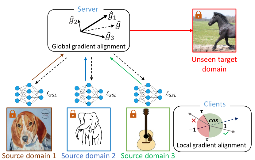
Figure 1: Overview of FedGaLA.

Specifically, the local gradients that are more closely aligned with the average gradient are given greater weight in the aggregation stage. Moreover, we provide a detailed theoretical framework establishing a connection between the alignment of gradients from different clients and the similarity between their data distributions, and thus better domain generalization. Since FedGaLA does not require the sharing of data between clients to perform alignment at either the server or client sides, it effectively preserves data privacy. We verify the performance of our approach using four public datasets, PACS [12], OfficeHome [13], DomainNet [14], and TerraInc [15] and demonstrate strong performance in federated unsupervised domain generalization in comparison to various baselines. Additionally, we conduct different ablation and sensitivity studies to understand the impact of different parameters and the choice of SSL frameworks.

In summary, the main contributions of this study are as follows. (1) To our knowledge, this is the first work to address federated unsupervised domain generalization, introducing a new problem class in this area. (2) We propose a novel technique that considers and aligns gradients at both the local and global levels. Doing so, our solution effectively extracts domain-invariant information in local training and aligns each client’s contributions during the aggregation process, boosting the model’s generalization across various target domains. (3) We conduct extensive experiments and ablations to demonstrate the effectiveness of our proposed method on various benchmarks. We will make our code public upon publication.

2 Related work

Federated learning. Federating learning is a technique of distributed training that enables learning from decentralized clients without the need to transfer raw data to a central server [1, 2]. In the first work in the area of federated learning, FedAVG [1] aggregates the weights of clients via averaging to form the global model. Various federated learning techniques have been since developed for different purposes. FedProx [16] adds a proximal term to the objective to tackle the data heterogeneity problem. FedBuf [17] proposes to use buffered asynchronous aggregation to address scalability and privacy issues. FedALA [18] dynamically aggregates the downloaded global model with the local model on each client, ensuring alignment with the local objective. Moon [5] leverages the similarity between model representations to improve the local training of individual parties through client-level contrastive learning.

Federated domain generalization. This category of problems aims to learn a general model in a privacy-preserving manner that generalizes well to new target domains with distribution shifts [6, 19]. There have been several studies to explore this direction, mainly focusing on learning domain-invariant features [9, 20] or identifying common features across multiple domains [8]. FedDG [6] allows clients to share their data in the frequency space for medical image segmentation. FedSR [9] proposes to learn a simple representation of data to better generalize to target domains through two regularizers, i.e., L2-norm and conditional Mutual Information. FedADG [8] leverages adversarial training to align source domain distributions by matching each distribution with a reference distribution. FedKA [21] learns domain-invariant features by employing feature distribution matching in a universal workspace. CCST [22] aligns various client distributions and mitigates model biases by adapting local models to diverse sample styles via cross-client style transfer. StableFDG [23] uses style and attention-based strategies to address the federated domain generalization problem. Finally, FedDG-GA [24] uses domain divergence and a moment mechanism to enhance generalization through dynamic domain weight adjustment.

Federated unsupervised learning. This category attempts to learn representations from unlabeled data distributed across clients while preserving data privacy [25]. The study by [26] is the first to propose federated unsupervised learning using an encoder-decoder structure. FedU [7] employs a contrastive learning approach with online and target networks to enable each client to independently learn representations from unlabeled data. It also introduces a dynamic aggregation mechanism to update the predictor, either locally or globally. Similarly, FedEMA [27] uses the exponential moving average of the global model to update local ones. FedX [11] proposes to use knowledge distillation to learn representation from local data and refine the central server’s knowledge. FedCA [28] consists of two components: (i) a dictionary module to gather the representations of samples from each client to maintain consistency in the representation space across all clients, and (ii) an alignment module to adjust each client’s representation to match a base model trained on public data.

Federated unsupervised domain generalization. As discussed earlier in Section 1, we define a new problem space not studied previously in the literature, which unifies federated domain generalization and federated unsupervised learning. The key distinction between our new problem definition and standard federated domain generalization is that we assume labels are not available at the client or server levels. On the other hand, our new problem definition differs from standard federated unsupervised learning in that our problem definition assumes domain shifts among clients while existing federated unsupervised methods assume identical data distributions among all clients.

3 Approach

3.1 Problem formulation

To formalize Definition 1, assume $K$ clients, $C_{i}$, in a federated setup, each with access to its own unlabeled data $\mathcal{D}_{i}=\{\textbf{x}_{i}^{(n)}\}_{n=1}^{N_{i}}$. Each dataset consists of $N_{i}$ data points sampled from a distinct data distribution $p(\textbf{x}_{i})$, where $\textbf{x}_{i}$ is a vector of $F$ features, i.e., $\textbf{x}_{i}=[x_{i}^{1},x_{i}^{2},...x_{i}^{F}]^{T}$. The data distributions are assumed to be different among the clients with each distribution $p(\textbf{x}_{i})$ sampled from a family of distributions $\mathcal{P}$. Privacy constraints prevent the transfer of data between clients or to the server $S$. The objective is to learn generalized representations from $\textbf{x}_{i}$ that perform well across unseen distributions $p(\textbf{x}_{t})\sim\mathcal{P}$, where $p(\textbf{x}_{i})\neq p(\textbf{x}_{t})$. This is formulated as minimizing the expected loss over the unseen distributions:

$$\min_{\theta}\mathbb{E}_{p(\textbf{x}_{t})\sim\mathcal{P}}\left[\mathbb{E}_{p(\textbf{x}_{t})}\left[\mathcal{L}(\theta;\textbf{x})\right]\right],$$ (1)

where $\mathcal{L}$ is the unsupervised loss function, and $\theta$ is the set of global model parameters. Each client contributes to this goal by computing a local objective function approximating the expected loss with respect to its own data distribution:

$$\min_{\theta_{i}}\mathbb{E}_{p(\textbf{x}_{i})}\left[l_{i}(\theta_{i};\textbf{x})\right]\approx\frac{1}{N_{i}}\sum^{N_{i}}_{n=1}l(\theta_{i};\textbf{x}_{i}^{(n)}),$$ (2)

where $\theta_{i}$ indicates the local parameters of client $C_{i}$, and $\theta$ is the global aggregation of all local $\theta_{i}$.

3.2 Gradient alignment and domain shift

Under a federated learning framework, privacy constraints prevent clients and servers from accessing each other’s data, including distribution information such as data means and variances. They can, however, observe individual client gradients at the server level and the average aggregated gradient across clients at the client level. We motivate our work on the fact that alignment of gradients may infer characteristics of the client domain distributions, thus facilitating improved model generalization. While empirically the utility of gradients has been demonstrated in the area of domain generalization [29], no theoretical basis has been proposed for this approach under federated constraints. Accordingly, we aim to establish a link between gradient alignment and domain shifts within the proposed problem formulation (Definition 1). Our theoretical findings provide the basis for effective local parameter updates and global model aggregation to address federated unsupervised domain generalization.

Assumption 1.

Let each $\textbf{x}_{i}^{f}$ be a random variable drawn from a Normal distribution $p(\textbf{x}_{i}^{f})\sim\mathcal{P}$ [30]. Within a single domain, following [31, 32], features are assumed to be independent ($Cov(x_{i}^{f_{1}},x_{i}^{f_{2}})=0$). Across different domains, corresponding features of $\textbf{x}_{i}^{f}$ and $\textbf{x}_{j}^{f}$ are bivariate with a covariance of $\sigma_{x_{i}^{f},x_{j}^{f}}$. In line with contemporary practices in deep learning, the features are normalized with $\mu=0$ and $\sigma^{2}=1$ [33, 34, 35]. We also assume that each client is a one-layer encoder with the sigmoid activation function. Following [36], local training is performed using contrastive loss where a random augmentation of a data sample is used as the positive pair and all other samples are utilized as the negative pairs. The random augmentation is performed with the same random Affine transformation ($Ax_{i}+B$) [37] broadcast to all clients. After each epoch, the local models are aggregated in the server and sent back to all clients. The gradient $\textbf{g}_{i}$ of the model is assumed to be differentiable.

Theorem 1 (Gradient Misalignment in Federated Self-supervised Learning Dependent upon Domain Shift).

Given Assumption 1, under the problem proposed in Definition 1, for two distinct domains characterized by random variables $\textbf{x}_{i}$ and $\textbf{x}_{j}$ belonging to two different clients $C_{i}$ and $C_{j}$, an increase in domain shift across the clients results in a decrease in the covariance $\text{Cov}(\emph{$\textbf{g}_{i}$},\emph{$\textbf{g}_{j}$})$ of the corresponding gradients $\textbf{g}_{i}$, $\textbf{g}_{j}$ across $C_{i}$ and $C_{j}$’s respective local models.

Proof of Theorem 1.

Motivated by previous works where the similarity between the representations of different domains under domain shift is measured by Mutual Information [38, 39, 40], we use this concept for modeling the similarity between different domains drawn from a family of distributions. By definition, the Mutual Information between two random variables, $\textbf{x}_{i}$ and $\textbf{x}_{j}$ is

$$I(\textbf{x}_{i};\textbf{x}_{j})=\int\int p(\textbf{x}_{i},\textbf{x}_{j})\log\left(\frac{p(\textbf{x}_{i},\textbf{x}_{j})}{p(\textbf{x}_{i})p(\textbf{x}_{j})}\right)d\textbf{x}_{i}d\textbf{x}_{j}.$$ (3)

Since the domains from which the corresponding random variables are drawn are sets of independent features:

$$p(\textbf{x}_{i})=\prod_{f=1}^{F}p(x_{i}^{f}),\hskip 14.22636ptp(\textbf{x}_{j})=\prod_{f=1}^{F}p(x_{j}^{f}).$$ (4)

Moreover, since each pair of corresponding features ($x_{i}^{f},x_{j}^{f}$) across domains forms a bivariate Normal distribution, we can derive:

$$p(\textbf{x}_{i},\textbf{x}_{j})=\prod_{f=1}^{F}p(x_{i}^{f},x_{j}^{f}).$$ (5)

By substituting Eqs. (4) and (5) into Eq. (3), using the multiplicative property of logarithms and the definition of Mutual Information, we obtain:

$$I(\textbf{x}_{i};\textbf{x}_{j}) =\sum_{f=1}^{F}\int\int p(x_{i}^{f},x_{j}^{f})\log\left(\frac{p(x_{i}^{f},x_{j}^{f})}{p(x_{i}^{f})p(x_{j}^{f})}\right)dx_{i}^{f}dx_{j}^{f}=\sum_{f=1}^{F}I(x_{i}^{f};x_{j}^{f}).$$ (6)

For bivariate Normal distributions $x_{i}$ and $x_{j}$, Mutual Information can be measured by $I(x_{i};x_{j})=-\frac{1}{2}\log(1-\rho^{2})$, where $\rho=\frac{\sigma_{x_{i},x_{j}}}{\sigma_{x_{i}}\sigma_{x_{j}}}$ is the correlation coefficient [41]. Accordingly, Eq. (6) yields:

$$I(\textbf{x}_{i};\textbf{x}_{j})=-\frac{1}{2}\sum_{f=1}^{F}\log(1-(\frac{\sigma_{x_{i}^{f},x_{j}^{f}}}{\sigma_{x_{i}^{f}}\sigma_{x_{j}^{f}}})^{2}).$$ (7)

According to Assumption 1, we have $\sigma_{x_{i}^{f}}=\sigma_{x_{j}^{f}}=1$. Hence, Eq. (7) yields:

$$I(\textbf{x}_{i};\textbf{x}_{j})=-\frac{1}{2}\sum_{f=1}^{F}\log(1-\sigma_{x_{i}^{f},x_{j}^{f}}^{2}).$$ (8)

Since $\sigma_{x_{i}^{f},x_{i}^{f}}=\sigma_{x_{i}^{f}}^{2}$, given identical and standardized domains we have $\sigma_{x_{i}^{f},x_{j}^{f}}=1$. Therefore, we observe from Eq. (8) that as the shift between the domain approaches zero, the Mutual Information approaches infinity. On the other hand, as the two domains shift apart, $\sigma_{x_{i}^{f},x_{j}^{f}}$ approaches zero, and consequently the Mutual information monotonically decreases toward zero. Accordingly, $I(\textbf{x}_{i};\textbf{x}_{j})$ and $\sigma_{x_{i}^{f},x_{i}^{f}}$ are positively and monotonically correlated. To establish the link between the covariance of the features and the variance of the gradient and demonstrate their relationship, the following lemma and claim are introduced.

Lemma 1.

Given Assumption 1, the covariance between the differentiable function g with inputs $\textbf{x}_{i}$ and $\textbf{x}_{j}$ can be estimated as:

$$\text{Cov}(\textbf{g}_{i},\textbf{g}_{j})\approx\sum_{f=1}^{F}\sigma_{x_{i}^{f},x_{j}^{f}}(\frac{\partial\textbf{g}_{i}}{\partial x^{f}_{i}}\bigg{|}_{x^{f}_{i}=\mu^{f}_{i}})(\frac{\partial\textbf{g}_{j}}{\partial x^{f}_{j}}\bigg{|}_{x^{f}_{j}=\mu^{f}_{j}}),$$ (9)

where $\sigma_{x_{i}^{f},x_{j}^{f}}$ is the covariance between the $f^{th}$ feature of $x_{i}$ and $x_{j}$. The proof for this Lemma is provided through the Taylor expansion derived in Appendix A.1.

Claim 1.

For all clients trained under the federated unsupervised domain generalization setup using self-supervised learning described in Assumption 1, and is extra two clients $C_{i}$ and $C_{j}$, for both positive and negative contrastive data pairs, the sign of $(\frac{\partial\textbf{g}_{i}}{\partial x^{f}_{i}}\bigg{|}_{x^{f}_{i}=\mu^{f}_{i}})(\frac{\partial\textbf{g}_{j}}{\partial x^{f}_{j}}\bigg{|}_{x^{f}_{j}=\mu^{f}_{j}})$ is always positive. See proof in Appendix A.2.

According to Eq. (9) introduced in Lemma 1 and Claim 1, we conclude that $\text{Cov}(\textbf{g}_{i},\textbf{g}_{j})$ and $\sigma_{x_{i}^{f},x_{j}^{f}}$ are positively and monotonically correlated. Therefore, $\text{Cov}(\textbf{g}_{i},\textbf{g}_{j})$ and $I(\textbf{x}_{i};\textbf{x}_{j})$ are also positively and monotonically correlated, which completes the proof. ∎

Our theoretical findings may also be applicable to Federated Supervised Domain Generalization, which could form the subject of future research (see Appendix A.5). We further investigate the relationship between the distribution of the domains and their corresponding gradients through the following Corollary.

Corollary 1.

Given the assumptions stated, for two distinct domains characterized by random variables $\textbf{x}_{i}$ and $\textbf{x}_{j}$ from the distribution family $\mathcal{P}$, as $I(\textbf{x}_{i},\textbf{x}_{j})$ decreases, then the variance of the difference of the corresponding gradients, $\text{Var}(\textbf{g}_{i}-\textbf{g}_{j})$, increases. The full proof is presented in Appendix A.3.

3.3 FedGaLA

The analysis above establishes a link between gradient alignment and domain shift, forming the basis for our proposed FedGaLA framework. Figure 1 illustrates an overview of our framework for addressing the newly proposed problem setup (Definition 1). FedGaLA is remotely inspired by prior works that demonstrate improved generalization in centralized (non-federated) learning through gradient alignment [29, 42, 43]. The study in [29] updates the weights if the signs of the gradient components are aligned across all domains. Fish [42] maximizes the inner product between gradients from different domains, while Fishr [43] leverages domain-level gradient variances. However, our framework extends this notion by integrating gradient alignment into the field of unsupervised and federated learning, and assumes, unlike [29, 42, 43], that the distribution of data from different clients is not known. Our core idea includes (i) enabling clients to learn domain-invariant representations at the client level through local gradient alignment, and (ii) adjusting the aggregation weights at the server level using global gradient alignment. At each communication round, clients are initialized with the global model. Subsequently, each client updates its parameters using SSL for $E$ epochs based on the local data through local gradient alignment and sends these updates back to the server. Finally, the server employs the global gradient alignment technique to perform aggregation. This procedure is repeated for $T$ communications rounds to determine the global model. The remaining part of this section provides details on local and global gradient alignment, and the complete framework is outlined in Algorithm 1 (Appendix B).

Local gradient alignment. Our method performs layer-wise local gradient alignment using a reference gradient. This reference is derived from the $l^{\text{th}}$ layer of the global model’s parameter updates between the current and the previous communication round. Suppose $\Theta=\{\theta^{(l)}\}_{l=1}^{L}$ indicates the parameters of the global model, where $\theta^{(l)}$ represents the parameters of the $l^{\text{th}}$ layer. The reference gradient for the $l^{th}$ layer is computed as $\hat{\textbf{g}}_{est}^{(l,t)}=\theta^{(l,t)}-\theta^{(l,t-1)}$, where $\theta^{(l,t)}$ and $\theta^{(l,t-1)}$ are the parameters of the $l^{\text{th}}$ layer of the global model at rounds $t$ and $t-1$, respectively. Then, $\hat{\textbf{g}}_{est}^{(l,t)}$ is locally used to determine whether the gradient of each layer obtained during training (e.g., via SGD) is aligned with the reference. The cosine similarity between the batch gradient and the reference for each layer $l$ at round $t$ is computed as $cos(\phi)^{(l,t)}=\frac{\langle\textbf{g}_{i,k}^{(l,t)},\textbf{g}_{\text{est}}^{(l,t)}\rangle}{\|\textbf{g}_{i,k}^{(l,t)}\|\cdot\|\textbf{g}_{\text{est}}^{(l,t)}\|}$, where $\textbf{g}_{i,k}^{(l,t)}$ is the gradient of $k^{\text{th}}$ batch of the $i^{\text{th}}$ client at layer $l$ and round $t$. Finally, batch gradients whose similarity with $\hat{\textbf{g}}_{est}^{(l,t)}$ are less than a user-defined threshold $\tau$ are discarded during the update process. This prevents clients from learning domain-specific features by disregarding local gradients that are not aligned with the global model.

Global gradient alignment. To aggregate the local (client) models at the server, the locally measured gradients that closely match the average gradient across all clients are assigned greater weights. The process operates as follows. Once the server receives the local models, it first obtains the local update $\hat{\textbf{g}}_{i}^{(t)}=\Theta_{i}^{(t)}-\Theta^{(t-1)}$. Then, the initial global update $\hat{\textbf{g}}^{(t+1)}$ is calculated by averaging all $\hat{\textbf{g}}_{i}^{(t)}$. Subsequently, the weight of each client is computed using $w_{i}=\frac{cos(\hat{\textbf{g}}_{i}^{(t)},\hat{\textbf{g}}^{(t+1)})+1}{2}$, where $w_{i}$ is the weight for the $i^{\text{th}}$ client and $\hat{\textbf{g}}_{i}^{(t)}$ is the gradient of the $i^{\text{th}}$ client at round $t$. This weight reflects the degree of alignment between each client’s update and the global model’s update direction. To ensure these weights are properly normalized using $w_{i}={w_{i}}/{\sum_{k=1}^{K}w_{k}}$. The normalization of weights allows for the proportional contribution of each client’s update.

Finally, the normalized weights are used to perform aggregation. Each client’s model update is scaled by its respective weight, and these weighted updates are then aggregated to compute the weighted average update. The global model at round $t+1$ is updated based on $\hat{\textbf{g}}^{(t+1)}=\frac{1}{K}\sum_{i=1}^{K}w_{i}\hat{\textbf{g}}_{i}^{(t)}$. This aggregation step is repeated three times, refining the weights with each iteration. This ensures the global model update is significantly influenced by clients whose updates align closely with the global learning objective. After completing the aggregation process, the global model is further updated based on $\Theta^{(t+1)}\leftarrow\Theta^{(t)}+\hat{\textbf{g}}^{(t+1)}$.

4 Experiment setup

Datasets. To evaluate the effectiveness of our proposed method, we conduct experiments across four commonly used benchmarks for domain generalization. They include: PACS [44], which consists of 9,991 images from four domains: ‘Photo’, ‘Art-painting’, ‘Cartoon’, and ‘Sketch’, across seven classes; Office-Home [13], which consists of 15,588 images from four domains: ‘Art’, ‘Clipart’, ‘Product’, and ‘Real-world’, across 65 classes; TerraInc [15], which includes 24,788 images from four domains ‘Location 38’, ‘Location 43’, ‘Location 46’, and ‘Location 100’, across nine classes; DomainNet [14], which consists of 569,010 images in six domains: ‘Clipart’, ‘Infograph’, ‘Painting’, ‘Quickdraw’, ‘Real’, and ‘Sketch’, covering 345 classes. We follow the same protocol as [45] for this dataset (see details in Appendix D.1).

Evaluation. We use the leave-one-domain-out setting used in prior works [28, 45, 46]. This involves selecting one domain as the target, training the model on the rest of the domains, and then testing the model’s performance on the selected target domain. Linear evaluation, a common feature evaluation approach, is utilized to evaluate the quality of learned representations [47, 48, 49]. For linear evaluation, following [26, 27], we utilize 10% and 30% of the target data to train the linear classifier, and evaluate the remaining 90% and 70% of the data, respectively.

Table 1: Results of linear eval. on PACS, DomainNet, Office-Home, and TerraInc datasets.

Model Labeled PACS DomainNet ratio P A C S Ave. C I Q Ave. FedEMA 10% 50.0(0.7) 29.5(1.9) 42.4(2.3) 45.6(0.16) 41.9 38.6(1.1) 13.7(0.5) 45.5(1.6) 32.4 FedBYOL 52.1(1.1) 31.8(1.1) 45.4(2.2) 47.4(1.9) 44.2 38.1(0.5) 14.1(0.4) 53.6(2.9) 31.8 FedMoCo 58.5(2.2) 35.7(9.6) 37.7(12.9) 36.6(8.2) 42.1 30.5(0.6) 10.9(2.1) 46.4(0.8) 27.2 FedSimSiam 46.2(1.1) 28.6(1.0) 46.7(0.6) 37.6(1.3) 39.8 44.8(1.5) 12.2(0.3) 40.3(2.4) 36.9 FedSimCLR 64.2(1.2) 41.9(1.5) 58.4(1.3) 70.1(1.2) 58.6 45.2(0.4) 13.7(0.3) 59.7(0.7) 39.5 FedGaLA (ours) 64.7(1.9) 44.2(1.2) 60.5(2.2) 70.5(1.3) 60.0 47.6(0.9) 14.2(0.5) 61.4(0.3) 41.1 FedEMA 30% 33.9(2.8) 48.3(2.4) 53.5(0.3) 45.3(2.3) 45.2 43.5(0.8) 20.0(1.5) 49.0(2.8) 37.5 FedBYOL 55.1(1.2) 35.3(1.5) 48.3(1.5) 48.9(0.5) 46.9 44.6(1.2) 20.5(1.1) 50.4(0.9) 38.5 FedSimSiam 58.5(2.2) 35.7(9.6) 37.7(12.9) 36.6(8.2) 42.1 35.7(1.1) 14.9(3.9) 44.6(3.5) 31.8 FedMoCo 47.3(1.6) 30.2(3.4) 47.4(0.7) 34.4(1.7) 39.9 51.5(1.8) 18.2(0.1) 59.9(3.6) 43.2 FedSimCLR 69.8(1.1) 46.4(2.1) 63.9(1.6) 73.4(3.0) 63.3 51.7(1.0) 16.3(0.2) 66.5(0.9) 44.8 FedGaLA (ours) 71.1(2.0) 46.8(2.1) 65.7(1.6) 74.5(1.1) 64.6 52.4(0.7) 16.2(0.6) 68.8(0.6) 45.8

Model	Labeled	Office-Home					TerraInc
	ratio	A	C	P	R	Ave.	L38	L43	L46	L100	Ave.
FedEMA	10%	20.8(0.9)	6.7(0.5)	12.5(0.4)	14.1(0.8)	13.5	62.1(0.4)	43.5(3.0)	43.4(0.4)	63.9(0.7)	53.2
FedBYOL		7.4(0.3)	12.9(0.5)	20.9(1.1)	13.8(0.1)	13.8	63.4(0.2)	43.3(0.5)	44.3(0.3)	66.3(2.4)	54.3
FedSimSiam		8.5(0.5)	19.8(0.8)	28.2(0.8)	16.2(0.6)	18.9	54.0(6.8)	36.0(1.5)	40.9(3.7)	60.8(1.6)	47.9
FedMoCo		10.8(0.4)	9.4(0.3)	12.4(0.9)	10.1(0.7)	10.7	50.0(2.4)	33.8(0.3)	29.7(2.3)	60.2(0.1)	45.7
FedSimCLR		8.9(0.4)	24.3(0.3)	35.2(1.2)	20.0(0.2)	22.0	62.8(0.2)	45.8(1.1)	42.9(1.8)	68.8(0.3)	55.1
FedGaLA (ours)		8.9(0.4)	25.3(0.6)	36.6(0.3)	21.2(0.5)	23.0	63.6(0.1)	47.6(1.4)	43.9(2.9)	71.7(0.9)	56.7
FedEMA	30%	10.0(0.3)	17.3(0.7)	28.2(1.1)	17.8(0.3)	18.2	62.7(0.6)	47.1(0.3)	46.1(0.4)	67.6(2.0)	55.9
FedBYOL		10.4(0.3)	17.4(1.2)	29.4(1.3)	17.6(0.6)	18.7	63.6(0.9)	46.7(1.3)	46.1(0.2)	68.8(2.5)	56.3
FedSimSiam		12.7(1.1)	24.1(1.9)	36.5(0.7)	21.6(1.1)	23.7	56.8(4.6)	35.7(2.0)	38.9(4.6)	61.4(1.4)	48.2
FedMoCo		15.2(0.6)	11.2(0.9)	15.8(0.7)	11.5(1.6)	13.4	60.7(0.1)	28.3(3.3)	31.7(2.3)	60.0(0.6)	45.2
FedSimCLR		13.6(1.3)	35.3(0.7)	47.6(0.9)	26.6(1.0)	30.7	65.8(0.3)	54.5(1.2)	49.0(0.4)	71.0(1.6)	60.1
FedGaLA (ours)		13.6(0.6)	35.1(0.2)	48.0(1.3)	27.0(0.7)	30.9	66.2(0.5)	52.4(1.7)	51.7(0.8)	74.6(1.3)	61.3

Baselines. To evaluate our method, we take a two-pronged approach: (1) We adapt several popular SSL approaches to the federated domain generalization task, denoting them as FedSimCLR, FedMoCo, FedBYOL, and FedSimSiam. To do so, we first train each client locally using the respective SSL method. Next, we aggregate the trained encoders at the server using FedAVG [1]. For BYOL and SimSiam, we follow the procedure in [7] and apply FedAVG on the online encoder and projector. We also adapt FedEMA [27], a notable federated SSL method originally developed to address the non-IID problem, as another method for performance comparison. FedEMA integrates BYOL as an SSL technique into its structure. Additional details regarding SSL baselines are presented in Appendix C. It is important to note that we avoid direct comparisons with FedDG [6], FedSR [9], FedADG [8], and FedDG-GA [24] since unlike our method, they employ the label information in their solutions. (2) Given the absence of prior research specifically addressing the problem of federated unsupervised domain generalization, we also compare FedGaLA to established centralized unsupervised domain generalization methods on the PACS and DomainNet datasets. We could not identify unsupervised domain generalization methods for Office-Home and TerraInc datasets. This comparison includes the following solutions: SimCLR [36], MoCo [50], BYOL [51], AdCo [52], and DARLING [45]. It is important to note that these methods are implemented in a non-federated environment and do not incorporate any data privacy constraints. All the results for these models are reported from [45].

Implementation details. We use SimCLR as the SSL module in FedGaLA due to its performance on domain generalization problems as previously shown [45]. Following[45], ResNet-18 [53] is employed as the encoder network architecture for all experiments, which we train from scratch. We present details regarding data augmentations, projector architecture, and encoder hyperparameters in Appendix D. Following [47, 48], we first learn a representation by FedGaLA and the baseline models for 100 communication rounds with 7 local epochs. Next, we freeze the backbone model and train a liner classier for 100 epochs to perform prediction on the target domain. Appendix D presents all the hyperparameters used for FedGaLA. For FedEMA, we use the hyperparameters reported in [27]. All experiments were implemented using PyTorch and trained on 8 NVIDIA GeForce RTX 3090 GPUs.

5 Results

Performance. We report the accuracy rates of FedGaLA and baseline models on the four datasets. As shown in Table 1, FedGaLA consistently outperforms all baselines across all four datasets, with the exception of ‘Art-painting’ domain in Office-Home, for the 10% data regime. When 30% of the data are used, our method still generally outperforms the baseline models, although for some of the domains, the baseline solutions produce slightly better results. This observation is expected given that with the introduction of more domain-specific training data, the need for domain generalization declines, and thus, methods that are not explicitly designed for domain generalization can produce competitive results. Across the four datasets, we observe that among the baseline models, FedSimCLR achieves better results compared to FedSimSiam, FedBYOL, and FedMoCo. This finding is consistent with [45] where it was demonstrated that SimCLR provides a better foundation for domain generalization versus other SSL methods, albeit in a non-federated setup. Table 2 compares the performance of FedGaLA with non-federated (centralized) methods for PACS and DomainNet datasets. As shown in this table, FedGaLA outperforms these methods by large margins. This is an expected observation as prior works have shown that federation can boost domain generalization [9, 54].

Table 2: Comparison of linear eval. (10%) results with non-federated (centralized) domain generalization methods on PACS and DomainNet datasets.

Model PACS DomainNet P A C S Ave. C I Q Ave. BYOL 27.0 25.9 21.0 19.7 23.4 14.6 8.7 5.9 9.7 MoCo 44.2 25.9 33.5 25.0 32.1 32.5 18.5 8.1 19.7 SimCLR 54.7 37.7 46.00 28.3 41.6 37.1 19.9 12.3 23.1 AdCo 46.5 30.2 31.5 22.9 32.8 32.3 17.9 11.6 20.6 DARLING 53.4 39.9 46.4 30.2 42.5 35.2 20.9 15.7 23.9 FedGaLA (ours) 64.7(1.9) 44.2(1.2) 60.5(2.2) 70.5(1.3) 60.0 47.6(0.9) 14.2(0.5) 61.4(0.3) 41.1

Table 3: Ablation study on PACS (GA: global alignment; LA: local alignment).

Models	P	A	C	S	Ave.
FedGaLA	64.7(1.9)	44.2(1.2)	60.5(2.2)	70.5(1.3)	60.0
w/o GA	64.7(0.4)	42.6(1.2)	58.1(0.6)	69.9(1.1)	58.8
w/o LA	63.7(1.5)	41.6(1.4)	59.8(1.5)	68.9(1.1)	58.5
w/o GA & LA	64.2(1.2)	41.9(1.5)	58.4(1.3)	70.1(1.2)	58.6

Ablation studies. Here we examine the effectiveness of the local and global gradient alignment components individually on the final performance of FedGaLA. To this end, we systematically remove each of these components. As shown in Table 3, each component plays an important role in the overall performance. It is noteworthy to mention that FedGaLA essentially becomes the FedSimCLR baseline by removing both global and local alignments.

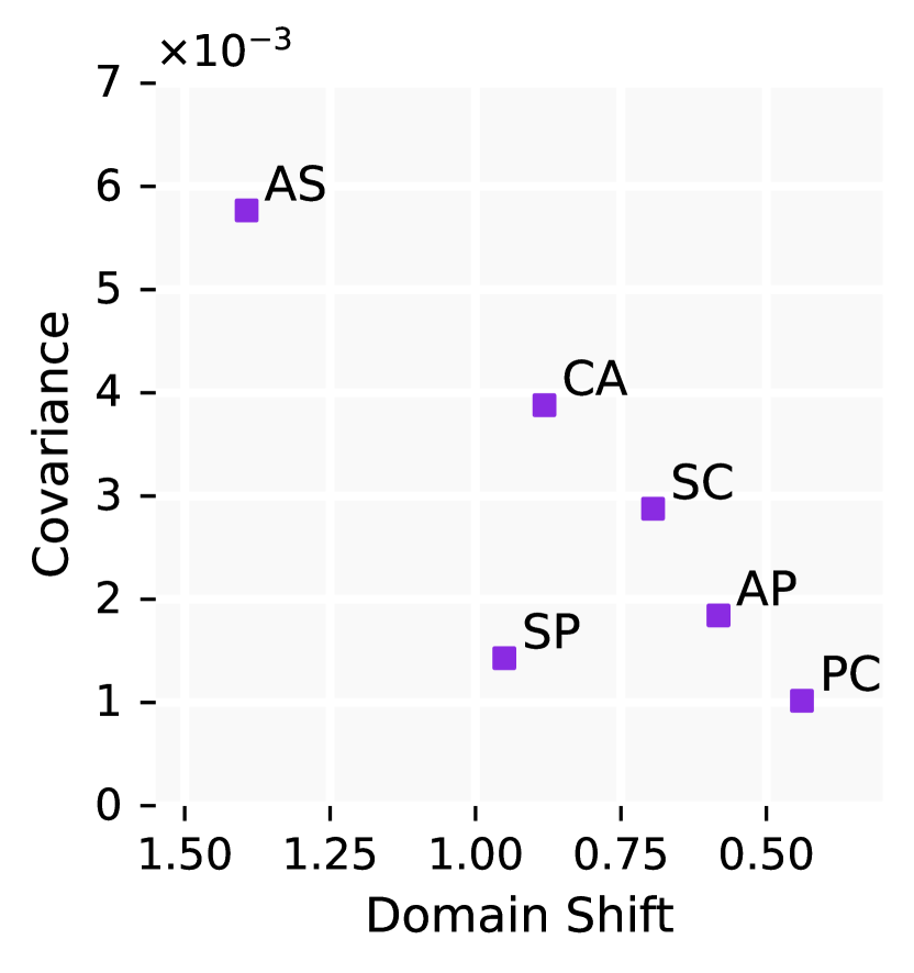
Figure 2: Covariance against domain shift for P, A, C, and S.

Gradient misalignment due to domain shift. In Figure 2 we illustrate the amount of measured covariance for different domains in PACS versus the amount of domain shift between each pair measured through Mutual Information. We observe that, except for a single outlier, the trend follows our prediction based on Theorem 1.

Analysis. All experiments below are performed on the PACS dataset using the domain ‘Photo’ unless otherwise mentioned. Additional analyses are also presented in Appendix E.

Ratio of labeled data. Figure 3(a) presents the results when evaluated with different ratios of labeled data, ranging from 10% to 60%. As can be seen, the accuracy increases significantly from 64% to 72% when the labeled ratio rises from 10% to 30%, followed by a steady climb to 74% as the labeled ratios increase to 60%. Overall, when more labeled data are used to train the linear classifier, the final performance expectedly improves.

Ratio of discarded local gradients. Figure 3(b) demonstrates the ratio of local gradients discarded due to local gradient alignment during training versus communication rounds. For this experiment, the local models are trained for 1 epoch at each communication round. As observed, the ratio of discarded local gradients decreases from approximately 68% in the early communication rounds to 37% by round 100. This trend indicates that as the number of communication rounds increases, the local gradient directions become more aligned with the global model, suggesting that with increasing the number of communications, local models learn more domain-invariant features.

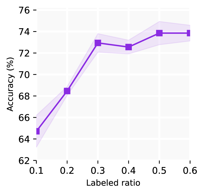
(a)

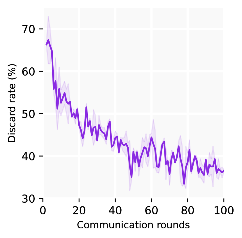
(b)

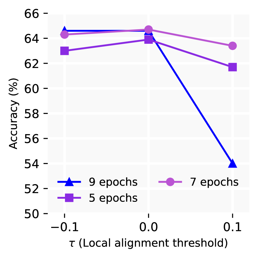
(c)

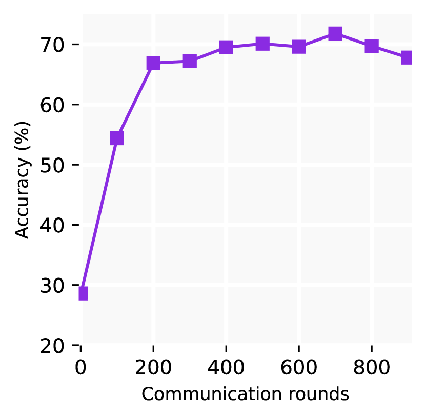
(d)

Figure 3: Impact of different labeled data ratios on linear evaluation (a) and average ratio of discarded local gradients over 100 communication rounds for $\tau=0$ and $E=1$ (b). The impact of the local threshold for different numbers of local epochs (c) and communication rounds (d) on performance.

Local threshold vs. the number of local epochs. In Figure 3(c) we study the impact of the threshold for the similarity between gradients and the reference ($\tau$) and the number of local epochs $E$ on performance. In this experiment, we use three different values for $\tau$: $-$0.1, 0, and 0.1, and three different values for $E$: 5, 7 or 9 (local epochs per communication round). We observe that our method produces the best results when $\tau=0$, i.e., when we keep all gradients with positive cosine similarity with the reference. Expectedly, even discarding gradients with small amounts of alignment ($\tau=0.1$) degrades the results, while keeping gradients that are not aligned with the reference ($\tau=-0.1$) also hurts performance. Moreover, we see that setting $E=7$ yields the best performance as increasing the number of epochs beyond 7 does not have a positive impact, and only increases computational time.

Communication rounds. We investigate the effect of the communication rounds $T$ on the model’s performance. Following [7, 27] we set $E=1$ and vary the number of communication rounds $T$ from 100 to 900. We observe from Figure 3(d) that performance improves significantly from 1 to 200 communication rounds, with this trend slowing down from 200 to 900.

Effects of regularizers on FedGaLA. Prior works have demonstrated that adding regularizers can indeed improved generalization across domains or non-IID data [16, 9]. To this end, we test the impact of regularizers on FedGaLA by applying two types of regularizers based on L2 norm [16] and FedProx [9]. Please refer to Appendix D.5 for more details regarding these two techniques. The results in Table 4 demonstrate that FedGaLA is highly compatible with regularizers and that the addition of such approaches can further boost the performance of our method.

Table 4: The effect of regularizers on the performance of FedGaLA across PACS, DomainNet, Office-Home, and TerraInc datasets.

Model PACS DomainNet P A C S Ave. C I Q Ave. FedGaLA+L2 ($\lambda=0.001$) 64.8(0.5) 42.8(1.1) 58.7(1.6) 67.3(0.6) 58.4 46.3(0.8) 16.4(0.9) 62.8(0.2) 41.6 FedGaLa+L2 ($\lambda=0.01$) 66.5(0.9) 43.4(0.9) 56.9(2.7) 65.2(0.6) 57.9 38.9(1.2) 14.6(0.7) 52.5(0.8) 35.3 FedGaLA+FedProx ($\mu=0.001$) 62.1(0.2) 41.4(0.7) 58.9(3.1) 68.8(0.1) 57.8 44.6(0.2) 13.4(1.0) 60.9(1.1) 39.6 FedGaLA+FedProx ($\mu=0.01$) 63.1(0.2) 41.6(1.2) 58.5(2.0) 68.9(1.9) 58.0 44.7(1.2) 13.2(0.4) 61.7(0.4) 39.9 FedGaLA (ours) 64.7(1.9) 44.2(1.2) 60.5(2.2) 70.5(1.3) 60.0 47.6(0.9) 14.2(0.5) 61.4(0.3) 41.1

Model Office-Home TerraInc A C P R Ave. L38 L43 L46 L100 Ave. FedGaLA+L2 ($\lambda=0.001$) 11.8(0.4) 23.9(0.5) 37.1(0.4) 21.9(0.7) 23.6 61.6(0.9) 45.8(0.6) 46.6(0.7) 70.8(0.7) 56.2 FedGaLa+L2 ($\lambda=0.01$) 11.8(0.2) 21.2(0.1) 34.5(0.3) 22.1(0.2) 22.4 61.5(0.7) 38.1(2.9) 44.9(0.1) 57.8(3.3) 50.6 FedGaLA+FedProx ($\mu=0.001$) 10.2(0.4) 24.2(0.4) 36.4(1.1) 19.7(0.32) 22.6 63.8(0.7) 49.3(1.5) 47.2(0.1) 71.5(0.9) 57.9 FedGaLA+FedProx ($\mu=0.01$) 9.2(0.3) 23.6(0.7) 37.1(0.6) 20.4(0.4) 22.6 63.2(1.1) 47.8(2.1) 44.8(0.4) 71.4(0.8) 56.0 FedGaLA (ours) 8.9(0.4) 25.3(0.6) 36.6(0.3) 21.2(0.5) 23.0 63.6(0.1) 47.6(1.4) 43.9(2.9) 71.7(0.9) 56.7

FedGaLA with other SSL techniques. We examine the effectiveness of FedGaLA using other SSL frameworks (MoCo, BYOL, and SimCLR), on the PACS dataset and present the results in Appendix E. Our findings suggest that FedGaLA can improve the performance of various SSL baselines for federated unsupervised domain generalization.

6 Conclusion

In this work, we first introduced a new problem category, federated unsupervised domain generalization, and subsequently proposed FedGaLA to tackle it. Building the relationship between gradient alignment and domain shift, FedGaLA comprises two alignment strategies at the global and local levels designed to address the problem of domain generalization in an unsupervised and federated setup. We assessed the performance of FedGaLA through extensive experiments where our approach outperformed various baseline models. Detailed ablation studies and sensitivity analyses were also conducted to provide more insights into different aspects of our solution.
Limitations. Given the emphasis of federated learning on privacy and safety, the robustness of FedGaLA against adversarial attacks, particularly those targeting the gradient exchange process, remains an unexplored area, which can be an interesting future research direction.

Appendix A Proofs

A.1 Proof of Lemma 1

Proof.

The covariance of $\textbf{g}_{i}$ and $\textbf{g}_{j}$, by definition, is:

$$\text{Cov}(\textbf{g}_{i},\textbf{g}_{j})=\mathbb{E}\{(\textbf{g}_{i}-\mathbb{E}\{\textbf{g}_{i}\})(\textbf{g}_{j}-\mathbb{E}\{\textbf{g}_{j}\})\}.$$ (1)

First, we calculate $\mathbb{E}{\textbf{g}_{i}}$. Given g is differentiable, as per the Assumption 1, we can estimate it using the first-degree Taylor expansion theorem around $\mu$:

$$g(x)\approx g(\mu)+\sum_{f=1}^{F}(x^{f}-\mu^{f})\left(\frac{\partial g}{\partial x^{f}}\bigg{|}_{x^{f}=\mu^{f}}\right).$$ (2)

We can use this equation to estimate $\mathbb{E}{\textbf{g}}$ as follows:

$$\mathbb{E}{\textbf{g}}=\mathbb{E}{g(\mu)+\sum_{f=1}^{F}(x^{f}-\mu^{f})\left(\frac{\partial g}{\partial x^{f}}\bigg{|}_{x^{f}=\mu^{f}}\right)}.$$ (3)

Note that $g(\mu)$ is constant, therefore $\mathbb{E}{g(\mu)}=g(\mu)$. Moreover, since we assume that the distribution of the features is normal, we can conclude:

$$\mathbb{E}{\sum_{f=1}^{F}(x^{f}-\mu^{f})\left(\frac{\partial g}{\partial x^{f}}\bigg{|}_{x^{f}=\mu^{f}}\right)}=0.$$ (4)

Since $\mathbb{E}{x^{f}-\mu^{f}}=0$ for $x^{f}\sim\mathcal{N}$, $\mathbb{E}{g}=g(\mu)$. By replacing $g_{i}$ and $g_{j}$ with their Taylor expansion we derive:

$$\text{Cov}(\textbf{g}_{i},\textbf{g}_{j})= \mathbb{E}\left[\left(\sum_{f=1}^{F}(x_{i}^{f}-\mu_{i}^{f})\left(\frac{\partial g}{\partial x_{i}^{f}}\bigg{|}_{x_{i}^{f}=\mu_{i}^{f}}\right)\right)\right.\left.\left(\sum_{f=1}^{F}(x_{j}^{f}-\mu_{j}^{f})\left(\frac{\partial g}{\partial x_{j}^{f}}\bigg{|}_{x_{j}^{f}=\mu_{j}^{f}}\right)\right)\right].$$ (5)

Hence:

$$\text{Cov}(\textbf{g}_{i},\textbf{g}_{j})=\mathbb{E}\left[\sum_{f=1}^{F}\sum_{e=1}^{F}(x_{i}^{f}-\mu_{i}^{f})(x_{j}^{e}-\mu_{j}^{e})\left(\frac{\partial g}{\partial x_{i}^{f}}\bigg{|}_{x_{i}^{f}=\mu_{i}^{f}}\right)\right.\left.\left(\frac{\partial g}{\partial x_{j}^{e}}\bigg{|}_{x_{j}^{e}=\mu_{j}^{e}}\right)\right].$$ (6)

Given $\text{Cov}(x^{f}_{i},x^{e}_{j})=\mathbb{E}{(x^{f}_{i}-\mu^{f}_{i})(x^{e}_{j}-\mu^{e}_{j})}=\sigma_{x^{f}_{i},x^{f}_{j}}$, we derive:

$$\text{Cov}(\textbf{g}_{i},\textbf{g}_{j})=\sum_{f=1}^{F}\sum_{e=1}^{F}\sigma_{x^{f}_{i},x^{f}_{j}}\left(\frac{\partial g}{\partial x_{i}^{f}}\bigg{|}_{x_{i}^{f}=\mu_{i}^{f}}\right)\left(\frac{\partial g}{\partial x_{j}^{e}}\bigg{|}_{x_{j}^{e}=\mu_{j}^{e}}\right).$$ (7)

As the features are assumed to be independent, $\text{Cov}(x^{f}_{i},x^{e}_{j})=0$ when $f\neq e$, we have:

$$\text{Cov}(\textbf{g}_{i},\textbf{g}_{j})=\sum_{f=1}^{F}\sigma_{x^{f}_{i},x^{f}_{j}}\left(\frac{\partial g}{\partial x_{i}^{f}}\bigg{|}_{x_{i}^{f}=\mu_{i}^{f}}\right)\left(\frac{\partial g}{\partial x_{j}^{f}}\bigg{|}_{x_{j}^{f}=\mu_{j}^{f}}\right).$$ (8)

which completes the proof. ∎

A.2 Proof of Claim 1

Proof.

Following Assumption 1, the model is defined as $\hat{y}=\sigma(Wx_{1}-Wx_{2})$ and the loss is formulated as:

$$l(y,\hat{y})=-y\log(\hat{y})-(1-y)\log(1-\hat{y}),$$ (9)

where $y=1$ for positive pairs and $y=0$ for the negative pairs. Consequently, the gradient of the loss w.r.t. $W$ is

$$g=\left\{\begin{array}[]{ll}(\sigma(Wx_{1}-Wx_{2})-1)(x_{1}-x_{2})&\text{if }y=1\text{ (Positive pairs)}\\ \sigma(Wx_{1}-Wx_{2})(x_{1}-x_{2})&\text{if }y=0\text{ (Negative pairs)}\end{array}\right.$$ (10)

We first focus on the positive pairs. In the contrastive loss, an augmentation of the same sample is usually used as the positive sample. Following Assumption 1, the augmented sample is formulated as ${x}_{2}=Ax_{1}+B$. Hence, the gradient of the positive pair is derived as:

$$g^{+}=(\sigma(Wx_{1}-WAx_{1}-WB)-1)(x_{1}-Ax_{1}-B)$$ (11)

Subsequently, the derivative of $g^{+}$ with respect to $x_{1}$ at $x_{1}=\mu_{1}$ is expressed as:

$$\frac{\partial{g^{+}}}{\partial x_{1}}\bigg{|}_{x_{1}=\mu_{1}} =\sigma(W\mu_{1}-WA\mu-WB)(1-\sigma(W\mu_{1}-WA\mu_{1}-WB))(\mu_{1}-A\mu-B)$$

$$+\sigma(W\mu_{1}-WA\mu_{1}-WB)(1-A).$$ (12)

Recall Assumption 1 stating that the data is normalized, hence, $\mu_{1}=0$. Therefore:

$$\frac{\partial{g^{+}}}{\partial x_{1}}\bigg{|}_{x_{1}=\mu_{1}}=\sigma(-WB)(1-\sigma(-WB))(-B)+\sigma(-WB)(1-A).$$ (13)

As a result, we can conclude that for all positive pairs, $\frac{\partial{g^{+}}}{\partial x_{i}}\bigg{|}_{x_{i}=\mu_{i}}$ only depends on the augmentation and the network weights. According to Assumption 1, the weights of clients are the same and equal to the global model at each communication round. Moreover, since the same random augmentations are broadcasted to all the clients, $A$ and $B$ will be the same at each step across all the local models. Hence, for all $x_{i}$, $\text{sign}(\frac{\partial{g}_{i}}{\partial x^{f}_{i}}\big{|}_{x^{f}_{i}=\mu^{f}_{i}})=\text{sign}(\frac{\partial{g}_{j}}{\partial x^{f}_{j}}\big{|}_{x^{f}_{j}=\mu^{f}_{j}}).$

Considering the negative pairs, from Eq. (10), we have:

$$g^{-}=\sigma(Wx_{1}-Wx_{2})(x_{1}-x_{2}).$$ (14)

The derivative of $g^{-}$ w.r.t. $x_{1}$ at $x_{1}=\mu_{1}$ is derived as:

$$\frac{\partial{g^{-}}}{\partial x_{1}}\bigg{|}_{x_{1}=\mu_{1}} =\sigma(W\mu_{1}-Wx_{2})(1-\sigma(W\mu_{1}-Wx_{2}))(\mu_{1}-Ax_{2})$$

$$+\sigma(W\mu_{1}-Wx_{2})(1-x_{2}).$$ (15)

Based on the stated assumption $\mu_{1}=0$, therefore:

$$\frac{\partial{g^{-}}}{\partial x_{1}}\bigg{|}_{x_{1}=\mu_{1}}=\sigma(-Wx_{2})(1-\sigma(-Wx_{2}))(-Ax_{2})+\sigma(-Wx_{2})(1-x_{2}).$$ (16)

The $\sigma$ function is estimated using Taylor expansion around zero (since the data is normalized to $\mu=0$), as:

$$\sigma(x)\simeq\frac{1}{2}+\sum_{n=0}^{\infty}\frac{(-1)^{n}(2^{2n+1}-1)B_{2n+2}}{(2n+2)!}x^{2n+1},$$ (17)

where $B_{n}$ are Bernoulli numbers. By replacing Eq. (17) in Eq. (16):

$$\frac{\partial g^{-}}{\partial x_{1}}\bigg{|}_{x_{1}=\mu_{1}} \simeq\left(\frac{1}{2}+\sum_{n=0}^{\infty}\frac{(-1)^{n+1}(2^{2n+1}-1)B_{2n+2}}{(2n+2)!}(Wx_{2})^{2n+1}\right)$$

$$\quad\times\left(\frac{1}{2}-\sum_{n=0}^{\infty}\frac{(-1)^{n+1}(2^{2n+1}-1)B_{2n+2}}{(2n+2)!}(Wx_{2})^{2n+1}\right)(-Ax_{2})$$

$$\quad+\left(\frac{1}{2}+\sum_{n=0}^{\infty}\frac{(-1)^{n+1}(2^{2n+1}-1)B_{2n+2}}{(2n+2)!}(Wx_{2})^{2n+1}\right)(1-x_{2}).$$ (18)

Since the coeffiencts are only consist of $n$, $B_{n}$ and $W$, we can simplify as:

$$\frac{\partial{g^{-}}}{\partial x_{1}}\bigg{|}_{x_{1}=\mu_{1}}\approx\sum_{n=0}^{\infty}\zeta(W,n)x_{2}^{n}$$ (19)

Since the gradient is a linear operation, the gradient of the sum equals the sum of gradients. According to Assumption A1, we update the model with the loss of the entire dataset as the negative samples. Hence:

$$\frac{\partial{g^{-}}}{\partial x_{1}}\bigg{|}_{x_{1}=\mu_{1}}=\sum_{i=2}^{N}\sum_{n=0}^{\infty}\zeta(W,n)x_{i}^{n}.$$ (20)

By substituting the sums, we derive:

$$\frac{\partial{g^{-}}}{\partial x_{1}}\bigg{|}_{x_{1}=\mu_{1}}=\sum_{n=0}^{\infty}\sum_{i=2}^{N}\zeta(W,n)x_{i}^{n}.$$ (21)

Since the distribution of data is assumed to be normal, these sums can be estimated using the expected value of $\mathbb{E}(\sum_{i=1}^{N}x_{i}^{n})=N\mathbb{E}(x^{n})$. Since $x$ belongs to a normal distribution with $\mu=0$ and $\sigma=1$, the sum can be estimated as:

$$\sum_{i=1}^{N}x^{n}\simeq\left\{\begin{array}[]{cll}(n-1)!!&n=2k&\text{ (Even powers)}\\ 0&n=2k+1&\text{ (Odd powers)}\end{array}\right.$$ (22)

By applying this estimate to Eq. ( 20), we derive:

$$\frac{\partial{g^{-}}}{\partial x_{1}}\bigg{|}_{x_{1}=\mu_{1}}=\sum_{k=0}^{\infty}\sum_{i=2}^{N}\zeta(W,n)(n-1)!!$$ (23)

Consequently, we can conclude that for all negative pairs, the gradient derivative $\frac{\partial{g^{-}}}{\partial x_{i}}\bigg{|}_{x_{i}=\mu_{i}}$ only depends on the network weights. Hence, $\text{sign}(\frac{\partial{g}_{i}}{\partial x^{f}_{i}}\big{|}_{x^{f}_{i}=\mu^{f}_{i}})=\text{sign}(\frac{\partial{g}_{j}}{\partial x^{f}_{j}}\big{|}_{x^{f}_{j}=\mu^{f}_{j}}).$

∎

A.3 Proof of Corollary 1

Proof.

The variance of $\textbf{g}_{i}$ and $\textbf{g}_{j}$ is:

$$\text{Var}(\textbf{g}_{i}-\textbf{g}_{j})=\text{Var}(\textbf{g}_{i})+\text{Var}(\textbf{g}_{j})-2\text{Cov}(\textbf{g}_{i},\textbf{g}_{j}).$$ (24)

For deriving $\text{Var}(\textbf{g}_{i})$ and $\text{Var}(\textbf{g}_{j})$, we first introduce Lemma A1.

Lemma A1.

Given the assumptions stated, the variance of a differentiable function g can be estimated as:

$$\text{Var}(\textbf{g})=\sum_{f=1}^{F}(\sigma^{f})^{2}(\frac{\partial{g}}{\partial x^{f}}\bigg{|}_{x^{f}=\mu^{f}})^{2},$$ (25)

where $x^{f}$ is the $f^{th}$ feature of x, $\sigma^{f}$ is its standard deviation, and $\mu^{f}$ is its mean. The full proof of this lemma is presented in Appendix A.4.

By derive $\text{Var}(\textbf{g}_{i})$ and $\text{Var}(\textbf{g}_{j})$ using Lemma 2 and $\text{Cov}(\textbf{g}_{i},\textbf{g}_{j})$ from Lemma 1, we derive:

$$\text{Var}(\textbf{g}_{i}-\textbf{g}_{j})=\sum_{f=1}^{F}(\sigma^{f}_{i})^{2}(\frac{\partial{g}_{i}}{\partial x^{f}_{i}}\bigg{|}_{x^{f}_{i}=\mu^{f}_{i}})^{2}+(\sigma^{f}_{j})^{2}(\frac{\partial{g}_{j}}{\partial x^{f}_{j}}\bigg{|}_{x^{f}_{j}=\mu^{f}_{j}})^{2}-2\sigma_{x_{i}^{f},x_{j}^{f}}(\frac{\partial{g}_{i}}{\partial x^{f}_{i}}\bigg{|}_{x^{f}_{i}=\mu^{f}_{i}})(\frac{\partial{g}_{j}}{\partial x^{f}_{j}}\bigg{|}_{x^{f}_{j}=\mu^{f}_{j}}).$$ (26)

If we assume two domains that have the same distribution but different covariances with $\textbf{g}_{i}$ denoted by $\textbf{g}_{j1}$ and $\textbf{g}_{j2}$, then:

$$\text{Var}(\textbf{g}_{i}-\textbf{g}_{j1})-\text{Var}(\textbf{g}_{i}-\textbf{g}_{j2})=\sum_{f=1}^{F}\alpha_{f}(\sigma^{f}_{ij1}-\sigma^{f}_{ij2}),$$ (27)

where $\alpha_{f}=2(\frac{\partial{g}_{i}}{\partial x^{f}_{i}}\bigg{|}_{x^{f}_{i}=\mu^{f}_{i}})(\frac{\partial{g}_{j}}{\partial x^{f}_{j}}\bigg{|}_{x^{f}_{j}=\mu^{f}_{j}})$ which is always positive (According to Claims A1 and 1). ∎

This conclusion highlights our finding in Theorem 1 regarding the relationship between the distribution of different domains and their corresponding gradients.

A.4 Proof of Lemma A1

Proof.

The variance of g, by definition, is:

$$\text{Var}(\textbf{g})=\mathbb{E}{(\textbf{g}-\mathbb{E}{\textbf{g}})^{2}}.$$ (28)

From the proof of Lemma 2, we know that $\mathbb{E}{g}=g(\mu)$. By expanding $g$ around $\mu$ we derive:

$$\text{Var}(\textbf{g})=\mathbb{E}\left[\left(\sum_{f=1}^{F}(x^{f}-\mu^{f})\left(\frac{\partial g}{\partial x^{f}}\bigg{|}_{x^{f}=\mu^{f}}\right)\right)^{2}\right].$$ (29)

The squared term can be expanded as:

$$\text{Var}(\textbf{g})=\mathbb{E}\left[\sum_{f=1}^{F}\sum_{e=1}^{F}(x^{f}-\mu^{f})(x^{e}-\mu^{e})\left(\frac{\partial g}{\partial x^{f}}\bigg{|}_{x^{f}=\mu^{f}}\right)\right.\left.\left(\frac{\partial g}{\partial x^{e}}\bigg{|}_{x^{e}=\mu^{e}}\right)\right].$$ (30)

As the features are assumed to be independent, when $f\neq e$, $\mathbb{E}{(x^{f}-\mu^{f})(x^{e}-\mu^{e})}$ represents $\text{Cov}(x^{f},x^{e})$ and equals zero. Therefore:

$$\text{Var}(\textbf{g})=\mathbb{E}\left[\sum_{f=1}^{F}(x^{f}-\mu^{f})^{2}\left(\frac{\partial g}{\partial x^{f}}\bigg{|}_{x^{f}=\mu^{f}}\right)^{2}\right].$$ (31)

Since $\mathbb{E}{(x^{f}-\mu^{f})^{2}}=(\sigma^{f})^{2}$, we derive:

$$\text{Var}(\textbf{g})=\sum_{f=1}^{F}(\sigma^{f})^{2}\left(\frac{\partial g}{\partial x^{f}}\bigg{|}_{x^{f}=\mu^{f}}\right)^{2},$$ (32)

which completes the proof for the variance of g. ∎

A.5 Federated supervised domain generalization

Remark A1.

The insights from Theorem 1 also apply to the federated supervised learning framework, demonstrating that an increase in domain shift leads to a monotonic decrease in the covariance of the gradients of local models within the context of federated supervised domain generalization.

We prove this remark under the following assumptions, which differ slightly from those previously presented in Assumption 1:

Assumption A1.

Based on Assumption 1, we extend our framework to a supervised learning context. The assumptions regarding the differentiability of the gradients and data distribution remain the same except the clients now do have access to the labels. Regarding the model, we assume each client is a logistic regression classifier trained in a supervised federated setup using cross-entropy loss.

Proof.

Since all the assumptions regarding the data distribution are the same, Eq. (3) to Eq. (9) still hold. However, since the training paradigm has changed, we introduce the following claim, which extends Claim 1 under the conditions of Assumption A1.

Claim A1.

For all clients with a logistic regression classifier described in Assumption A1, for any $i$ and $j$, the sign of $(\frac{\partial\textbf{g}_{i}}{\partial x^{f}_{i}}\bigg{|}_{x^{f}_{i}=\mu^{f}_{i}})(\frac{\partial\textbf{g}_{j}}{\partial x^{f}_{j}}\bigg{|}_{x^{f}_{j}=\mu^{f}_{j}})$ is always positive. For the proof see Appendix A.6.

From Eq. (9) and Claim A1 it can be concluded $\text{Cov}(\textbf{g}_{i},\textbf{g}_{j})$ and $I(\textbf{x}_{i};\textbf{x}_{j})$ are positively and monotonically correlated, which completes the proof.

∎

A.6 Proof of Claim A1

Proof.

Following the assumptions, let’s describe the model’s loss by:

$$l(y,\hat{y})=-y\log(\hat{y})-(1-y)\log(1-\hat{y}),$$ (33)

where $y$ represents the label and $\hat{y}$ signifies the model output defined as $\sigma(Wx+b)=\sigma(x)=1/(1+e^{-Wx+b})$. The gradient of the loss with respect to $W$ is therefore given by:

$$g=\frac{\partial L}{\partial w}=(\hat{y}-y)x,$$ (34)

Subsequently, the derivative of $g$ with respect to $x$ at $x=\mu$ is expressed as:

$$\frac{\partial{g}}{\partial x}\bigg{|}_{x=\mu}=\sigma(W\mu+b)+\mu\frac{\partial\sigma(Wx+b)}{\partial x}\bigg{|}_{x=\mu}-y.$$ (35)

Recalling the proof of theorem 1 and noting that data is standardized, we find $\mu_{i}^{f}=\mu_{j}^{f}=0$. This leads to

$$\frac{\partial{g}}{\partial x}\big{|}_{x=\mu}=\sigma(b)-y.$$ (36)

Given that $\sigma(x)=1/(1+e^{-x})$, its outcome always falls within the range $(0,1)$. Considering $y$ as a data label that can be either 1 or 0, it follows that when $y=1$, $\sigma(b)-y$ is invariably negative, and when $y=0$, $\sigma(b)-y$ is invariably positive. Consequently, the sign of $\frac{\partial\mathbf{g}}{\partial x}\big{|}_{x=\mu}$ is determined solely by the value of $y$, ensuring $\text{sign}(\sigma(b_{i})-y)=\text{sign}(\sigma(b_{j})-y)$. Thus,

$$\text{sign}(\frac{\partial{g}_{i}}{\partial x^{f}_{i}}\big{|}_{x^{f}_{i}=\mu^{f}_{i}})=\text{sign}(\frac{\partial{g}_{j}}{\partial x^{f}_{j}}\big{|}_{x^{f}_{j}=\mu^{f}_{j}}).$$ (37)

∎

Appendix B Algorithm

Algorithm 1 lays out the detailed procedure of our proposed method.

Appendix C Self-supervised learning frameworks

In this study, we employ four SSL frameworks at the client level. These techniques include SimCLR [36], MoCo [50], BYOL [51], and SimSiam [55]. Each of these models consists of two encoders. BYOL and MoCo utilize exponential moving averages to update one of the encoders, namely the target network, using the other encoder, referred to as the online network. In contrast, SimCLR and SimSiam share weights between their two encoders. Additionally, SimCLR and MoCo, being contrastive-based SSL models, leverage negative samples in the learning process. Conversely, BYOL and SimSiam, which do not rely on negative samples, include a predictor on top of the online encoder to enhance learning from unlabeled samples.

Appendix D Implementation details

In this section, we provide further implementation details including image augmentation, network architecture, evaluation approach, and regularizers.

Algorithm 1 FedGaLA

1:Input: data $\mathcal{D}_{i}$, initialization $\Theta^{0}$

2:Output: $\Theta^{T}$

3:for $t\hskip 5.69046pt\text{from}\hskip 5.69046pt1\hskip 5.69046pt\text{to}\hskip 5.69046ptT$ do

4:     Server:

5:           Calculate client updates: $\textbf{g}_{i}^{(t)}\leftarrow\Theta^{(t)}_{i}-\Theta^{(t-1)}$

6:           Initialize global update: $\textbf{g}^{(t+1)}\leftarrow\text{FedAvg}(\textbf{g}_{i}^{(t)}$

7:     for $j\hskip 5.69046pt\text{from}\hskip 5.69046pt1\hskip 5.69046pt\text{to}\hskip 5.69046ptiter$ do

8:               Calculate weights: $w_{i}\leftarrow\frac{\text{Cosine}(\textbf{g}_{i}^{(t)},\textbf{g}^{(t+1)})+1}{2}$

9:               Normalize weights: $w_{i}\leftarrow\frac{w_{i}}{\sum w_{i}}$

10:               Aggregate updates: $\textbf{g}^{(t+1)}\leftarrow\frac{1}{K}\sum_{i=1}^{K}w_{i}\textbf{g}_{i}^{(t)}$

11:     end for

12:           Update global model: $\Theta^{(t+1)}\leftarrow\Theta^{(t)}+\hat{\textbf{g}}^{(t+1)}$

13:           Communicate: $\Theta_{i}\leftarrow\Theta^{(t+1)}$

14:     Client:

15:     for $j\hskip 5.69046pt\text{from}\hskip 5.69046pt1\hskip 5.69046pt\text{to}\hskip 5.69046ptN_{\text{batch}}$ do

16:         Compute batch gradient: $\textbf{g}_{i,j}^{(t)}\leftarrow\nabla l_{i}(x_{i,j},\theta_{i}^{(t)})$

17:         for $l\hskip 5.69046pt\text{from}\hskip 5.69046pt1\hskip 5.69046pt\text{to}\hskip 5.69046ptL$ do

18:              Estimate reference: $\hat{\textbf{g}}_{est}^{(l,t)}=\theta^{(l,t)}-\theta^{(l,t-1)}$

19:              if $\text{Cosine}(\textbf{g}_{i,j}^{(l,t)},\hat{\textbf{g}}_{\text{est}}^{(l,t)})>\tau$ then

20:                  Update weights: $\theta_{i}^{(l,t)}\leftarrow\theta_{i}^{(l,t-1)}-\eta\cdot\nabla l_{i}^{(l,t)}(x_{i,j},\theta_{i}^{(l,t)})$

21:              end if

22:         end for

23:     end for

24:           Communicate: $S\leftarrow\Theta_{i}$

25:end for

D.1 DomainNet classes

Following [45], for the DomainNet dataset, we select the following classes: zigzag, tiger, tornado, flower, giraffe, toaster, hexagon, watermelon, grass, hamburger, blueberry, violin, fish, sun, broccoli, Eiffel tower, horse, train, bird, and bee [45], which results in a total of 38556 samples. In all experiments using this dataset, three domains are used for training (‘Painting’, ‘Real’, and ‘Sketch’) and the model is tested using the other three domains (‘Clipart’, ‘Infographics’, and ‘Quickdraw’).

D.2 Image augmentations

We follow [36] for augmentations. For all datasets, a random patch of the image is selected and resized to $32\times 32$. Subsequently, we apply two random transformations, namely horizontal flip and color distortion.

D.3 Network architecture

Predictor. For BYOL, we use a two-layer multilayer perceptron as the predictor. It begins with a fully connected layer featuring 4096 neurons, followed by one-dimensional batch normalization and a ReLU activation function. It concludes with another fully connected layer comprising 2048 neurons.

Encoder. We use ResNet18 [53] as the encoder for all the experiments. We use the ResNet architecture presented in [27], which is slightly different from the original architecture: (i) The first convolution layer employs a $3\times 3$ kernel size, replacing the original $7\times 7$; (ii) An average pooling layer with a $4\times 4$ kernel size is used before the final linear layer, substituting the adaptive average pooling layer; and (iii) The last linear layer is replaced with a two-layer MLP, which shares the same network architecture as the predictor.

D.4 Training and evaluation

We implement all our models using PyTorch and provide an easy-to-use framework for federated domain generalization in our released repository. Below, we provide further details regarding the hyperparameters used in the training and evaluation processes.

Training. While training the clients, we use a batch size of 128. Each client is trained for 7 local epochs before being returned to the server for a communication round. By default, we train for 100 communication rounds. We use the Adam [56] optimizer with a learning rate of $3\times 10^{-3}$. The hyperparameters used for training FedSimCLR are the same as those used in FedGaLA. For other baselines (FedMoCo, FedSimSiam, FedBYOL, and FedEMA), we use the SGD optimizer with a momentum of 0.9 and a weight decay of $3\times 10^{-4}$. The choice of learning rate for FedSimSiam, FedBYOL, and FedEMA is $0.03$ while for FedMoCo we use a learning rate of $0.025$. The parameters have been tuned to maximize performance.

Evaluation. Linear evaluation is used to assess the quality of learned representations. We train a fully connected layer on the top of the frozen encoder, which is trained for 100 epochs using the Adam optimizer with a learning rate $3\times 10^{-3}$.

D.5 Regularizers

Below we provide the details of the L2-norm and proximal term regularizers used in [9] and [16], respectively.

L2-norm. Suppose $\Theta_{i}$ indicates the parameters of the $i^{\text{th}}$ client and $\mathcal{L}_{SSL,i}$ represents the self-supervised loss of the $i^{\text{th}}$ client. The L2-norm can be added to the loss of the $i^{\text{th}}$ client to obtain

$$\mathcal{L}_{\text{{Total}},i}=\mathcal{L}_{SSL,i}+\lambda\|\Theta_{i}\|_{2}^{2},$$ (38)

where $\lambda$ is the the regularization coefficient and $\|\Theta_{i}\|_{2}^{2}$ is the square of the L2-norm of the parameters, defined as:

$$\|\Theta_{i}\|_{2}^{2}=\sum_{j}\theta_{i,j}^{2},$$ (39)

where $\theta_{i,j}$ represents the $j^{\text{th}}$ parameter of the $i^{\text{th}}$ client.

Proximal term. We also utilize the proximal term from [16] to further penalize the deviation of local models from the global model. The formulation of the proximal term is

$$\mathcal{L}_{\text{{Total}},i}=\mathcal{L}_{SSL,i}+\mu\|\Theta_{i}-\Theta_{g}\|_{2}^{2},$$ (40)

where $\mu$ is the regularizer coefficient, $\Theta_{g}$ and $\Theta_{i}$ are the parameters of the global model and $i^{\text{th}}$ client, respectively, and $\|\Theta_{i}-\Theta_{g}\|_{2}$ is the Euclidean norm of the difference of the weights of the local clients from the weights of the global model. This ensures that the parameters of the local model $\Theta_{i}$ do not diverge heavily from the previous global model.

Appendix E Additional results and analysis

FedGaLA with other SSL frameworks. Tabel 5 illustrates the performance of FedGaLA when employing various SSL models in local training and compares its performance with the baseline. These findings highlight FedGaLA’s capability to boost the performance of different SSL techniques when used for federated unsupervised domain generalization.

Table 5: The performance of FedGaLA when employing different SSL methods.

Models P A C S Ave. FedMoCo 46.2(1.1) 28.6(1.0) 46.7(0.6) 37.6(1.3) 39.8 FedGaLA(MoCo) 46.5(0.3) 28.9(0.4) 47.9(0.3) 39.6(2.4) 40.7 FedBYOL 52.1(1.1) 31.8(1.1) 45.4(2.2) 47.4(1.9) 44.2 FedGaLA(BYOL) 52.8(0.6) 31.7(0.5) 46.3(3.1) 47.6(1.2) 44.6 FedSimCLR 64.2(1.2) 41.9(1.5) 58.4(1.3) 70.1(1.2) 58.6 FedGaLA(SimCLR) 64.7(1.9) 44.2(1.2) 60.5(2.2) 70.5(1.3) 60.0

Batch size. Figure 4(a) illustrates the impact of batch size on the performance of the network. Our experiment demonstrates that a batch size of 128 produces the best results.

Global gradient alignment iterations. Figure 4(b) shows the impact of different gradient alignment iterations (line 7 in Algorithm 1) on performance. FedGaLA produces the best results when the iteration number is set to 3. When the number of iterations increases the model places too much emphasis on clients that are aligned with the global average and decreases the impact of unaligned clients harshly, which leads to a decline in the overall performance of the model. On the other hand, with small iteration values, global gradient alignment is not performed effectively, and thus performance declines.

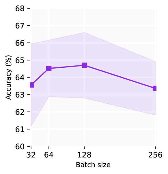
(a)

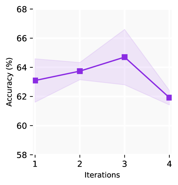
(b)

Figure 4: Impact of batch size (left) and the number of iterations for global alignment (right) on performance.

FedGaLA vs. FedAVG. In this experiment, we further evaluate the effectiveness of FedGaLA. To achieve this, after completing the aggregation process of FedGaLA, the global model is further updated using a combination of the weighted aggregated model and the FedAvg of the client models. This is formulated as:

$$\theta^{t+1}\leftarrow\gamma(\theta^{t}+\hat{\textbf{g}}^{t+1})+(1-\gamma)\text{FedAvg}(\theta_{i}^{t+1}),$$ (41)

where $\gamma$ is a parameter that balances the influence of the current aggregated update $\textbf{g}^{t+1}$ and the global model parameters obtained through FedAvg. FedAvg can be defined as $\theta^{t+1}=\theta^{t}+\frac{1}{N}\sum_{i=1}^{N}\tilde{w}_{i}\hat{\textbf{g}}_{i}^{t}$, where $\tilde{w}_{i}$ are the client weights, adjusted uniformly.

Table 6 shows the impact of $\gamma$ (introduced in Eq. (41) on performance. We observe that FedGaLA, i.e., $\gamma=1$, achieves the best results for all domains, except for the ‘Photo’ domain, where $\gamma=0.75$ yields the highest accuracy. It should be noted that with $\gamma=0.00$ the global alignment step of FedGaLA is effectively not performed, yielding the same performance observed in the second row of Table 3.

Table 6: Impact of $\gamma$ on performance.

$\gamma$	P	A	C	S	Ave.
1.00	64.7(1.9)	44.2(1.2)	60.5(2.2)	70.5(1.3)	60.0
0.75	65.4(1.7)	41.4(1.6)	59.8(2.4)	69.4(0.7)	58.9
0.50	64.9(1.3)	42.4(1.2)	59.2(1.9)	69.8(0.4)	59.1
0.25	64.8(1.2)	42.8(1.1)	59.7(1.2)	69.9(0.4)	59.3
0.00	64.7(0.4)	42.6(1.2)	58.1(0.6)	69.9(1.1)	58.8

Appendix F Additional discussion

Cross-silo vs. cross-device federated learning. Two frameworks can generally be considered in federated learning: cross-silo and cross-device. In cross-silo, the number of clients $K$ is small, and each client is capable of retaining its local model and state across training rounds. In contrast, cross-device federated learning works under the assumption of having millions of stateless clients, where only a limited number of clients participate in training during each communication round. However, due to limitations in experimental settings, the majority of studies typically conduct experiments involving at most hundreds of clients [57, 27]. In this study, given the limited number of domains FedGaLA works within the cross-silo framework. Moreover, each client is equipped with the necessary resources to participate in the collaborative learning process. Additionally, we ensure that every client updates its local model with a sufficient number of epochs.

Broader impact. This paper aims to advance the field of federated learning under realistic conditions of domain shift among clients and the absence of labeled data. While there are various potential societal implications of our work, we believe that the most notable is the advancement of decentralized privacy-preserving representation learning. Our approach enhances model generalization to new domains by aligning gradients across clients and the server. This leads to more accurate and robust models in areas such as the healthcare industry, where privacy is critical.

References

- [1] Brendan McMahan, Eider Moore, Daniel Ramage, Seth Hampson, and Blaise Aguera y Arcas. Communication-efficient learning of deep networks from decentralized data. In Artificial Intelligence and Statistics, pages 1273–1282, 2017.
- [2] Chen Zhang, Yu Xie, Hang Bai, Bin Yu, Weihong Li, and Yuan Gao. A survey on federated learning. Knowledge-Based Systems, 216:106775, 2021.
- [3] Avishek Ghosh, Jichan Chung, Dong Yin, and Kannan Ramchandran. An efficient framework for clustered federated learning. In Advances in Neural Information Processing Systems, volume 33, pages 19586–19597, 2020.
- [4] Zachary Charles, Zachary Garrett, Zhouyuan Huo, Sergei Shmulyian, and Virginia Smith. On large-cohort training for federated learning. Advances in Neural Information Processing Systems, 34:20461–20475, 2021.
- [5] Qinbin Li, Bingsheng He, and Dawn Song. Model-contrastive federated learning. In Proceedings of the IEEE/CVF Conference on Computer Vision and Pattern Recognition, pages 10713–10722, 2021.
- [6] Quande Liu, Cheng Chen, Jing Qin, Qi Dou, and Pheng-Ann Heng. FedDG: Federated domain generalization on medical image segmentation via episodic learning in continuous frequency space. In Proceedings of the IEEE/CVF Conference on Computer Vision and Pattern Recognition, pages 1013–1023, 2021.
- [7] Weiming Zhuang, Xin Gan, Yonggang Wen, Shuai Zhang, and Shuai Yi. Collaborative unsupervised visual representation learning from decentralized data. In Proceedings of the IEEE/CVF International Conference on Computer Vision, pages 4912–4921, 2021.
- [8] Liling Zhang, Xinyu Lei, Yichun Shi, Hongyu Huang, and Chao Chen. Federated learning with domain generalization. arXiv:2111.10487, 2021.
- [9] A Tuan Nguyen, Philip Torr, and Ser Nam Lim. FedSR: A simple and effective domain generalization method for federated learning. Advances in Neural Information Processing Systems, 35:38831–38843, 2022.
- [10] Ruqi Bai, Saurabh Bagchi, and David I. Inouye. Benchmarking algorithms for federated domain generalization. In The International Conference on Learning Representations, 2024.
- [11] Sungwon Han, Sungwon Park, Fangzhao Wu, Sundong Kim, Chuhan Wu, Xing Xie, and Meeyoung Cha. FedX: Unsupervised federated learning with cross knowledge distillation. In European Conference on Computer Vision, pages 691–707, 2022.
- [12] Samuel Yu, Peter Wu, Paul Pu Liang, Ruslan Salakhutdinov, and Louis-Philippe Morency. PACS: A dataset for physical audiovisual commonsense reasoning. In European Conference on Computer Vision, pages 292–309, 2022.
- [13] Hemanth Venkateswara, Jose Eusebio, Shayok Chakraborty, and Sethuraman Panchanathan. Deep hashing network for unsupervised domain adaptation. In Proceedings of the IEEE Conference on Computer Vision and Pattern Recognition, pages 5018–5027, 2017.
- [14] Xingchao Peng, Qinxun Bai, Xide Xia, Zijun Huang, Kate Saenko, and Bo Wang. Moment matching for multi-source domain adaptation. In Proceedings of the IEEE/CVF International Conference on Computer Vision, pages 1406–1415, 2019.
- [15] Sara Beery, Grant Van Horn, and Pietro Perona. Recognition in terra incognita. In Proceedings of the European Conference on Computer Vision, pages 456–473, 2018.
- [16] Tian Li, Anit Kumar Sahu, Manzil Zaheer, Maziar Sanjabi, Ameet Talwalkar, and Virginia Smith. Federated optimization in heterogeneous networks. Proceedings of Machine Learning and Systems, 2:429–450, 2020.
- [17] John Nguyen, Kshitiz Malik, Hongyuan Zhan, Ashkan Yousefpour, Mike Rabbat, Mani Malek, and Dzmitry Huba. Federated learning with buffered asynchronous aggregation. In International Conference on Artificial Intelligence and Statistics, pages 3581–3607, 2022.
- [18] Jianqing Zhang, Yang Hua, Hao Wang, Tao Song, Zhengui Xue, Ruhui Ma, and Haibing Guan. FedALA: Adaptive local aggregation for personalized federated learning. In Proceedings of the Association for the Advancement of Artificial Intelligence, volume 37, pages 11237–11244, 2023.
- [19] Ying Li, Xingwei Wang, Rongfei Zeng, Praveen Kumar Donta, Ilir Murturi, Min Huang, and Schahram Dustdar. Federated domain generalization: A survey. arXiv:2306.01334, 2023.
- [20] Guile Wu and Shaogang Gong. Collaborative optimization and aggregation for decentralized domain generalization and adaptation. In Proceedings of the IEEE/CVF International Conference on Computer Vision, pages 6484–6493, 2021.
- [21] Yuwei Sun, Ng Chong, and Hideya Ochiai. Feature distribution matching for federated domain generalization. In Asian Conference on Machine Learning, pages 942–957, 2023.
- [22] Junming Chen, Meirui Jiang, Qi Dou, and Qifeng Chen. Federated domain generalization for image recognition via cross-client style transfer. In Proceedings of the IEEE/CVF Winter Conference on Applications of Computer Vision, pages 361–370, 2023.
- [23] Jungwuk Park, Dong-Jun Han, Jinho Kim, Shiqiang Wang, Christopher G Brinton, and Jaekyun Moon. StableFDG: Style and attention based learning for federated domain generalization. Advances in Neural Information Processing Systems, 2023.
- [24] Ruipeng Zhang, Qinwei Xu, Jiangchao Yao, Ya Zhang, Qi Tian, and Yanfeng Wang. Federated domain generalization with generalization adjustment. In Proceedings of the IEEE/CVF Conference on Computer Vision and Pattern Recognition, pages 3954–3963, 2023.
- [25] Yilun Jin, Xiguang Wei, Yang Liu, and Qiang Yang. Towards utilizing unlabeled data in federated learning: A survey and prospective. arXiv:2002.11545, 2020.
- [26] Bram van Berlo, Aaqib Saeed, and Tanir Ozcelebi. Towards federated unsupervised representation learning. In Proceedings of the ACM International Workshop on Edge Systems, Analytics and Networking, pages 31–36, 2020.
- [27] Weiming Zhuang, Yonggang Wen, and Shuai Zhang. Divergence-aware federated self-supervised learning. In International Conference on Learning Representations, 2022.
- [28] Fengda Zhang, Kun Kuang, Long Chen, Zhaoyang You, Tao Shen, Jun Xiao, Yin Zhang, Chao Wu, Fei Wu, Yueting Zhuang, et al. Federated unsupervised representation learning. Frontiers of Information Technology & Electronic Engineering, 24(8):1181–1193, 2023.
- [29] Lucas Mansilla, Rodrigo Echeveste, Diego H Milone, and Enzo Ferrante. Domain generalization via gradient surgery. In Proceedings of the IEEE/CVF International Conference on Computer Vision, pages 6630–6638, 2021.
- [30] Aharon Bar-Hillel, Tomer Hertz, Noam Shental, and Daphna Weinshall. Learning distance functions using equivalence relations. In Proceedings of the International Conference on Machine Learning, pages 11–18, 2003.
- [31] Erik Štrumbelj and Igor Kononenko. Explaining prediction models and individual predictions with feature contributions. Knowledge and information systems, 41:647–665, 2014.
- [32] Erik Štrumbelj and Igor Kononenko. A general method for visualizing and explaining black-box regression models. In International Conference on Adaptive and Natural Computing Algorithms, pages 21–30. Springer, 2011.
- [33] Jiahui Yu and Konstantinos Spiliopoulos. Normalization effects on deep neural networks. arXiv preprint arXiv:2209.01018, 2022.
- [34] Haobo Qi, Jing Zhou, and Hansheng Wang. A note on factor normalization for deep neural network models. Scientific Reports, 12(1):5909, 2022.
- [35] Lei Huang, Jie Qin, Yi Zhou, Fan Zhu, Li Liu, and Ling Shao. Normalization techniques in training dnns: Methodology, analysis and application. IEEE Transactions on Pattern Analysis and Machine Intelligence, 2023.
- [36] Ting Chen, Simon Kornblith, Mohammad Norouzi, and Geoffrey Hinton. A simple framework for contrastive learning of visual representations. In International Conference on Machine Learning, pages 1597–1607, 2020.
- [37] Zihao Wang, Chunxu Wu, Yifei Yang, and Zhen Li. Learning transformation-predictive representations for detection and description of local features. In Proceedings of the IEEE/CVF Conference on Computer Vision and Pattern Recognition, pages 11464–11473, 2023.
- [38] Jian Gao, Yang Hua, Guosheng Hu, Chi Wang, and Neil M Robertson. Reducing distributional uncertainty by mutual information maximisation and transferable feature learning. In European Conference on Computer Vision, pages 587–605, 2020.
- [39] Willi Menapace, Stéphane Lathuilière, and Elisa Ricci. Learning to cluster under domain shift. In Proceedings of the European Conference on Computer Vision, pages 736–752, 2020.
- [40] Zijian Wang, Yadan Luo, Ruihong Qiu, Zi Huang, and Mahsa Baktashmotlagh. Learning to diversify for single domain generalization. In Proceedings of the IEEE/CVF International Conference on Computer Vision, pages 834–843, 2021.
- [41] Ziv Goldfeld and Kristjan Greenewald. Sliced mutual information: A scalable measure of statistical dependence. Advances in Neural Information Processing Systems, 34:17567–17578, 2021.
- [42] Yuge Shi, Jeffrey Seely, Philip Torr, Siddharth N, Awni Hannun, Nicolas Usunier, and Gabriel Synnaeve. Gradient matching for domain generalization. In International Conference on Learning Representations, 2022.
- [43] Alexandre Rame, Corentin Dancette, and Matthieu Cord. Fishr: Invariant gradient variances for out-of-distribution generalization. In International Conference on Learning Representations, 2022.
- [44] Da Li, Yongxin Yang, Yi-Zhe Song, and Timothy M Hospedales. Deeper, broader and artier domain generalization. In Proceedings of the IEEE International Conference on Computer Vision, pages 5542–5550, 2017.
- [45] Xingxuan Zhang, Linjun Zhou, Renzhe Xu, Peng Cui, Zheyan Shen, and Haoxin Liu. Towards unsupervised domain generalization. In Proceedings of the IEEE/CVF Conference on Computer Vision and Pattern Recognition, pages 4910–4920, 2022.
- [46] Ishaan Gulrajani and David Lopez-Paz. In search of lost domain generalization. In International Conference on Learning Representations, 2021.
- [47] Zeyu Feng, Chang Xu, and Dacheng Tao. Self-supervised representation learning from multi-domain data. In Proceedings of the IEEE/CVF International Conference on Computer Vision, pages 3245–3255, 2019.
- [48] Richard Zhang, Phillip Isola, and Alexei A Efros. Split-brain autoencoders: Unsupervised learning by cross-channel prediction. In Proceedings of the IEEE Conference on Computer Vision and Pattern Recognition, pages 1058–1067, 2017.
- [49] Alexander Kolesnikov, Xiaohua Zhai, and Lucas Beyer. Revisiting self-supervised visual representation learning. In Proceedings of the IEEE/CVF Conference on Computer Vision and Pattern Recognition, pages 1920–1929, 2019.
- [50] Kaiming He, Haoqi Fan, Yuxin Wu, Saining Xie, and Ross Girshick. Momentum contrast for unsupervised visual representation learning. In Proceedings of the IEEE/CVF Conference on Computer Vision and Pattern Recognition, pages 9729–9738, 2020.
- [51] Jean-Bastien Grill, Florian Strub, Florent Altché, Corentin Tallec, Pierre Richemond, Elena Buchatskaya, Carl Doersch, Bernardo Avila Pires, Zhaohan Guo, Mohammad Gheshlaghi Azar, et al. Bootstrap your own latent-a new approach to self-supervised learning. Advances in Neural Information Processing Systems, 33:21271–21284, 2020.
- [52] Qianjiang Hu, Xiao Wang, Wei Hu, and Guo-Jun Qi. Adco: Adversarial contrast for efficient learning of unsupervised representations from self-trained negative adversaries. In Proceedings of the IEEE/CVF Conference on Computer Vision and Pattern Recognition, pages 1074–1083, 2021.
- [53] Kaiming He, Xiangyu Zhang, Shaoqing Ren, and Jian Sun. Deep residual learning for image recognition. In Proceedings of the IEEE Conference on Computer Vision and Pattern Recognition, pages 770–778, 2016.
- [54] Soroosh Tayebi Arasteh, Christiane Kuhl, Marwin-Jonathan Saehn, Peter Isfort, Daniel Truhn, and Sven Nebelung. Mind the gap: Federated learning broadens domain generalization in diagnostic ai models. arXiv:2310.00757, 2023.
- [55] Xinlei Chen and Kaiming He. Exploring simple siamese representation learning. In Proceedings of the IEEE/CVF Conference on Computer Vision and Pattern Recognition, pages 15750–15758, 2021.
- [56] Diederik P Kingma and Jimmy Ba. Adam: A method for stochastic optimization. arXiv:1412.6980, 2014.
- [57] Hongyi Wang, Mikhail Yurochkin, Yuekai Sun, Dimitris Papailiopoulos, and Yasaman Khazaeni. Federated learning with matched averaging. In International Conference on Learning Representations, 2020.