Layer-Aware Analysis of Catastrophic Overfitting:
Revealing the Pseudo-Robust Shortcut Dependency

Abstract

Catastrophic overfitting (CO) presents a significant challenge in single-step adversarial training (AT), manifesting as highly distorted deep neural networks (DNNs) that are vulnerable to multi-step adversarial attacks. However, the underlying factors that lead to the distortion of decision boundaries remain unclear. In this work, we delve into the specific changes within different DNN layers and discover that during CO, the former layers are more susceptible, experiencing earlier and greater distortion, while the latter layers show relative insensitivity. Our analysis further reveals that this increased sensitivity in former layers stems from the formation of pseudo-robust shortcuts, which alone can impeccably defend against single-step adversarial attacks but bypass genuine-robust learning, resulting in distorted decision boundaries. Eliminating these shortcuts can partially restore robustness in DNNs from the CO state, thereby verifying that dependence on them triggers the occurrence of CO. This understanding motivates us to implement adaptive weight perturbations across different layers to hinder the generation of pseudo-robust shortcuts, consequently mitigating CO. Extensive experiments demonstrate that our proposed method, Layer-Aware Adversarial Weight Perturbation (LAP), can effectively prevent CO and further enhance robustness. Our implementation can be found at https://github.com/tmllab/2024_ICML_LAP.

1 Introduction

Standard adversarial training (AT) (Madry et al., 2018; Zhang et al., 2019) is widely acknowledged as the most effective method for improving the robustness of deep neural networks (DNNs) (Athalye et al., 2018; Croce et al., 2022). Nevertheless, this training approach significantly increases the computational overhead due to the multi-step backward propagation, which limits its scalability for large networks and datasets. To alleviate this issue, several works (Shafahi et al., 2019; Wong et al., 2019; Kim et al., 2021) have introduced single-step AT as a time-efficient alternative, offering a balance between practicality and robustness.

Figure 1: The test accuracy of R-FGSM and R-LAP under 16/255 noise magnitude, where the solid and dashed lines denote natural and robust (PGD) accuracy, respectively.

Unfortunately, single-step AT faces a critical challenge known as catastrophic overfitting (CO) (Wong et al., 2019). This intriguing phenomenon is characterized by a sharp decline in the DNN’s robustness, plummeting from peak to nearly zero in just a few iterations, as illustrated in Figure 1. Prior studies (Andriushchenko & Flammarion, 2020; Kim et al., 2021) have pointed out that classifiers suffering from CO typically exhibit severely distorted decision boundaries. This distortion leads to a strange performance paradox in models affected by CO, as they can perfectly defend against single-step adversarial attacks but are highly vulnerable to multi-step adversarial attacks. However, the precise process of decision boundary distortion and the underlying factors that contribute to this performance paradox remain unclear.

To gain a detailed investigation of CO, we analyse the specific changes within individual DNN layers and their respective influences on the distortion of decision boundaries. More specifically, we identify the distinct transformations occurring in different layers during the CO process. The initial alterations in the DNN primarily occur in the former layers, leading to observable distorted decision boundaries and a subsequent reduction in robustness. As training progresses, each layer within DNNs experiences varying degrees of distortion. Notably, the former layers are more susceptible, showing markedly pronounced distortion, whereas the latter layers display relative resilience. As a result, forward propagation through these distorted former layers leads the model to exhibit sharp decision boundaries and manifest as CO.

Building on this, we delve into the underlying factors driving the transformation process that results in the distortion of decision boundaries and the performance paradox. Our research reveals that the heightened sensitivity in DNN’s former layers can be attributed to the generation of pseudo-robust shortcuts. These shortcuts, associated with certain large weights, empower the model to attain exceptional performance defence against single-step adversarial attacks. Nevertheless, relying solely on these shortcuts for decision-making induces the model to bypass genuine-robust learning, consequently distorting decision boundaries. By removing large weights from the former layers, we can effectively disrupt the improper reliance on these pseudo-robust shortcuts, thereby gradually reinstating the robustness of DNNs in the CO state. The above analyses validate that the model’s dependence on pseudo-robust shortcuts for decision-making is the key factor triggering the occurrence of CO.

Motivated by these insights, our proposed method, Layer-Aware Adversarial Weight Perturbation (LAP), is designed to prevent CO by hindering the generation of pseudo-robust shortcuts. To realize this objective, LAP is strategically crafted to interrupt the model’s stable reliance on these shortcuts by explicitly implementing adaptive weight perturbations across different layers. It is worth noting that our method simultaneously generates adversarial perturbations for both inputs and weights, thus avoiding any additional computational burden. We evaluate the effectiveness of our method across various adversarial attacks, datasets, and network architectures, showing that our proposed method can not only effectively eliminate CO but also further boost adversarial robustness, even under extreme noise magnitudes. Our main contributions are summarized as follows:

• We find that during CO, different layers undergo distinct changes, with the former layers exhibiting greater sensitivity, marked by earlier and more significant distortion.

• We reveal that the generation and dependence on pseudo-robust shortcuts trigger CO, which allows the model to precisely defend against single-step adversarial attacks but bypass genuine-robustness learning.

• We propose the LAP method, which aims to obstruct the formation of pseudo-robust shortcuts, thereby effectively preventing the occurrence of CO.

2 Related Work

In this section, we briefly review the relevant literature.

2.1 Adversarial Training

AT has been demonstrated to be the most effective defence method (Athalye et al., 2018; Zhou et al., 2022; Dong et al., 2023) that is generally formulated as a min-max optimization problem (Madry et al., 2018; Croce et al., 2022; Wang et al., 2024), which is shown in the following formula:

$$\min_{\mathbf{w}}\mathbb{E}_{\left\{\mathbf{x}_{i},y_{i}\right\}_{i=1}^{n}}\left[\max_{\delta_{i}\in\epsilon_{p}}\ell(f_{\mathbf{w}}(x_{i}+\delta_{i}),y_{i})\right],$$ (1)

where $\{\mathbf{x}_{i},y_{i}\}_{i=1}^{n}$ is the training dataset, $f$ is the classifier parameterized by $\mathbf{w}$, $\ell$ is the cross-entropy loss, $\delta$ is the perturbation confined within the $\epsilon$ radius $L_{p}$-norm ball.

Vanilla Fast Gradient Sign Method (V-FGSM) (Goodfellow et al., 2014) is a single-step maximization approach that utilizes one iteration to generate perturbations, defined as:

$$\delta_{V-FGSM}=\epsilon\cdot\operatorname{sign}\left(\nabla_{x}\ell(f_{\mathbf{w}}(x_{i}),y_{i})\right).$$ (2)

Random FGSM (R-FGSM) (Wong et al., 2019) and Noise FGSM (N-FGSM) (de Jorge Aranda et al., 2022) adopt stronger noise initialization $(-\epsilon,\epsilon)$ and $(-2\epsilon,2\epsilon)$, respectively, to further enhance the quality of maximization.

To improve robust generalization, Adversarial Weight Pertuabtion (AWP) (Wu et al., 2020) introduces an extra weight perturbation process, which is formulated as follows:

$$\min_{\mathbf{w}}\max_{\boldsymbol{\nu}\in\mathcal{V}}\frac{1}{n}\sum_{i=1}^{n}\max_{\delta_{i}\in\epsilon_{p}}\ell\left(f_{\mathbf{w}+\boldsymbol{\nu}}(x_{i}+\delta_{i}),y_{i})\right),$$ (3)

where $\mathcal{V}$ is a feasible region for the weight perturbation $\boldsymbol{\nu}$.

2.2 Weight Perturbation

The relationship between the geometry of the loss landscape and the model’s generalization ability has been widely investigated (Keskar et al., 2016; Dziugaite & Roy, 2017; Huang et al., 2023b; Li & Spratling, 2023). Recent works have demonstrated that random weight perturbations can effectively smooth the loss surface, thereby enhancing the generalization capacity (Wen et al., 2018; He et al., 2019). Building on this, several studies have utilized gradient information to generate adversarial weight perturbations, aiming to flatten the landscape in worst-case scenarios (Wu et al., 2020; Foret et al., 2020; Yu et al., 2022a, b). However, the impact of weight perturbation across different layers, as well as its role in CO, remains rarely explored.

Figure 2: Visualization of the loss landscape for individual layers (1st to 5th columns) and for the whole model (6th column). The upper, middle, and lower rows correspond to the stages before, during, and after CO, respectively.

2.3 Catastrophic Overfitting

Since the identification of CO (Wong et al., 2019), a line of studies has been dedicated to understanding and addressing this intriguing phenomenon. de Jorge Aranda et al. (2022); Niu et al. (2022) found that employing a stronger noise initialization can effectively delay the onset of CO. Additionally, Andriushchenko & Flammarion (2020) observed that the models impacted by CO tend to become highly distorted and proposed a gradient align method to smooth local non-linear surfaces. Recent works have also introduced a variety of strategies designed to counter CO, including subspace extraction (Li et al., 2022), gradient filtering (Vivek & Babu, 2020; Golgooni et al., 2023; Lin et al., 2023a), adaptive perturbation (Kim et al., 2021; Huang et al., 2023a), and local linearity (Park & Lee, 2021; Sriramanan et al., 2021; Lin et al., 2023b; Rocamora et al., 2023). Regrettably, the aforementioned methods either suffer from CO when faced with stronger adversaries or significantly increase the computational overhead. This study explores the changes within individual DNN layers and introduces a pseudo-robust shortcuts dependency perspective, thereby proposing the LAP as an effective and efficient CO solution.

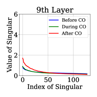
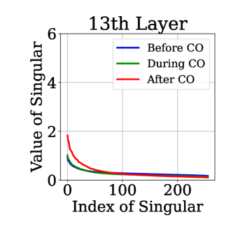
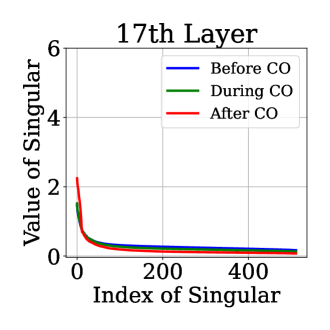
Figure 3: Singular value of weights (convolution kernel) at different DNN layers. The blue, green, and red lines represent the model state before, during, and after CO, respectively.

3 Methodology

In this section, we observe that during catastrophic overfitting (CO), different layers in deep neural networks (DNNs) undergo distinct changes, with the former layers being more prone to distortion (Section 3.1). Subsequently, we reveal that the model’s reliance on pseudo-robust shortcuts for decision-making triggers CO (Section 3.2). Consequently, we propose Layer-Aware Adversarial Weight Perturbation (LAP), which applies adaptive perturbations to eliminate the generation of shortcuts (Section 3.3). Finally, we provide a theoretical analysis deriving an upper bound to ensure the effectiveness of our proposed method (Section 3.4).

3.1 Layers Transformation During CO

Prior research (Andriushchenko & Flammarion, 2020; Kim et al., 2021) has shown that the decision boundaries of DNNs undergo significant distortion during the CO process, resulting in a performance paradox in response to single-step and multi-step adversarial attacks. Nevertheless, the prevailing studies on CO generally consider DNNs as a whole and focus on analysing the final output. However, considering an L-layer DNN with parameters $\{\mathbf{w}_{l}\}_{l=1}^{L}$, its output is an aggregation of forward propagation through these layers, denoted by $f_{\mathbf{w}}(x)=\mathbf{w}_{L}(\mathbf{w}_{L-1}\ldots(\mathbf{w}_{1}x))$ for $l=1,\ldots,L$. Therefore, the specific impact of each layer on the distorted decision boundaries and the underlying factors that induce this performance paradox are still unclear.

In this work, we conduct a layer-by-layer investigation of the single-step AT throughout the training process, as illustrated in Figure 2. Specifically, we utilize a PreActResNet-18 network trained on the CIFAR-10 dataset using the R-FGSM (Wong et al., 2019) method under 16/255 noise magnitude. For visualizing the loss landscape of the whole model, we apply random perturbations to the input, denoted as $x+\delta$, and then compute the variation in loss, represented as $\Delta$ Loss. To analyse individual layers, we introduce random perturbations to the weights of the corresponding layer, expressed as $\mathbf{w}_{l}+\delta$ for $l=1,5,9,13,17$, and calculate the subsequent change in the loss.

As illustrated in Figure 2 (upper row), at the moment of peak robustness, both the whole model and its individual layers exhibit a flattened loss landscape. At this point, it becomes evident that the former layers display a higher degree of stability compared to the latter layers, as indicated by the smaller variations in loss due to the random perturbations.

With the onset of CO, the model manifests a decrease in robustness, accompanied by an observable distortion in the loss landscape, as illustrated in Figure 2 (middle row). The detailed analysis within each layer demonstrates that the former layers are the first to manifest increased sensitivity, characterized by a sharper loss landscape; in contrast, the latter layers undergo only minor transformations.

Following the occurrence of CO, the classifier’s decision boundaries become completely distorted, rendering it extremely vulnerable to multi-step adversarial attacks, as depicted in Figure 2 (lower row). It can be observed that different layers exhibit distinct changes; the former layers experience the most severe distortion, marked by a significantly sharp surface, whereas the latter layers exhibit relative insensitivity. In summary, during the CO process, the former layers within DNNs undergo the most profound changes, transitioning from relatively stable to entirely sensitive.

3.2 Pseudo-Robust Shortcut Dependency

Subsequently, we delve into the underlying factors that induce the sensitivity transformation observed in DNNs during the CO process. To accomplish this objective, we examine the influence of weights on the model’s decision-making process. In practice, we compute the singular values for each convolutional kernel to handle the extensive number of weights, as depicted in Figure 3. Before the CO occurrence, a fairly uniform distribution of singular values is observed across all layers. However, after CO, there is a noticeable increase in the variance of singular values, leading to sharper model output, as discussed in Section 3.1. This significant rise in large singular values suggests the growing importance of certain weights in the model’s decision-making. Remarkably, the former layers exhibit the most pronounced increase in large singular values, nearly tripling from before, indicating that the model’s decision-making becomes heavily dependent on certain weights in these layers.

In order to gain deeper insight into this dependency, we randomly removed some weights from the former (1st to 5th) layers in a model already affected by CO, as illustrated in Figure 4(a) (left column). With the increased removal rate, the model’s accuracy under the FGSM attack decreased from 26% to 6%, whereas its accuracy against the PGD attack showed a slight increase. This anomalous trend indicates a performance paradox in models impacted by CO under FGSM and PGD attacks, contrasting with genuine-robust models where higher FGSM accuracy generally implies greater PGD accuracy. Therefore, we propose that the heightened sensitivity in the former layers originates from the generation of pseudo-robust shortcuts, solely relying on them can effectively defend against single-step adversarial attacks but bypass genuine-robust learning.

To further substantiate our perspective, we investigate the particular weights associated with these pseudo-robust shortcuts. As shown in Figure 4(a) (middle column), the removal of small weights in the former layers has a negligible impact on the model’s performance against both FGSM and PGD attacks, suggesting a weak relevance between these weights and shortcuts. Conversely, removing only 10% of the large weights can effectively interrupt the pseudo-robust shortcuts, resulting in a notable 22% reduction in FGSM attack accuracy and reinstatement of robustness against PGD attack to 2.65%, as depicted in Figure 4(a) (right column). With the gradual removal of larger weights, the model not only shows an improvement in robustness but also successfully overcomes the performance paradox against FGSM and PGD attacks. For a fair comparison, we also remove the large weights from the latter (14th to 17th) layers, as depicted in Figure 4(b). Clearly, the same intervention in the latter layers is less effective, highlighting the pseudo-robust shortcuts that play a critical role in the CO phenomenon, primarily present in the former layer.

Conclusively, we introduce the perspective of pseudo-robust shortcuts dependency to explain the occurrence of CO. Specifically, the heightened sensitivity of DNN can be attributed to its decision-making solely dependent on pseudo-robust shortcuts, which are typically associated with certain large weights in former layers. These shortcuts, although exceptionally accurate in defending against single-step adversarial attacks, induce the model to bypass genuine-robust learning, thereby resulting in distorted decision boundaries and triggering the performance paradox in CO.

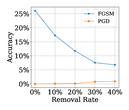
(a) Remove random weights, small weights, and large weights from the former (1st to 5th) layers, as shown in the left, middle, and right columns, respectively.

(b) Remove large weights from the latter (14th to 17th) layers.

Figure 4: Evaluating the test accuracy of a CO-affected model against single-step (FGSM) and multi-step (PGD) adversarial attack.

3.3 Proposed Methods

Building upon our perspective, our objective is to eliminate the formation of pseudo-robust shortcuts, thereby effectively preventing the occurrence of CO. Inspired by AWP (Wu et al., 2020) and SAM (Foret et al., 2020), we introduce the Layer-Aware Adversarial Weight Perturbation (LAP) method that explicitly implements adaptive weight perturbations across different layers to hinder the generation of pseudo-robust shortcuts, which can be expressed as follows:

$$\min_{\mathbf{w}}\frac{1}{n}\sum_{i=1}^{n}\max_{\delta_{i}}\max_{\boldsymbol{\nu}_{l}}\ell\left(f_{\mathbf{w}+\boldsymbol{\nu}_{l}}(x_{i}+\delta_{i}),y_{i})\right).$$ (4)

To closely align with our goal, we introduce three novel improvements. Firstly, our method accumulates weight perturbations to effectively break persistent shortcuts by maintaining a larger magnitude of alteration. Secondly, we prioritize generating weight perturbations over input perturbations, aiming to obstruct the model from establishing stable shortcuts between inputs and weights. Thirdly, recognizing the distinct transformations in each layer, our approach adopts a gradually decreasing weight perturbation strategy from the former to the latter layer to avoid unnecessary redundant perturbations, as summarized below:

$$\lambda_{l}=\beta\cdot\left(1-\left(\frac{\ln(l)}{\ln(L+1)}\right)^{\gamma}\right),\,\,\,\text{for }l=1,\ldots,L$$ (5)

where $\lambda_{l}$ is the layer-aware perturbation, $\beta$ is the step size, and $\gamma$ controls the different layers strength.

However, the above design still requires extra backward propagation, which diminishes the efficiency advantage of single-step AT. To address this issue, we propose an efficient LAP implementation that concurrently generates adversarial perturbations for both inputs and weights, as detailed below:

$$\min_{\mathbf{w}}\frac{1}{n}\sum_{i=1}^{n}\max_{\delta_{i},\boldsymbol{\nu}_{l}}\ell\left(f_{\mathbf{w}+\boldsymbol{\nu}_{l}}(x_{i}+\delta_{i}),y_{i})\right).$$ (6)

We further elucidate the intuitive basis for the efficient implementation of LAP. For a given input, its corresponding adversarial perturbation is generated by maximizing the loss value, which is calculated from both the network weights and the loss function. Assuming the loss function is Lipschitz continuous with a constant $\mathbb{L}$, the change in loss due to weight perturbation can be bounded as follows:

$$\left|\ell\left(f_{\mathbf{w}+\nu_{l}}(x),y\right)-\ell\left(f_{\mathrm{w}}(x),y\right)\right|\leq\mathbb{L}\left\|f_{\mathbf{w}+\nu_{l}}(x)-f_{\mathbf{w}}(x)\right\|.$$ (7)

Hence, the variation in loss value is directly related to the changes in the model’s output, which results from the aggregation of multiple layers, as outlined below:

$$f_{\mathbf{w}+\boldsymbol{\nu}_{l}}(x)-f_{\mathbf{w}}(x)=\prod_{l=1}^{L}(\mathbf{w}_{l}+\boldsymbol{\nu}_{l})\cdot x-\prod_{l=1}^{L}(\mathbf{w}_{l})\cdot x.$$ (8)

The above analysis reveals a positive correlation between changes in output and the magnitudes of weight perturbations. In practice, we employ a small weight perturbation size to restrict this magnitude. Meanwhile, our optimization objective is to attain a flattened weight loss landscape, ensuring that the introduction of small weight perturbations leads to relatively minor alterations in the loss value. Therefore, this discussion empirically demonstrates that the input perturbation, generated based on the original weights, has a high probability of retaining its effectiveness after the injection of weight perturbations, consequently enabling us to simultaneously generate both input and weight perturbations. The LAP algorithm is summarized in Algorithm 1.

Algorithm 1 Layer-Aware Adversarial Weight Perturbation

0:  L-layer Network $f_{\mathbf{w}}$, training data $\{\mathbf{x}_{i},y_{i}\}_{i=1}^{n}$, training epoch $T$, batch size $N$, input perturbation size $\alpha$, layer-aware weight perturbation size $\lambda_{l}$.

0:  Adversarially robust model $f_{\mathbf{w}}$.

1:  for $t=1\ldots T$ to do

2:     for $i=1\ldots N$ to do

3:        # simultaneously generate $\delta_{i}$ and $\boldsymbol{\nu}_{l}$.

4:        $\delta_{i}=\alpha\cdot\operatorname{sign}\left(\nabla_{x}\ell(f_{\mathbf{w}}(x_{i}),y_{i})\right)$

5:        $\boldsymbol{\nu}_{l}=\lambda_{l}\cdot\frac{\nabla_{\mathbf{w}}\ell\left(f_{\mathbf{w}}(x_{i}),y_{i})\right)}{\left\|\nabla_{\mathbf{w}}\ell\left(f_{\mathbf{w}}(x_{i}),y_{i})\right)\right\|}\|\mathbf{w}\|$

6:        $LAP=\frac{1}{n}\sum_{i=1}^{n}\ell\left(f_{\mathbf{w}+\boldsymbol{\nu}_{l}}(x_{i}+\delta_{i}),y_{i})\right)$

7:        $\mathbf{w}=(\mathbf{w}+\boldsymbol{\nu}_{l})-\nabla_{\mathbf{w}+\boldsymbol{\nu}_{l}}\left(LAP\right)$

8:     end for

9:  end for

Table 1: Comparison of CIFAR-10 test accuracy (%) for various methods under different noise magnitudes. The results are averaged over three random seeds and reported with the standard deviation.

Method	8/255			12/255			16/255			32/255
	Natural	Auto Attack		Natural	Auto Attack		Natural	Auto Attack		Natural	Auto Attack
AT Free	76.52$\pm$1.34	40.13$\pm$0.39		68.28$\pm$0.13	27.65$\pm$0.38		55.91$\pm$10.94	0.00$\pm$0.00		59.25$\pm$10.98	0.00$\pm$0.00
Grad Align	82.35$\pm$0.92	44.76$\pm$0.02		74.80$\pm$0.64	29.88$\pm$0.23		61.10$\pm$0.49	19.07$\pm$0.28		24.15$\pm$4.03	6.71$\pm$2.31
ZeroGrad	81.71$\pm$0.21	43.28$\pm$0.18		77.75$\pm$0.20	22.56$\pm$0.05		82.54$\pm$0.19	0.00$\pm$0.00		68.95$\pm$2.51	0.00$\pm$0.00
MultiGrad	81.83$\pm$0.31	44.19$\pm$0.10		83.72$\pm$1.47	0.00$\pm$0.00		81.59$\pm$3.19	0.00$\pm$0.00		73.50$\pm$4.90	0.00$\pm$0.00
V-FGSM	84.26$\pm$4.18	0.00$\pm$0.00		79.92$\pm$1.82	0.00$\pm$0.00		72.72$\pm$3.04	0.00$\pm$0.00		65.52$\pm$2.15	0.00$\pm$0.00
V-LAP	79.09$\pm$0.78	41.24$\pm$0.51		66.20$\pm$0.42	24.07$\pm$0.34		56.02$\pm$0.07	15.17$\pm$0.31		17.76$\pm$3.11	7.12$\pm$0.64
R-FGSM	84.12$\pm$0.29	42.88$\pm$0.09		79.49$\pm$4.57	0.00$\pm$0.00		73.67$\pm$6.86	0.00$\pm$0.00		33.31$\pm$8.31	0.00$\pm$0.00
R-LAP	83.81$\pm$0.24	43.14$\pm$0.45		74.10$\pm$0.31	26.04$\pm$1.04		64.83$\pm$0.29	15.69$\pm$0.28		27.49$\pm$0.48	8.04$\pm$0.63
N-FGSM	80.40$\pm$0.16	44.21$\pm$0.47		71.44$\pm$0.16	30.25$\pm$0.06		62.91$\pm$1.03	18.58$\pm$2.28		27.66$\pm$3.57	0.00$\pm$0.00
N-LAP	80.76$\pm$0.15	44.97$\pm$0.24		71.91$\pm$0.19	30.60$\pm$0.27		63.73$\pm$0.27	19.55$\pm$0.18		29.19$\pm$1.00	8.85$\pm$1.48
PGD-2	84.72$\pm$0.08	42.92$\pm$0.60		79.13$\pm$0.25	28.30$\pm$0.35		72.50$\pm$0.51	17.89$\pm$0.16		48.99$\pm$0.19	3.76$\pm$0.02
PGD-10	80.91$\pm$0.52	46.37$\pm$0.76		72.03$\pm$0.30	33.13$\pm$0.28		67.61$\pm$0.83	21.98$\pm$0.30		35.28$\pm$0.78	10.88$\pm$0.41

3.4 Theoretical Analysis

Furthermore, we provide a theoretical analysis to derive an upper bound on the expected error of our method. Building upon the previous PAC-Bayesian framework (Neyshabur et al., 2017; Wu et al., 2020) and assuming a prior distribution $\mathbb{P}\sim\mathcal{N}(0,\sigma^{2})$ for the weights, we can formulate the upper bound for the expected error of the classifier, with a probability of at least $1-\delta$ across the $n$ training samples:

$$\mathbb{E}_{\boldsymbol{\nu}}\left[\ell\left(f_{\mathbf{w}+\boldsymbol{\nu}}\right)\right] \leq{\mathbb{E}_{\boldsymbol{\nu}}\left[\hat{\ell}\left(f_{\mathbf{w}+\boldsymbol{\nu}}\right)\right]}$$ (9)

$$+4\sqrt{\frac{1}{n}\left(KL(\mathbf{w}+\boldsymbol{\nu}\|P)+\ln\frac{2n}{\delta}\right)}.$$

Considering the weight perturbation in the worst-case scenario $max_{\boldsymbol{\nu}}[\hat{\ell}\left(f_{\mathbf{w}+\boldsymbol{\nu}}\right)]$, and the standard deviation of the weight perturbation relation to the layer magnitude $\sigma_{l}=\lambda_{l}\cdot\|\mathbf{w}_{l}\|_{2}$, the PAC-Bayes bound of our proposed LAP method can be controlled as follows:

$$\mathbb{E}_{\left\{\mathbf{x}_{i},y_{i}\right\}_{i=1}^{n},\{\boldsymbol{\nu}_{l}\}_{l=1}^{L}} [\ell\left(f_{\mathbf{w}+\boldsymbol{\nu}_{l}}\right)]\leq\hat{\ell}\left(f_{\mathbf{w}}\right)$$ (10)

$$\!\!\!\!\!\!\!\!\!\!\!\!\!\!\!\!\!+\left\{max_{\{\boldsymbol{\nu}_{l}\}_{l=1}^{L}}[\hat{\ell}\left(f_{\mathbf{w}+\boldsymbol{\nu}_{l}}\right)]-\hat{\ell}\left(f_{\mathbf{w}}\right)\right\}$$

$$\!\!\!\!\!\!\!\!\!\!\!\!\!\!\!\!\!+4\sqrt{\frac{1}{n}\left(\sum_{l=1}^{L}\left(\frac{1}{2\lambda_{l}^{2}}\right)+\ln\frac{2n}{\delta}\right)}.$$

4 Experiment

In this section, we evaluate the effectiveness of LAP, including experiment settings (Section 4.1), performance evaluations (Section 4.2), ablation studies (Section 4.3), and training cost analysis (Section 4.4).

4.1 Experiment Setting

Table 2: Comparison of CIFAR-100 test accuracy (%) for various methods under different noise magnitudes. The results are averaged over three random seeds and reported with the standard deviation.

Method	8/255			12/255			16/255			32/255
	Natural	Auto Attack		Natural	Auto Attack		Natural	Auto Attack		Natural	Auto Attack
V-FGSM	54.87$\pm$2.53	0.00$\pm$0.00		45.40$\pm$1.89	0.00$\pm$0.00		41.38$\pm$6.03	0.00$\pm$0.00		27.22$\pm$4.54	0.00$\pm$0.00
V-LAP	53.07$\pm$0.59	19.49$\pm$0.57		42.24$\pm$0.29	11.27$\pm$0.33		34.30$\pm$0.19	7.63$\pm$0.52		9.37$\pm$1.76	1.33$\pm$0.21
R-FGSM	60.29$\pm$2.12	0.00$\pm$0.00		21.18$\pm$9.56	0.00$\pm$0.00		11.46$\pm$7.33	0.00$\pm$0.00		13.56$\pm$10.95	0.00$\pm$0.00
R-LAP	58.75$\pm$0.20	21.62$\pm$0.01		49.74$\pm$0.29	12.10$\pm$0.13		39.13$\pm$0.46	7.98$\pm$1.09		19.52$\pm$0.84	2.50$\pm$0.44
N-FGSM	55.19$\pm$0.35	22.46$\pm$0.12		46.16$\pm$0.18	14.51$\pm$0.11		37.71$\pm$0.06	10.22$\pm$0.18		18.29$\pm$5.64	0.00$\pm$0.00
N-LAP	55.12$\pm$0.20	23.15$\pm$0.28		46.76$\pm$0.18	15.16$\pm$0.04		38.02$\pm$0.11	10.40$\pm$0.14		16.85$\pm$0.83	3.45$\pm$0.28
PGD-2	60.09$\pm$0.20	22.52$\pm$0.14		53.46$\pm$0.27	13.69$\pm$0.02		47.50$\pm$0.28	9.56$\pm$0.07		31.89$\pm$0.69	1.76$\pm$0.22
PGD-10	55.20$\pm$0.31	23.71$\pm$0.11		47.74$\pm$0.15	15.52$\pm$0.06		42.21$\pm$0.16	10.87$\pm$0.07		21.82$\pm$0.21	4.03$\pm$0.08

Figure 5: Visualization of the loss landscape for individual layers (1st to 5th columns) and for the whole model (6th column).

Baselines.  We select a range of popular single-step AT methods for compare with LAP, which includes V-FGSM (Goodfellow et al., 2014), R-FGSM (Wong et al., 2019), N-FGSM (de Jorge Aranda et al., 2022), FreeAT (Shafahi et al., 2019), Grad Align (Andriushchenko & Flammarion, 2020), ZeroGrad and MultiGrad (Golgooni et al., 2023). Additionally, we present the results of the iterative-step AT method PGD-2 and PGD-10 (Madry et al., 2018) as a reference for ideal performance.

Datasets and Model Architectures.  We use three benchmark datasets, CIFAR-10, CIFAR-100 (Krizhevsky et al., 2009) and Tiny-ImageNet (Netzer et al., 2011), for evaluating the performances of our proposed method. The widely-used data augmentation random cropping and horizontal flipping are applied to these datasets. The settings and results on Tiny-ImageNet can be found in Appendix B. For a comprehensive evaluation, we report the training from scratch results on PreActResNet-18 (He et al., 2016), WideResNet-34 (Zagoruyko & Komodakis, 2016), and Vit-small (Dosovitskiy et al., 2020) architectures. The results of WideResNet-34 and Vit-small are provided in Appendix A.

Learning Rate Schedule.  We use the cyclical learning rate schedule (Smith, 2017) spanning 30 epochs, which reaches its maximum learning rate of 0.2 at the 15th epoch. The results of the piecewise learning rate schedule with 200 training epochs are available in Appendix C.

Adversarial Evaluation.  In order to thoroughly assess the models’ robustness, we utilize the widely-used PGD attack configuration with 50 steps and 10 restarts (Wong et al., 2019), as well as the Auto Attack (Croce & Hein, 2020).

Setup for LAP.  In this work, we employ the SGD optimizer with a momentum of 0.9, a weight decay of 5 × $10^{-4}$, the $L_{\infty}$-norm for input perturbation, and the $L_{2}$-norm for weight perturbation. We integrate LAP into three commonly used baselines, V-FGSM, R-FGSM, and N-FGSM, respectively. For each of these baselines, we adhere to the configurations provided in their official repository. Regarding our hyperparameters, we set the $\gamma$ as 0.3, and the detailed setting for $\beta$ can be found in Table 3.

Table 3: Hyperparameter $\beta$ settings for CIFAR-10 and CIFAR-100.

$\beta$	8/255	12/255	16/255	32/355
V-LAP	0.03	0.058	0.07	0.48
R-LAP	0.002	0.03	0.05	0.3
N-LAP	0.001	0.002	0.005	0.075

4.2 Performance Evaluation

CIFAR-10 Results.  In Table 1, we report the natural and robust test accuracy of our proposed method alongside the competing baselines. These results are obtained at the final training epoch without the early stopping. From Table 1, it is evident that LAP demonstrates superior performance across all evaluation cases. More specifically, in the cases where CO does not occur in baselines, our method demonstrates a consistent ability to improve robustness. More importantly, in the cases where baselines are affected by CO, LAP not only effectively prevents its occurrence but also substantially boosts overall performance. It is worth noting that our method can reliably prevent CO even under extreme noise magnitude, underscoring its trustworthy effectiveness.

CIFAR-100 Results.  We also extend our experiments to the CIFAR-100 dataset, wherein the number of categories is increased tenfold and the number of training data per category is reduced tenfold. Notably, CIFAR-100 is more challenging than CIFAR-10, manifested by a greater sensitivity of baseline methods to the occurrence of CO, as shown in Table 2. Despite the increased challenge, our proposed LAP method consistently demonstrates its effectiveness in mitigating CO and further enhancing adversarial robustness. The above results highlight the reliability and broad applicability of our approach in preventing CO.

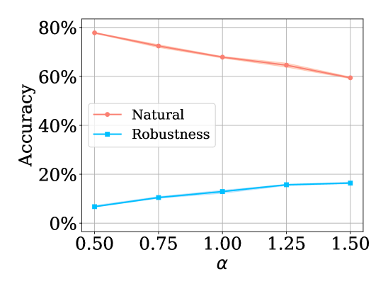
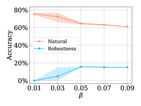
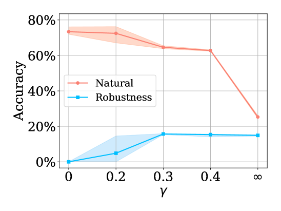
Figure 6: The impact of hyperparameter $\alpha$, $\beta$ and $\gamma$ are shown in the left, middle, and right panels, respectively.

Table 4: Comparison of training cost. The results are obtained on a single NVIDIA RTX 4090 GPU and averaged over 30 training epochs.

Method	FreeAT	Grad Align	ZeroGrad	MultiGrad	V/R/N-FGSM	V/R/N-LAP	PGD-2	PGD-10
Training Time (S)	43.8	36.1	11.1	21.7	11.0	11.8	16.4	59.1

Table 5: Comparison of test accuracy (%) for LAP with various optimization objectives. The results are averaged over three random seeds and reported with the standard deviation.

Method	Natural	Auto Attack
LAP	64.83$\pm$0.29	15.69$\pm$0.28
Original AWP	88.47$\pm$0.75	0.00$\pm$0.00
Modified AWP	30.00$\pm$0.25	12.53$\pm$0.98
LAP-A	59.09$\pm$0.85	15.72$\pm$0.01
LAP-R	53.87$\pm$0.14	11.22$\pm$0.10
LAP-$L_{\infty}$	20.38$\pm$0.38	13.67$\pm$0.35

4.3 Ablation Study

In this part, we conduct an examination of each component within the R-LAP on CIFAR-10 under 16/255 noise magnitude using PreActResNet-18.

Loss Landscape.  To showcase the effectiveness of our proposed method, we illustrate the loss landscape for both the whole model and individual layers, using the same visualization approach as detailed in Section 3.1. Compared to the baseline illustrated in Figure 2, it clearly demonstrates that LAP leads to a more flattened loss landscape for both individual layers and the whole model, as shown in Figure 5. This outcome indicates that our proposed method can effectively hinder the generation of pseudo-robust shortcuts which typically result in sharp decision boundaries, thereby successfully preventing the occurrence of CO.

Optimization Objectives.  We also explore LAP in conjunction with other optimization objectives. These include the Original AWP as defined in Equation 3, Modified AWP retaining the accumulated weight perturbation, LAP-A requiring an Additional backward propagation as outlined in Equation 4, LAP-R plugging the Random weight perturbation, and LAP-$L_{\infty}$ using $L_{\infty}$-norm weight perturbation. To ensure a fair comparison, we conduct a thorough search on the hyperparameter $\beta$ of these methods, and the results are summarized in table 5. It is evident that the original AWP is ineffective at mitigating CO due to its inability to disrupt persistent shortcuts. While the modified AWP can mitigate CO, it demonstrates unsatisfactory natural and robust accuracy. This subpar outcome can be attributed to the introduction of redundant adversarial perturbations in the latter layers, which negatively affect the representation learning. Notably, the LAP-family methods, utilizing diverse operations, can effectively obstruct the generation of pseudo-robust shortcuts, thereby preventing CO. This comprehensive outcome further verifies our perspective that the model’s dependence on these shortcuts triggers the occurrence of CO. Nevertheless, while LAP-A shows a slight improvement in robustness, its requests additional backward propagation that significantly limits its applicability. Meanwhile, LAP-R and LAP-$L_{\infty}$ fail to achieve a comparable performance to the reported LAP implementation.

Hyperparameters Selection.  We separately explore the effects of $\alpha$, $\beta$, and $\gamma$ on both natural and robust accuracy. When tuning one hyperparameter, the others remain fixed. From Figure 6 (left), we can observe that an increase in $\alpha$ leads to improved robust accuracy, but in turn results in a decline in natural accuracy. In light of this trade-off, we follow the original setting and choose not to modify $\alpha$. From the observations in Figure 6 (middle), we note that when $\beta$ is set to a small value, the weight perturbation is inadequate to effectively obstruct pseudo-robust shortcuts and mitigate CO. However, excessively increasing $\beta$ will cause an over-smoothing model, thereby leading to a decrease in natural accuracy. In Figure 6 (right), a similar trend is observed in the adjustment of $\gamma$. When weight perturbation is applied solely to the 1st layer, it fails to effectively hinder the formation of shortcuts. On the other hand, employing uniform weight perturbation across all layers results in a substantial reduction in the natural accuracy.

4.4 Training Cost Analysis

Efficiency is the primary advantage of single-step AT over multi-step AT, offering better scalability to large networks and datasets. Consequently, the computational overhead becomes a crucial factor in assessing the overall performance. In Table 4, we present a comparison of training time consumption among various methods. It is evident that the training cost of the LAP method is comparable to that of the FGSM method, which imposes only a 7% additional training cost. In contrast, the Grad Align and PGD-10 methods are significantly more time-consuming, being 3 and 5 times slower than our method, respectively.

5 Conclusion

In this paper, we reveal that deep neural networks’ dependency on pseudo-robust shortcuts for decision-making triggers the occurrence of catastrophic overfitting. More specifically, our investigation demonstrates the distinct transformation occurring in different network layers, with the former layers experiencing earlier and more severe distortion while the latter layers exhibit relative insensitivity. Our study further discovers that this heightened sensitivity can be attributed to the generation of pseudo-robust shortcuts, which alone can accurately defend against single-step adversarial attacks but bypass genuine-robust learning, leading to distorted decision boundaries. The model exclusively depends on these shortcuts for decision-making inducing the performance paradox. To this end, we introduce an effective and efficient approach, Layer-Aware Adversarial Weight Perturbation (LAP), which strategically applies adaptive perturbations across different layers to hinder the generation of shortcuts, thereby preventing catastrophic overfitting.

Impact Statement

This paper presents work whose goal is to advance the field of adversarial robustness in machine learning. Although single-step adversarial training is the most promising time-efficient method for defending against adversarial examples, it is severely hampered by the catastrophic overfitting problem. In this work, we propose the Layer-Aware Adversarial Weight Perturbation (LAP) method, which aims to effectively and efficiently prevent catastrophic overfitting. Despite LAP being designed to save computing resources, it may still have potential negative impacts on environmental protection (e.g., carbon footprint and global warming). Last and most importantly, while our goal is to develop more secure and robust machine learning for real-world applications, it is crucial to acknowledge that attaining completely safe and trustworthy models is still a distant objective.

Appendix A Experiment with WideResNet and Vit Architecture

WideResNet-34.

To further validate the effectiveness of LAP, we conduct a performance comparison using WideResNet-34 (Zagoruyko & Komodakis, 2016), which is more complex than PreActResNet-18. In the case of WideResNet-34, we adjust the $\beta$ values for the V/R/N-LAP methods to 0.04, 0.024, and 0.005, respectively, while maintaining other hyperparameters consistent with the original configurations.

Table 6: Comparison of WideResNet-34 test accuracy (%) for various methods under 8/255 noise magnitudes on CIFAR-10. The results are averaged over three random seeds and reported with the standard deviation.

Method	V-FGSM	V-LAP	R-FGSM	R-LAP	N-FGSM	N-LAP	PGD-2
Natural	86.10$\pm$1.61	81.92$\pm$1.14	85.21$\pm$0.78	86.10$\pm$0.08	84.85$\pm$0.25	84.42$\pm$0.49	88.55$\pm$0.11
PGD-50-10	0.00$\pm$0.00	44.64$\pm$0.59	0.00$\pm$0.00	46.29$\pm$0.69	49.32$\pm$0.32	50.53$\pm$0.14	46.75$\pm$0.11

Table 6 illustrates that our proposed method, LAP, can consistently prevent CO and achieve a higher level of robustness, comparable to multi-step AT. Moreover, it is worth noting that the complex networks can more significantly demonstrate the efficiency advantages of our method in terms of training time. The results obtained with WideResNet-34 emphasize the applicability of our method in complex network architectures.

Vit-small.

By testing our method on both PreActResNet-18 and WideResNet-34, we have verified its effectiveness in mitigating CO on CNN-based architectures. To further substantiate our perspective and approach, we extend our verification to Transformer-based architectures, specifically Vit-small (Dosovitskiy et al., 2020). Regarding Vit, the $\beta$ settings are detailed in Table 7, with all other hyperparameters remaining in the original setting.

Table 7: Hyperparameter $\beta$ settings for Vit-small.

$\beta$	8/255	12/255	16/255	32/355
V-LAP	0.003	0.006	0.009	0.05
R-LAP	0.002	0.004	0.006	0.04
N-LAP	0.001	0.002	0.003	0.03

Table 8: Comparison of Vit-small test accuracy (%) for various methods under different noise magnitudes on CIFAR-10. The results are averaged over three random seeds and reported with the standard deviation.

Method	8/255			12/255			16/255			32/255
	Natural	PGD-50-10		Natural	PGD-50-10		Natural	PGD-50-10		Natural	PGD-50-10
V-FGSM	39.32$\pm$1.48	25.68$\pm$0.53		25.26$\pm$0.80	17.82$\pm$0.53		14.34$\pm$6.43	0.00$\pm$0.00		12.68$\pm$4.28	0.00$\pm$0.00
V-LAP	41.98$\pm$0.61	26.38$\pm$0.14		24.53$\pm$0.45	18.18$\pm$0.62		17.85$\pm$0.62	11.79$\pm$0.24		16.44$\pm$0.14	8.93$\pm$0.13
R-FGSM	45.08$\pm$0.37	26.28$\pm$0.30		28.08$\pm$0.99	18.80$\pm$0.38		23.80$\pm$1.07	14.27$\pm$0.04		13.71$\pm$2.11	0.00$\pm$0.00
R-LAP	46.56$\pm$0.03	27.06$\pm$0.42		27.60$\pm$0.49	19.01$\pm$0.24		21.72$\pm$0.14	15.49$\pm$0.24		17.15$\pm$0.78	9.04$\pm$0.21
N-FGSM	37.30$\pm$1.98	24.84$\pm$0.74		24.85$\pm$0.97	17.61$\pm$0.45		20.68$\pm$0.80	13.38$\pm$1.93		8.67$\pm$1.89	0.00$\pm$0.00
N-LAP	40.48$\pm$0.56	25.69$\pm$0.29		24.15$\pm$0.65	17.99$\pm$0.67		20.19$\pm$0.80	14.15$\pm$0.26		15.75$\pm$0.35	8.49$\pm$0.50
PGD-2	48.97$\pm$0.41	26.21$\pm$0.42		32.25$\pm$0.83	19.51$\pm$0.28		25.42$\pm$1.00	16.04$\pm$0.19		18.04$\pm$3.97	9.67$\pm$3.79

It is worth emphasizing that prior research has identified that the CO phenomenon also exists in the Vit model (Shao et al., 2022), consistent with our observations in Table 8. Furthermore, the above results underscore two significant differences in the baseline performance between CNN-based and Transformer-based architectures. Firstly, Vit exhibits a lower susceptibility to CO, showing that the V-FGSM does not experience CO when the noise magnitudes are 8 and 12/255, and the R-FGSM can also be effectively trained when the noise magnitude is 16/255. Secondly, the R-FGSM attains the most excellent outcome in baselines, which could be attributed to the larger perturbation introduced by the N-FGSM that disrupts the Transformer-based model learning. Most importantly, Table 8 highlights that our approach can effectively mitigate CO and improve robust accuracy across all levels of noise magnitudes. It is evident both the universality of our perspective and the effectiveness of our approach when applied to Transformer-based architectures.

Appendix B Settings and Results on Tiny-ImageNet Dataset

We also extend our method to a large-sized dataset, Tiny-ImageNet (Netzer et al., 2011), to showcase its effectiveness. In the case of Tiny-ImageNet, we set the $\beta$ values for the V/R/N-LAP methods to 0.016, 0.006, and 0.002, while keeping other hyperparameters consistent with their original configurations.

Table 9: Comparison of Tiny-imagenet test accuracy (%) for various methods under 8/255 noise magnitudes using PreactResNet-18. The results are averaged over three random seeds and reported with the standard deviation.

Method	V-FGSM	V-LAP	R-FGSM	R-LAP	N-FGSM	N-LAP	PGD-2
Natural	32.70$\pm$4.55	47.35$\pm$0.46	51.65$\pm$2.15	50.05$\pm$0.47	48.86$\pm$0.75	47.82$\pm$0.24	46.58$\pm$0.45
PGD-50-10	0.00$\pm$0.00	17.64$\pm$0.61	0.00$\pm$0.00	19.03$\pm$0.18	20.58$\pm$0.49	20.82$\pm$0.20	20.42$\pm$0.39

Table 9 presents the results of LAP applied to the Tiny-ImageNet dataset. These results again substantiate our approach’s efficacy in effectively preventing CO and enhancing robust accuracy, establishing it as a dependable solution for large-scale datasets.

Appendix C Long Training Schedule Results

We have further evaluated the performance of our method using the standard multi-step AT schedule (Rice et al., 2020), which consists of 200 epochs with an initial learning rate of 0.1. The learning rate is reduced by 10 at the 100th and 150th epochs, respectively.

Table 10: Comparison of long training schedule test accuracy (%) for various methods under 8/255 noise magnitudes using PreactResNet-18. The results are averaged over three random seeds and reported with the standard deviation.

Method	V-FGSM	V-LAP	R-FGSM	R-LAP	N-FGSM	N-LAP	PGD-2
Natural	87.94$\pm$0.35	80.11$\pm$0.18	90.89$\pm$0.76	85.09$\pm$0.85	83.55$\pm$0.14	83.15$\pm$0.20	86.53$\pm$0.25
PGD-50-10	0.00$\pm$0.00	31.26$\pm$0.10	0.00$\pm$0.00	36.17$\pm$0.53	36.79$\pm$0.38	37.37$\pm$0.21	37.99$\pm$0.07

Table 10 illustrates that our method, LAP, consistently enhances adversarial robustness in the face of another commonly adopted training schedule. This reaffirms the LAP’s consistent, reliable, and effective performance in mitigating CO.

References

- Andriushchenko & Flammarion (2020) Andriushchenko, M. and Flammarion, N. Understanding and improving fast adversarial training. Advances in Neural Information Processing Systems, 33:16048–16059, 2020.
- Athalye et al. (2018) Athalye, A., Carlini, N., and Wagner, D. Obfuscated gradients give a false sense of security: Circumventing defenses to adversarial examples. In International conference on machine learning, pp. 274–283. PMLR, 2018.
- Croce & Hein (2020) Croce, F. and Hein, M. Reliable evaluation of adversarial robustness with an ensemble of diverse parameter-free attacks. In International conference on machine learning, pp. 2206–2216. PMLR, 2020.
- Croce et al. (2022) Croce, F., Gowal, S., Brunner, T., Shelhamer, E., Hein, M., and Cemgil, T. Evaluating the adversarial robustness of adaptive test-time defenses. In International Conference on Machine Learning, pp. 4421–4435. PMLR, 2022.
- de Jorge Aranda et al. (2022) de Jorge Aranda, P., Bibi, A., Volpi, R., Sanyal, A., Torr, P., Rogez, G., and Dokania, P. Make some noise: Reliable and efficient single-step adversarial training. Advances in Neural Information Processing Systems, 35:12881–12893, 2022.
- Dong et al. (2023) Dong, Y., Liu, C., Xiang, W., Su, H., and Zhu, J. Competition on robust deep learning. National Science Review, 10(6):nwad087, 2023.
- Dosovitskiy et al. (2020) Dosovitskiy, A., Beyer, L., Kolesnikov, A., Weissenborn, D., Zhai, X., Unterthiner, T., Dehghani, M., Minderer, M., Heigold, G., Gelly, S., et al. An image is worth 16x16 words: Transformers for image recognition at scale. In International Conference on Learning Representations, 2020.
- Dziugaite & Roy (2017) Dziugaite, G. K. and Roy, D. M. Computing nonvacuous generalization bounds for deep (stochastic) neural networks with many more parameters than training data. arXiv preprint arXiv:1703.11008, 2017.
- Foret et al. (2020) Foret, P., Kleiner, A., Mobahi, H., and Neyshabur, B. Sharpness-aware minimization for efficiently improving generalization. In International Conference on Learning Representations, 2020.
- Golgooni et al. (2023) Golgooni, Z., Saberi, M., Eskandar, M., and Rohban, M. H. Zerograd: Costless conscious remedies for catastrophic overfitting in the fgsm adversarial training. Intelligent Systems with Applications, 19:200258, 2023.
- Goodfellow et al. (2014) Goodfellow, I. J., Shlens, J., and Szegedy, C. Explaining and harnessing adversarial examples. arXiv preprint arXiv:1412.6572, 2014.
- He et al. (2016) He, K., Zhang, X., Ren, S., and Sun, J. Identity mappings in deep residual networks. In European conference on computer vision, pp. 630–645. Springer, 2016.
- He et al. (2019) He, Z., Rakin, A. S., and Fan, D. Parametric noise injection: Trainable randomness to improve deep neural network robustness against adversarial attack. In Proceedings of the IEEE/CVF Conference on Computer Vision and Pattern Recognition, pp. 588–597, 2019.
- Huang et al. (2023a) Huang, Z., Fan, Y., Liu, C., Zhang, W., Zhang, Y., Salzmann, M., Süsstrunk, S., and Wang, J. Fast adversarial training with adaptive step size. IEEE Transactions on Image Processing, 2023a.
- Huang et al. (2023b) Huang, Z., Zhu, M., Xia, X., Shen, L., Yu, J., Gong, C., Han, B., Du, B., and Liu, T. Robust generalization against photon-limited corruptions via worst-case sharpness minimization. In Proceedings of the IEEE/CVF Conference on Computer Vision and Pattern Recognition, pp. 16175–16185, 2023b.
- Keskar et al. (2016) Keskar, N. S., Mudigere, D., Nocedal, J., Smelyanskiy, M., and Tang, P. T. P. On large-batch training for deep learning: Generalization gap and sharp minima. In International Conference on Learning Representations, 2016.
- Kim et al. (2021) Kim, H., Lee, W., and Lee, J. Understanding catastrophic overfitting in single-step adversarial training. In Proceedings of the AAAI Conference on Artificial Intelligence, volume 35, pp. 8119–8127, 2021.
- Krizhevsky et al. (2009) Krizhevsky, A., Hinton, G., et al. Learning multiple layers of features from tiny images. 2009.
- Li & Spratling (2023) Li, L. and Spratling, M. Understanding and combating robust overfitting via input loss landscape analysis and regularization. Pattern Recognition, 136:109229, 2023.
- Li et al. (2022) Li, T., Wu, Y., Chen, S., Fang, K., and Huang, X. Subspace adversarial training. In Proceedings of the IEEE/CVF Conference on Computer Vision and Pattern Recognition, pp. 13409–13418, 2022.
- Lin et al. (2023a) Lin, R., Yu, C., Han, B., and Liu, T. On the over-memorization during natural, robust and catastrophic overfitting. In The Twelfth International Conference on Learning Representations, 2023a.
- Lin et al. (2023b) Lin, R., Yu, C., and Liu, T. Eliminating catastrophic overfitting via abnormal adversarial examples regularization. In Thirty-seventh Conference on Neural Information Processing Systems, 2023b.
- Madry et al. (2018) Madry, A., Makelov, A., Schmidt, L., Tsipras, D., and Vladu, A. Towards deep learning models resistant to adversarial attacks. In International Conference on Learning Representations, 2018.
- Netzer et al. (2011) Netzer, Y., Wang, T., Coates, A., Bissacco, A., Wu, B., and Ng, A. Y. Reading digits in natural images with unsupervised feature learning. 2011.
- Neyshabur et al. (2017) Neyshabur, B., Bhojanapalli, S., McAllester, D., and Srebro, N. Exploring generalization in deep learning. Advances in neural information processing systems, 30, 2017.
- Niu et al. (2022) Niu, A., Zhang, K., Zhang, C., Zhang, C., Kweon, I. S., Yoo, C. D., and Zhang, Y. Fast adversarial training with noise augmentation: A unified perspective on randstart and gradalign. arXiv preprint arXiv:2202.05488, 2022.
- Park & Lee (2021) Park, G. Y. and Lee, S. W. Reliably fast adversarial training via latent adversarial perturbation. In Proceedings of the IEEE/CVF International Conference on Computer Vision, pp. 7758–7767, 2021.
- Rice et al. (2020) Rice, L., Wong, E., and Kolter, Z. Overfitting in adversarially robust deep learning. In International Conference on Machine Learning, pp. 8093–8104. PMLR, 2020.
- Rocamora et al. (2023) Rocamora, E. A., Liu, F., Chrysos, G., Olmos, P. M., and Cevher, V. Efficient local linearity regularization to overcome catastrophic overfitting. In The Twelfth International Conference on Learning Representations, 2023.
- Shafahi et al. (2019) Shafahi, A., Najibi, M., Ghiasi, M. A., Xu, Z., Dickerson, J., Studer, C., Davis, L. S., Taylor, G., and Goldstein, T. Adversarial training for free! Advances in Neural Information Processing Systems, 32, 2019.
- Shao et al. (2022) Shao, R., Shi, Z., Yi, J., Chen, P.-Y., and Hsieh, C.-J. On the adversarial robustness of vision transformers. Transactions on Machine Learning Research, 2022.
- Smith (2017) Smith, L. N. Cyclical learning rates for training neural networks. In 2017 IEEE winter conference on applications of computer vision (WACV), pp. 464–472. IEEE, 2017.
- Sriramanan et al. (2021) Sriramanan, G., Addepalli, S., Baburaj, A., et al. Towards efficient and effective adversarial training. Advances in Neural Information Processing Systems, 34:11821–11833, 2021.
- Vivek & Babu (2020) Vivek, B. and Babu, R. V. Single-step adversarial training with dropout scheduling. In 2020 IEEE/CVF Conference on Computer Vision and Pattern Recognition (CVPR), pp. 947–956. IEEE, 2020.
- Wang et al. (2024) Wang, Y., Li, L., Yang, J., Lin, Z., and Wang, Y. Balance, imbalance, and rebalance: Understanding robust overfitting from a minimax game perspective. Advances in neural information processing systems, 36, 2024.
- Wen et al. (2018) Wen, Y., Vicol, P., Ba, J., Tran, D., and Grosse, R. Flipout: Efficient pseudo-independent weight perturbations on mini-batches. In International Conference on Learning Representations, 2018.
- Wong et al. (2019) Wong, E., Rice, L., and Kolter, J. Z. Fast is better than free: Revisiting adversarial training. In International Conference on Learning Representations, 2019.
- Wu et al. (2020) Wu, D., Xia, S.-T., and Wang, Y. Adversarial weight perturbation helps robust generalization. Advances in Neural Information Processing Systems, 33:2958–2969, 2020.
- Yu et al. (2022a) Yu, C., Han, B., Gong, M., Shen, L., Ge, S., Du, B., and Liu, T. Robust weight perturbation for adversarial training. In The Thirty-First International Joint Conference on Artificial Intelligence, 2022a.
- Yu et al. (2022b) Yu, C., Han, B., Shen, L., Yu, J., Gong, C., Gong, M., and Liu, T. Understanding robust overfitting of adversarial training and beyond. In International Conference on Machine Learning, pp. 25595–25610. PMLR, 2022b.
- Zagoruyko & Komodakis (2016) Zagoruyko, S. and Komodakis, N. Wide residual networks. In Procedings of the British Machine Vision Conference 2016. British Machine Vision Association, 2016.
- Zhang et al. (2019) Zhang, H., Yu, Y., Jiao, J., Xing, E., El Ghaoui, L., and Jordan, M. Theoretically principled trade-off between robustness and accuracy. In International conference on machine learning, pp. 7472–7482. PMLR, 2019.
- Zhou et al. (2022) Zhou, D., Wang, N., Han, B., and Liu, T. Modeling adversarial noise for adversarial training. In International Conference on Machine Learning, pp. 27353–27366. PMLR, 2022.