USD: Unsupervised Soft Contrastive Learning for Fault Detection in Multivariate Time Series
Abstract
Unsupervised fault detection in multivariate time series is critical for maintaining the integrity and efficiency of complex systems, with current methodologies largely focusing on statistical and machine learning techniques. However, these approaches often rest on the assumption that data distributions conform to Gaussian models, overlooking the diversity of patterns that can manifest in both normal and abnormal states, thereby diminishing discriminative performance. Our innovation addresses this limitation by introducing a combination of data augmentation and soft contrastive learning, specifically designed to capture the multifaceted nature of state behaviors more accurately. The data augmentation process enriches the dataset with varied representations of normal states, while soft contrastive learning fine-tunes the model’s sensitivity to the subtle differences between normal and abnormal patterns, enabling it to recognize a broader spectrum of anomalies. This dual strategy significantly boosts the model’s ability to distinguish between normal and abnormal states, leading to a marked improvement in fault detection performance across multiple datasets and settings, thereby setting a new benchmark for unsupervised fault detection in complex systems. The code of our method is available at https://github.com/zangzelin/code_USD.git.
I Introduction
In the realm of industrial operations and complex systems management [25], unsupervised fault detection [33] in multivariate time series data holds paramount importance. This technology underpins the early identification of potential failures and anomalies, safeguarding against costly downtimes and ensuring the continuity of critical processes [15]. Current methodologies in this field span a broad spectrum, from traditional statistical approaches to advanced machine learning models, each aiming to autonomously detect irregularities without the need for labeled data [32, 27]. These techniques are crucial in environments where supervisory labels are scarce or infeasible to obtain, making unsupervised methods invaluable for real-time monitoring and preventive maintenance strategies [35].
However, despite the use of deep learning [18] mathods advanced unsupervised fault detection techniques, false alarms and missed alarms are still common in practice (as shown in Table. II). The main problem stems from the unsupervised approach itself, which avoids the laborious task of manually collecting labels, but also loses the ability to precisely define different states. Without explicit labels, the system must rely on certain assumptions to distinguish between normal and abnormal states. As a result, as shown in Fig. 1(a), many existing methods use the Gaussian assumption that abnormal states are outliers in a Gaussian distribution. While this simplifies the modeling process, it fails to capture the complexity and diversity of the actual operating states, which weakens the ability to accurately detect subtle differences between states and reduces the effectiveness of fault detection models.
Theoretically, as shown in Fig. 1(b), the Gaussian assumption ignores the fact that both normal and abnormal states may contain multiple sub-states. This lead to unnatural distortions in the shape of the data stream, which ultimately affects the performance of these methods. Practically speaking, the Gaussian assumption simplifies the modeling process but does not take into account the inherent complexity and diversity of patterns that characterize the operating state. This simplification reduces the discriminative power of fault detection models, masking subtle differences and transitions between normal operation and potential faults.
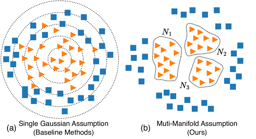
To address the above issues, we introduce an unsupervised soft contrast learning framework, named Unsupervised Soft Fault Detection (USD), to go beyond the limitations imposed by the Gaussian distribution assumption by using more accurate multi-Gaussian representations [34]. As shown in Fig. 1(b), we first design a neighbor-based unsupervised data augmentation method to generate positive samples for unsupervised contrast learning [16] through online data augmentation of multivariate time series data. Then, we compute the loss function for soft contrast learning by incorporating a representation learning head module. Soft contrast learning optimizes the discriminative representation space based on the similarity of local streamforms to better portray the difference between normal and abnormal states. We argue that incorporating soft contrast learning not only enhances the model’s ability to distinguish between normal and abnormal patterns, but also captures a wider range of potential anomalies [37]; thus providing a more accurate, robust and adaptive solution.
Experimental evaluations show that our model performance (AUC and PR) is significantly improved compared to existing fault detection frameworks. Specifically, our approach achieves new enhancements on multiple standard test benchmarks (SWaT [9], WADI [2]) and operational scenarios with lower false alarm rates and higher detection accuracies. At the same time, we demonstrate, e.g., through visualization, the plausibility of our multi-Gaussian assumptions and the fact that soft-contrast learning can characterize different sub-states well. We summarize the contributions of this paper as follows.
-
•
Proposes a more plausible assumption of multiple manifold. In this paper, by challenging the traditional reliance on Gaussian distribution assumptions, our approach recognizes and accommodates the existence of many different states under normal and abnormal operating conditions. This realization of the complexity of the state space is critical to the development of more detailed and effective fault detection systems.
-
•
Introduces a soft contrast learning framework for performing latent space representations. We introduce a novel combination of data augmentation and soft contrastive learning techniques to represent these diverse states accurately. This methodology not only enhances the precision of state representations but also ensures that the subtle differences and transitions between normal and abnormal conditions are captured more effectively.
-
•
Obtain a significant performance boost. The practical efficacy of our approach is demonstrated through significant performance improvements across multiple datasets, with our model outperforming existing benchmarks by over 5%. These advancements underscore our contributions towards developing a more adaptive, accurate, and robust framework for unsupervised fault detection, paving the way for future innovations in monitoring and maintaining complex systems.
II Related Work
II-A Time Series Anomaly Detection
In the evolving landscape of time series anomaly detection, the reliance on One-Class Classification (OCC) based methods, such as those presented by Chalapathy and Chawla [5], Hundman et al. [13], and further exemplified by DeepSVDD [22], EncDecAD [20], OmniAnomaly [24], USAD [4], and DAEMON [7], has underscored a critical limitation in their operational premise. These methods, by design, necessitate a training dataset composed entirely of normal instances, a requirement that is not only challenging but often impractical in real-world scenarios. The presence of even a small fraction of anomalous data within the training set can significantly impair the model’s detection capabilities, as highlighted by Wang et al. [26] and Huyan et al. [14]. This recognition of inherent limitations has spurred the exploration of alternative approaches that can circumvent the constraints imposed by OCC-based frameworks.
Responding to this challenge, Dai and Chen introduced GANF [8], a pioneering method that adopts an unsupervised learning strategy for the detection of Multivariate Time Series (MTS) anomalies. Qihang Zhou introduced MTGFlow [34], an unsupervised anomaly detection approach for Multivariate Time Series, leveraging dynamic graph structures and entity-aware normalizing flows for density estimation. The method notably incorporates MTGFlow-cluster [35], a strategy that clusters entities with similar characteristics to enhance precision, achieving superior performance on benchmark datasets. Chen Liu [19] proposed AnomalyLLM, a knowledge distillation-based time series anomaly detection method utilizing a large language model (LLM) as a teacher to guide a student network. Incorporating prototypical signals and synthetic anomalies, AnomalyLLM significantly improves detection accuracy by at least 14.5% on the UCR dataset, showcasing its effectiveness across 15 datasets.
II-B Contrastive Learning and Soft Contrastive Learning
Soft contrastive learning [31, 29] and deep manifold learning [21, 17] represent two advanced methodologies in the domain of machine learning, particularly in the tasks of unsupervised learning and representation learning. These techniques aim to leverage the intrinsic structure of the data to learn meaningful and discriminative features.
At its core, soft contrastive learning [31, 29] is an extension of the contrastive learning framework [6, 11, 12], which aims to learn representations by bringing similar samples closer and pushing dissimilar samples apart in the representation space. However, soft contrastive learning introduces a more nuanced approach by incorporating the degrees of similarity between samples into the learning process, rather than treating similarity as a binary concept. This is achieved through the use of soft labels or continuous similarity scores, allowing the model to learn richer and more flexible representations. The softness in the approach accounts for the varying degrees of relevance or similarity among data points, making it particularly useful in tasks where the relationship between samples is not strictly binary or categorical, such as in semi-supervised learning or in scenarios with noisy labels.
III Preliminary
In this section, we give a brief introduction of normalizing flow based false detection to better understand our proposed USD.
Normalizing flow is an unsupervised density estimation approach to map the original distribution to an arbitrary target distribution by the stack of invertible affine transformations. When density estimation on original data distribution is intractable, an alternative option is to estimate density on target distribution . Specifically, suppose a source sample and a target distribution sample . Bijective invertible transformation aims to achieve one-to-one mapping from to . According to the change of variable formula, we can get
| (1) |
Benefiting from the invertibility of mapping functions and tractable jacobian determinants . The objective of flow models is to achieve , where .
Flow models are able to achieve more superior density estimation performance when additional conditions are input [3]. Such a flow model is called conditional normalizing flow, and its corresponding mapping is derived as . Parameters of are updated by maximum likelihood estimation (MLE):
| (2) |
IV Methodology
IV-A Notation and Problem Definition
Consider a multivariate time series (MTS) data set . The data set encompassing entities, each with observations, and denotes as , where each . Z-score normalization is employed to standardize the time series data across different entities. A sliding window approach, with a window size of and a stride size of , is utilized to sample the normalized MTS, generating training samples , where denotes the sampling count, and represents the segment .
The objective of unsupervised fault detection is to identify segments within exhibiting anomalous behavior. This process operates under the premise that the normal behavior of is known, and any significant deviation from this behavior is considered abnormal. Specifically, abnormal behavior is characterized by its occurrence in low-density regions of the normal behavior distribution, defined by a density threshold . The task of unsupervised fault detection in MTS can thus be formalized as identifying segments where .
Definition 1 (Supervised Fault Detection in MTS).
Let be a labeled dataset for an MTS, where each segment is annotated with a label , indicating normal () or abnormal () behavior. Supervised fault detection aims to learn a function that can accurately classify new, unseen segments as normal or abnormal based on learned patterns of faults.
Definition 2 (Unsupervised Fault Detection under Gaussian Assumption).
In the Gaussian assumption context, unsupervised fault detection in an MTS operates on the premise that the distribution of normal behavior can be modeled using a Gaussian distribution. Anomalies are identified as segments that fall in regions of low probability under this Gaussian model, specifically where , with being a predefined density threshold.
Definition 3 (Unsupervised Fault Detection under Multi-Gaussian Assumption).
Under the multi-Gaussian assumption, unsupervised fault detection recognizes that the distribution of normal behavior in an MTS may encompass multiple modes, each fitting a Gaussian model. This assumption allows for a more nuanced detection of anomalies, which are segments that do not conform to any of the modeled Gaussian distributions of normal behavior, detected through a composite density threshold criterion .
IV-B Neural Network Structure of USD
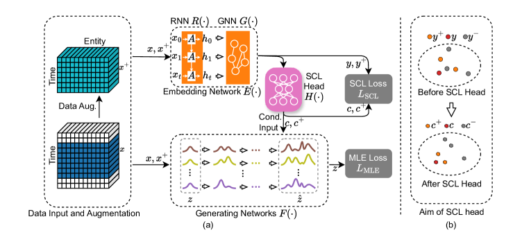
The core idea of USD is to learn more accurate latent spatial representations using a combination of data augmentation and soft contrast learning. Fig. 2 illustrates the details of USD framework, which synergizes RNN , GNN , and FLOW model to adeptly navigate the complexities of multivariate time series data for fault detection. In summary, the RNN captures the temporal correlations within the data, generating time encodings that are then input into the GNN to capture the dynamic interdependencies among entities. The output of the GNN , representing the spatio-temporal conditions of the entities, is fed into the entity-aware normalizing flow model for density estimation, enabling the model to discern normal and abnormal states with precision. The specific detailed definitions are as follows:
Temporal Dynamics with RNN []. We model the temporal variations of each entity using an RNN . The hidden state at time window is updated as
| (3) |
where represents the input features at time window , the is the parameter of RNN, and is the hidden state of the RNN at time window .
Dynamic Interdependencies with GNN []. A graph structure learning module captures the dynamic interdependencies among entities. The graph convolution operation, applied to the time encoding from the RNN and the learned graph structure , is given by
| (4) |
where represents the spatio-temporal condition of the entities at time window , is the parameter of GNN, and is the output of the GNN at time window . The graph structure learning module captures the evolving interdependencies among entities, enabling the model to discern the complex relationships and interactions that underpin the multivariate time series data.
Soft Contrastive Learning Head with MLP []. To refine the feature representations and enhance the discriminative power of the model, a Soft Contrastive Learning Head implemented with a Multilayer Perceptron (MLP) is employed. This component takes the output from the GNN as input and processes it to generate a transformed feature space where similar samples are brought closer, and dissimilar samples are pushed apart. The transformation is defined as:
| (5) |
where represents the contrastively learned feature representation of the entities at time window , and denotes the parameters of the MLP. The objective of this component is to maximize the margin between different classes in the feature space, effectively improving the separability and robustness of the model. This is achieved through a contrastive loss function, which penalizes similar pairs that are too far apart and dissimilar pairs that are too close, thereby fine-tuning the embeddings to better capture the nuances of the underlying data dynamics.
Density Estimation with FLOW Model []. The spatio-temporal conditions are then input into the entity-aware normalizing flow model for fine-grained density estimation. The transformation of a data point into through the flow model is described as
| (6) |
where represents the flow transformation parameterized by .
IV-C Maximum Likelihood Estimation (MLE) Loss
To enhance the anomaly detection capabilities of the USD framework, which includes the RNN, GNN, and FLOW models, the entire system is optimized using Maximum Likelihood Estimation (MLE). This optimization approach ensures the models are finely tuned to detect anomalies effectively:
| (7) |
where represents the total number of time windows, denotes the number of entities, and is the mean vector of the target distribution . The MLE loss function is crafted to maximize the probability of the transformed data points being observed under the model’s assumptions, thereby ensuring that the model faithfully represents the true distribution of the data.
IV-D Data Augmentation for Soft Contrastive Learning
Data augmentation is crucial for improving the model’s ability to generalize beyond the training data by artificially expanding the dataset’s size and diversity [30]. Our methodology incorporates two primary strategies: neighborhood discovery and linear interpolation.
Neighborhood Discovery. This technique focuses on leveraging the local structure of the data to generate new, plausible data points that conform to the existing distribution. For each data point , we define its neighborhood using a distance metric , such as the Euclidean distance. The neighborhood consists of points that meet the criterion:
| (8) |
where is a predetermined threshold defining the neighborhood’s radius. This method captures the local density of the data, enabling the generation of new samples within these densely populated areas and thus enhancing the dataset with variations that align with the original data distribution.
Data Augmentation by Linear Interpolation. Data augmentation strategy augments the dataset by creating intermediate samples between existing data points [28]. For two points and , a new sample is formulated as:
| (9) |
where is a random coefficient sampled from a uniform distribution, . This approach facilitates a smooth transition between data points, effectively bridging gaps in the data space and introducing a continuum of sample variations. By interpolating between points either within the same neighborhood or across different neighborhoods, we substantially enhance the dataset’s diversity and coverage, providing the model with a more comprehensive set of examples for training.
Together, neighborhood discovery and linear interpolation form a powerful data augmentation framework that leverages both the local structure and the linear relationships within the data. This approach not only expands the dataset but also ensures that the augmented samples are meaningful and representative of the original data characteristics, thereby improving the model’s performance and robustness.
IV-E Soft Contrastive Learning Loss with Data Augmentation
In data-augmentation-based contrastive learning (CL), the task is framed as a binary classification problem over pairs of samples. Positive pairs, drawn from the joint distribution , are labeled as , whereas negative pairs, drawn from the product of marginals , are labeled as . The goal of contrastive learning is to learn representations that maximize the similarity between positive pairs and minimize it between negative pairs, utilizing the InfoNCE loss.
| (10) | ||||
where constitutes a positive pair and a negative pair, with being the embeddings of respectively, and representing the number of negative pairs. The similarity function is typically defined using cosine similarity. This method effectively enhances the model’s discriminative power by distinguishing between closely related (positive) and less related (negative) samples within the augmented data space.
The conventional contrastive learning (CL) loss is structured around a single positive sample contrasted against multiple negatives. To refine this, we have restructured the CL loss into a more nuanced form that utilizes labels for positive and negative samples, denoted by . Detailed explanations of this transformation from Eq. (10) to Eq. (11) are available in Appendix A. Details of SCL loss.
| (11) | ||||
where indicates if samples and have been augmented from the same source. signifies a positive pair , and indicates a negative pair. The term represents the density ratio, as defined and computed by the backbone network.
To mitigate issues arising from view-noise, we introduce Soft Contrastive Learning (SCL). This approach moderates the impact of erroneous sample classifications by variably weighting different samples, calculated through similarity assessments by the network itself. The SCL loss function is defined as:
| (12) | ||||
where represents a softened version of , acting as weights for the samples, and is the density ratio.
| (13) |
where, is a hyper-parameter in the range [0,1], infusing prior knowledge of the data augmentation relationship into model training. The kernel function maps high-dimensional vectors to probability values. For this paper, we employ the t-distribution kernel function due to its flexibility in adjusting the closeness of distribution in dimensionality reduction mappings.
| (14) |
where is the Gamma function, and represents the degrees of freedom, which dictate the kernel’s shape. The SCL loss employs a softer optimization target compared to the rigid structure of traditional CL loss, enhancing resilience against noisy labels. A comprehensive discussion on the differences between these loss functions is provided in Appendix A.3 SCL is better than CL in view-noise, along with proof that SCL maintains a higher signal-to-noise ratio when confronted with view-noise.
IV-F Optimization Objectives
The entire USD framework, encompassing the RNN, GNN, and FLOW models, is optimized jointly through Maximum Likelihood Estimation (MLE) to ensure effective anomaly detection. The joint optimization process is formulated as follows:
| (15) |
where is the MLE loss, and is the SCL loss. The MLE loss is designed to maximize the likelihood of observing the transformed data points under the model, while the SCL loss is designed to enhance the model’s sensitivity to subtle differences between normal and abnormal patterns. By embedding these mathematical formulations into each step of the USD framework, we ensure a rigorous approach to modeling and detecting anomalies in multivariate time series data, setting a new standard for unsupervised fault detection in complex systems.
IV-G Pseudocode
Algorithm. 1 shows how to train our model and how to obtain the selected features.
Input:
Train windows Data: ,
Test windows Data: ,
Learning rate: ,
Epochs: ,
Batch size: ,
Network: ,
loss weights: ,
Output:
, the prediction of USD
Return:
V Experiments
V-A Dataset Information and Implementation Details.
Datasets information. We selected the five most commonly used datasets for fault detection to evaluate the effectiveness of our method. These datasets are widely recognized in the field of One-Class Classification (OCC) for Multivariate Time Series (MTS) anomaly detection. The datasets include:
-
•
SWaT (Secure Water Treatment) [9]: Originating from a scaled-down version of an industrial water treatment plant, the SWaT dataset is used for research in cybersecurity and anomaly detection in critical infrastructure systems. SWaT collects 51 sensor data from a real-world industrial water treatment plant, at the frequency of one second. The dataset provides ground truths of 41 attacks launched during 4 days. 111https://itrust.sutd.edu.sg/itrust-labs_datasets/dataset_info.
-
•
WADI (Water Distribution) [2]: The WADI dataset is collected from a water distribution testbed, simulating real-world water supply networks. It is particularly useful for studying the impact of cyber-attacks on public utility systems. WADI collects 121 sensor and actuators data from WADI testbed, at the frequency of one second. The dataset provides ground truths of 15 attacks launched during 2 days. 222https://itrust.sutd.edu.sg/itrust-labs_datasets/dataset_info/.
-
•
PSM (Pooled Server Metrics) [1]: This dataset aggregates performance metrics from multiple server nodes managed by eBay. It is utilized to identify outliers indicating potential issues in server performance or security breaches 333https://github.com/tuananhphamds/MST-VAE.
-
•
MSL (Mars Science Laboratory rover) [13]: This dataset originates from the Mars Science Laboratory rover, specifically the Curiosity rover. It includes telemetry data used to detect anomalies in the rover’s operational parameters during its mission on Mars 444https://github.com/khundman/telemanom.
-
•
SMD (Server Machine Dataset) [24]: Collected from a large internet company’s server farms, this dataset comprises metrics from different server machines, providing a basis for detecting unusual behaviors in server operations 555https://github.com/NetManAIOps/OmniAnomaly.
Datasets split and preprocessing. In our experimental setup, we adhere to the dataset configurations used in the GANF study [8]. MTGFlow [8] and MTGFlow_Cluster [8]. Specifically, for the SWaT dataset, we partition the original testing data into 60% for training, 20% for validation, and 20% for testing. For the other datasets, the training partition comprises 60% of the data, while the test partition contains the remaining 40%. The training data is used to train the model, while the validation data is used to tune hyperparameters and the test data is used to evaluate the model’s performance. The datasets are preprocessed to remove missing values and normalize the data to a range of [0, 1]. The data is then divided into fixed-length sequences, with a window size of 60 and a stride of 10. The window size determines the number of time steps in each sequence, while the stride determines the step size between each sequence. The data is then fed into the model for training and evaluation.
| Dataset |
|
|
|
|
|
|||||||||||||
|---|---|---|---|---|---|---|---|---|---|---|---|---|---|---|---|---|---|---|
| SWaT | 51 | 269,951 | 89,984 | 17.7 | 5.2 | |||||||||||||
| WADI | 123 | 103,680 | 69,121 | 6.4 | 4.6 | |||||||||||||
| PSM | 25 | 52,704 | 35,137 | 23.1 | 34.6 | |||||||||||||
| MSL | 55 | 44,237 | 29,492 | 14.7 | 4.3 | |||||||||||||
| SMD | 38 | 425,052 | 283,368 | 4.2 | 4.1 |
| Methods | Journal-Year | Area Under the Receiver Operating Characteristic Curve (AUROC) | Average | Rank | ||||
|---|---|---|---|---|---|---|---|---|
| SWaT | WADI | PSM | MSL | SMD | ||||
| DROCC [10] | ICML, 2020 | 72.6(±3.8) | 75.6(±1.6) | 74.3(±2.0) | 53.4(±1.6) | 76.7(±8.7) | 70.5 | 6 |
| DeepSAD [23] | ICLR, 2020 | 75.4(±2.4) | 85.4(±2.7) | 73.2(±3.3) | 61.6(±0.6) | 85.9(±11.1) | 76.3 | 5 |
| USAD [4] | KDD, 2020 | 78.8(±1.0) | 86.1(±0.9) | 78.0(±0.2) | 57.0(±0.1) | 86.9(±11.7) | 77.4 | 4 |
| DAGMM [36] | ICLR, 2018 | 72.8(±3.0) | 77.2(±0.9) | 64.6(±2.6) | 56.5(±2.6) | 78.0(±9.2) | 69.8 | 7 |
| GANF [8] | ICLR, 2022 | 79.8(±0.7) | 90.3(±1.0) | 81.8(±1.5) | 64.5(±1.9) | 89.2(±7.8) | 81.1 | 3 |
| MTGFlow [34] | AAAI, 2023 | 84.8(±1.5) | 91.9(±1.1) | 85.7(±1.5) | 67.2(±1.7) | 91.3(±7.6) | 84.2 | 2 |
| MTGFlow_Cluster [35] | TKDE, 2024 | 83.1(±1.3) | 91.8(±0.4) | 87.1(±2.4) | 68.2(±2.6) | - | - | - |
| USD | OURS | 90.2(±0.9) | 94.1(±0.4) | 88.9(±2.4) | 74.2(±2.0) | 94.2(±6.5) | 88.3 | 1 |
| USD* | OURS | 92.0(±1.2) | 94.9(±1.2) | 88.9(±2.4) | 76.0(±1.1) | 94.2(±6.5) | 89.2 | 1* |
| Methods | Journal-Year | Area Under the Precision-Recall Curve (AUPRC) | Average | Rank | ||||
|---|---|---|---|---|---|---|---|---|
| SWaT | WADI | PSM | MSL | SMD | ||||
| DROCC [10] | ICML, 2020 | 26.4(±9.8) | 16.7(±7.1) | 60.7(±11.4) | 13.2(±0.9) | 20.7(±15.6) | 27.5 | 6 |
| DeepSAD [23] | ICLR, 2020 | 45.7(±12.3) | 23.1(±6.3) | 66.7(±10.8) | 26.3(±1.7) | 61.8(±21.4) | 44.7 | 4 |
| USAD [4] | KDD, 2020 | 18.8(±0.6) | 19.8(±0.5) | 57.9(±3.6) | 31.3(±0.0) | 68.4(±19.9) | 39.2 | 5 |
| GANF [8] | ICLR, 2022 | 21.6(±1.8) | 39.0(±3.1) | 73.8(±4.7) | 31.1(±0.2) | 64.4(±21.4) | 46.0 | 3 |
| MTGFlow [34] | AAAI, 2023 | 38.6(±6.1) | 42.2(±4.9) | 76.2(±4.8) | 31.1(±2.6) | 64.2(±21.5) | 50.5 | 2 |
| USD | OURS | 53.4(±10.5) | 45.5(±4.9) | 83.2(±3.9) | 31.9(±3.8) | 73.6(±19.7) | 57.5 | 1 |
| USD* | OURS | 59.1(±5.5) | 60.3(±5.5) | 83.2(±3.9) | 45.9(±1.5) | 73.6(±19.7) | 64.4 | 1* |
Implementation details. For all datasets, we set the window size to 60 and the stride size to 10. Additional specific parameters can be found in Appendix B. Model Hyperparameter Settings and Model Hyperparameter Settings. All experiments were run for 400 epochs and executed using PyTorch 2.2.1 on an NVIDIA RTX 3090 24GB GPU.
V-B Evaluation Metric and Baselines Methods.
Consistent with prior research, our Unsupervised Anomaly Detection (USD) method is designed to identify window-level anomalies. Anomalies are labeled at the window level if any point within the window is anomalous. To evaluate the performance of our approach, we utilize two key metrics:
Area Under the Receiver Operating Characteristic Curve (AUROC): This metric helps in assessing the overall effectiveness of the model in distinguishing between the normal and anomalous windows across various threshold settings.
Area Under the Precision-Recall Curve (AUPRC): Given the potential class imbalance in anomaly detection scenarios, the AUPRC is particularly useful. It provides a measure of the model’s ability to capture true anomalies (precision) while minimizing false positives, across different decision thresholds.
These metrics allow us to comprehensively evaluate the detection capabilities of our model under different operational conditions and threshold levels.
Baselines. We compare our method, MTGFlow, against state-of-the-art (SOTA) semi-supervised and unsupervised methods. The semi-supervised methods include:
DeepSAD [23]: A general semi-supervised deep anomaly detection method that leverages a small number of labeled normal and anomalous samples during training. This method is based on an information-theoretic framework that detects anomalies by comparing the entropy of the latent distributions between normal and anomalous data.
The unsupervised methods include:
DROCC [10]: A robust one-class classification method applicable to most standard domains without requiring additional information. It assumes that points from the class of interest lie on a well-sampled, locally linear low-dimensional manifold, effectively avoiding the issue of representation collapse
USAD [4]: An unsupervised anomaly detection method for multivariate time series based on adversarially trained autoencoders. This method is capable of fast and stable anomaly detection, leveraging its autoencoder architecture for unsupervised learning and adversarial training to isolate anomalies efficiently.
DAGMM [36]: An unsupervised anomaly detection method that generates low-dimensional representations and reconstruction errors using a deep autoencoder, which are then input into a Gaussian Mixture Model (GMM). DAGMM optimizes the parameters of both the autoencoder and the mixture model in an end-to-end manner, achieving efficient anomaly detection.
GANF [8]: An unsupervised anomaly detection method for multiple time series. GANF improves normalizing flow models by incorporating a Bayesian network among the constituent series, enabling high-quality density estimation and effective anomaly detection.
MTGFlow [34]: An unsupervised anomaly detection approach for multivariate time series. MTGFlow leverages dynamic graph structure learning and entity-aware normalizing flows to capture the mutual and dynamic relations among entities and provide fine-grained density estimation
MTGFlow Cluster [35]: An unsupervised anomaly detection approach for multivariate time series. MTGFlow leverages dynamic graph structure learning and entity-aware normalizing flows to estimate the density of training samples and identify anomalous instances. Additionally, a clustering strategy is employed to enhance density estimation accuracy.
We evaluate the performance degradation of semi-supervised methods when dealing with contaminated training sets and compare our USD with SOTA unsupervised density estimation methods.
V-C Fault Detection Performance on Five Benchmark Dataset
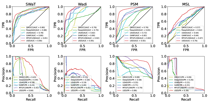
First, we discuss the performance advantages of the USD method by comparing results on five common benchmarks. We list the results for the AUROC and AUPRC metrics in Tables II and III, where the numbers in parentheses represent the variance from five different seed experiments. We report on two variants of USD: one (USD) uses the same hyperparameters across all experiments, and the other (USD*) involves hyperparameter tuning specific to each target dataset. The best results are highlighted in bold. To visualize the benefits of USD performance, the ROC and PR curves on four dataset is showned in Fig. 3. In the ROC and PR curves, the USD method consistently outperforms the baseline methods, demonstrating its robustness and effectiveness in anomaly detection tasks.
Performance improvement. In terms of performance improvements, as shown in Tables II, the USD method shows significant enhancements compared to state-of-the-art methods. These improvements are evident across both PR and AUC curves, particularly on the SWAT dataset with a 5.4% increase in AUROC and a 7.7% increase in AUPRC, and on the MSL dataset with a 6% increase in AUROC and a 7.0% increase in AUPRC. On average, there is a 4.1% increase in AUROC performance and a 7.0% increase in AUPRC performance. The consistent improvements in both AUROC and AUPRC indicate that the USD method has enhanced performance across multiple aspects.
Stability improvement. As shown in Tables II and III and Fig. 3, the stability of the USD method is also noteworthy, exhibiting lower variance across all test datasets compared to traditional methods. This indicates that the USD method is more robust and less sensitive to random initialization, making it a reliable choice for anomaly detection tasks.
Performance potential. Furthermore, by comparing the results of USD and USD*, we find that conducting hyperparameter searches for each dataset can significantly boost model performance. This suggests that our method has good hyperparameter adaptability and considerable potential for further performance enhancements.
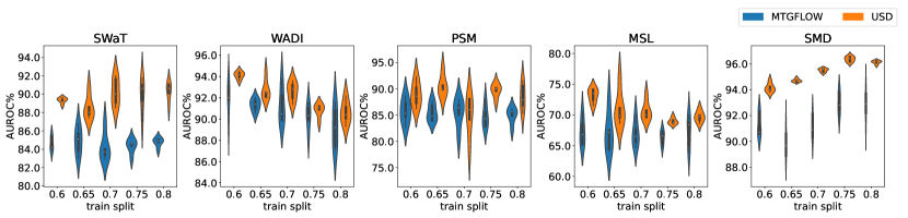
Additional results on difference train/validation splits. To further investigate the influence of anomaly contamination rates, we vary training splits to adjust anomalous contamination rates. For all the above-mentioned datasets, the training split increases from 60% to 80% with 5% stride. We present an average result over five runs in Fig. 4. Although the anomaly contamination ratio of training dataset rises, the anomaly detection performance of MTGFlow remains at a stable high level. This indicates that the proposed USD method is robust to the anomaly contamination ratio of the training dataset.
V-D Visualization of multi-subclass data distributions
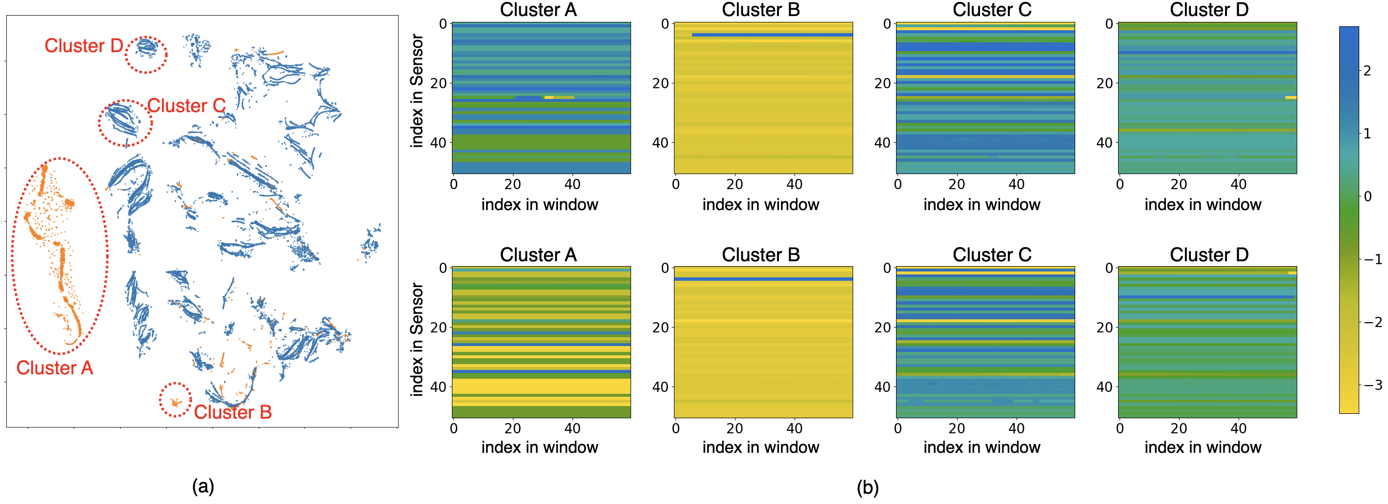
To further investigate the effectiveness of the USD method, we visualize the multi-subclass data distributions on the SWAT dataset. As shown in Fig. 5, the t-SNE visualization of the embedding of USD on SWAT datasets reveals multiple clusters, consistent with the multiple manifold assumption of this paper. The normal and abnormal states are not a single cluster but can be divided into separate subclusters. The heatmaps of individual data points further illustrate the similarity of samples within sub-clusters and the differences between samples in different sub-clusters. This visualization demonstrates the ability of the USD method to capture the diverse patterns present in both normal and abnormal states, enhancing its anomaly detection capabilities.
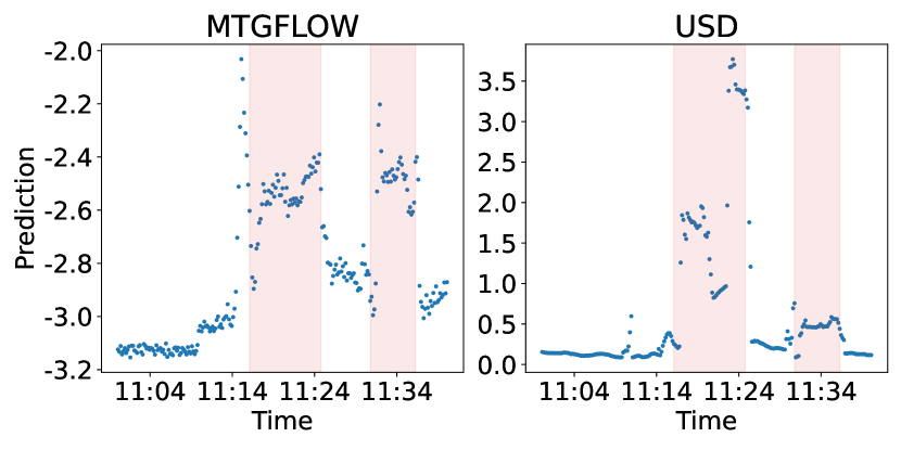
In addition, we present the point plot of the anomalies predict outputs of MTGFLOW and the proposed USD in Fig. 6. The x-axis represents the anomaly index, and the y-axis represents the log-likelihood of the anomaly. Anomalous ground truths are marked by a red background. This indicates that USD is able to detect anomalies more accurately and in a timely manner, outperforming MTGFLOW in terms of anomaly detection performance.
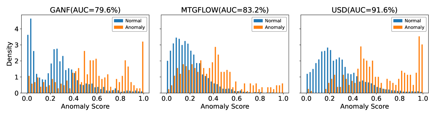
Fig. 7 shows the bar plot of the frequency of normalized anomaly scores on baseline methods and USD. The x-axis represents the anomaly scores, and the y-axis represents the frequency of each score. The normalized anomaly scores of USD are significantly lower than those of GANF and MTGFlow, indicating that USD is more effective at distinguishing between normal and abnormal states.
V-E Ablation Study: The Effect of SCL Loss.
| Method | SWaT | WADI | PSM | MSL | ||
|---|---|---|---|---|---|---|
| USD | 90.2(±0.9) | 94.1(±0.4) | 88.9(±2.4) | 74.2(±2.0) | ||
| w. Gaussian | 88.9(±1.1) | 93.9(±1.7) | 86.7(±2.5) | 72.1(±0.7) | ||
| w/o. SCL | 84.3(±1.5) | 91.7(±1.2) | 85.5(±1.3) | 70.7(±2.4) | ||
| w/o. CL | 84.7(±1.3) | 90.8(±1.4) | 85.9(±1.6) | 69.2(±2.1) | ||
|
84.8(±1.5) | 91.9(±1.1) | 85.7(±1.5) | 67.2(±1.7) |
To assess the effectiveness of each component designed in our model, we conducted a series of ablation experiments. The results of these experiments are presented in Table IV.
We performed controlled experiments to verify the necessity of the Soft Contrastive Learning (SCL) Loss in the UNDA settings across all four datasets. The performance of the proposed USD method is denoted as USD in the table. The variant w/o. SCL represents the model performance with the SCL loss component, , removed from the overall loss function of USD. The variant w. CL indicates the model performance when the SCL loss is replaced by a typical Contrastive Loss (CL), , as defined in Eq. (10).
The results clearly demonstrate that the SCL Loss significantly outperforms the traditional CL loss. We attribute the inferior performance of to its inability to adequately address the view-noise caused by domain bias. Conversely, the SCL loss is more effective at mitigating this issue, leading to better model performance across the datasets.
V-F Hyperparameter Robustness
| Dataset | Window Size | #blocks=1 | #blocks=2 | #blocks=3 | #blocks=4 | #blocks=5 |
|---|---|---|---|---|---|---|
| SWaT | 40 | 92.0(±1.2) | 84.7(±1.2) | 83.3(±2.9) | 81.8(±2.3) | 80.9(±1.7) |
| 60 | 90.2(±0.9) | 86.2(±2.1) | 85.8(±1.8) | 80.3(±2.1) | 82.0(±1.9) | |
| 80 | 89.9(±1.9) | 88.1(±1.4) | 85.6(±3.4) | 83.3(±1.8) | 82.7(±2.0) | |
| 100 | 89.7(±1.7) | 85.1(±1.0) | 84.4(±1.1) | 81.6(±3.6) | 81.2(±2.9) | |
| 120 | 89.8(±1.4) | 86.8(±1.1) | 85.9(±1.9) | 82.7(±3.2) | 83.8(±3.9) | |
| 140 | 90.5(±1.5) | 86.6(±1.5) | 86.7(±1.5) | 85.1(±3.6) | 80.8(±4.1) | |
| 160 | 89.3(±1.7) | 87.7(±1.0) | 86.0(±2.0) | 84.8(±2.7) | 82.7(±2.9) | |
| WADI | 40 | 88.9(±1.0) | 93.6(±0.6) | 93.8(±0.5) | 93.6(±1.1) | 93.1(±0.4) |
| 60 | 90.6(±1.3) | 93.7(±0.6) | 93.8(±0.4) | 93.8(±0.2) | 94.1(±0.4) | |
| 80 | 80.8(±1.1) | 94.1(±0.5) | 93.8(±0.3) | 93.9(±0.5) | 93.9(±0.9) | |
| 100 | 90.0(±0.6) | 93.8(±0.5) | 94.0(±0.4) | 93.8(±0.5) | 94.1(±0.4) | |
| 120 | 90.9(±0.9) | 94.1(±0.9) | 94.1(±0.7) | 93.9(±0.4) | 94.2(±0.4) | |
| 140 | 90.3(±0.8) | 94.4(±0.8) | 94.5(±0.6) | 94.4(±0.8) | 94.3(±0.6) | |
| 160 | 91.8(±2.2) | 94.0(±0.4) | 93.7(±0.4) | 94.9(±1.2) | 94.3(±0.5) | |
| PSM | 40 | 87.9(±2.8) | 87.6(±1.7) | 85.9(±1.9) | 86.4(±2.0) | 86.8(±0.9) |
| 60 | 88.9(±2.4) | 87.4(±1.2) | 87.1(±1.6) | 85.6(±2.0) | 85.9(±2.1) | |
| 80 | 85.2(±5.9) | 86.5(±1.2) | 85.2(±0.7) | 86.3(±1.4) | 85.2(±1.0) | |
| 100 | 85.4(±5.8) | 84.1(±2.0) | 85.4(±1.2) | 86.9(±0.7) | 84.7(±2.3) | |
| 120 | 85.1(±5.4) | 85.2(±1.2) | 85.4(±1.5) | 85.7(±2.4) | 83.6(±1.2) | |
| 140 | 87.3(±2.8) | 86.1(±2.3) | 86.1(±1.2) | 84.8(±1.6) | 86.2(±0.8) | |
| 160 | 86.5(±3.0) | 85.3(±0.8) | 85.6(±4.7) | 84.5(±1.3) | 84.6(±1.2) | |
| MSL | 40 | 71.6(±2.2) | 72.9(±2.5) | 72.9(±2.3) | 72.2(±1.4) | 72.8(±1.2) |
| 60 | 71.4(±2.3) | 74.2(±2.0) | 74.1(±1.5) | 74.0(±0.9) | 73.4(±0.9) | |
| 80 | 71.9(±2.7) | 74.8(±1.4) | 72.9(±1.6) | 74.4(±0.7) | 73.6(±1.4) | |
| 100 | 71.8(±1.3) | 74.3(±1.2) | 72.7(±2.2) | 73.2(±0.5) | 73.4(±1.8) | |
| 120 | 72.3(±2.7) | 75.6(±1.7) | 73.0(±1.3) | 73.2(±1.6) | 73.9(±1.1) | |
| 140 | 70.4(±2.1) | 74.3(±0.7) | 73.3(±1.9) | 73.7(±2.0) | 75.3(±2.2) | |
| 160 | 70.6(±3.4) | 76.0(±1.1) | 75.6(±2.2) | 74.5(±1.6) | 75.0(±1.3) |
Hyperparameter Robustness: Window Size and Number of Blocks. The Table. V presents an ablation study investigating the robustness of hyperparameters, focusing on the window size and number of blocks. Three distinct datasets, SWaT, WADI, and PSM, along with MSL, are evaluated using USD. Our method showcases promising results, with consistently competitive AUROC scores across varying hyperparameter configurations. Notably, the standard deviations accompanying AUROC values indicate a high degree of stability, underscoring the reliability of our approach. Analysis of the table reveals that optimal configurations often coincide with larger window sizes and moderate block numbers, suggesting a preference for capturing broader temporal contexts while maintaining computational efficiency. Additionally, trends indicate that as the number of blocks increases, there’s a discernible improvement in performance, albeit with diminishing returns beyond a certain threshold. This observation highlights the importance of carefully balancing model complexity with computational resources. Overall, the USD method demonstrates robustness and effectiveness in anomaly detection tasks.
Hyperparameter Robustness: Learning rate, , and number of epoch. In order to further investigate the effectiveness of MTGFlow, we give a detailed analysis based on SWaT dataset. We conduct ablation studies on the learning rate, , and the number of epochs. The results are shown in Table. VI, Table. VIII, and Table. VII. The results show that the performance of MTGFlow is relatively stable across different learning rates, , and the number of epochs. This indicates that MTGFlow is robust to hyperparameter changes and can achieve good performance with a wide range of hyperparameters.
| lr | 0.001 | 0.005 | 0.01 | 0.05 | 0.1 | 0.5 |
|---|---|---|---|---|---|---|
| AUROC | 84.5(±4.2) | 90.9(±0.9) | 90.2(±0.9) | 82.3(±1.5) | 82.4(±2.7) | 79.2(±4.1) |
| epoch | 40 | 100 | 200 | 400 | 500 | 1000 |
|---|---|---|---|---|---|---|
| AUROC | 81.4(±2.9) | 85.8(±2.9) | 89.8(±1.4) | 90.2(±0.9) | 90.2(±0.9) | 90.2(±0.9) |
| 0.005 | 0.01 | 0.05 | 0.1 | |
|---|---|---|---|---|
| AUROC | 88.4(±1.8) | 90.2(±0.9) | 90.5(±1.3) | 90.6(±2.6) |
| 0.5 | 1 | 2 | 3 | 4 | 5 | |
|---|---|---|---|---|---|---|
| 1 | 91.2(±1.0) | 90.2(±3.1) | 91.3(±1.7) | 89.8(±1.8) | 90.9(±1.1) | 89.8(±1.8) |
| 2 | 89.0(±2.0) | 90.0(±2.3) | 90.1(±0.7) | 90.6(±1.6) | 90.6(±2.3) | 91.2(±1.9) |
| 3 | 89.8(±2.8) | 90.3(±2.5) | 91.2(±1.7) | 88.6(±2.8) | 91.3(±0.9) | 90.1(±1.8) |
| 4 | 89.9(±1.1) | 89.1(±2.6) | 90.3(±1.0) | 88.7(±2.5) | 90.1(±0.8) | 90.4(±2.7) |
| 5 | 89.2(±3.2) | 90.2(±0.9) | 92.1(±1.1) | 89.0(±2.2) | 90.2(±0.8) | 90.3(±1.1) |
| 6 | 89.3(±0.9) | 90.9(±1.4) | 89.4(±1.2) | 90.0(±1.3) | 89.5(±2.2) | 90.4(±1.9) |
VI Conclusion
In this work, we proposed USD, an unsupervised soft contrastive learning framework for fault detection in multivariate time series data. The proposed method goes beyond the limitations imposed by the Gaussian distribution assumption by using more accurate multi-Gaussian representations. We first designed a neighbor-based unsupervised data augmentation method to generate positive samples for unsupervised soft contrast learning through online data augmentation of multivariate time series data. Then, we computed the loss function for soft contrast learning by incorporating a representation learning head module. Soft contrast learning optimizes the discriminative representation space based on the similarity of local streamforms to better portray the difference between normal and abnormal states. We argued that incorporating soft contrast learning not only enhances the model’s ability to distinguish between normal and abnormal patterns but also captures a wider range of potential anomalies. Experimental evaluations showed that our model performance (AUC and PR) was significantly improved compared to existing fault detection frameworks. Specifically, our approach achieved new enhancements on multiple standard test benchmarks (SWaT, WADI) and operational scenarios with lower false alarm rates and higher detection accuracies. At the same time, we demonstrated, e.g., through visualization, the plausibility of our multi-Gaussian assumptions and the fact that soft-contrast learning can characterize different sub-states well. We summarized the contributions of this paper as follows.
VII Acknowledgements
This work was supported by the Key Research and Development Program of Zhejiang Province (2024C01140). This work was supported by the Key Research and Development Program of Hangzhou (2023SZD0073).
References
- [1] Ahmed Abdulaal, Zhuanghua Liu, and Tomer Lancewicki. Practical approach to asynchronous multivariate time series anomaly detection and localization. In Proceedings of the 27th ACM SIGKDD Conference on Knowledge Discovery & Data Mining, pages 2485–2494, 2021.
- [2] Chuadhry Mujeeb Ahmed, Venkata Reddy Palleti, and Aditya P Mathur. Wadi: a water distribution testbed for research in the design of secure cyber physical systems. In Proceedings of the 3rd international workshop on cyber-physical systems for smart water networks, pages 25–28, 2017.
- [3] Lynton Ardizzone, Carsten Lüth, Jakob Kruse, Carsten Rother, and Ullrich Köthe. Guided image generation with conditional invertible neural networks. arXiv preprint arXiv:1907.02392, 2019.
- [4] Julien Audibert, Pietro Michiardi, Frédéric Guyard, Sébastien Marti, and Maria A Zuluaga. Usad: unsupervised anomaly detection on multivariate time series. In Proceedings of the 26th ACM SIGKDD International Conference on Knowledge Discovery & Data Mining, pages 3395–3404, 2020.
- [5] Raghavendra Chalapathy and Sanjay Chawla. Deep learning for anomaly detection: A survey. arXiv preprint arXiv:1901.03407, 2019.
- [6] Ting Chen, Simon Kornblith, Mohammad Norouzi, and Geoffrey Hinton. A simple framework for contrastive learning of visual representations. pages 1597–1607, 2020.
- [7] Xuanhao Chen, Liwei Deng, Feiteng Huang, Chengwei Zhang, Zongquan Zhang, Yan Zhao, and Kai Zheng. Daemon: Unsupervised anomaly detection and interpretation for multivariate time series. In 2021 IEEE 37th International Conference on Data Engineering (ICDE), pages 2225–2230. IEEE, 2021.
- [8] Enyan Dai and Jie Chen. Graph-augmented normalizing flows for anomaly detection of multiple time series. In International Conference on Learning Representations, 2021.
- [9] Jonathan Goh, Sridhar Adepu, Khurum Nazir Junejo, and Aditya Mathur. A dataset to support research in the design of secure water treatment systems. In International conference on critical information infrastructures security, pages 88–99. Springer, 2016.
- [10] Sachin Goyal, Aditi Raghunathan, Moksh Jain, Harsha Vardhan Simhadri, and Prateek Jain. Drocc: Deep robust one-class classification. In International Conference on Machine Learning, pages 3711–3721. PMLR, 2020.
- [11] Jean-Bastien Grill, Florian Strub, Florent Altché, Corentin Tallec, Pierre H Richemond, Elena Buchatskaya, Carl Doersch, Bernardo Avila Pires, Zhaohan Guo, Mohammad Gheshlaghi Azar, et al. Bootstrap your own latent: A new approach to self-supervised learning. In Advances in Neural Information Processing Systems, volume 33, pages 21271–21284, 2020.
- [12] Kaiming He, Haoqi Fan, Yuxin Wu, Saining Xie, and Ross Girshick. Momentum contrast for unsupervised visual representation learning. In Proceedings of the IEEE/CVF Conference on Computer Vision and Pattern Recognition, pages 9729–9738, 2020.
- [13] Kyle Hundman, Valentino Constantinou, Christopher Laporte, Ian Colwell, and Tom Soderstrom. Detecting spacecraft anomalies using lstms and nonparametric dynamic thresholding. In Proceedings of the 24th ACM SIGKDD international conference on knowledge discovery & data mining, pages 387–395, 2018.
- [14] Ning Huyan, Dou Quan, Xiangrong Zhang, Xuefeng Liang, Jocelyn Chanussot, and Licheng Jiao. Unsupervised outlier detection using memory and contrastive learning. arXiv preprint arXiv:2107.12642, 2021.
- [15] Rui Li, Wim JC Verhagen, and Richard Curran. A systematic methodology for prognostic and health management system architecture definition. Reliability Engineering & System Safety, 193:106598, 2020.
- [16] Siyuan Li, Zicheng Liu, Zelin Zang, Di Wu, Zhiyuan Chen, and Stan Z Li. Genurl: A general framework for unsupervised representation learning. IEEE Transactions on Neural Networks and Learning Systems, 2024.
- [17] Stan Z Li, Zelin Zang, and Lirong Wu. Deep manifold transformation for nonlinear dimensionality reduction. arXiv preprint arXiv:2010.14831, 2020.
- [18] Stan Z Li, Zelin Zang, and Lirong Wu. Markov-lipschitz deep learning. arXiv preprint arXiv:2006.08256, 2020.
- [19] Chen Liu, Shibo He, Qihang Zhou, Shizhong Li, and Wenchao Meng. Large language model guided knowledge distillation for time series anomaly detection. arXiv preprint arXiv:2401.15123, 2024.
- [20] Pankaj Malhotra, Anusha Ramakrishnan, Gaurangi Anand, Lovekesh Vig, Puneet Agarwal, and Gautam Shroff. Lstm-based encoder-decoder for multi-sensor anomaly detection. arXiv preprint arXiv:1607.00148, 2016.
- [21] Nam D Nguyen, Jiawei Huang, and Daifeng Wang. A deep manifold-regularized learning model for improving phenotype prediction from multi-modal data. Nature computational science, 2(1):38–46, 2022.
- [22] Lukas Ruff, Robert Vandermeulen, Nico Goernitz, Lucas Deecke, Shoaib Ahmed Siddiqui, Alexander Binder, Emmanuel Müller, and Marius Kloft. Deep one-class classification. In International conference on machine learning, pages 4393–4402. PMLR, 2018.
- [23] Lukas Ruff, Robert A Vandermeulen, Nico Görnitz, Alexander Binder, Emmanuel Müller, Klaus-Robert Müller, and Marius Kloft. Deep semi-supervised anomaly detection. arXiv preprint arXiv:1906.02694, 2019.
- [24] Ya Su, Youjian Zhao, Chenhao Niu, Rong Liu, Wei Sun, and Dan Pei. Robust anomaly detection for multivariate time series through stochastic recurrent neural network. In Proceedings of the 25th ACM SIGKDD international conference on knowledge discovery & data mining, pages 2828–2837, 2019.
- [25] Jing Wang, Shikuan Shao, Yunfei Bai, Jiaoxue Deng, and Youfang Lin. Multiscale wavelet graph autoencoder for multivariate time-series anomaly detection. IEEE Transactions on Instrumentation and Measurement, 72:1–11, 2022.
- [26] Siqi Wang, Yijie Zeng, Xinwang Liu, En Zhu, Jianping Yin, Chuanfu Xu, and Marius Kloft. Effective end-to-end unsupervised outlier detection via inlier priority of discriminative network. Advances in neural information processing systems, 32, 2019.
- [27] Xiaolei Yu, Zhibin Zhao, Xingwu Zhang, Xuefeng Chen, and Jianbing Cai. Statistical identification guided open-set domain adaptation in fault diagnosis. Reliability Engineering & System Safety, 232:109047, 2023.
- [28] Zelin Zang, Shenghui Cheng, Hanchen Xia, Liangyu Li, Yaoting Sun, Yongjie Xu, Lei Shang, Baigui Sun, and Stan Z. Li. Dmt-ev: An explainable deep network for dimension reduction. IEEE Transactions on Visualization and Computer Graphics, 30(3):1710–1727, 2024.
- [29] Zelin Zang, Siyuan Li, Di Wu, Ge Wang, Kai Wang, Lei Shang, Baigui Sun, Hao Li, and Stan Z Li. Dlme: Deep local-flatness manifold embedding. In European Conference on Computer Vision, pages 576–592. Springer, 2022.
- [30] Zelin Zang, Hao Luo, Kai Wang, Panpan Zhang, Fan Wang, Stan. Z Li, and Yang You. Boosting unsupervised contrastive learning using diffusion-based data augmentation from scratch, 2023.
- [31] Zelin Zang, Lei Shang, Senqiao Yang, Fei Wang, Baigui Sun, Xuansong Xie, and Stan Z Li. Boosting novel category discovery over domains with soft contrastive learning and all in one classifier. In Proceedings of the IEEE/CVF International Conference on Computer Vision, pages 11858–11867, 2023.
- [32] Liangwei Zhang, Jing Lin, Haidong Shao, Zhicong Zhang, Xiaohui Yan, and Jianyu Long. End-to-end unsupervised fault detection using a flow-based model. Reliability Engineering & System Safety, 215:107805, 2021.
- [33] Bo Zhao, Xianmin Zhang, Qiqiang Wu, Zhuobo Yang, and Zhenhui Zhan. A novel unsupervised directed hierarchical graph network with clustering representation for intelligent fault diagnosis of machines. Mechanical Systems and Signal Processing, 183:109615, 2023.
- [34] Qihang Zhou, Jiming Chen, Haoyu Liu, Shibo He, and Wenchao Meng. Detecting multivariate time series anomalies with zero known label. In Proceedings of the AAAI Conference on Artificial Intelligence, volume 37, pages 4963–4971, 2023.
- [35] Qihang Zhou, Shibo He, Haoyu Liu, Jiming Chen, and Wenchao Meng. Label-free multivariate time series anomaly detection. IEEE Transactions on Knowledge and Data Engineering, 2024.
- [36] Bo Zong, Qi Song, Martin Renqiang Min, Wei Cheng, Cristian Lumezanu, Daeki Cho, and Haifeng Chen. Deep autoencoding gaussian mixture model for unsupervised anomaly detection. In International conference on learning representations, 2018.
- [37] Tiago Zonta, Cristiano André Da Costa, Rodrigo da Rosa Righi, Miromar Jose de Lima, Eduardo Silveira da Trindade, and Guann Pyng Li. Predictive maintenance in the industry 4.0: A systematic literature review. Computers & Industrial Engineering, 150:106889, 2020.
A. Details of SCL loss
A.1 Details of the transformation from Eq. (10) to Eq. (11)
We start with (Eq. (10)), then
We are only concerned with the second term that has the gradient. Let are positive pair and are negative pairs. The overall loss associated with point is:
We focus on the case where the similarity is normalized, . The data and data is the negative samples, then is near to , is near to , thus the is near to 1, and near to 0. We have
We denote and by a uniform index and use to denote the homology relation of .
we define the similarity of data and data as and the dissimilarity of data and data as .
A.2 The proposed SCL loss is a smoother CL loss
This proof tries to indicate that the proposed SCL loss is a smoother CL loss. We discuss the differences by comparing the two losses to prove this point. the forward propagation of the network is, , . We found that we mix and in the main text, and we will correct this in the new version. So, in this section , is also correct.
Let satisfy -Lipschitz continuity, then where is a Lipschitz constant. The difference between loss and loss is,
| (16) |
Because the , the proposed SCL loss is the soft version of the CL loss. if , we have:
| (17) |
then:
| (18) |
Based on Eq.(18), we find that if is neighbor () and , there is no difference between the CL loss and SCL loss . When if , the difference between the loss functions will be the function of . The CL loss only minimizes the distance between adjacent nodes and does not maintain any structural information. The proposed SCL loss considers the knowledge both comes from the output of the current bottleneck and data augmentation, thus less affected by view noise.
Details of Eq. (16). Due to the very similar gradient direction, we assume . The contrastive learning loss is written as,
| (19) |
where indicates whether and are augmented from the same original data.
The SCL loss is written as:
| (20) |
According to Eq. (4) and Eq. (5), we have
| (21) | ||||
For ease of writing, we use distance as the independent variable, , .
The difference between the two loss functions is:
| (22) | ||||
Substituting the relationship between and , , we have
| (23) |
We assume that network to be a Lipschitz continuity function, then
| (24) |
We construct the inverse mapping of to ,
| (25) |
and then there exists :
| (26) |
| (27) |
A.3 SCL is better than CL in view-noise
To demonstrate that compared to contrastive learning, the proposed SCL Loss has better results, we first define the signal-to-noise ratio (SNR) as an evaluation metric.
| (28) |
where means the expectation of positive pair loss, means the expectation of noisy pair loss.
This metric indicates the noise-robust of the model, and obviously, the bigger this metric is, the better.
In order to prove the soft contrastive learning’s SNR is larger than contrastive learning’s, we should prove:
| (29) |
Obviously, when it is the positive pair case, is large if and small if .
Anyway, when it is the noisy pair case, is small if and large if .
First, we organize the and into 2 cases, and , for writing convenience, we write as and , respectively.
| (30) |
| (31) |
M is the ratio of the number of occurrences of to . So, we could get:
| (32) | ||||
In the case of positive pair, converges to 1 and converges to 0.
Because we have bounded that , so we could easily get:
| (33) |
Also, we could get:
| (34) |
So we get:
| (35) |
And for the case of noise pair, the values of and are of opposite magnitude, so obviously, there is .
So the formula Eq. (29) has been proved.
B. Model Hyperparameter Settings and Model Hyperparameter Settings
The model used in this article involves the setting of multiple hyperparameters that are critical to model performance and reproducibility of results. In order to enable readers to accurately understand and reproduce our experimental results, we list the hyperparameter settings of the corresponding experiments.
This appendix includes the following three tables, corresponding to the hyperparameter settings of the model under different experimental conditions in the paper:
- 1.
- 2.
- 3.
| SWaT | Wadi | PSM | MSL | SMD | ||
|---|---|---|---|---|---|---|
| alpha | 0.1 | 0.1 | 0.1 | 0.1 | 0.1 | |
| batch size | 128 | 64 | 128 | 128 | 256 | |
| k | 10 | 20 | 20 | 20 | 30 | |
| loss weight manifold ne | 5 | 5 | 5 | 5 | 5 | |
| loss weight manifold po | 1 | 1 | 1 | 1 | 5 | |
| lr | 0.01 | 0.002 | 0.002 | 0.002 | 0.1 | |
| n blocks | 1 | 5(4) | 1 | 2 | 1 | |
| name | SWaT | Wadi | PSM | MSL | 28 sub-datasets | |
| seed | 15,16,17,18,19 | 15,16,17,18,19 | 15,16,17,18,19 | 15,16,17,18,19 | 15,16,17,18,19 | |
| window size | 60(40) | 60 (160) | 60 | 60(160) | 60 | |
| train split | 0.6* | 0.6 | 0.6 | 0.6 | 0.6 | |
| SWaT | Wadi | PSM | MSL | SMD | ||
| alpha | 0.1 | 0.1 | 0.1 | 0.1 | 0.1 | |
| batch size | 128 | 64 | 128 | 128 | 256 | |
| k | 10 | 20 | 20 | 20 | 30 | |
| loss weight manifold ne | 5 | 5 | 5 | 5 | 5 | |
| loss weight manifold po | 1 | 1 | 1 | 1 | 5 | |
| lr | 0.01 | 0.002 | 0.002 | 0.002 | 0.1 | |
| n blocks | 1 | 5 | 1 | 2 | 1 | |
| name | SWaT | Wadi | PSM | MSL | 28 sub-datasets | |
| seed | 15,16,17,18,19 | 15,16,17,18,19 | 15,16,17,18,19 | 15,16,17,18,19 | 15,16,17,18,19 | |
| train split | 0.6, 0.65, 0.7, 0.75, 0.8 | |||||
| window size | 60 | 60 | 60 | 60 | 60 | |
| SWaT | Wadi | PSM | MSL | ||
|---|---|---|---|---|---|
| alpha | 0.1 | 0.1 | 0.1 | 0.1 | |
| batch size | 128 | 64 | 128 | 128 | |
| k | 10 | 20 | 20 | 20 | |
| loss weight manifold ne | 5 | 5 | 5 | 5 | |
| loss weight manifold po | 1 | 1 | 1 | 1 | |
| lr | 0.01 | 0.002 | 0.002 | 0.002 | |
| name | SWaT | Wadi | PSM | MSL | |
| seed | 15,16,17,18,19 | 15,16,17,18,19 | 15,16,17,18,19 | 15,16,17,18,19 | |
| train plit | 0.6* | 0.6 | 0.6 | 0.6 | |