GeoAdaLer: Geometric Insights into Adaptive Stochastic Gradient Descent Algorithms

Abstract

The Adam optimization method has achieved remarkable success in addressing contemporary challenges in stochastic optimization. This method falls within the realm of adaptive sub-gradient techniques, yet the underlying geometric principles guiding its performance have remained shrouded in mystery, and have long confounded researchers. In this paper, we introduce GeoAdaLer (Geometric Adaptive Learner), a novel adaptive learning method for stochastic gradient descent optimization, which draws from the geometric properties of the optimization landscape. Beyond emerging as a formidable contender, the proposed method extends the concept of adaptive learning by introducing a geometrically inclined approach that enhances the interpretability and effectiveness in complex optimization scenarios.

1 Introduction

Stochastic gradient descent (SGD) optimization methods play an important role in various scientific fields. When applied to machine learning algorithms, the objective is to adjust a set of parameters with the goal of optimizing an objective function. This optimization usually involves a series of iterative adjustments made to the parameters in each step as the algorithm progresses [5]. In the vanilla gradient descent approach, the magnitude of the gradient is the predominant annealing factor causing the algorithm to take larger steps when you are away from the optimum and smaller steps when closer to an optimum [13]. This method, however, becomes less effective near an optimal point, necessitating the selection of a smaller learning rate, which in turn affects the speed of convergence. The raw magnitude of the gradient does not always align with the optimal descent step size, thus necessitating a manually chosen learning rate. If the learning rate is too big, overshooting may occur and convergence rate is slow if the learning rate is too small. This challenge has led to the development of adaptive learning algorithms [11]. In this paper, we explore gradient descent algorithms that optimize the objective function with emphasis on the update rule. In this context, we focus on the update rule by breaking it into three components: the learning rate, the annealing factor, and the descent direction. This approach allows us to evaluate the effectiveness of an algorithm by examining the impact of its learning rate, annealing factor, and descent direction on the optimization process.

In this paper, we propose GeoAdaLer (short for Geometric Adaptive Learner) – a new adaptive learning method for SGD optimization that is based on the geometric properties of the objective landscape. In this method, we use cosine of $\theta$ (where $\theta$ is the acute angle between the normal to the tangent hyperplane and the horizontal hyperplane) as an annealing factor, which takes values close to zero when the optimization is traversing points close to an optimum and close to one for points far away from an optimum. Our method has surprising similarities to other adaptive learning methods.

Some of the advantages of GeoAdaLer is that it introduces a geometric approach for the annealing factor and outperforms standard SGD optimization methods due to the cosine of $\theta$. Through both theoretical analysis and empirical observation, we identified similarities between our proposed method and other adaptive learning techniques. Our method not only enhances the understanding of existing algorithms but also opens up possibilities for more interpretable deep learning approaches.

Additionally, we analyze the convergence of GeoAdaLer. We frame the optimization process as a fixed-point problem and split the analysis into deterministic and stochastic cases. Under the deterministic framework, we assume convexity and the existence of a finite optimal value. We utilize the Lipschitz continuity property of the gradient to establish upper bounds of convergence. We further employ the co-coercivity and quadratic upper bound properties to establish the lower bounds of convergence [16]. Under the stochastic framework, we employ the regret function, which measures the overall difference between our method and the known optimum point, ensuring that as time tends to infinity, the regret function over time tends to zero. By ensuring that the upper bound of the regret function goes to zero, we determine the overall convergence of the stochastic method to an optimum point. Both the deterministic and stochastic analyses demonstrate the robustness of GeoAdaLer and enhance our understanding of its practical applications.

2 Related Work

In the field of adaptive stochastic gradient descent algorithms, we continue to see improvements, often due to the need to address shortcomings of previous methods. The pioneering approach is AdaGrad, which focuses on the concept of per-parameter adaptive learning rates. The foundation of AdaGrad is also the source of its limitation: the monotonic accumulation of squared gradients that could prematurely stifle learning rates [17].

Subsequent optimizers like AdaDelta, RMSprop, and the popular Adam sought to address this issue [5, 15, 17]. AdaDelta introduced a decaying average of past squared gradients, while RMSprop utilized a similar exponential decay mechanism to limit the aggressive reduction in learning rates. Adam combined RMSprop’s adaptive learning rates with the concept of momentum for smoother updates. However, Adam has been challenged by AMSGrad which modifies the algorithm in order to imbue it with "long term memory" which addresses issues with sub-optimal convergence under specific conditions and improves empirical performance [12]. As pointed out by [10, 14, 18], the assumptions on the hyperparameters of Adam were made before constructing the counter examples in [12]. Insights gained from these examples are invaluable for the ongoing exploration of stochastic gradient descent algorithms.

The literature on adaptive optimization algorithms for SGD reveals that each algorithm addresses the problems evident in its predecessors. The iterative approach, while successful in many ways, arguably emphasizes the lack of fundamental intuition regarding the dynamics of the AdaGrad family of optimizers.

GeoAdaLer is a novel adaptive learning method for SGD, employing the properties of the objective landscape. The innovative idea behind the GeoAdaLer approach is that the acute angle between the normal to the tangent plane at $x$ and the horizontal plane conveys significant curvature-related information. This information could potentially recover the power of second order methods, which are not feasible in large-scale machine learning optimization. An understanding of this geometric approach to analyze adaptive methods for SGD can shed new light on the behavior of other algorithms in the AdaGrad family, potentially revealing the rationale for their strengths and weaknesses.

By discussing the geometric implications of adaptive step processes, we are able to potentially come up with optimizers that:

• have more optimal annealing: A geometric perspective could inform strategies to control learning rate decay more effectively, preventing premature convergence or extensively slow convergence.

• provide parameter-sensitive adaptivity: The geometry may reveal how to tailor updates for individual parameters in a more principled manner.

• increase robustness: Understanding the geometric implications could lead to optimizers that are less dependent on sensitive hyper-parameter tuning.

In essence, a geometric framework promises to move beyond the reactive development pattern, allowing us to proactively design adaptive optimizers that address the core issues in the AdaGrad family with greater intuition and foresight.

3 Mathematical Formulation

3.1 Deterministic Optimization

Consider the minimization of the objective functional $f:\mathbb{R}^{n}\to\mathbb{R}$ using the gradient descent algorithm. The vanilla gradient descent (GD) algorithm that maximizes the benefit of gradient annealing for smooth functions is

$$x_{t+1}=x_{t}+\delta x_{t}$$ (1)

where $\delta x_{t}=-\gamma g_{t}$ and $g_{t}$ is the gradient of the objective function at time $t$. This is the update step and is largely responsible for how far a step is taken in the descent direction. To see its real contribution, we decompose it further into

$$\delta x_{t}=-\gamma|g_{t}|\overline{g_{t}}$$ (2)

where $\gamma$ is the learning rate which is responsible for manually scaling the step size,$|g_{t}|$ which is our annealing factor and lastly $-\overline{g_{t}}$ which gives us our optimal descent direction.

We find that the annealing factor tends to be sub-optimal and can cause overshooting which we need to compensate for by applying a smaller learning rate, increasing convergence time [11].

To combat this this issue we propose an annealing factor based on the cosine of $\theta$, where $\theta$ is the acute angle between the normal to the tangent hyperplane and the horizontal hyperplane.

Theorem 1 (Geohess).

Let $\theta$ be the acute angle between the normal to an objective function $f:\mathbb{R}^{n}\to\mathbb{R}$ which is differentiable at $x$. Let $\|\cdot\|$ be the norm induced by the inner product on $\mathbb{R}^{n}$. Then

$$\cos\theta=\frac{\|\nabla f(x)\|}{\sqrt{\|\nabla f(x)\|^{2}+1}}$$ (3)

Proof.

Let $x_{i}$ be an arbitrary point in $\mathbb{R}^{n}$. Then $[-f(x_{i}),1]^{T}$ is orthogonal to $[x-x_{i},y-f(x_{i})]$ where $x$ and $y$ lie on the tangent hyperplane to $f$ at $x_{i}$. i.e., $[-f(x_{i}),1]^{T}$ is normal to $[x-x_{i},y-f(x_{i})]$. Let $\theta$ be the angle this normal makes with the horizontal hyperplane at the point $(x_{i},f(x_{i}))$ in the descent direction $-\nabla f(x_{i})$, i.e., a vector parallel to $[-\nabla f(x_{i}),0]$. Then by vector calculus,

$$\cos\theta =\frac{[-f(x_{i}),1]^{T}\cdot[-f(x_{i}),0]^{T}}{\|[-f(x_{i}),1]^{T}\|\|[-f(x_{i}),0]^{T}\|}=\frac{\|\nabla f(x_{i})\|}{\sqrt{\|\nabla f(x_{i})\|^{2}+1}}$$ (4)

as required. ∎

The proposed GeoAdaLer update step is as follows:

$$\delta x_{t}=-\gamma\,\overline{g_{t}}\cos\theta=-\gamma\frac{\|g_{t}\|}{\sqrt{\|g_{t}\|^{2}+1}}\overline{g_{t}}$$ (5)

Equation (5) follows from the Geohess theorem (Theorem 1). In equation (5), if $g_{t}$ is zero, then the update step is zero and algorithm has converged. If $g_{t}$ is not zero, then equation (5) reduces to

$$\delta x_{t}=-\gamma\frac{1}{\sqrt{\|g_{t}\|^{2}+1}}g_{t}$$

3.2 Properties of GeoAdaLer Annealing Factor

The acute angle $\theta$ depends on $g_{t}$, and therefore, the annealing factor possesses the following properties:

1. $\displaystyle\frac{\|g_{t}\|}{\sqrt{\|g_{t}\|^{2}+1}}\to 1\qquad\text{as}\quad g_{t}\to\infty$

2. $\displaystyle\frac{\|g_{t}\|}{\sqrt{\|g_{t}\|^{2}+1}}\to 0\qquad\text{as}\quad g_{t}\to 0$

In practice, we do not want $g_{t}\to\infty$ but as long as the magnitude of the gradient is large, the sufficiency in item 1 is guaranteed. Of utmost importance is item 2.

In comparison to gradient annealing in SGD, we find that $\cos\theta$ possesses an logarithmic decay as a function of $g_{t}$ as it tends to an optimum, resulting in a much more controllable annealing while standard SGD decays linearly.

The algorithm for GeoAdaLer is given in Algorithm 2.Note: The deterministic setting is achieved by using the objective function over the entire dataset instead of the stochastic objective function, in which case we set $\beta=0$.

3.3 Stochastic Optimization

Online learning and stochastic optimization are closely linked and can be essentially used interchangeably [3, 2]. In online learning, the learner iteratively predicts a point $x_{t}\in X\subseteq\mathbb{R}^{d}$, often representing a weight vector that assigns importance values to different features. The objective of the learner is to minimize regret compared to a fixed predictor $x^{*}$ within the closed convex set $x_{t}\in X\subseteq\mathbb{R}^{d}$ across a sequence of functions $\{f_{1},f_{2},\cdots\}$.

Geometrically, gradients are vectors and have directions. Under a suitable distribution, a convex hull of these gradients approximates the true gradient for stochastic optimizations. In experiments such as deep neural networks where the training data is fixed over each epoch and each input to the network determines an instance of the stochastic objective, the arithmetic average with discrete uniform distribution suffices, and in this case, there is a one-to-one correspondence between the training data and the stochastic objective functions. Thus, at the current iteration $t$ corresponding to an epoch $e$, the expected gradient is

$$m_{t}=\frac{1}{n}\sum_{i=1}^{n}g_{i},\quad\text{for}\quad t\mod n=0,$$ (6)

where $n$ is the number of samples. The average gradient $m_{t}$ is assumed to be the gradient of the expected objective function. GeoAdaLer as in the deterministic case can then be applied with the aim of proceeding in the direction that produces the maximum decrease along the expected objective. Algorithm 1 summarizes the update at iterations $t$ corresponding to an epoch, when all the training data has been seen [19]. We call this update type GeoAdaU, signifying the use of uniform distribution to approximate expectation.

Algorithm 1 GeoAdaU

$\gamma$ : Learning rate

$f_{t}(x)$ : Stochastic objective function

$x_{0}$ : Initial parameter vector

$t\leftarrow 1$

$m_{0}\leftarrow 0$

while $x_{t}$ not converged do

     $g_{t}\leftarrow\nabla_{x}f_{t}(x_{t})$ (Get gradients w.r.t stochastic objective)

     $m_{t}=m_{t-1}+g_{t}$

     if $t\mod n=0$ then

         $m_{t}=m_{t}/n$

         $x_{t+1}=x_{t}-\gamma\cdot m_{t}/\sqrt{\|m_{t}\|^{2}+1}$ (Update parameters)

         $m_{t}\leftarrow 0$

     end if

     $t\leftarrow t+1$

end while

return $x_{t}$

Algorithm 1 is simple to implement and does not require extra storage or computational power. However, we observe empirically that the convergence is slow, and this could be attributed to the waiting time to compute all gradients over the entire datasets before an update occurs. Furthermore, in online learning scenarios where data arrives in streams, GeoAdaU is not a suitable option. This is due to challenges involved in determining an appropriate number of observations, as well as the presence of potential temporal variations in the data. A common and intuitive approach to approximating the expected gradient is by employing an exponential moving average (EMA). We introduce a momentum-like term to replace the instantaneous gradient, thereby mitigating stochastic fluctuations and revealing underlying trends in the gradient values. That is,

$$m_{t+1}=\beta m_{t}+(1-\beta)g_{t}.$$ (7)

where $\beta\in[0,1)$. The term $\beta$ is constructed as a weighted average of the historical gradients and the current gradient. This modification enhances our ability to approximate the true underlying gradient more effectively in time. It also has the ability to update and learn as new streams of data are observed.

Algorithm 2 presents a pseudo-code of the proposed GeoAdaLer learning method.

Algorithm 2 GeoAdaLer

$\gamma$ : Learning rate

$\beta$ : Exponential decay rate for weighted average

$f_{t}$ : Stochastic objective function

$x_{0}$ : Initial parameter vector

$t\leftarrow 0$

while $x_{t}$ not converged do

     $g_{t}\leftarrow\nabla f_{t}(x_{t})$ (Get gradients w.r.t stochastic objective)

     if $t=0$ then

         $m_{t}\leftarrow g_{t}$ (initial weighted average)

     else

         $m_{t}=\beta m_{t-1}+(1-\beta)g_{t}$ (Updated weighted average)

     end if

     $x_{t+1}=x_{t}-\gamma\cdot m_{t}/(\sqrt{\|m_{t}\|^{2}+1})$ (Update parameters)

     $t\leftarrow t+1$

end while

return $x_{t}$

Learning scenarios in which the total number of training samples is unknown a priori can be treated as online learning problems, which is ubiquitous in machine learning tasks. Therefore, we do not delve further into GeoAdaU but instead use it to illustrate the importance of a well-designed stochastic gradient descent method, which significantly relies on the performance of its (deterministic) gradient descent counterpart. This emphasizes the significance of the GeoAdaLer algorithm, marking a pioneering attempt to unify these concepts, which seem to be diverging in the literature.

3.3.1 GeoAdaMax

Due to stochasticity and varying frequencies of occurrence of certain model inputs, such as in deep neural networks, adaptive stochastic gradient descent methods sometimes encounter issues with non-increasing squared gradients. For instance, consider the convex objective function presented in [12], defined as follows:

$$f_{t}(x)=\begin{cases}Cx,&\text{if }t\mod 3=1\\ -x,&\text{otherwise},\end{cases}$$

In such scenarios, the adaptive step employed by the optimizer can still function effectively as a form of annealing, but the natural adaptive step leads to a suboptimality. In such scenerios, applying the standard adaptive steps of Adam, standard GeoAdaLer may lead to a sub optimalities.

To address this problem, an approach was developed by Reddi et. al.[12], which involves retaining the maximum of the normalizing denominator over iterations. This approach reduces to a self scaling SGD with momentum. By implementing similar idea, we observe related results for GeoAdaLer. Geometrically, this implies that our method fixes the magnitude of the normal vector over all subsequent iterations, resulting in a shallower acute angle compared to the standard GeoAdaLer [12].

Algorithm 3 GeoAdaMax

$\gamma$ : Learning rate

$\beta$ : Exponential decay rate for weighted average

$f_{t}$ : Stochastic objective function

$x_{0}$ : Initial parameter vector

$t\leftarrow 0$

$u_{t}\leftarrow 0$

while $x_{t}$ not converged do

     $g_{t}\leftarrow\nabla f_{t}(x_{t})$ (Get gradients w.r.t stochastic objective)

     if $t=0$ then

         $m_{t}\leftarrow g_{t}$ (initial weighted average)

     else

         $m_{t}=\beta m_{t-1}+(1-\beta)g_{t}$ (Updated weighted average)

     end if

     $u_{t}=max(\|m_{t}\|^{2}+1,u_{t-1})$

     $x_{t+1}=x_{t}-\gamma\cdot m_{t}/(\sqrt{u_{t}})$ (Update parameters)

     $t\leftarrow t+1$

end while

return $x_{t}$

4 Relationship to the AdaGrad Family

The AdaGrad family of adaptive SGD methods adjusts learning rates based on the accumulation of past gradients, typically squaring and summing these gradients to moderate the learning rate. AdaGrad itself directly accumulates these squared gradients, while variants like RMSprop and Adam introduce a decay factor to mitigate the rapid decrease in learning rate, promoting a smoother and more sustained convergence [3, 4, 5].

Mathematically, we have $G_{t}=\psi(G_{t-1},g_{t})$ where $\psi$ is some quadratic mapping. For AdaGrad, $\psi(G_{t-1},g_{t})=G_{t-1}\oplus g_{t}$. For RMSprop and Adam, it is the case that $\psi(G_{t-1},g_{t})=\beta G_{t-1}\oplus(1-\beta)g_{t}^{2}$. Despite stemming from different motivations, Geodaler update bears some striking resemblance to this update rule. For this, $\psi(G_{t-1},g_{t})=\beta G_{t-1}+(1-\beta)g_{t}$ and so $G_{t}=\sqrt{\|\psi(G_{t-1},g_{t})\|^{2}+1}$. Note that the AdaGrad family uses a component-wise sum and product, whereas GeoAdaLer uses the usual sum and product but takes the norm of the squared EMA gradients average.

A notable distinction between GeoAdaLer and the AdaGrad family is the role of epsilon. In the AdaGrad family, epsilon is set to a low value, primarily contributing to the numerical stability of the solution. However, in GeoAdaLer, epsilon serves a different purpose. By replacing one in the denominator of our original formulation (i.e., $G_{t}=\sqrt{\|\psi(G_{t-1},g_{t})\|^{2}+\epsilon},\epsilon>0$), we find that GeoAdaLer’s epsilon now controls the normal vector orientation with respect to the tangent hyperplane. When epsilon is equal to one, the normal vector is orthogonal to the tangent hyperplane. For epsilon values less than one, the angle between the normal vector and the tangent hyperplane becomes acute, aligned with the negative gradient direction. Conversely, when epsilon exceeds one, the angle becomes obtuse with respect to the steepest descent direction. Adjusting epsilon can thus facilitate faster convergence of the GeoAdaLer algorithm. For specific applications, reducing the value of epsilon may be beneficial. This approach is akin to what is obtainable in the GeoAdaMax setting, where the normal vector contributing to the adaptive learning is fixed at its maximum.

5 Convergence Analysis

5.1 Deterministic Setting

We analyze the convergence of GeoAdaLer, first for the deterministic case, and then for the stochastic setting. Our setup remains the same, namely:

$$\underset{x}{\text{minimize}}\,f(x)$$ (8)

using the new adaptive gradient descent (GeoAdaLer) method where $f:\mathbb{R}^{n}\to\mathbb{R}$ is an objective function. We recast the optimization problem (8) into a fixed point problem. Let $T:\mathbb{R}^{n}\to\mathbb{R}^{n}$ be a nonlinear operator defined as:

$$Tx =\left(I-\gamma\frac{\nabla f}{\sqrt{\|\nabla f\|^{2}+1}}\right)(x)$$ (9)

where $I$ is the identity map.

Theorem 2.

Let $f:\mathbb{R}^{d}\to\mathbb{R}$ be continuous and $\nabla f$ Lipschitz continuous with $\gamma\leq\frac{1}{L}$ where $L$ is the Lipschitz constant for $\nabla f$. Assume $f$ attains an optimal value at $x^{*}=\arg\min_{x}f(x)$. Then $T$ defined in (9) is a contraction map with contraction parameter $\alpha=\sqrt{1+\gamma^{2}L_{G}^{2}-2\gamma\frac{L_{G}^{2}}{L}}$ where $L_{G}$ is the Lipschitz constant for $\displaystyle\frac{\nabla f}{\sqrt{\|\nabla f\|^{2}+1}}$ and $\|\cdot\|$ is the Euclidean norm in $\mathbb{R}^{n}$. That is

$$\|Tx-Ty\|\leq\alpha\|x-y\|.$$ (10)

A critical component of Theorem 2 involves demonstrating that the mapping $T$ is a contraction. This allows us to invoke the Banach Fixed Point Theorem, which asserts that any contraction mapping on a complete metric space possesses a unique fixed point. By iteratively applying the contraction map, starting from an initial point, we ensure convergence to this fixed point. The recursive iterations converge to the unique fixed point with a geometric rate of convergence $\alpha$. This fixed point corresponds to the minimizer we are seeking.

5.2 Stochastic Setting

We examine the convergence properties of the GeoAdaLer optimizer within the framework of online learning, as originally introduced by Zinkevich (2003). This framework involves a sequence of convex cost functions $\{f_{1}(x),f_{2}(x),\ldots,f_{T}(x)\}$, each of which becomes known only at its respective timestep. The objective at each step $t$ is to estimate the parameter $x_{t}$ and evaluate it using the newly revealed cost function $f_{t}$. Given the unpredictable nature of the sequence, we assess the performance of our algorithm by computing the regret. Regret is defined as the cumulative sum of the differences between the online predictions $f_{t}(x_{t})$ and the optimal fixed parameter $f_{t}(x^{*})$ within a feasible set $X$ across all previous timesteps. Specifically, the regret is defined as follows [5]:

$$R(T)=\sum_{t=1}^{T}\left(f_{t}(x_{t})-f_{t}(x^{*})\right)$$ (11)

where the optimal parameter $x^{*}$ is determined by $x^{*}=\arg\min_{x\in X}\sum_{t=1}^{T}f_{t}(x)$. We demonstrate that GeoAdaLer achieves a regret bound of $O(\sqrt{T})$, with a detailed proof provided in the appendix. This result aligns with the best known bounds for the general convex online learning problem. We carry over all notations from the deterministic setting. Assuming the learning rate $\gamma_{t}$ is of order $O(t^{-1/2})$ and $\beta_{t}$ is exponentially decaying with exponential constant $\lambda$ very close to $1$, we obtain the following regret bounds for online learning with GeoAdaLer algorithm.

Theorem 3.

For all $x\in\mathbb{R}^{d}$, and $t\leq T$, assume the gradient norm $\|\nabla f_{t}(x)\|\leq G$ . Let $\gamma_{t}=\frac{\gamma}{\sqrt{t}}$, $\beta_{t}=\beta\lambda^{t}$, $\lambda\in(0,1)$, and $\beta\in[0,1)$. For any $k\in\{1,\ldots,T\}$, the separation between any point $x_{k}$ generated by GeoAdaLer and the minimizer of an offline objective computed after all data is known is bounded as $\|x_{k}-x^{*}\|\leq G$. Then, for any $T\geq 1$, GeoAdaLer Algorithm achieves the regret bound:

$$R(T)\leq\frac{D^{2}\sqrt{G^{2}+1}\sqrt{T}+G(2\sqrt{T}-1)}{2(1-\beta)}+\frac{DG\beta(1-\lambda^{T})}{(1-\beta)(1-\lambda)}$$ (12)

From Theorem 3, we observe that the GeoAdaLer algorithm achieves a sublinear regret bound of $O(\sqrt{T})$ over $T$ iterations, which is consistent with the results typically found in the literature for similar algorithms. Our proof, akin to the approach taken in the Adam algorithm [5], relies significantly on the decay of $\beta_{t}$ to ensure convergence.

In contrast to other adaptive stochastic gradient descent methods that adapts the current eemploys norm based scaling. This approach ensures that each parameter benefits from the collective dynamics of all parameters at the current time while retaining historical information in the exponential moving average of the gradients used for the adaptation. We remark that the convergence analysis for GeoAdaMax follows trivially from Theorem 3.

Corollary 1.

Assume that for any $x\in\mathbb{R}^{d}$, the function $f_{t}$ is convex and satisfies the gradient bounds $\|\nabla f_{t}(x)\|_{2}\leq G$. Also, assume that the distance between any parameter $x_{k}$ generated by GeoAdaLer Algorithm and the minimizer of an offline objective computed after all data is known is bounded, namely $\|x_{k}-x^{*}\|_{2}\leq D$ for any $m,n\in\{1,...,T\}$. Then, GeoAdaLer achieves the following guarantee for all $T\geq 1$:

$$\limsup_{T\to\infty}\frac{R(T)}{T}\leq 0$$

The corollary is derived by dividing the result in Theorem 3 by $T$ and applying the limsup operation to both sides of the inequality 12. It is important to note that when $R(T)$ yields a negative value, it indicates a favorable performance of the iterates produced by the GeoAdaLer algorithm. Specifically, such results suggest that the algorithm’s execution leads to an expected loss that is lower than that of the best possible algorithm, which has full foresight of all cost functions and selects for a single optimal vector as proposed in [19].

6 Experiments

We compare GeoAdaLer to other algorithms such as Adam, AMSGrad, and SGD with momentum. This comparison aims to assess how the geometric approach performs against these popular methods on the standard CIFAR-10 and MNIST datasets. Additionally, we examine how key hyperparameters influence the convergence of GeoAdaLer across different datasets.

The hyperparameter settings for the algorithms are detailed as follows. These settings represent default values unless otherwise specified as recommended in the literature or considered standard for their respective packages. For SGD, the learning rate was set to $0.01$, momentum to $0.9$ and dampening to $0.9$. For Adam & AMSGrad, the learning rate was set to $0.001$, $\beta_{1}$ to $0.9$ and $\beta_{2}$ to $0.99$. All CPU calculations were performed on an AMD Ryzen 8-core CPU, and GPU calculations were conducted on a NVIDIA 3080ti.

6.1 MNIST Dataset

In the MNIST [8] experiment, we employ a basic three-layer dense network with Rectified Linear Unit (ReLU) activation function for the first two layers as the base architecture. Using cross-entropy loss, all five algorithms were executed for 200 epochs, as shown in figure 1 and table 1. GeoAdaLer demonstrated comparable initial performance to algorithms such as Adam and SGD, yet it achieves better long-run performance, converging to a higher validation accuracy. GeoAdaMax further improved this performance by making our solution converge faster. Notably, GeoAdaLer exhibited lower variation over time due to the influence of the epsilon parameter, particularly when compared to Adam, which tends to show higher variance even near convergence. Computational time CPU: 300mins, GPU: 200mins.

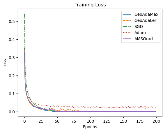
(a) Training loss

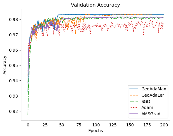
(b) Validation Accuracy

Figure 1: MNIST

6.2 CIFAR-10 Dataset

In our CIFAR-10 [7] experiment, the algorithms ran for 100 epochs on a network comprised of two convolutional layers with a pooling layer between, followed by three-dense layers and a ReLU activation function on all layers. The results of this experiment are shown in figure 2 and Table 2. Once again, we find that the early run performance of GeoAdaLer tends to be on par or better than other algorithms, consistently peaking above them in terms of validation accuracy. Its long run performance was only matched by Adam and GeoAdaMax. The consistent performance of GeoAdaLer in different situations lend credence to the geometric approach. Computational times are as follows - CPU: 500mins, GPU: 250mins.

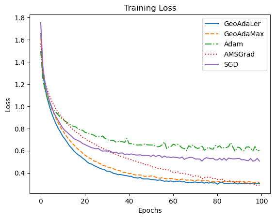
(a) Training loss

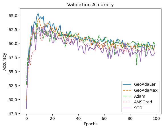
(b) Validation Accuracy

Figure 2: CIFAR

Table 1: MNIST Final Accuracy

Optimizer	Final Accuracy
GeoAdaLer	0.9832
GeoAdaMax	0.9829
Adam	0.9783
AMSGrad	0.9810
SGD	0.9815

Table 2: CIFAR Final Accuracy

Optimizer	Final Accuracy
GeoAdaLer	0.5970
GeoAdaMax	0.5958
Adam	0.5982
AMSGrad	0.5843
SGD	0.5837

7 Conclusion

In this paper, we investigate the adaptive stochastic gradient descent algorithm and propose a geometric approach where the normal vector to the tangent hyperplane plays a crucial role in providing curvature-like information. We call this approach GeoAdaLer, and we show that it is derived from a fundamental understanding of optimization geometry. We present theoretical proof for both deterministic and stochastic settings. Empirically, we find that GeoAdaLer is competitively comparable with other optimization techniques. Under certain conditions, it offers better performance and stability. GeoAdaLer provides a general geometric framework applicable to most, if not all, large-scale adaptive gradient-based optimization methods. We believe that this presents a significant step towards the development of interpretable machine learning algorithms through the lens of optimization.

Appendix A Deterministic Convergence Proof

Definition 1.

A differentiable function $f$ on $\mathbb{R}^{n}$ is said to be co-coercive if

$$\frac{1}{L}\|\nabla f(x)-\nabla f(y)\|^{2}\leq\langle\nabla f(x)-\nabla f(y),x-y\rangle,\text{ for all }x,y\in\mathbb{R}^{n}.$$ (13)

Lemma 1.

Let $\nabla f$ be Lipschitz continuous with constant $L>0$. Then $\frac{\nabla f}{\sqrt{\|\nabla f\|^{2}+1}}$ is Lipschitz continuous.

Proof.

Follows since $\frac{\nabla f}{\sqrt{\|\nabla f\|^{2}+1}}$ is a continuous function of $\nabla f$. ∎

Lemma 2 (Co-coercivity).

Let $\nabla f$ be Lipschitz and let $L_{G}$ be the Lipschitz constant for $\displaystyle\frac{\nabla f}{\sqrt{\|\nabla f\|^{2}+1}}$. Then the following co-coercivity property holds:

$$\frac{1}{L_{G}}\left\|\frac{\nabla f(x)}{\sqrt{\|\nabla f(x)\|^{2}+1}}-\frac{\nabla f(y)}{\sqrt{\|\nabla f(y)\|^{2}+1}}\right\|^{2}\leq\bigg{\langle}\frac{\nabla f(x)}{\sqrt{\|\nabla f(x)\|^{2}+1}}-\frac{\nabla f(y)}{\sqrt{\|\nabla f(y)\|^{2}+1}},x-y\bigg{\rangle}\$$ (14)

Lemma 3.

Suppose $\nabla f$ is Lipschitz continuous with parameter $L$, domain of $f$ is $\mathbb{R}^{n}$ and $f$ has a minimum at $x^{*}$. Then

$$\frac{1}{2L}\|\nabla f(z)\|^{2}\leq f(z)-f(x^{*})$$

Proof.

The proof relies on the following quadratic upper bound property

$$f(y) \leq f(z)+\langle\nabla f(z),y-z\rangle+\frac{L}{2}\|y-z\|^{2}\quad\text{for all }y,z\in\text{ dom}(f)$$ (15)

where dom$(f)$. the domain of $f$ is a convex set. i.e., taking infimum on both sides of 15 gives

$$f(x^{*})=\inf_{y}f(y) \leq\inf_{y}(f(z)+\langle\nabla f(z),y-z\rangle+\frac{L}{2}\|y-z\|^{2}$$

$$=\inf_{\|v\|=1}\inf_{t}\left(f(z)+t\langle\nabla f(z),v\rangle+\frac{Lt^{2}}{2}\right)$$

$$=\inf_{\|v\|=1}\left(f(z)-\frac{1}{2L}\langle\nabla f(z),v\rangle\right)$$

$$=f(z)-\frac{1}{2L}\|\nabla f(z)\|^{2}$$ (16)

Rearranging the terms in 16 gives the desired result. ∎

Proof.

For any $x$ and $y$, let

$$f_{x}(z)\coloneqq F(z)-\frac{\nabla f(x)^{T}z}{\sqrt{\|\nabla f(x)\|^{2}+1}},$$ (17)

$$f_{y}(z)\coloneqq F(z)-\frac{\nabla f(y)^{T}z}{\sqrt{\|\nabla f(y)\|^{2}+1}}$$ (18)

for some constant $a$ where $\displaystyle F(z)\coloneqq\int_{a}^{z}\frac{\nabla f(u)}{\sqrt{\|\nabla f(u)\|^{2}+1}}du$ is a scalar potential function for the vector field integrand. Notice that $F$ is well defined since the integrand is a conservative vector field. Also, F(z) is convex since the integrand is a monotone operator.

Thus, $f_{x}$ and $f_{y}$ are well defined and convex since the difference of a convex function and a linear function is convex. $f_{x}$ is minimized at $z=x$, thus evaluating $f_{x}$ at $y$ and $x$ and subtracting the results gives

$$F(y) -F(x)-\bigg{\langle}\frac{\nabla f(x)}{\sqrt{\|\nabla f(x)\|^{2}+1}},y-x\bigg{\rangle}$$

$$=f_{x}(y)-f_{x}(x)$$

$$\geq\frac{1}{2L_{G}}\|\nabla f_{x}(y)\|^{2}$$ (19)

$$=\frac{1}{2L_{G}}\bigg{\|}\frac{\nabla f(y)}{\sqrt{\|\nabla f(y)\|^{2}+1}}-\frac{\nabla f(x)}{\sqrt{\|\nabla f(x)\|^{2}+1}}\bigg{\|}^{2}$$ (20)

Equation 19 follows from Lemma 3 and equation 20 from taking the gradient of $f_{x}$ at $x$.

Similarly, $z=y$ minimizes $f_{y}$ and

$$F(x) -F(y)-\bigg{\langle}\frac{\nabla f(y)}{\sqrt{\|\nabla f(y)\|^{2}+1}},x-y\bigg{\rangle}$$

$$=f_{y}(x)-f_{y}(y)$$

$$\geq\frac{1}{2L_{G}}\|\nabla f_{y}(x)\|^{2}$$

$$=\frac{1}{2L_{G}}\bigg{\|}\frac{\nabla f(y)}{\sqrt{\|\nabla f(y)\|^{2}+1}}-\frac{\nabla f(x)}{\sqrt{\|\nabla f(x)\|^{2}+1}}\bigg{\|}^{2}$$ (21)

Adding the inequalities 20 and 21, we obtain

$$\frac{1}{L_{G}}\left\|\frac{\nabla f(x)}{\sqrt{\|\nabla f(x)\|^{2}+1}}-\frac{\nabla f(y)}{\sqrt{\|\nabla f(y)\|^{2}+1}}\right\|^{2} \leq\bigg{\langle}\frac{\nabla f(x)}{\sqrt{\|\nabla f(x)\|^{2}+1}}-\frac{\nabla f(y)}{\sqrt{\|\nabla f(y)\|^{2}+1}},x-y\bigg{\rangle}.$$

∎

Theorem 4.

Let $f:\mathbb{R}^{d}\to\mathbb{R}$ be continuous and $\nabla f$ Lipschitz continuous with $\gamma\leq\frac{1}{L}$ where $L$ is the Lipschitz constant for $\nabla f$. Assume $f$ attains an optimal value at $x^{*}=\arg\min_{x}f(x)$. Then $T$ defined in (9) is a contraction map with contraction parameter $\alpha=\sqrt{1+\gamma^{2}L_{G}^{2}-2\gamma\frac{L_{G}^{2}}{L}}$ where $L_{G}$ is the Lipschitz constant for $\displaystyle\frac{\nabla f}{\sqrt{\|\nabla f\|^{2}+1}}$ and $\|\cdot\|$ is the Euclidean norm in $\mathbb{R}^{n}$.

Proof.

It suffices to show that for some $\alpha\in[0,1)$,

$$\|Tx-Ty\|\leq\alpha\|x-y\|.$$ (22)

To this end, we compute as follows

$$\|Tx-Ty\|^{2} =\bigg{\|}x-\frac{\gamma\nabla f(x)}{\sqrt{\|\nabla f(x)\|^{2}+1}}-y+\frac{\gamma\nabla f(y)}{\sqrt{\|\nabla f(y)\|^{2}+1}}\bigg{\|}^{2}$$

$$=\bigg{\|}(x-y)-\gamma\left(\frac{\nabla f(x)}{\sqrt{\|\nabla f(x)\|^{2}+1}}-\frac{\nabla f(y)}{\sqrt{\|\nabla f(y)\|^{2}+1}}\bigg{)}\right\|^{2}$$

$$=\|x-y\|^{2}-2\gamma\left\langle x-y,\frac{\nabla f(x)}{\sqrt{\|\nabla f(x)\|^{2}+1}}-\frac{\nabla f(y)}{\sqrt{\|\nabla f(y)\|^{2}+1}}\right\rangle$$

$$+\gamma^{2}\bigg{\|}\frac{\nabla f(x)}{\sqrt{\|\nabla f(x)\|^{2}+1}}-\frac{\nabla f(y)}{\sqrt{\|\nabla f(y)\|^{2}+1}}\bigg{\|}^{2}$$

$$\leq\bigg{\|}x-y\bigg{\|}^{2}+\bigg{(}\gamma^{2}-\frac{2\gamma}{L_{G}}\bigg{)}\Bigg{\|}\frac{\nabla f(x)}{\sqrt{\|\nabla f(x)\|^{2}+1}}-\frac{\nabla f(y)}{\sqrt{\|\nabla f(y)\|^{2}+1}}\Bigg{\|}^{2}$$ (23)

$$\leq\|x-y\|^{2}+L_{G}^{2}\bigg{(}\gamma^{2}-\frac{2\gamma}{L_{G}}\bigg{)}\|x-y\|^{2}$$ (24)

$$\leq\bigg{(}1+\gamma^{2}L_{G}^{2}-\frac{2\,\gamma L_{G}^{2}}{L}\bigg{)}\|x-y\|^{2}$$ (25)

Inequality (23) follows from co-coercivity (see Lemma 2) while 24 follows from the continuity of $\displaystyle\frac{\nabla f}{\sqrt{\|\nabla f\|^{2}+1}}$ and the Lipschitz continuity of $\nabla f$. ∎

Appendix B Stochastic Convergence Proof

B.1 Important Lemmas and Definitions

In this section, we provide proof of convergence of our algorithm. To this end, we start with some definitions and lemmas necessary for the main theorem.

Definition 2.

A differentiable function $f:\mathbb{R}^{d}\to\mathbb{R}$ is convex if for all $x,y\in\mathbb{R}$,

$$f(y)\geq f(x)+\nabla f(x)^{T}(y-x).$$ (26)

For the rest of the paper, we make the following assumptions on the stochastic objective function $f_{t}:\mathbb{R}^{d}\to\mathbb{R}$ where the iteration counter $t\geq 1$.

Assumptions 1.

1. $f_{t}$ is convex for all $t$.

2. For all $t,f_{t}$ is differentiable.

3. For all $t$, there exists $G\geq 0$ such that $\|\nabla f_{t}(x)\|\leq D$ for all $x\in X\subseteq\mathbb{R}^{d}$ where $X$ is the feasible set.

4. $A\coloneqq\{x_{1},x_{2},\cdots\}$, the iterates generated by GeoAdaLer algorithm.

5. $x^{*}\coloneqq\arg\min_{x\in X}\sum_{t=1}^{T}f_{t}(x)$ exists and $\|x_{k}-x^{*}\|\leq D$ for all $x_{k}\in A$.

6. $\beta_{t}\coloneqq\beta\lambda^{t-1}$ where $\lambda\in(0,1),\beta\in[0,1)$.

Also, for notational convenience, we take $g_{t}=\nabla f_{t}(x_{t})$.

Lemma 4.

Under Assumptions 1, no. 3, the exponential moving average

$$m_{t}=\beta_{t}m_{t-1}+(1-\beta_{t})g_{t}$$ (27)

is bounded for all $t$.

Proof.

Iteratively expanding out $m_{t}$, we obtain

$$m_{t}=(1-\beta_{t})\sum_{i=1}^{t}\beta_{t}^{t-i+1}g_{i}.$$

Taking the Euclidean norm on both sides and using the boundedness of $g_{t}$ gives

$$\|m_{t}\| =\|(1-\beta_{t})\sum_{i=1}^{t}\beta_{t}^{t-i+1}g_{i}\|$$

$$\leq(1-\beta_{t})\sum_{i=1}^{t}\beta_{t}^{t-i+1}\|g_{i}\|$$

$$\leq(1-\beta_{t})G\sum_{i=1}^{t}\beta_{t}^{t-i+1}$$

$$=G(1-\beta_{t}^{t})\leq G$$

∎

Lemma 5.

Under Assumptions 1, no. 6, the following inequalities hold

1. $\displaystyle\frac{\beta_{t}}{1-\beta_{t}}\leq\frac{\beta}{1-\beta}$

2. $\displaystyle\frac{1}{1-\beta_{t}}\leq\frac{1}{1-\beta}$

3. $\displaystyle\sum_{t=1}^{T}\frac{\beta_{t}}{1-\beta_{t}}\leq\frac{\beta(1-\lambda^{T})}{(1-\beta)(1-\lambda)}$

for all $t$.

Proof.

1). For all $t,\lambda<1$ gives $\lambda^{t-1}<1$ so that $\frac{1}{\lambda^{1-t}}<1$. Thus

$$\frac{\beta_{t}}{1-\beta_{t}} =\frac{\beta\lambda^{t-1}}{1-\beta\lambda^{t-1}}=\frac{\beta}{\lambda^{1-t}-\beta}\leq\frac{\beta}{1-\beta}.$$

2). $\beta_{t}=\beta\lambda^{t-1}\leq\beta$ for all $t$ since $\lambda\in(0,1),\beta\in[0,1)$. So, $1-\beta\leq 1-\beta\lambda^{t-1}$ leads to $\displaystyle\frac{1}{1-\beta_{t}}\leq\frac{1}{1-\beta}$ as required.

3). By Lemma 5 no. 2, we have

$$\sum_{t=1}^{T}\frac{\beta_{t}}{1-\beta_{t}}\leq\sum_{t=1}^{T}\frac{\beta_{t}}{1-\beta}=\frac{\beta}{1-\beta}\sum_{t=1}^{T}\lambda^{t-1}=\frac{\beta(1-\lambda^{T})}{(1-\beta)(1-\lambda)}$$

∎

Lemma 6.

For all $t\geq 1$ and for all $T\geq t$, the following inequality holds

$$\sum_{t=1}^{T}\frac{1}{\sqrt{t}}\leq 1+\int_{1}^{T}\frac{1}{\sqrt{t}}dt$$ (28)

Proof trivially follows from the integral test for convergence of series and is also given in [1].

Lemma 7.

Under Assumptions 1, no. 1 and 2, the following inequality holds for all $t$

$$R(T)\leq\sum_{t=1}^{T}g_{t}\cdot(x_{t}-x^{*}).$$ (29)

Proof.

By converxity of $f_{t}$ for each $t$,

$$f_{t}(x^{*})-f_{t}(x_{t})\geq\nabla f_{t}(x_{t})\cdot(x^{*}-x_{t})$$

It then follows that

$$f_{t}(x_{t})-f_{t}(x^{*})\leq\nabla f_{t}(x_{t})\cdot(x_{t}-x^{*})=g_{t}\cdot(x_{t}-x^{*})$$

Hence, summing both sides from $t=1$ to $T$ gives the required result. ∎

Appendix C Proof of Theorem 3

From the update rule in Algorithm 2

$$x_{t+1}=x_{t}-\gamma_{t}\frac{m_{t}}{\sqrt{\|m_{t}\|^{2}+1}}.$$

Subtracting $x^{*}$ from both sides and taking norm squared results

$$\|x_{t+1}-x^{*}\|^{2} =|x_{t}-\gamma_{t}\frac{m_{t}}{\sqrt{\|m_{t}\|^{2}+1}}|^{2}$$

$$=\|x_{t}-x^{*}\|^{2}-\frac{2\gamma_{t}}{\sqrt{\|m_{t}\|^{2}+1}}m_{t}\cdot(x_{t}-x^{*})+\gamma_{t}^{2}\frac{\|m_{t}\|^{2}}{\|m_{t}\|^{2}+1}.$$

Substituting $m_{t}=\beta_{t}m_{t-1}+(1-\beta_{t})g_{t}$, we obtain

$$\|x_{t+1}-x^{*}\|^{2} =\begin{multlined}\|x_{t}-x^{*}\|^{2}-\frac{2\gamma_{t}}{\sqrt{\|m_{t}\|^{2}+1}}m_{t-1}\cdot(x_{t}-x^{*})\\ -\frac{2\gamma_{t}(1-\beta_{t})}{\sqrt{\|g_{t}\|^{2}+1}}g_{t}\cdot(x_{t}-x^{*})+\gamma_{t}^{2}\frac{\|m_{t}\|^{2}}{\|m_{t}\|^{2}+1}.\end{multlined}\|x_{t}-x^{*}\|^{2}-\frac{2\gamma_{t}}{\sqrt{\|m_{t}\|^{2}+1}}m_{t-1}\cdot(x_{t}-x^{*})\\ -\frac{2\gamma_{t}(1-\beta_{t})}{\sqrt{\|g_{t}\|^{2}+1}}g_{t}\cdot(x_{t}-x^{*})+\gamma_{t}^{2}\frac{\|m_{t}\|^{2}}{\|m_{t}\|^{2}+1}.$$

Rearrange to have $g_{t}\cdot(x_{t}-x^{*})$ on the left hand side:

$$g_{t}\cdot(x_{t}-x^{*}) =\begin{multlined}\frac{\sqrt{\|m_{t}\|^{2}+1}}{2\gamma_{t}(1-\beta_{t})}\left[\|x_{t}-x^{*}\|^{2}-\|x_{t+1}-x^{*}\|^{2}\right]-\frac{\beta_{t}}{1-\beta_{t}}m_{t-1}\cdot(x_{t}-x^{*})\\ +\frac{\gamma_{t}}{2(1-\beta_{t})}\frac{\|m_{t}\|^{2}}{\sqrt{\|m_{t}\|^{2}+1}}\end{multlined}\frac{\sqrt{\|m_{t}\|^{2}+1}}{2\gamma_{t}(1-\beta_{t})}\left[\|x_{t}-x^{*}\|^{2}-\|x_{t+1}-x^{*}\|^{2}\right]-\frac{\beta_{t}}{1-\beta_{t}}m_{t-1}\cdot(x_{t}-x^{*})\\ +\frac{\gamma_{t}}{2(1-\beta_{t})}\frac{\|m_{t}\|^{2}}{\sqrt{\|m_{t}\|^{2}+1}}$$ (32)

$$\leq\begin{multlined}\frac{\sqrt{\|m_{t}\|^{2}+1}}{2\gamma_{t}(1-\beta_{t})}\left[\|x_{t}-x^{*}\|^{2}-\|x_{t+1}-x^{*}\|^{2}\right]\\ +\frac{\beta_{t}}{1-\beta_{t}}\|m_{t-1}\|\|(x^{*}-x_{t})\|+\frac{\gamma_{t}\|m_{t}\|^{2}}{2(1-\beta_{t})}.\end{multlined}\frac{\sqrt{\|m_{t}\|^{2}+1}}{2\gamma_{t}(1-\beta_{t})}\left[\|x_{t}-x^{*}\|^{2}-\|x_{t+1}-x^{*}\|^{2}\right]\\ +\frac{\beta_{t}}{1-\beta_{t}}\|m_{t-1}\|\|(x^{*}-x_{t})\|+\frac{\gamma_{t}\|m_{t}\|^{2}}{2(1-\beta_{t})}.$$ (35)

where inequality 35 follows from the Cauchy-Schwartz inequality applied to the second term $-m_{t-1}\cdot(x_{t}-x^{*})=m_{t-1}\cdot(x^{*}-x_{t})$ and the fact that $\frac{\|m_{t}\|^{2}}{\sqrt{\|m_{t}\|^{2}+1}}\leq 1$ for all $t$.
Summing both sides from $t=1$ to $T$ and using Lemma 4 and Assumptions 1 no. 3 and 5, we further obtain

$$\sum_{t=1}^{T}g_{t}\cdot(x_{t}-x^{*}) \leq\begin{multlined}\sum_{t=1}^{T}\frac{\sqrt{G^{2}+1}}{2\gamma_{t}(1-\beta_{t})}\left[\|x_{t}-x^{*}\|^{2}-\|x_{t+1}-x^{*}\|^{2}\right]\\ +DG\sum_{t=1}^{T}\frac{\beta_{t}}{1-\beta_{t}}+G^{2}\sum_{t=1}^{T}\frac{\gamma_{t}}{2(1-\beta_{t})}\end{multlined}\sum_{t=1}^{T}\frac{\sqrt{G^{2}+1}}{2\gamma_{t}(1-\beta_{t})}\left[\|x_{t}-x^{*}\|^{2}-\|x_{t+1}-x^{*}\|^{2}\right]\\ +DG\sum_{t=1}^{T}\frac{\beta_{t}}{1-\beta_{t}}+G^{2}\sum_{t=1}^{T}\frac{\gamma_{t}}{2(1-\beta_{t})}$$ (37)

$$\leq\begin{multlined}\sum_{t=1}^{T}\frac{\sqrt{G^{2}+1}}{2\gamma_{t}(1-\beta_{t})}\left[\|x_{t}-x^{*}\|^{2}-\|x_{t+1}-x^{*}\|^{2}\right]\\ +\frac{DG\beta(1-\lambda^{T})}{(1-\beta)(1-\lambda)}+\frac{G^{2}}{2(1-\beta)}\sum_{t=1}^{T}\gamma_{t}.\end{multlined}\sum_{t=1}^{T}\frac{\sqrt{G^{2}+1}}{2\gamma_{t}(1-\beta_{t})}\left[\|x_{t}-x^{*}\|^{2}-\|x_{t+1}-x^{*}\|^{2}\right]\\ +\frac{DG\beta(1-\lambda^{T})}{(1-\beta)(1-\lambda)}+\frac{G^{2}}{2(1-\beta)}\sum_{t=1}^{T}\gamma_{t}.$$ (40)

where the last inequality follows from Assumptions 1 no. 3 and Lemma 5 no. 2 and 3.
By expanding the first term and and rewriting the what is left in compact form, we obtain

$$\sum_{t=1}^{T}\frac{1}{\gamma_{t}(1-\beta_{t})}\left[\|x_{t}-x^{*}\|^{2}-\|x_{t+1}-x^{*}\|^{2}\right] =\begin{multlined}\frac{1}{\gamma_{1}(1-\beta_{1})}\|x_{1}-x^{*}\|^{2}-\frac{1}{\gamma_{T}(1-\beta_{T})}\|x_{T+1}-x^{*}\|^{2}\\ +\sum_{t=2}^{T}\left(\frac{1}{\gamma_{t}(1-\beta_{t})}-\frac{1}{\gamma_{t-1}(1-\beta_{t-1})}\right)\|x_{t}-x^{*}\|^{2}\end{multlined}\frac{1}{\gamma_{1}(1-\beta_{1})}\|x_{1}-x^{*}\|^{2}-\frac{1}{\gamma_{T}(1-\beta_{T})}\|x_{T+1}-x^{*}\|^{2}\\ +\sum_{t=2}^{T}\left(\frac{1}{\gamma_{t}(1-\beta_{t})}-\frac{1}{\gamma_{t-1}(1-\beta_{t-1})}\right)\|x_{t}-x^{*}\|^{2}$$

$$\leq\begin{multlined}\frac{\|x_{1}-x^{*}\|^{2}}{\gamma_{1}(1-\beta_{1})}\\ +\sum_{t=1}^{T}\left(\frac{1}{\gamma_{t}(1-\beta_{t})}-\frac{1}{\gamma_{t-1}(1-\beta_{t-1})}\right)\|x_{t}-x^{*}\|^{2}.\end{multlined}\frac{\|x_{1}-x^{*}\|^{2}}{\gamma_{1}(1-\beta_{1})}\\ +\sum_{t=1}^{T}\left(\frac{1}{\gamma_{t}(1-\beta_{t})}-\frac{1}{\gamma_{t-1}(1-\beta_{t-1})}\right)\|x_{t}-x^{*}\|^{2}.$$

where the last inequality follows from dropping the second term. By the Assumptions 1 no. 5, it further simplifies to

$$\sum_{t=1}^{T}\frac{1}{\gamma_{t}(1-\beta_{t})}\left[\|x_{t}-x^{*}\|^{2}-\|x_{t+1}-x^{*}\|^{2}\right] \leq\frac{D^{2}}{\gamma_{1}(1-\beta_{1})}+D^{2}\sum_{t=2}^{T}\left(\frac{1}{\gamma_{t}(1-\beta_{t})}-\frac{1}{\gamma_{t-1}(1-\beta_{t-1})}\right)$$

$$=\frac{D^{2}}{\gamma_{1}(1-\beta_{1})}-\frac{D^{2}}{\gamma_{1}(1-\beta_{1})}+\frac{D^{2}}{\gamma_{T}(1-\beta_{T})}$$

$$=\frac{D^{2}}{\gamma_{T}(1-\beta_{T})}.$$

From Lemma 5 we have.

$$\sum_{t=1}^{T}\frac{1}{\gamma_{t}(1-\beta_{t})}\left[\|x_{t}-x^{*}\|^{2}-\|x_{t+1}-x^{*}\|^{2}\right]\leq\frac{D^{2}}{\gamma_{T}(1-\beta)}.$$

Therefore equation 40 become:

$$\sum_{t=1}^{T}g_{t}\cdot(x_{t}-x^{*}) \leq\frac{D^{2}\sqrt{G^{2}+1}}{\gamma_{T}(1-\beta_{T})}+\frac{DG\beta(1-\lambda^{T})}{(1-\beta)(1-\lambda)}+\frac{G^{2}}{2(1-\beta)}\sum_{t=1}^{T}\gamma_{t}.$$ (41)

Assuming $\gamma_{t}=\frac{1}{\sqrt{t}}$ we further obtain:

$$\sum_{t=1}^{T}g_{t}\cdot(x_{t}-x^{*}) \leq\frac{\sqrt{T}D^{2}\sqrt{G^{2}+1}}{(1-\beta_{T})}+\frac{DG\beta(1-\lambda^{T})}{(1-\beta)(1-\lambda)}+\frac{G^{2}}{2(1-\beta)}\sum_{t=1}^{T}\frac{1}{\sqrt{t}}$$ (42)

$$\leq\frac{\sqrt{T}D^{2}\sqrt{G^{2}+1}}{(1-\beta_{T})}+\frac{DG\beta(1-\lambda^{T})}{(1-\beta)(1-\lambda)}+\frac{G^{2}(2T-1)}{2(1-\beta)}.$$ (43)

Equation 43 follows from Lemma 6 and so our regret is bounded above by:

$$R(T)\leq\frac{\sqrt{T}D^{2}\sqrt{G^{2}+1}}{(1-\beta_{T})}+\frac{DG\beta(1-\lambda^{T})}{(1-\beta)(1-\lambda)}+\frac{G^{2}(2T-1)}{2(1-\beta)}.$$

Appendix D Datasets

MNIST: The MNIST database of handwritten digits. Licensed under the Creative Commons Attribution 4.0 License.[9]

CIFAR-10: The CIFAR-10 dataset consists of 60000 32x32 colour images in 10 classes, with 6000 images per class. There are 50000 training images and 10000 test images. Licensed under the Creative Commons Attribution 4.0 License[6]

References

[1]Sebastian Bock, Josef Goppold and Martin Weiß
“An improvement of the convergence proof of the ADAM-Optimizer”
In arXiv preprint arXiv:1804.10587, 2018
[2]Nicolo Cesa-Bianchi, Alex Conconi and Claudio Gentile
“On the generalization ability of on-line learning algorithms”
In IEEE Transactions on Information Theory50.9IEEE, 2004, pp. 2050–2057
[3]John Duchi, Elad Hazan and Yoram Singer
“Adaptive subgradient methods for online learning and stochastic optimization.”
In Journal of machine learning research12.7, 2011
[4]Geoffrey Hinton, Nitish Srivastava and Kevin Swersky
“Neural networks for machine learning lecture 6a overview of mini-batch gradient descent”
In Cited on14.8, 2012, pp. 2
[5]Diederik P Kingma and Jimmy Ba
“Adam: A method for stochastic optimization”
In arXiv preprint arXiv:1412.6980, 2014
[6]Alex Krizhevsky
“Learning multiple layers of features from tiny images”, 2009
[8]Y. Lecun, L. Bottou, Y. Bengio and P. Haffner
“Gradient-based learning applied to document recognition”
In Proceedings of the IEEE86.11, 1998, pp. 2278–2324
DOI: 10.1109/5.726791
[9]Yann LeCun, Corinna Cortes and CJ Burges
“MNIST handwritten digit database”
In ATT Labs [Online]. Available: http://yann.lecun.com/exdb/mnist2, 2010
[10]Haochuan Li, Alexander Rakhlin and Ali Jadbabaie
“Convergence of Adam under relaxed assumptions”
In Advances in Neural Information Processing Systems36, 2024
[11]Kamil Nar and S Shankar Sastry
“Step Size Matters in Deep Learning”, 2011
[12]Sashank J Reddi, Satyen Kale and Sanjiv Kumar
“On the convergence of adam and beyond”
In arXiv preprint arXiv:1904.09237, 2019
[14]Naichen Shi and Dawei Li
“Rmsprop converges with proper hyperparameter”
In International conference on learning representation, 2021
[15]T. Tieleman
“Lecture 6.5-rmsprop: Divide the Gradient by a Running Average of Its Recent Magnitude”
In COURSERA: Neural Networks for Machine Learning4.2, 2012, pp. 26
URL: https://cir.nii.ac.jp/crid/1370017282431050757
[17]Matthew D Zeiler
“Adadelta: an adaptive learning rate method”
In arXiv preprint arXiv:1212.5701, 2012
[18]Yushun Zhang et al.
“Adam can converge without any modification on update rules”
In Advances in neural information processing systems35, 2022, pp. 28386–28399
[19]Martin Zinkevich
“Online convex programming and generalized infinitesimal gradient ascent”
In Proceedings of the 20th international conference on machine learning (icml-03), 2003, pp. 928–936