Conformal Robust Control of Linear Systems

Abstract

End-to-end engineering design pipelines, in which designs are evaluated using concurrently defined optimal controllers, are becoming increasingly common in practice. To discover designs that perform well even under the misspecification of system dynamics, such end-to-end pipelines have now begun evaluating designs with a robust control objective in place of the nominal optimal control setup. Current approaches of specifying such robust control subproblems, however, rely on hand specification of perturbations anticipated to be present upon deployment or margin methods that ignore problem structure, resulting in a lack of theoretical guarantees and overly conservative empirical performance. We, instead, propose a novel methodology for LQR systems that leverages conformal prediction to specify such uncertainty regions in a data-driven fashion. Such regions have distribution-free coverage guarantees on the true system dynamics, in turn allowing for a probabilistic characterization of the regret of the resulting robust controller. We then demonstrate that such a controller can be efficiently produced via a novel policy gradient method that has convergence guarantees. We finally demonstrate the superior empirical performance of our method over alternate robust control specifications in a collection of engineering control systems, specifically for airfoils and a load-positioning system.

1 Introduction

Seeking control over a family of dynamical systems is a problem often encountered in science and engineering [1, 2, 3]. One particularly prevalent application of this is in integrated control and design settings, known as control co-design (CCD) [4]. Traditional engineering design workflows operate sequentially, first proposing a design and subsequently designing a corresponding controller [5, 6]. Such workflows, however, sacrifice the improved optimality possible in coupling the two, hence increasing interest in leveraging end-to-end co-control design pipelines [7, 8].

Initial works in CCD studied optimal design assuming perfectly specified, deterministic system dynamics [9, 10, 11, 12]. Given the expanding use of CCD, such assumptions have become overly restrictive, resulting in interest in robust extensions of the CCD formulation, referred to as uncertain CCD (UCCD) [13, 14, 15]. Such uncertainty can arise from many sources in the design process, such as noise in the control channels, uncertainties in the design parameters due to manufacturing imperfections, or unmodeled components of the system dynamics. In addition, the nature of the UCCD problem specification differs depending on the risk tolerance in the downstream engineering application of interest. For instance, in risk-neutral settings, stochastic problem specifications are often appropriate [16, 17, 18], whereas in more risk-averse settings probabilistic [19, 20, 21] or worst-case problem specifications [22, 23, 24] are preferred.

We focus herein on the worst-case robust UCCD formulation (WCR-UCCD), specifically concentrating on uncertainties arising from dynamics misspecification. As in other worst-case problem formulations, WCR-UCCD requires the specification of a compact uncertainty region. Existing methods of specification, however, tend to be ad-hoc, relying on domain knowledge. Such methods, thus, fail to provide any theoretical characterization of the robust solution as it relates to the selection of this uncertainty set, rendering its choice in practice difficult and often resulting in suboptimal designs with overly conservative controllers [16].

Towards this end, we focus herein on providing a principled distribution-free specification of the robust control subproblem in WCR-UCCD and an associated solution method with convergence guarantees. One special case of interest in UCCD is in the setting of linear quadratic regulators (LQRs), where the underlying system dynamics take on a linear structure [25, 26, 27]. LQR systems are of broad interest both due to their analytic tractability and widespread applicability to practical engineering systems, especially due to their extensibility to nonlinear systems via Koopman operators [28, 29, 30]. We, therefore, propose a method for specifying the LQR WCR-UCCD robust control subproblem that lends itself to efficient solution by leveraging conformal prediction on observed design information. A comparable integration with conformal prediction was recently studied in [31], there applied to the predict-then-optimize setting. Unlike their setting, however, the application of conformal prediction to control has technical complications related to the stability of controllers under model uncertainty. Our contributions are as follows:

• Providing a framework to define robust LQR control problems with distribution-free probabilistic regret guarantees, across deterministic or stochastic and discrete- or continuous-time dynamics over infinite or finite time horizons.

• Providing an efficient policy gradient algorithm for obtaining the optimal robust controller with convergence guarantees proven via gradient dominance.

• Extending the line of conformalized predict-then-optimize to cases where calibration data is observed with noise and where the domains of both the maximization and minimization components of the robust formulation depend on the conformalized predictor.

2 Background

2.1 Conformal Prediction

Conformal prediction is a principled, distribution-free approach of uncertainty quantification [32, 33]. “Split conformal,” the most common variant of conformal prediction, is used as a wrapper around black-box predictors $\widehat{f}:\mathcal{X}\rightarrow\mathcal{Y}$ such that prediction regions $\mathcal{C}(x)$ are returned in place of the typical point predictions $\widehat{f}(x)$. Prediction regions $\mathcal{C}(x)$ are specifically sought to have coverage guarantees on the true $y:=f(x)$. That is, for some prespecified $\alpha$, we wish to have $\mathcal{P}_{X,Y}(Y\in\mathcal{C}(X))\geq 1-\alpha$.

To achieve this, split conformal partitions the overall dataset $\mathcal{D}$ into two subsets, $\mathcal{D}_{T}\cup\mathcal{D}_{C}$, respectively the training and calibration datasets. The training dataset is used in the standard manner to fit $\widehat{f}$. After fitting $\widehat{f}$, the calibration set is used to measure the anticipated “prediction error” for future test points. Formally, this error is quantified via a score function $s(x,y)$, which generalizes the classical notion of a residual. In particular, scores are evaluated on the calibration dataset to define $\mathcal{S}:=\{s(x,y)\mid(x,y)\in\mathcal{D}_{C}\}$. Denoting the $\lceil(|\mathcal{D}_{C}|+1)(1-\alpha)\rceil/|\mathcal{D}_{C}|$ empirical quantile of $\mathcal{S}$ as $\widehat{q}$, conformal prediction defines $\mathcal{C}(x)$ to be $\{y\mid s(x,y)\leq\widehat{q}\}$. Such $\mathcal{C}(x)$ satisfies the aforementioned coverage guarantees under the exchangeability of future test points $(x^{\prime},y^{\prime})$ with points from $\mathcal{D}_{C}$.

While the coverage guarantee holds for any arbitrarily specified score function, the conservatism of the resulting prediction region, known as the procedure’s “predictive efficiency,” is dependent on its choice [33]. The practical objective of conformal prediction, therefore, is to define score functions that retain coverage while minimizing the resulting prediction region size.

2.2 Predict-Then-Optimize

We present a summary of the application of conformal prediction to predict-then-optimize problems, specifically from [31]. Predict-then-optimize problems are nominally formulated as

$$w^{*}(x):=\min_{w\in\mathcal{W}} \mathbb{E}[f(w,C)\mid X],$$ (1)

where $w$ are decision variables, $C$ an unknown cost parameter, $x$ observed contextual variables, $\mathcal{W}$ a compact feasible region, and $f(w,c)$ an objective function that is convex-concave and $L$-Lipschitz in $c$ for any fixed $w$. The nominal approach defines a predictor $\widehat{g}:\mathcal{X}\rightarrow\mathcal{C}$, where the prediction $\widehat{c}:=\widehat{g}(x)$ is directly leveraged in the downstream optimization task, i.e. taking $w^{*}:=\min_{w}f(w,\widehat{c})$.

Such an approach, however, is inappropriate in safety-critical settings, given that the predictor function $\widehat{g}$ will likely be misspecified and, thus, may result in suboptimal decisions under the true cost parameter, which we denote as $c$. For this reason, robust alternatives to the formulation given by Equation 1 have become of interest. We focus on the formulation posited in [31], which extended the line of work begun in [34, 35, 36]. In particular, they studied

$$\begin{gathered}w^{*}(x):=\min_{w}\max_{\widehat{c}\in\mathcal{U}(x)}\quad f(w,\widehat{c})\quad\textrm{s.t.}\quad\mathcal{P}_{X,C}(C\in\mathcal{U}(x))\geq 1-\alpha,\\ \end{gathered}$$ (2)

where $\mathcal{U}:\mathcal{X}\rightarrow\mathcal{F}$ is a uncertainty region predictor, with $\mathcal{F}$ being the $\sigma$-field of $\mathcal{C}$. Works in this field typically focus on both theoretically characterizing and empirically studying the resulting suboptimality gap, defined as $\Delta(x,c):=\min_{w}\max_{\widehat{c}\in\mathcal{U}(x)}f(w,\widehat{c})-\min_{w}f(w,c)$. For instance, in [31], $\mathcal{U}(x)$ was specifically constructed via conformal prediction to provide probabilistic guarantees; that is, by taking $\mathcal{U}(x):=\mathcal{C}(x)$ to be the prediction region produced by conformalizing the predictor $\widehat{g}$, they demonstrated $\mathcal{P}_{X,C}\left(0\leq\Delta(X,C)\leq L\mathrm{\ diam}(\mathcal{U}(X))\right)\geq 1-\alpha$.

2.3 Linear Quadratic Regulators and Control Co-Design

The field of control has a long history in engineering physics and robotics [37]. The most heavily studied specific control setup is the linear quadratic regulator (LQR), where dynamics of the underlying state $x$ are assumed to have a linear form, consisting of both an autonomous and controlled component, namely $\dot{x}=Ax+Bu+w$, where $u$ are the control inputs and $w\sim\mathcal{D}_{w}$ the noise. Optimal control is then posed as a constrained optimization problem, with the objective $J(u)$ consisting of a term related to the deviation from a target state and another related to the control input. Under linear dynamics and quadratic cost, it is well-known that the optimal controller has a linear feedback form, namely $u^{*}(x)=-K^{*}x$ where $K^{*}$ is known as the “optimal gain matrix.” For this reason, optimization is sought over gain matrices $K$ rather than a more general function space of controllers:

$$K^{*}(A,B):=\operatorname*{arg\,min}_{K\in\mathcal{K}(A,B)}\mathbb{E}[J(K,A,B)]\mathrm{\ \ where}\quad J(K,A,B):=\int_{0}^{\infty}(x^{\top}Qx+(Kx)^{\top}R(Kx))dt$$

$$\textrm{s.t.}\quad\dot{x}=(A-BK)x+w\quad\quad\mathcal{K}(A,B):=\{K:\mathrm{Re}(\lambda_{i}(A-BK))<0\quad\forall i\}$$ (3)

$\mathcal{K}(A,B)$ is known as the set of “stabilizing controllers” for the $A,B$ system dynamics. Variations, where the integral is replaced by a discretized sum or where the cost is only considered to some finite $T$ time horizon, are also of interest in some settings. Solving this problem is typically done either by solving the algebraic Ricatti equation [38] or via policy gradient techniques [39].

We are interested herein in the robust control problem subproblem specification in the context of uncertain co-control design. We briefly summarize the relevant pieces of UCCD herein; for a full survey, refer to [13]. Worst-case robust UCCD for LQR with dynamics misspecification solves:

$$\begin{gathered}\min_{K,\theta}\max_{\widehat{A}\in\mathcal{A}(\theta),\widehat{B}\in\mathcal{B}(\theta)}\mathbb{E}[o(K,\widehat{A},\widehat{B},\theta)]\qquad\textrm{s.t.}\quad\dot{x}=\widehat{A}x+\widehat{B}u+w,\end{gathered}$$ (4)

where $\theta$ is a design parameter, $\mathcal{A}(\theta)$ and $\mathcal{B}(\theta)$ are respectively uncertainty sets of the dynamics for such a design, and $o$ is the objective function of interest. Often, the objective takes a decomposable form, namely with one term relating to system control and the other depending on the design parameter, i.e. $o(K,A,B,\theta):=\ell(\theta)+J(K,A(\theta),B(\theta))$ [40, 25]. One of the most commonly applied solution techniques of Equation 4 is via bilevel optimization, in which an outer optimization loop is performed over design parameters and an inner one over control parameters [41, 42]. For this reason, the specification of the robust control subproblem can be studied independently of the outer design optimization, as we do herein.

2.4 Related Works

Robust control broadly seeks to define a controller that performs well under model misspecification while minimizing regret under the true system dynamics, $\mathcal{R}(K,A,B):=\mathbb{E}[J(K,A,B)-J(K^{*}(A,B),A,B)]$, where the expectation is over randomness in the system dynamics, i.e. if $w\neq 0$ in Equation 3 [43]. We explicitly note $A,B$ in the regret notation to emphasize that, while the controller $K$ is often defined using estimated system dynamics $\widehat{A},\widehat{B}$, the final evaluation is an expectation over the true $A,B$ dynamics.

Much of robust control traditionally focuses on feedback control, where model misspecification is corrected adaptively over trajectories [13, 44, 45]. Such methods, however, cannot be leveraged in control co-design, since the goal is to identify an optimal robust controller prior to deploying a design. Importantly, however, we note that trajectories are often observed for a subset of the design space, given that engineering design is often performed in an iterative fashion, with physical tests being conducted alongside in-silico optimization; when present, CCD methods often employ such experimental data to learn a probabilistic surrogate dynamics model over the design space $q(X\mid\theta)$ to specify a stochastic UCCD formulation [46, 47, 48].

One classical specification of robust LQR control that lends itself to the trajectory-free setting is LQR with multiplicative noise (LQRm), where the controller is defined as:

$$\begin{gathered}\operatorname*{arg\,min}_{K}\mathbb{E}_{\{\delta_{i}\},\{\gamma_{i}\}}[J(K,A,B)]\quad\textrm{s.t.\ }\dot{x}:=\left(A+\sum_{i=1}^{p}\delta_{i}A_{i}\right)x+\left(B+\sum_{i=1}^{q}\gamma_{i}B_{i}\right)u+w,\end{gathered}$$ (5)

where $\{A_{i}\}$ and $\{B_{i}\}$ are specified explicitly a priori and the distributions of $\{\delta_{i}\}\sim\mathcal{D}_{\delta}$ and $\{\gamma_{i}\}\sim\mathcal{D}_{\gamma}$ similarly specified upfront. Such specification can either be performed manually via domain knowledge or in an automated fashion using margin approaches. Briefly, margin methods specify $\{\delta_{i}\}$ and $\{\gamma_{i}\}$ by finding those $\{\delta_{i}\}$ and $\{\gamma_{i}\}$ that result in borderline-stable dynamics when paired with the corresponding $(\{A_{i}\},\{B_{i}\})$ and some choice of controller: the particular controller varies across margin strategies. A full description of the margin methods considered in our experiments is given in Appendix I. Such methods, however, ignore the structural nature of the misspecification in the predictions of dynamics, in turn either sacrificing coverage or producing overly conservative robust controllers.

3 Conformalized Predict-Then-Control

We now introduce an approach to define and solve a robust LQR problem with probabilistic guarantees. We specifically discuss the problem formulation in Section 3.1 and the consequences resulting from this particular formulation on the downstream controllers in Section 3.3 and Section 3.4. We then provide an algorithm to extract this controller with convergence guarantees in Section 3.5. We finally demonstrate the improvement in average regret over non-data-driven approaches in Section 4.

3.1 Problem Formulation

For the presentation below, we use the following notational conventions. Assume $x_{t}\in\mathbb{R}^{n}$, $u_{t}\in\mathbb{R}^{m}$, $A\in\mathbb{R}^{n\times n}$, $B\in\mathbb{R}^{n\times m}$, and $C$ denotes the full dynamics matrix $C=[A,B]\in\mathbb{R}^{n\times(n+m)}$. We additionally assume a linear control scheme, namely $u_{t}=-Kx_{t}$ for some gain matrix $K$. Additionally, denote $W:=\begin{bmatrix}I&0\\ 0&-K\end{bmatrix}$, such that $CW=A-BK$. As discussed in Section 2.4, we assume a dataset of designs and associated trajectories are observed, that is, a dataset $\mathcal{D}$ of the form $\mathcal{D}=\{\theta_{i},\{(x_{i}^{(t)},u_{i}^{(t)})\}_{t=1}^{T}\}_{i=1}^{N}$, where $N$ is the number of samples and $T$ the time horizon. Notably, such trajectories $\{(x_{i}^{(t)},u_{i}^{(t)})\}_{t=1}^{T}$ need not arise from a fixed controller $K$ across designs $\{\theta_{i}\}$.

As discussed in Section 2.4, we are interested in studying a risk-sensitive formulation of LQR, namely seeking to define a controller that solves:

$$K^{*}_{\mathrm{rob}}(\mathcal{U}(\theta)):=\operatorname*{arg\,min}_{K\in\mathcal{K}(\mathcal{U}(\theta))}\max_{[\widehat{A},\widehat{B}]:=\widehat{C}\in\mathcal{U}(\theta)}\mathbb{E}[J(K,\widehat{A},\widehat{B})],$$ (6)

$$\textrm{s.t.}\quad\dot{x}=\widehat{A}x+\widehat{B}u+w\qquad\mathcal{P}_{\Theta,C}(C\in\mathcal{U}(\Theta))\geq 1-\alpha,$$

where $J$ is the objective function particular to the setting of interest, differing between infinite and finite time horizons and continuous and discrete time dynamics and $\mathcal{U}(\theta)$ is an uncertainty set over dynamics. Notably, the notion of stabilizing controllers as specified in Equation 3 must be generalized in the robust formulation, since the nominal formulation is for a specific $C$. We, thus, consider those controllers that stabilize the entire uncertainty set. Formally, we consider $\mathcal{K}(\mathcal{U}(\theta)):=\bigcap_{\widehat{C}\in\mathcal{U}(\theta)}\mathcal{K}(\widehat{C})$, where $\mathcal{K}(\widehat{C})$ is Equation 3 evaluated for a particular $\widehat{A},\widehat{B}$.

3.2 Score Function

From the trajectories observed in $\mathcal{D}$, we can perform system identification using dynamic mode decomposition with control (DMDc) to determine the corresponding $(\widetilde{A}_{i},\widetilde{B}_{i})$ [49]. With this, we obtain a final dynamics dataset $\widetilde{\mathcal{D}}=\{\theta_{i},\widetilde{C}_{i}\}_{i=1}^{N}$, which we then leverage in the standard manner of split conformal prediction. That is, we split $\widetilde{\mathcal{D}}=\widetilde{\mathcal{D}}_{\mathcal{T}}\cup\widetilde{\mathcal{D}}_{\mathcal{C}}$, the former of which we use to train a system parameters predictor $\widehat{C}:=f(\theta)$. Notably, leveraging split conformal in this setting has the additional complication that the ground truth used, namely in $\widetilde{\mathcal{D}}_{\mathcal{C}}$, is itself an estimate $\widetilde{C}$ even though coverage is sought on $C$ directly. We assume for this initial discussion that for a fixed coverage level $\alpha$, we can obtain prediction regions with the desired coverage, satisfying $\mathcal{P}_{\Theta,C}(C\in\mathcal{U}(\Theta))\geq 1-\alpha$, using $\widetilde{\mathcal{D}}_{\mathcal{C}}$. The treatment of this additional gap between $\widetilde{C}$ and $C$ is discussed in Section 3.4.

We take the score to be a matrix-norm residual, namely: $s(\theta,C)=||f(\theta)-C||_{2}$, where $||\cdot||_{2}$ is the matrix operator norm, i.e. $||A||_{2}=\sigma_{\mathrm{max}}(A)$, from which the resulting prediction regions take on the form of $\mathcal{B}_{\widehat{q}}(f(\theta))$, namely a ball of radius $\widehat{q}$, the conformal quantile, under the $||\cdot||_{2}$ metric. We note that, in place of this simple matrix difference, another choice of norm or the GPCP score formulation of [31] could also be leveraged in our framework with minimal modification, the latter desirable if a generative model $q(C\mid\Theta)$ is defined in place of $f(\theta)$. However, in this context, the additional expressive power of a generative model is not useful, as the mapping between design parameters $\theta$ and $A,B$ often takes a unimodal form. This was true classically, where a deterministic map was parametrically given by physics, and remains true of data-driven surrogates in UCCD, highlighted by the use of neural-based point predictor surrogates [50, 51].

3.3 Coverage Guarantee Consequences

We now wish to characterize the regret induced through the introduction of robustness across LQR setups, that is $\mathcal{R}(\theta,C):=\mathbb{E}[J(K^{*}_{\mathrm{rob}}(\mathcal{U}(\theta)),C)-J(K^{*}(C),C)]$ , where the randomness is over stochastics in the true system dynamics $C:=[A,B]$ and in the $\mathcal{P}(C\mid\theta)$ map. Qualitatively, the regret characterizations provided below demonstrate that, across system conditions, the robust controller produces an upper bound to the value of the nominal control problem whose looseness decreases monotonically with the size of the prediction regions. Thus, users should seek to produce prediction regions that are as small as possible while providing coverage to produce informative upper bounds on the nominal optimal value. Notably, the problem in our setting, as formulated in Equation 6, has the additional complication not present in [31] that the domain of the minimization is also a function of $\mathcal{U}(\theta)$ rather than solely that of the maximization.

We state the results for the continuous, infinite time horizon case with both deterministic and stochastic dynamics below. Notably, the deterministic and stochastic cases are both stated below, as the qualitative nature of the assumptions differs, with the latter requiring an assumption on the discounted nature of $Q(t)$ and $R(t)$, while the former is fully compatible with non-discounted rewards. Further, the statements and complete proofs for discrete-time dynamics, finite time horizons, and combinations thereof are provided in Appendix B, Appendix C, Appendix D, and Appendix E.

Theorem 3.1.

Let $J(K,C)$ be the infinite horizon, continuous-time, deterministic analog of that defined in Equation 3, i.e. $J(K,C):=\int_{0}^{\infty}(x(t)^{\top}(Q+K^{\top}RK)x(t))dt$ for $w=0$. Assume that for any fixed $\theta$, $K\in\mathcal{K}(\mathcal{U}(\theta))$, and $C\in\mathcal{U}(\theta)$, $D(K):=\sqrt{n}||Q+K^{\top}RK||_{\infty}||x_{0}||_{\infty}^{2}||W||_{2}<\infty$. Assume further that $\mathcal{P}_{\Theta,C}(C\in\mathcal{U}(\Theta))\geq 1-\alpha$. Then, there is a function $g:\Omega(\Theta)\rightarrow\mathbb{R}$ such that $\Omega_{1}\subset\Omega_{2}\implies g(\Omega_{1})\leq g(\Omega_{2})$ that satisfies:

$$\mathcal{P}_{\Theta,C}\left(0\leq\mathcal{R}(\Theta,C)\leq g(\mathcal{U}(\Theta))\right)\geq 1-\alpha.$$ (7)

Theorem 3.2.

Let $J(K,C)$ be the infinite horizon, continuous-time, stochastic analog of that defined in Equation 3, i.e. $J(K,C):=\mathbb{E}\left[\int_{0}^{\infty}(x(t)^{\top}(Q(t)+K^{\top}R(t)K)x(t))dt\right]$ with $w(t)$ a white noise process with spectral density $\Sigma$. Assume that for any fixed $\theta$, $K\in\mathcal{K}(\mathcal{U}(\theta))$, and $C\in\mathcal{U}(\theta)$: (1) there exist constants $\alpha_{1},\beta_{1}>0$ such that $||Q(t)+K^{\top}R(t)K||\leq\beta_{1}e^{-\alpha_{1}t}$ and $\min_{C}(2\alpha_{2}(C)+\alpha_{1})>0$ where $\alpha_{2}(C):=\max_{K\in\mathcal{K}(C)}(-\max_{i}\mathrm{Re}(\lambda_{i}(CW)))$ and (2) $D_{1}(K):=\max_{t}\sqrt{n}||Q(t)+K^{\top}R(t)K||_{\infty}||x_{0}||_{\infty}^{2}||W||_{2}<\infty$ and $D_{2}(K):=||\Sigma||_{2}||W||_{2}<\infty$. Assume further that $\mathcal{P}_{\Theta,C}(C\in\mathcal{U}(\Theta))\geq 1-\alpha$. Then, there is a function $g:\Omega(\Theta)\rightarrow\mathbb{R}$ such that $\Omega_{1}\subset\Omega_{2}\implies g(\Omega_{1})\leq g(\Omega_{2})$ that satisfies:

$$\mathcal{P}_{\Theta,C}\left(0\leq\mathcal{R}(\Theta,C)\leq g(\mathcal{U}(\Theta))\right)\geq 1-\alpha.$$ (8)

3.4 Ambiguous Ground Truth

We now discuss the complication of obtaining coverage guarantees on $C$ despite only observing estimates $\widetilde{C}=C+\epsilon$ in the dataset. Intuitively, we show that if, for all $\theta$, the density $\mathcal{P}(C\mid\theta)$ peaks in $\mathcal{U}(\theta)$, we retain marginal coverage guarantees. If $\mathcal{P}(C\mid\theta)$ is unimodal and radially symmetric about its mode, this condition is satisfied so long as $\mathcal{U}(\theta)$ captures the mode. As mentioned, the map between design parameters $\theta$ and $A,B$ is often unimodal, making such a structural assumption reasonable. $\mathcal{U}(\theta)$ capturing the mode is also a weak assumption assuming a zero-centered distribution for $\epsilon$, since it then amounts to capturing the mode of $\mathcal{P}(\widetilde{C}\mid\theta)$, which holds for any sufficiently accurate predictor. We empirically demonstrate that such assumptions hold and, thus, that the coverage guarantees are retained for problems of interest in Section 4. This theorem is a multivariate extension of Theorem A.5 from [52], with the full proof deferred to Appendix F.

Theorem 3.3.

Let $\widetilde{C}=C+\epsilon$ where $\text{vec}(\epsilon)\sim\mathcal{N}(0,\Sigma)$. Assume $\mathcal{U}(\theta)=\{C^{\prime}\mid||f(\theta)-C^{\prime}||_{2}\leq\widehat{q}\}$ satisfies $\mathcal{P}_{\Theta,\widetilde{C}}(\widetilde{C}\in\mathcal{U}(\Theta))\geq 1-\alpha$. If for any $\theta$, $\mathcal{P}(C\mid\theta)$ peaks in $\mathcal{U}(\theta)$, that is for any $\delta>0$, $\mathcal{P}_{C\mid\Theta=\theta}(\widehat{q}^{2}-\delta\leq\|C-f(\theta)\|_{2}^{2}\leq\widehat{q}^{2})>\mathcal{P}_{C\mid\Theta=\theta}(\widehat{q}^{2}\leq\|C-f(\theta)\|_{2}^{2}\leq\widehat{q}^{2}+\delta)$, then

$$\mathcal{P}_{\Theta,C}(C\in\mathcal{U}(\Theta))\geq\mathcal{P}_{\Theta,\widetilde{C}}(\widetilde{C}\in\mathcal{U}(\Theta))\geq 1-\alpha.$$

3.5 Optimization Algorithm

We note that, due to our generalization over LQR with multiplicative noise, the standard approaches of solution used in those cases, namely generalized Riccati equations or policy gradient, cannot be applied without modification. We, therefore, now discuss how the latter can be modified to efficiently solve the problem of interest and then demonstrate corresponding convergence results in Section 3.6. We specifically frame this discussion around the deterministic, discrete-time, infinite time horizon setting, in which $x_{t+1}=(A-BK)x_{t}$. Unlike the more general setting, we assume here that $x(0)$ is known deterministically; extension to cases where $x(0)\sim\mathcal{N}(0,\Sigma)$ is straightforward. Naively, computing the gradient would require numerical estimation of the infinite sum in $J$; however, it is well known that an exact expression of the gradient can be computed using an equivalent Lyapunov formulation. In the Lyapunov formulation, we have

$$\nabla_{K}J(K,A,B)=2((R+B^{\top}P_{K}B)K-B^{\top}P_{K}A)X_{K},$$ (9)

where $X_{K}$ and $P_{K}$ respectively solve the following two Lyapunov equations

$$\Delta_{K}X_{K}\Delta^{\top}_{K}-X_{K}=0\qquad P_{K}=\Delta^{\top}_{K}P_{K}\Delta_{K}+Q+K^{\top}RK,$$ (10)

where $\Delta_{K}:=A-BK$. Note that, if the continuous-time setting is of interest instead, there are analogous Lyapunov equations and gradient expressions to those respectively in Equation 10 and Equation 9. To solve Equation 6, we wish to perform gradient updates on $K$ instead with respect to $\phi(K):=\max_{\widehat{C}\in\mathcal{U}(\theta)}J(K,\widehat{C})$. By Danskin’s Theorem, $\nabla_{K}\phi(K)=\nabla_{K}J(K,C^{*}(K))$, where $C^{*}(K):=\operatorname*{arg\,max}_{\widehat{C}\in\mathcal{U}(\theta)}J(K,\widehat{C})$. Thus, policy gradient in the robust formulation proceeds through the evaluation of Equation 9 with $[A^{*},B^{*}]:=C^{*}(K)$ and $(X_{K}^{*},P_{K}^{*})$, the solutions to the Lyapunov equations when $\Delta^{*}_{K}:=A^{*}-B^{*}K$. Extending LQR policy gradient methods to the robust setting, therefore, reduces to being able to efficiently solve the maximization problem of $C^{*}(K)$ over $\mathcal{U}(\theta):=\mathcal{B}_{\widehat{q}}(f(\theta))$. This can be efficiently computed with gradient-based techniques since, for a fixed $K$, $J(K,\widehat{C})$ is concave in $\widehat{C}$ and the domain of maximization $\mathcal{U}(\theta)$ is convex. $\nabla_{C}J(K,C)=2P_{K}CWX_{K}W^{\top}$, derived in Appendix G. The algorithm is summarized in Algorithm 1.

Algorithm 1 Conformalized Predict-Then-Control (CPC)

Inputs: Design $\theta$, Predictor $f(\theta)$, Conformal quantile $\widehat{q}$, Step sizes $\eta_{K},\eta_{C}$, Max steps $T_{K},T_{C}$

$K^{(0)}\sim U(\mathcal{K}),\widehat{C}:=f(\theta)$

for $t_{K}\in\{0,\ldots T_{K}-1\}$ do

     $[A^{(0)},B^{(0)}]:=C^{(0)}\leftarrow\widehat{C}$

     for $t_{C}\in\{0,\ldots T_{C}-1\}$ do

         $\Delta^{(t_{C})}:=A^{(t_{C})}-B^{(t_{C})}K^{(t_{K})}$

         $X^{(t_{C})}\leftarrow\mathrm{Solve}(\Delta^{(t_{C})}X(\Delta^{(t_{C})})^{\top}-X=0;X)$

         $P^{(t_{C})}\leftarrow\mathrm{Solve}(P=(\Delta^{(t_{C})})^{\top}P\Delta^{(t_{C})}+Q+(K^{(t_{K})})^{\top}RK^{(t_{K})};P)$

         $C^{(t_{C}+1)}\leftarrow\Pi_{\mathcal{B}_{\widehat{q}}(\widehat{C})}(C^{(t_{C})}+\eta_{C}(2P^{(t_{C})}C^{(t_{C})}W^{(t_{K})}X^{(t_{C})}(W^{(t_{K})})^{\top}))$      

     $\Delta^{*}:=A^{*}-B^{*}K^{(t_{K})}$$\triangleright$ Under convergence, $C^{(T_{C})}=C^{*}(K^{(t_{K})})$

     $X^{*}\leftarrow\mathrm{Solve}(\Delta^{*}X(\Delta^{*})^{\top}-X=0;X)$

     $P^{*}\leftarrow\mathrm{Solve}(P=(\Delta^{*})^{\top}P\Delta^{*}+Q+(K^{(t_{K})})^{\top}RK^{(t_{K})};P)$

     $K^{(t_{K}+1)}\leftarrow K^{(t_{K})}-\eta_{K}(2((R+(B^{*})^{\top}P^{*}B^{*})K^{(t_{K})}-(B^{*})^{\top}P^{*}A^{*})X^{*}$

Return $K^{(T_{K})}$

3.6 Policy Gradient Convergence Guarantees

We now wish to demonstrate this policy gradient approach retains the desired convergence properties it satisfies in the nominal case. Convergence guarantees surprisingly hold in the nominal case despite the nonconvexity of the problem in $K$ due to a property known “gradient dominance” [53]. We say a function $f:\mathbb{R}^{d_{1}\times d_{2}}\rightarrow\mathbb{R}$ is gradient-dominated if, for some $\mu>0$, $f(x)-f(x^{*})\leq\mu||\nabla_{x}f(x)||_{F}^{2}$, where $x^{*}:=\operatorname*{arg\,min}_{x}f(x)$. We first demonstrate that gradient dominance is retained in this robust setting in Lemma H.3 and that this then produces convergence guarantees for Algorithm 1 for any fixed $\theta$. The full proof is deferred to Appendix H and parallels the nominal proof presented in [54]; the main technical challenges are in demonstrating bounds on expressions related to $J(K,C)$ and $\nabla_{K}J(K,C)$ are retained in the robust setting. In line with [54], we assume $X_{K}\succcurlyeq 0$ across $\widehat{C}\in\mathcal{C}$ and $K\in\mathcal{K}(\mathcal{C})$. This is true if the system is controllable for any $\widehat{C}\in\mathcal{C}$, which holds if the nominal dynamics are well-behaved and the predictor $f(\theta)$ is sufficiently accurate, resulting in a small $\mathcal{C}$ set. The statements below are made for a general set of dynamics $\mathcal{C}$, though we are interested in the specialization of $\mathcal{C}:=\mathcal{U}(\theta)$. Note that we also defer the presentation of the explicit poly-expression in Equation 11 to Appendix H.

Lemma 3.4.

Let $\phi(K):=\max_{\widehat{C}\in\mathcal{C}}J(K,\widehat{C})$ and $K^{*}_{\mathrm{rob}}(\mathcal{C}):=\operatorname*{arg\,min}_{K\in\mathcal{K}(\mathcal{C})}\phi(K)$, with $J$ the infinite horizon, discrete-time, deterministic analog of that defined in Equation 3, i.e. $J(K,C):=\sum_{t=0}^{\infty}(x_{t}^{\top}(Q+K^{\top}RK)x_{t})$ for $w=0$. Then, for $K\in\mathcal{K}(\mathcal{C})$ where $X_{K}\succcurlyeq 0$ for all $\widehat{C}\in\mathcal{C}$, $\phi(K)$ is $\mu(K)$-gradient dominated for $\mu(K):=\max_{\widehat{C}\in\mathcal{C}}\frac{||X_{K^{*}(\widehat{C})}||}{\sigma_{\min}(X_{K})^{2}\sigma_{\min}(R)}$, where $X_{K}$ and $P_{K}$ respectively solve the following two Lyapunov equations: $\Delta_{K}X_{K}\Delta^{\top}_{K}-X_{K}=0$ and $P_{K}=\Delta^{\top}_{K}P_{K}\Delta_{K}+Q+K^{\top}RK$, where $\Delta_{K}:=A-BK$. That is, $\phi(K)-\phi(K^{*}_{\mathrm{rob}}(\mathcal{C}))\leq\mu(K)||\nabla_{K}\phi(K)||_{F}^{2}$.

Theorem 3.5.

Let $\phi(K):=\max_{C\in\mathcal{C}}J(K,C)$ and $K^{*}_{\mathrm{rob}}(\mathcal{C}):=\operatorname*{arg\,min}_{K\in\mathcal{K}(\mathcal{C})}\phi(K)$, with $J$ the infinite horizon, discrete-time, deterministic analog of that defined in Equation 3, i.e. $J(K,C):=\sum_{t=0}^{\infty}(x_{t}^{\top}(Q+K^{\top}RK)x_{t})$ for $w=0$. Let $K^{(t)}$ be the $t$-th iterate of Algorithm 1. Assume for each iterate $t$, the optimization over $C$ converges, i.e. $C^{(T_{C})}=C^{*}(K^{(t)})$, that $K^{(t)}\in\mathcal{K}(\mathcal{C})$, and that $X_{K}\succcurlyeq 0$ for all $\widehat{C}\in\mathcal{C}$ and $K\in\mathcal{K}(\mathcal{C})$. Denote $\nu:=\min_{\widehat{C}\in\mathcal{C}}\min_{K\in\mathcal{K}(\mathcal{C})}\sigma_{\min}(X_{K})$. If in Algorithm 1

$$\eta_{K}\leq\min_{[\widehat{A},\widehat{B}]:=\widehat{C}\in\mathcal{C}}\mathrm{poly}\left(\frac{\nu\sigma_{\min}(Q)}{J(K^{(0)},C)},\frac{1}{||\widehat{A}||},\frac{1}{||\widehat{B}||},\frac{1}{||R||},\sigma_{\min}(R)\right),$$ (11)

then, there exists a $\gamma>0$ such that $\phi(K_{T})-\phi(K^{*}_{\mathrm{rob}}(\mathcal{C}))\leq(1-\gamma)^{T}(\phi(K_{0})-\phi(K^{*}_{\mathrm{rob}}(\mathcal{C}))).$

Formally, however, such convergence is guaranteed only if iterates $K^{(t)}$ remain within $\mathcal{K}(\mathcal{U}(\theta))$. One modification to Algorithm 1 would involve projecting intermediate iterates to this stabilizing set. Such a projection operation requires solving the following robust optimization problem:

$$\Pi_{\mathcal{K}(\mathcal{U}(\theta))}(\widetilde{K}^{(t)}):=\operatorname*{arg\,min}_{K}||K-\widetilde{K}^{(t)}||_{2}\textrm{\ \ s.t.\ \ }\max_{[\widehat{A},\widehat{B}]:=\widehat{C}\in\mathcal{U}(\theta)}\max_{i}\mathrm{Re}(\lambda_{i}(\widehat{A}+\widehat{B}K))<0.$$

There, however, is no known efficient algorithm to solve this projection step. Despite being of theoretical concern, the instability issue fails to be relevant in systems of practical relevance, since the controller iterates remain well within the set of stabilization in such cases for sufficiently well-calibrated predictors $f(\theta)$. We note that violations of this assumption in practice can immediately identified if the objective function diverges to $+\infty$ during optimization. In cases of such violations, an approximate solution can be obtained by replacing $\max_{\widehat{C}\in\mathcal{U}(\theta)}$ of Section 3.6 with a finite sampling $\{\widehat{C}_{i}\}$ over $\mathcal{U}(\theta)$. Characterizing such approximations is of interest in future works.

4 Experiments

We now study two experimental setups of interest, discussed fully in the respective sections below. For each setup, we compare against the standard margin methods used to specify the LQR with multiplicative noise setup discussed in Section 2.4, specifically with respect to their regret over the infinite horizon, discrete-time, deterministic objective. To make results comparable across $\theta_{i}$, we normalize this quantity by the nominal objective, i.e., $\mathcal{R}_{\%}=\mathcal{R}(\Theta,C)/J(K^{*}(C),C)$, as in [55]. Notably, if the uncertainty regions of the robust problems are poorly specified, i.e. if the regions of robustness do not properly capture the true dynamics, the resulting optimal robust controller may have unbounded cost, i.e. $J(K^{*}_{\mathrm{rob}},C)=\infty$. We, therefore, only compute $\mathcal{R}_{\%}$ over the stabilizing controllers and separately report the proportion of cases for which an unstable robust controller was produced as $\%_{\infty}$. Lower values are desirable for both metrics.

The comparison methods are as implemented by [43] and are fully described in Appendix I. As discussed previously, we are considering the trajectory-free setting, so we do not compare against methods that achieve robustness adaptively over trajectories, such as [43, 56].

In both experiments that follow, we construct the dataset by considering a collection of system designs $\theta_{i}\sim\mathcal{P}(\Theta)$ and corresponding dynamics $C_{i}\sim\mathcal{P}(C\mid\theta_{i})$, giving us the intermediate “clean” dataset $\{\theta_{i},C_{i}\}_{i=1}^{N}$. As discussed in Section 3.1, however, such an idealized dataset is never observed in practice; corresponding trajectories are observed in place of the underlying system dynamics. For any given $(\theta_{i},C_{i})$ pair, therefore, data were generated in the manner described in Section 3.1, namely by generating trajectories with random gain matrices $K_{i}$, producing the final dataset $\mathcal{D}=\{\theta_{i},\{(x_{i}^{(t)},u_{i}^{(t)})\}_{t=1}^{T}\}_{i=1}^{N}$. $N$ was taken to be $1,000$ with $|\mathcal{D}_{\mathcal{C}}|=200$ and the remaining $\mathcal{D}_{T}$ used to train $f(\theta)$, taken to be feed-forward neural networks.

We additionally empirically verify the coverage guarantees proven in Theorem 3.3 for both setups. For assessing coverage and the robust objective value, we sampled $|\mathcal{D}_{\mathcal{T}}|=1,000$ test points i.i.d. from $\mathcal{P}(\Theta,C)$ and measured the proportion of samples for which $s(\theta^{(i)},C^{(i)})\leq\widehat{q}$. Code for all the aforementioned experiments is available at: https://github.com/yashpatel5400/crc.

4.1 Aircraft Control

We consider the experimental setup studied in [57], in which optimal control is sought on the deflection angles of an aircraft. In particular, we assume the dynamics are given by the following:

$$A=\begin{bmatrix}\gamma_{\beta}&\gamma_{p}&\gamma_{r}&1\\ L_{\beta}&L_{p}&L_{r}&0\\ N_{\beta}&N_{p}&N_{r}&0\\ 0&1&0&0\end{bmatrix}\quad B=\begin{bmatrix}\gamma_{\delta_{r}}&\gamma_{\delta_{a}}\\ L_{\delta_{r}}&L_{\delta_{a}}\\ N_{\delta_{r}}&N_{\delta_{a}}\\ 0&0\end{bmatrix},$$

Here, $x=[\beta,p,r,\phi]$ is the state vector and $u=[\delta_{a},\delta_{r}]$ the control input. $\gamma,L,N\in\mathbb{R}^{5}$ are the design parameters, captured in $\theta:=[\gamma,L,N]\in\mathbb{R}^{15}$. The design parameters were drawn independently with priors of $\gamma\sim\mathcal{N}(\mu_{\gamma},\Sigma_{\gamma})$ and similarly for $L$ and $N$, respectively with means $(\mu_{L},\mu_{N})$ and covariances $(\Sigma_{L},\Sigma_{N})$. The results are shown in Table 1.

Table 1: Median normalized regret and percentage of cases with unstable robust control over 1,000 i.i.d. test samples with median absolute deviations in parentheses.

	Random Critical	Random OL MSS (Weak)	Random OL MSUS	Row-Col Critical	Row-Col OL MSS (Weak)	Row-Col OL MSUS	CPC
$\mathcal{R}_{\%}$	—	0.03 (0.0158)	0.031 (0.0172)	0.041 (0.0)	0.009 (0.0063)	0.011 (0.0075)	0.001 (0.0004)
$\%_{\infty}$	1.0	0.821	0.91	0.999	0.287	0.319	0.267

We see that the data-driven approach significantly outperforms the data-agnostic approaches in terms of the resulting regret and proportion of unstabilized dynamics, as expected, due to the more informed specification of the uncertainty region shape and extent, unlike the data-independent margin methods.

4.2 Load Positioning Control

We now similarly study an experimental setup studied in previous control co-design works, namely that of a load-positioning system, described fully in [25, 27]. In this case, the dynamics are given by:

$$A=\begin{bmatrix}0&1&0&0\\ 0&-\frac{d_{L}}{m_{L}}-\frac{d_{L}}{m_{B}}&\frac{k_{B}}{m_{B}}&\frac{d_{B}}{m_{B}}\\ 0&0&0&1\\ 0&\frac{d_{L}}{m_{B}}&-\frac{k_{B}}{m_{B}}&-\frac{d_{B}}{m_{B}}\end{bmatrix}\quad B=\begin{bmatrix}0\\ \frac{1}{m_{L}}+\frac{1}{m_{B}}\\ 0\\ -\frac{1}{m_{B}}\end{bmatrix},$$

where $x:=[x_{1},x_{2},x_{3},x_{4}]\in\mathbb{R}^{4}$ with design parameters $\theta:=[m_{B},m_{L},d_{L},k_{B},d_{B}]\in\mathbb{R}^{5}$. Similar to the previous experiment, the design parameters were drawn independently from distributions with mean and covariance parameters particular to each component, though folded normal distributions were used here instead since design parameters were non-negative quantities.

Table 2: Median normalized regret and percentage of cases with unstable robust control over 1,000 i.i.d. test samples with median absolute deviations in parentheses.

	Random Critical	Random OL MSS (Weak)	Random OL MSUS	Row-Col Critical	Row-Col OL MSS (Weak)	Row-Col OL MSUS	CPC
$\mathcal{R}_{\%}$	—	0.024 (0.0108)	0.023 (0.0097)	—	0.006 (0.0031)	0.007 (0.0037)	0.001 (0.001)
$\%_{\infty}$	1.0	0.676	0.774	1.0	0.083	0.091	0.072

As in the previous experiment, we see that the conservatism is reduced in using data-driven uncertainty specification along with fewer cases with unstabilized dynamics.

4.3 Ambiguous Ground Truth Calibration

To validate the results of Theorem 3.3 and demonstrate the empirical validity of the associated assumption, we compute the empirical coverage across various levels of desired coverage $\alpha\in(0,1)$ for both of the previous two experimental setups. We specifically compute this in the manner described in Section 4 for $\alpha$ varying by increments of 0.05. The results are shown in Figure 1, which shows the aforementioned desired calibration.

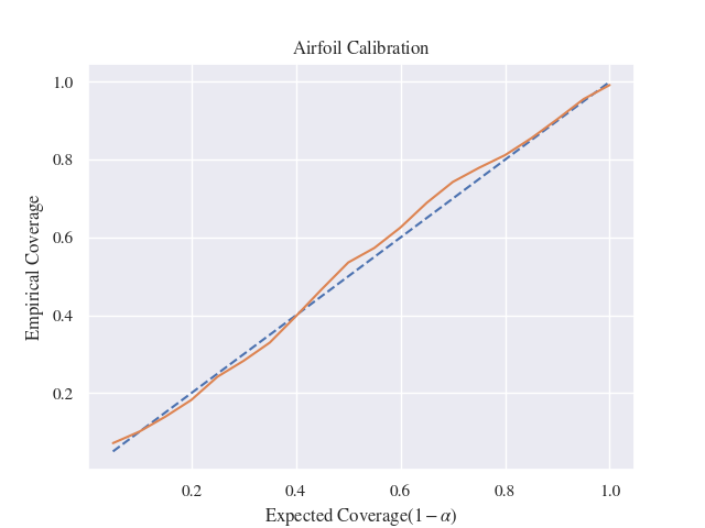
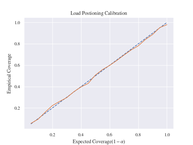
Figure 1: Calibration as assessed over 1,000 i.i.d. test samples. The dashed line is given as reference for what a perfectly calibrated model would look like.

5 Discussion

We have presented CPC, a principled framework for specifying the robust control subproblem in an uncertain control co-design LQR setting. We view such a framework as an important first step in a line of work, suggesting many directions for extension. The most immediate would involve integrating this proposed framework fully into a UCCD pipeline: we focused herein on the robust control subproblem but characterizing the full end-to-end workflow is of great interest. In addition, while we considered the LQR setting herein, many engineering systems in practice involve nonlinear dynamics. In that vein, leveraging insights from Koopman operator theory, where nonlinear dynamical systems can be framed as linear systems under an appropriate change of basis, would be of great interest [58, 59, 60]. A similar nonlinear extension would involve exploring neural operator surrogate models [61]. Further, extending this to the MDP setting would also be of interest; leveraging predict-then-optimize style modeling was undertaken in previous works but has yet to be extended to robust variants thereof [62].

6 Acknowledgements

We acknowledge the support of NSF via grant IIS-2007055.

Appendix A Prediction Region Validity Lemma

Lemma A.1.

Let $f(K,C)$ be a function such that, for any fixed $\theta$, it is non-negative and $L$-Lipschitz in $C\in\mathcal{U}(\theta)$ under the operator norm metric for any $K\in\mathcal{K}(\mathcal{U}(\theta))$, where $\mathcal{K}:\Omega(\Theta)\rightarrow\Omega(\mathcal{C})$ and $\Omega_{1}\subset\Omega_{2}\implies\mathcal{K}(\Omega_{2})\subset\mathcal{K}(\Omega_{1})$. Further assume, for any $C$, that $\max_{K\in\mathcal{K}(C)}f(K,C)<\infty$. Assume further that $\mathcal{P}_{\Theta,C}(C\in\mathcal{U}(\Theta))\geq 1-\alpha$. Then, there is a bounded function $g:\Omega(\Theta)\rightarrow\mathbb{R}$ such that $\Omega_{1}\subset\Omega_{2}\implies g(\Omega_{1})\leq g(\Omega_{2})$ that satisfies:

$$\mathcal{P}_{\Theta,C}\left(0\leq\mathcal{R}(\Theta,C)\leq g(\mathcal{U}(\Theta))\right)\geq 1-\alpha.$$ (12)

Proof.

We consider the event of interest conditionally on a pair $(\theta,C)$ where $\widehat{C}\in\mathcal{U}(\theta)$. By assumption, we then have that $\mathcal{K}(\mathcal{U}(\theta))\subset\mathcal{K}(C)$:

$$\left|\min_{K\in\mathcal{K}(\mathcal{U}(\theta))}\max_{\widehat{C}\in\mathcal{U}(\theta)}f(K,\widehat{C})-\min_{K\in\mathcal{K}(C)}f(K,C)\right|$$

$$\leq\left|\min_{K\in\mathcal{K}(\mathcal{U}(\theta))}\max_{\widehat{C}\in\mathcal{U}(\theta)}f(K,\widehat{C})-\min_{K\in\mathcal{K}(\mathcal{U}(\theta))}f(K,C)\right|+\left|\min_{K\in\mathcal{K}(\mathcal{U}(\theta))}f(K,C)-\min_{K\in\mathcal{K}(C)}f(K,C)\right|$$

We now bound each term separately, starting with the first term:

$$\left|\min_{K\in\mathcal{K}(\mathcal{U}(\theta))}\max_{\widehat{C}\in\mathcal{U}(\theta)}f(K,\widehat{C})-\min_{K\in\mathcal{K}(\mathcal{U}(\theta))}f(K,C)\right|$$

$$\leq\max_{K\in\mathcal{K}(\mathcal{U}(\theta))}|\max_{\widehat{C}\in\mathcal{U}(\theta)}f(K,\widehat{C})-f(K,C)|$$

$$\leq L\max_{\widehat{C}\in\mathcal{U}(\theta)}||\widehat{C}-C||_{2}\leq L\mathrm{diam}(\mathcal{U}(\theta)).$$

The second term can be bounded simply by considering the set difference of $\mathcal{K}(C)$ and $\mathcal{K}(\mathcal{U}(\theta))$ as follows:

$$\left|\min_{K\in\mathcal{K}(\mathcal{U}(\theta))}f(K,C)-\min_{K\in\mathcal{K}(C)}f(K,C)\right|\leq\max_{K\in\mathcal{K}(C)-\mathcal{K}(\mathcal{U}(\theta))}f(K,C)$$

We then define $g(\mathcal{U}(\theta)):=L\mathrm{diam}(\mathcal{U}(\theta))+\max_{K\in\mathcal{K}(C)-\mathcal{K}(\mathcal{U}(\theta))}f(K,C)$. To see $g(\mathcal{U}(\theta))$ is bounded, we consider each term separately. The first follows as $\mathrm{diam}(\mathcal{U}(\theta))<\infty$. For the second, we have that:

$$\max_{K\in\mathcal{K}(C)-\mathcal{K}(\mathcal{U}(\theta))}f(K,C)\leq\max_{K\in\mathcal{K}(C)}f(K,C)<\infty,$$

where the final bound follows by assumption. To observe that $g$ has the desired monotonocity property, we first note that, if $\mathcal{U}_{1}(\theta)\subset\mathcal{U}_{2}(\theta)$, then $\mathrm{diam}(\mathcal{U}_{1}(\theta))\leq\mathrm{diam}(\mathcal{U}_{2}(\theta))$. We similarly have by assumption that, $\mathcal{K}(\mathcal{U}_{2}(\theta))\subset\mathcal{K}(\mathcal{U}_{1}(\theta))$, from which it follows that $\mathcal{K}(C)-\mathcal{K}(\mathcal{U}_{1}(\theta))\subset\mathcal{K}(C)-\mathcal{K}(\mathcal{U}_{2}(\theta))$ and immediately that the maximization problem naturally increases, namely:

$$\max_{K\in\mathcal{K}(\mathcal{U}_{1}(\theta))-\mathcal{K}(C)}f(K,C)\leq\max_{K\in\mathcal{K}(\mathcal{U}_{2}(\theta))-\mathcal{K}(C)}f(K,C).$$

$g$, therefore, satisfies the desired monotonicity property. Since we have the assumption that $\mathcal{P}_{\Theta,C}(C\in\mathcal{U}(\Theta))\geq 1-\alpha$, the result immediately follows. ∎

Appendix B Deterministic Discrete-Time Regret Analysis

Theorem B.1.

Let $J(K,C)$ be the infinite horizon, discrete-time, deterministic analog of that defined in Equation 3, i.e. $J(K,C):=\sum_{t=0}^{\infty}(x_{t}^{\top}(Q+K^{\top}RK)x_{t})$ with $w=0$. Assume that for any fixed $\theta$, $K\in\mathcal{K}(\mathcal{U}(\theta))$, and $C\in\mathcal{U}(\theta)$, $D(K):=\sqrt{n}||Q+K^{\top}RK||_{\infty}||x_{0}||_{\infty}^{2}||W||_{2}<\infty$ and $||CW||<1$. Assume further that $\mathcal{P}_{\Theta,C}(C\in\mathcal{U}(\Theta))\geq 1-\alpha$. Then, there is a function $g:\Omega(\Theta)\rightarrow\mathbb{R}$ such that $\Omega_{1}\subset\Omega_{2}\implies g(\Omega_{1})\leq g(\Omega_{2})$ that satisfies:

$$\mathcal{P}_{\Theta,C}\left(0\leq\mathcal{R}(\Theta,C)\leq g(\mathcal{U}(\Theta))\right)\geq 1-\alpha.$$ (13)

Proof.

We consider any fixed $\theta$ and demonstrate that $J(K,C)$ is non-negative and $L$-Lipschitz in $C\in\mathcal{U}(\theta)$ under the operator norm metric for any $K\in\mathcal{K}(\mathcal{U}(\theta))$, from which Lemma A.1 can be invoked to arrive at the desired conclusion. Given the assumed determinism of the dynamics, we have that $x_{t}=(CW)^{t}x_{0}$, meaning the above objective setup can equivalently be expressed as:

$$\sum_{t=0}^{\infty}x_{0}^{\top}((CW)^{t\top}(Q+K^{\top}RK)(CW)^{t})x_{0},$$ (14)

$J$ is clearly non-negative by construction. To further see that, for any $C$, $\max_{K\in\mathcal{K}(C)}J(K,C)<\infty$, we notice that:

$$\left|\left|\sum_{t=0}^{\infty}x_{0}^{\top}((CW)^{t\top}(Q+K^{\top}RK)(CW)^{t})x_{0}\right|\right|_{2}\leq\sum_{t=0}^{\infty}\left|\left|x_{0}^{\top}((CW)^{t\top}(Q+K^{\top}RK)(CW)^{t})x_{0}\right|\right|_{2}$$

$$\leq\sum_{t=0}^{\infty}||x_{0}||^{2}_{2}||Q+K^{\top}RK||_{2}||CW||^{2t}_{2}=\frac{||x_{0}||^{2}_{2}||Q+K^{\top}RK||_{2}}{1-||CW||^{2}}<\infty,$$

where the finiteness of the final quantity is guaranteed by the assumptions on $D(K)$ and $||CW||<1$.

It, therefore, suffices to demonstrate this objective is Lipschitz continuous with an appropriate Lipschitz constant. Notice the Lipschitz constant can be obtained by bounding the magnitude of the gradient with respect to $C$, which we do as follows

$$\nabla_{C}\left(\sum_{t=0}^{\infty}x_{0}^{\top}((CW)^{t\top}(Q+K^{\top}RK)(CW)^{t})x_{0}\right)$$

$$=\sum_{t=0}^{\infty}t\mathrm{diag}((Q+K^{\top}RK)(CW)^{t}x_{0})(CW)^{(t-1)}\mathrm{diag}(x_{0})W^{\top}$$

$$+\sum_{t=0}^{\infty}t\mathrm{diag}((Q^{\top}+(RK)^{\top}K)(CW)^{t}x_{0})(CW)^{(t-1)}\mathrm{diag}(x_{0})W^{\top}$$

We now bound the magnitude of this quantity as follows:

$$L\leq\max_{C}||\sum_{t=0}^{\infty}t\mathrm{diag}((Q+K^{\top}RK)(CW)^{t}x_{0})(CW)^{(t-1)}\mathrm{diag}(x_{0})W^{\top}$$

$$+\sum_{t=0}^{\infty}t\mathrm{diag}((Q^{\top}+(RK)^{\top}K)(CW)^{t}x_{0})(CW)^{(t-1)}\mathrm{diag}(x_{0})W^{\top}||_{2}$$

$$\leq\max_{C}\sum_{t=0}^{\infty}t\left|\left|\mathrm{diag}((Q+K^{\top}RK)(CW)^{t}x_{0})(CW)^{(t-1)}\mathrm{diag}(x_{0})W^{\top}\right|\right|_{2}$$

$$+\sum_{t=0}^{\infty}t\left|\left|\mathrm{diag}((Q^{\top}+(RK)^{\top}K)(CW)^{t}x_{0})(CW)^{(t-1)}\mathrm{diag}(x_{0})W^{\top}\right|\right|_{2},$$

where we have used $\mathrm{diag}(x_{0})$ for a vector $x_{0}$ to denote a diagonal matrix with $x_{0}$ placed along its main diagonal. We now bound each of these two terms separately, although the structure of the two is the same, so we explicitly show steps for bounding the first, from which the same can be repeated on the second. Importantly, we make use of the fact $||\text{diag}(x_{0})||_{2}=||x_{0}||_{\infty}$ and $||A||_{\infty}\leq\sqrt{n}||A||_{2}$ for $A\in\mathbb{R}^{n\times n}$ as follows:

$$\max_{C}\sum_{t=0}^{\infty}t||\mathrm{diag}((Q+K^{\top}RK)(CW)^{t}x_{0})(CW)^{(t-1)}\mathrm{diag}(x_{0})W^{\top}||_{2}$$

$$\leq\max_{C}\sum_{t=0}^{\infty}t||\mathrm{diag}((Q+K^{\top}RK)(CW)^{t}x_{0})||_{2}||(CW)^{(t-1)}||_{2}||\mathrm{diag}(x_{0})||_{2}||W^{\top}||_{2}$$

$$=\max_{C}\sum_{t=0}^{\infty}t||(Q+K^{\top}RK)(CW)^{t}x_{0}||_{\infty}||x_{0}||_{\infty}||(CW)^{(t-1)}||_{2}||W||_{2}$$

$$\leq\max_{C}\sum_{t=0}^{\infty}t||Q+K^{\top}RK||_{\infty}||(CW)^{t}||_{\infty}||x_{0}||_{\infty}||x_{0}||_{\infty}||(CW)^{(t-1)}||_{2}||W||_{2}$$

$$\leq\max_{C}\sum_{t=0}^{\infty}t(\sqrt{n}||Q+K^{\top}RK||_{\infty}||x_{0}||^{2}_{\infty}||W||_{2})||(CW)^{t}||_{2}||(CW)^{(t-1)}||_{2}.$$

We now collect all terms independent of $t$ into a constant $D(K)=\sqrt{n}||Q+K^{\top}RK||_{\infty}||x_{0}||_{\infty}^{2}||W||_{2}$, leaving us with:

$$\leq\max_{C}D(K)\sum_{t=0}^{\infty}t\left|\left|CW\right|\right|^{2t-1}_{2}=\max_{C}D(K)\frac{\left|\left|CW\right|\right|_{2}}{\left(\left|\left|CW\right|\right|_{2}^{2}-1\right)^{2}}$$

which converges if $\left|\left|CW\right|\right|_{2}<1$, as assumed. ∎

The finite LQR case follows immediately as a corollary of the above, stated below for completeness. Notably, the qualitative nature of the two differs in that no assumptions on the underlying dynamics are necessary in the finite time horizon case, i.e. $||CW||_{2}<1$ is no longer a necessary assumption, as the bound of the suboptimality will necessarily be finite simply by virtue of considering a finite time horizon.

Corollary B.2.

Let $J(K,C)$ be the finite horizon, discrete-time, deterministic analog of that defined in Equation 3, i.e. $J(K,C):=\sum_{t=0}^{T}(x_{t}^{\top}(Q+K^{\top}RK)x_{t})$ with $w=0$. Assume that for any fixed $\theta$, $K\in\mathcal{K}(\mathcal{U}(\theta))$, and $C\in\mathcal{U}(\theta)$, $D(K):=\sqrt{n}||Q+K^{\top}RK||_{\infty}||x_{0}||_{\infty}^{2}||W||_{2}<\infty$. Assume further that $\mathcal{P}_{\Theta,C}(C\in\mathcal{U}(\Theta))\geq 1-\alpha$. Then, there is a function $g:\Omega(\Theta)\rightarrow\mathbb{R}$ such that $\Omega_{1}\subset\Omega_{2}\implies g(\Omega_{1})\leq g(\Omega_{2})$ that satisfies:

$$\mathcal{P}_{\Theta,C}\left(0\leq\mathcal{R}(\Theta,C)\leq g(\mathcal{U}(\Theta))\right)\geq 1-\alpha.$$ (15)

Appendix C Deterministic Continuous-Time Regret Analysis

The proof follows in much the same manner as the discrete-time case, with modest adjustments to the exact specification of the assumptions regarding the dynamics.

Theorem C.1.

Let $J(K,C)$ be the infinite horizon, continuous-time, deterministic analog of that defined in Equation 3, i.e. $J(K,C):=\int_{0}^{\infty}(x(t)^{\top}(Q+K^{\top}RK)x(t))dt$ for $w=0$. Assume that for any fixed $\theta$, $K\in\mathcal{K}(\mathcal{U}(\theta))$, and $C\in\mathcal{U}(\theta)$, $D(K):=\sqrt{n}||Q+K^{\top}RK||_{\infty}||x_{0}||_{\infty}^{2}||W||_{2}<\infty$. Assume further that $\mathcal{P}_{\Theta,C}(C\in\mathcal{U}(\Theta))\geq 1-\alpha$. Then, there is a function $g:\Omega(\Theta)\rightarrow\mathbb{R}$ such that $\Omega_{1}\subset\Omega_{2}\implies g(\Omega_{1})\leq g(\Omega_{2})$ that satisfies:

$$\mathcal{P}_{\Theta,C}\left(0\leq\mathcal{R}(\Theta,C)\leq g(\mathcal{U}(\Theta))\right)\geq 1-\alpha.$$ (16)

Proof.

We consider any fixed $\theta$ and demonstrate the desired properties that $J(K,C)$ is non-negative and $L$-Lipschitz in $C\in\mathcal{U}(\theta)$ under the operator norm metric for any $K\in\mathcal{K}(\mathcal{U}(\theta))$, from which Lemma A.1 can be invoked to arrive at the desired conclusion. Given the assumed determinism of the dynamics, we further have that $x(t)=e^{CWt}x(0)$, meaning the above objective setup can equivalently be expressed with the uncertainty sets related to the objective function, namely as:

$$\int_{0}^{\infty}x(0)^{\top}(e^{CWt})^{\top}(Q+K^{\top}RK)(e^{CWt})x(0)dt.$$ (17)

$J$ is clearly non-negative by construction. To further see that, for any $C$, $\max_{K\in\mathcal{K}(C)}J(K,C)<\infty$, we notice that:

$$\left|\left|\int_{0}^{\infty}(x(0)^{\top}(e^{CWt})^{\top}(Q+K^{\top}RK)(e^{CWt})x(0))dt\right|\right|_{2}$$

$$\leq\int_{0}^{\infty}\left|\left|x(0)^{\top}(e^{CWt})^{\top}(Q+K^{\top}RK)(e^{CWt})x(0)\right|\right|_{2}dt$$

$$\leq\int_{0}^{\infty}||x(0)||^{2}_{2}||e^{CWt}||^{2}_{2}||Q+K^{\top}RK||^{2}_{2}dt=||x(0)||^{2}_{2}||Q+K^{\top}RK||^{2}_{2}\int_{0}^{\infty}||e^{CWt}||^{2}_{2}dt$$

$$\leq||x(0)||^{2}_{2}||Q+K^{\top}RK||^{2}_{2}\int_{0}^{\infty}\beta(C)^{2}e^{-2\alpha(C)t}dt=\frac{\beta(C)^{2}||x(0)||^{2}_{2}||Q+K^{\top}RK||^{2}_{2}}{2\alpha(C)}<\infty$$

where we used the fact for any $K\in\mathcal{K}(C)$, we have that $CW$ is Hurwitz by definition, which exhibits the standard matrix exponential bound $||e^{CWt}||\leq\beta(C)e^{-\alpha(C)t}$ for some $\alpha(C),\beta(C)>0$.

It, therefore, suffices to demonstrate this objective is Lipschitz continuous with an appropriate Lipschitz constant. We again proceed by bounding the norm of the gradient as follows:

$$\nabla_{C}\left(\int_{0}^{\infty}x(0)^{\top}(e^{CWt})^{\top}(Q+K^{\top}RK)(e^{CWt})x(0)dt\right)$$

$$=\int_{0}^{\infty}t\mathrm{diag}((Q+K^{\top}RK)e^{CWt}x(0))e^{CWt}\mathrm{diag}(x(0))W^{\top}dt$$

$$+\int_{0}^{\infty}t\mathrm{diag}((Q^{\top}+(RK)^{\top}K)e^{CWt}x(0))e^{CWt}\mathrm{diag}(x(0))W^{\top}dt$$

We again bound each of these two terms separately, as follows:

$$\max_{C}\left|\left|\int_{0}^{\infty}t\mathrm{diag}((Q+K^{\top}RK)e^{CWt}x(0))e^{CWt}\mathrm{diag}(x(0))W^{\top}dt\right|\right|_{2}$$

$$\leq\max_{C}\int_{0}^{\infty}t\left|\left|\mathrm{diag}((Q+K^{\top}RK)e^{CWt}x(0))\right|\right|_{2}\left|\left|e^{CWt}\right|\right|_{2}\left|\left|\mathrm{diag}(x(0))\right|\right|_{2}\left|\left|W^{\top}\right|\right|_{2}dt$$

$$=\max_{C}\int_{0}^{\infty}t\left|\left|(Q+K^{\top}RK)e^{CWt}x(0)\right|\right|_{\infty}\left|\left|e^{CWt}\right|\right|_{2}\left|\left|x(0)\right|\right|_{\infty}\left|\left|W\right|\right|_{2}dt$$

$$\leq\max_{C}\int_{0}^{\infty}t(\sqrt{n}\left|\left|Q+K^{\top}RK\right|\right|_{\infty}\left|\left|W\right|\right|_{2}\left|\left|x(0)\right|\right|^{2}_{\infty})\left|\left|e^{CWt}\right|\right|^{2}_{2}dt.$$

Collecting all terms independent of $t$ into a constant $D(K)=\sqrt{n}||Q+K^{\top}RK||_{\infty}||W||_{2}||x(0)||^{2}_{\infty}$ and using the bound $||e^{CWt}||\leq\beta(C)e^{-\alpha(C)t}$, we reach the conclusion as:

$$=\max_{C}D(K)\int_{0}^{\infty}t\left|\left|e^{CWt}\right|\right|^{2}_{2}dt\leq D(K)\beta(C)^{2}\int_{0}^{\infty}te^{-2\alpha(C)t}dt=\max_{C}\frac{D(K)\beta(C)^{2}}{4\alpha(C)^{2}},$$

as desired. ∎

Once again, the proof in the finite time horizon case follows equivalently.

Corollary C.2.

Let $J(K,C)$ be the finite horizon, continuous-time, deterministic analog of that defined in Equation 3, i.e. $J(K,C):=\int_{0}^{T}(x(t)^{\top}(Q+K^{\top}RK)x(t))dt$ for $w=0$. Assume that for any fixed $\theta$, $K\in\mathcal{K}(\mathcal{U}(\theta))$, and $C\in\mathcal{U}(\theta)$, $D(K):=\sqrt{n}||Q+K^{\top}RK||_{\infty}||x_{0}||_{\infty}^{2}||W||_{2}<\infty$. Assume further that $\mathcal{P}_{\Theta,C}(C\in\mathcal{U}(\Theta))\geq 1-\alpha$. Then, there is a function $g:\Omega(\Theta)\rightarrow\mathbb{R}$ such that $\Omega_{1}\subset\Omega_{2}\implies g(\Omega_{1})\leq g(\Omega_{2})$ that satisfies:

$$\mathcal{P}_{\Theta,C}\left(0\leq\mathcal{R}(\Theta,C)\leq g(\mathcal{U}(\Theta))\right)\geq 1-\alpha.$$ (18)

Appendix D Stochastic Discrete-Time Regret Analysis

Theorem D.1.

Let $J(K,C)$ be the infinite horizon, discrete-time, stochastic analog of that defined in Equation 3, i.e. $J(K,C):=\sum_{t=0}^{\infty}(x_{t}^{\top}(Q+K^{\top}RK)x_{t})$ with $w_{t}\sim\mathcal{N}(0,\Sigma)$ i.i.d. across $t$. Assume that for any fixed $\theta$, $K\in\mathcal{K}(\mathcal{U}(\theta))$, and $C\in\mathcal{U}(\theta)$: (1) $||Q_{t}+K^{\top}R_{t}K||\leq\beta_{1}e^{-\alpha_{1}t}$ for some constants $\alpha_{1},\beta_{1}>0$ such that $\min_{C}(2\alpha_{2}(C)+\alpha_{1})>0$ for $\alpha_{2}(C):=\min_{K\in\mathcal{K}(C)}(-\log(||CW||))$ and (2) $D_{1}(K):=\max_{t}\sqrt{n}||Q(t)+K^{\top}R(t)K||_{\infty}||x_{0}||_{\infty}^{2}||W||_{2}<\infty$, $D_{2}(K):=||\Sigma||_{2}||W||_{2}<\infty$, and $||CW||<1$. Assume further that $\mathcal{P}_{\Theta,C}(C\in\mathcal{U}(\Theta))\geq 1-\alpha$. Then, there is a function $g:\Omega(\Theta)\rightarrow\mathbb{R}$ such that $\Omega_{1}\subset\Omega_{2}\implies g(\Omega_{1})\leq g(\Omega_{2})$ that satisfies:

$$\mathcal{P}_{\Theta,C}\left(0\leq\mathcal{R}(\Theta,C)\leq g(\mathcal{U}(\Theta))\right)\geq 1-\alpha.$$ (19)

Proof.

We again consider any fixed $\theta$ and demonstrate the desired properties that $J(K,C)$ is non-negative and $L$-Lipschitz in $C\in\mathcal{U}(\theta)$ under the operator norm metric for any $K\in\mathcal{K}(\mathcal{U}(\theta))$, from which Lemma A.1 can be invoked to arrive at the desired conclusion. Notice the objective can be reformulated in the standard manner as follows:

$$J(K,C):=\mathbb{E}[\sum_{t=0}^{\infty}(x_{t}^{\top}(Q_{t}+K^{\top}R_{t}K)x_{t})]=\sum_{t=0}^{\infty}\mathbb{E}[(x_{t}^{\top}(Q_{t}+K^{\top}R_{t}K)x_{t})]$$

$$=\sum_{t=0}^{\infty}\mathbb{E}[\mathrm{Tr}(x_{t}^{\top}(Q_{t}+K^{\top}R_{t}K)x_{t})]=\sum_{t=0}^{\infty}\mathbb{E}[\mathrm{Tr}((Q_{t}+K^{\top}R_{t}K)x_{t}x_{t}^{\top})]]$$

$$=\sum_{t=0}^{\infty}\mathrm{Tr}((Q_{t}+K^{\top}R_{t}K)\mathbb{E}[x_{t}x_{t}^{\top}])=\sum_{t=0}^{\infty}\mathrm{Tr}((Q_{t}+K^{\top}R_{t}K)(\mathbb{E}[x_{t}]\mathbb{E}[x_{t}]^{\top}+\mathrm{Var}(x_{t}))).$$

We now use the following computations to evaluate this final expression:

$$\mathbb{E}[x_{t}]=\mathbb{E}[(CW)x_{t-1}+w_{t}]$$

$$=\mathbb{E}[(CW)x_{t-1}]+\mathbb{E}[w_{t}]=\mathbb{E}[(CW)((CW)x_{t-2}+w_{t-1})]$$

$$=\mathbb{E}[(CW)^{2}x_{t-2}]+(CW)\mathbb{E}[w_{t-1})]=...=(CW)^{t}x_{0}.$$

$$\mathrm{Var}(x_{t})=\mathrm{Var}((CW)x_{t-1}+w_{t})=(CW)\mathrm{Var}(x_{t-1})(CW)^{\top}+\Sigma$$

$$=(CW)\mathrm{Var}(x_{t-2})(CW)^{\top}+(CW)\Sigma(CW)^{\top}+\Sigma=...=\sum_{k=0}^{t-1}(CW)^{k}\Sigma(CW)^{k\top}.$$

With these simplifications, we are left with:

$$J(K,C)=\sum_{t=0}^{\infty}x_{0}^{\top}(CW)^{t\top}(Q_{t}+K^{\top}R_{t}K)(CW)^{t}x_{0}$$

$$+\sum_{t=0}^{\infty}\sum_{k=0}^{t-1}\mathrm{Tr}((Q_{t}+K^{\top}R_{t}K)(CW)^{k}\Sigma(CW)^{k\top}))$$

$J$ is clearly non-negative by construction. To further see that, for any $C$, $\max_{K\in\mathcal{K}(C)}J(K,C)<\infty$, we first note that the first term was bounded in the proof of Theorem B.1, where the assumptions on $D_{1}(K)$ and $||CW||$ permit its invocation. For the second term, we proceed similarly, as follows:

$$\leq\sum_{t=0}^{\infty}\sum_{k=0}^{t-1}\left|\left|\mathrm{Tr}((Q_{t}+K^{\top}R_{t}K)(CW)^{k}\Sigma(CW)^{k\top}))\right|\right|_{2}$$

$$\leq||\Sigma||_{2}\sum_{t=0}^{\infty}||Q_{t}+K^{\top}R_{t}K||_{2}\sum_{k=0}^{t-1}||CW||^{2k}_{2}\leq||\Sigma||_{2}\int_{0}^{\infty}||Q_{t}+K^{\top}R_{t}K||_{2}\int_{0}^{t}||CW||^{2k}_{2}dkdt$$

$$\leq\frac{||\Sigma||_{2}}{2\log(||CW||_{2})}\int_{0}^{\infty}||Q_{t}+K^{\top}R_{t}K||_{2}(||CW||_{2}^{2t}-1)dt$$

$$\leq\beta_{1}\frac{||\Sigma||_{2}}{2\log(||CW||_{2})}\int_{0}^{\infty}e^{-\alpha_{1}t}(||CW||_{2}^{2t}-1)dt<\infty$$

where we used the assumption that $||CW||_{2}<1$ to ensure convergence of the integral.

We demonstrate this quantity is Lipschitz continuous with an appropriate Lipschitz constant, again by bounding the gradient. The bound for the first term was demonstrated in the proof of Theorem B.1, for which reason we solely present that of the second term as follows:

$$\sum_{t=0}^{\infty}\sum_{k=0}^{t-1}\nabla_{C}\mathrm{Tr}((Q_{t}+K^{\top}R_{t}K)(CW)^{k}\Sigma(CW)^{k\top}))$$

$$=\sum_{t=0}^{\infty}\sum_{k=0}^{t-1}k((((Q_{t}+K^{\top}R_{t}K)^{\top}(CW)^{k}\Sigma^{\top})\odot(CW)^{(k-1)})W^{\top}+$$

$$\sum_{t=0}^{\infty}\sum_{k=0}^{t-1}k(((Q_{t}+K^{\top}R_{t}K)(CW)^{k}\Sigma)\odot(CW)^{(k-1)})W^{\top}$$

We now bound each of these two terms separately, although the structure of the two is the same, so we explicitly show steps for bounding the first, from which the same can be repeated on the second.

$$\max_{C}||\sum_{t=0}^{\infty}\sum_{k=0}^{t-1}k((((Q_{t}+K^{\top}R_{t}K)^{\top}(CW)^{k}\Sigma^{\top})\odot(CW)^{(k-1)})W^{\top}||_{2}$$

$$\leq\max_{C}\sum_{t=0}^{\infty}\sum_{k=0}^{t-1}k||((Q_{t}+K^{\top}R_{t}K)^{\top}(CW)^{k}\Sigma^{\top})\odot(CW)^{(k-1)}||_{2}||W||_{2}$$

$$\leq\max_{C}\sum_{t=0}^{\infty}\sum_{k=0}^{t-1}k||Q_{t}+K^{\top}R_{t}K||_{2}||(CW)^{k}||_{2}||\Sigma||_{2}||(CW)^{(k-1)}||_{2}||W||_{2}$$

$$\leq\max_{C}\sum_{t=0}^{\infty}\sum_{k=0}^{t-1}k||Q_{t}+K^{\top}R_{t}K||_{2}||\Sigma||_{2}||W||_{2}||CW||^{(2k-1)}_{2}$$

We again now collect all terms independent of $t$ into a constant $D_{2}(K)=||\Sigma||_{2}||W||_{2}$. We prove the convergence by first expressing $\alpha_{2}(C)\leq-\log(||CW||)\implies||CW||\leq e^{-\alpha_{2}(C)}$, giving us

$$\leq\max_{C}D_{2}(K)\beta_{1}\int_{0}^{\infty}e^{-\alpha_{1}t}\int_{0}^{t}ke^{-2\alpha_{2}(C)k}dkdt$$

$$\leq\max_{C}\frac{D_{2}(K)\beta_{1}}{4\alpha_{2}(C)^{2}}\int_{0}^{\infty}e^{-\alpha_{1}t}\left(e^{-2\alpha_{2}(C)t}(-2\alpha_{2}(C)t+e^{2\alpha_{2}(C)t}-1)\right)dt$$

$$=\max_{C}\frac{D_{2}(K)\beta_{1}}{\alpha_{1}(2\alpha_{2}(C)+\alpha_{1})^{2}},$$

where the final convergence is guaranteed if $\min_{C}(2\alpha_{2}(C)+\alpha_{1})>0$ as desired. ∎

Appendix E Stochastic Continuous-Time Regret Analysis

Theorem E.1.

Let $J(K,C)$ be the infinite horizon, continuous-time, stochastic analog of that defined in Equation 3, i.e. $J(K,C):=\mathbb{E}\left[\int_{0}^{\infty}(x(t)^{\top}(Q(t)+K^{\top}R(t)K)x(t))dt\right]$ with $w(t)$ a white noise process with spectral density $\Sigma$. Assume that for any fixed $\theta$, $K\in\mathcal{K}(\mathcal{U}(\theta))$, and $C\in\mathcal{U}(\theta)$: (1) there exist constants $\alpha_{1},\beta_{1}>0$ such that $||Q(t)+K^{\top}R(t)K||\leq\beta_{1}e^{-\alpha_{1}t}$ and $\min_{C}(2\alpha_{2}(C)+\alpha_{1})>0$ where $\alpha_{2}(C):=\max_{K\in\mathcal{K}(C)}(-\max_{i}\mathrm{Re}(\lambda_{i}(CW)))$ and (2) $D_{1}(K):=\max_{t}\sqrt{n}||Q(t)+K^{\top}R(t)K||_{\infty}||x_{0}||_{\infty}^{2}||W||_{2}<\infty$ and $D_{2}(K):=||\Sigma||_{2}||W||_{2}<\infty$. Assume further that $\mathcal{P}_{\Theta,C}(C\in\mathcal{U}(\Theta))\geq 1-\alpha$. Then, there is a function $g:\Omega(\Theta)\rightarrow\mathbb{R}$ such that $\Omega_{1}\subset\Omega_{2}\implies g(\Omega_{1})\leq g(\Omega_{2})$ that satisfies:

$$\mathcal{P}_{\Theta,C}\left(0\leq\mathcal{R}(\Theta,C)\leq g(\mathcal{U}(\Theta))\right)\geq 1-\alpha.$$ (20)

Proof.

We again consider any fixed $\theta$ and demonstrate the desired properties that $J(K,C)$ is non-negative and $L$-Lipschitz in $C\in\mathcal{U}(\theta)$ under the operator norm metric for any $K\in\mathcal{K}(\mathcal{U}(\theta))$, from which Lemma A.1 can be invoked to arrive at the desired conclusion. Notice the objective can be reformulated in the standard manner as follows:

$$J(K,C):=\mathbb{E}\left[\int_{0}^{\infty}(x(t)^{\top}(Q(t)+K^{\top}R(t)K)x(t))dt\right]$$

$$=\int_{0}^{\infty}\mathbb{E}[(x(t)^{\top}(Q(t)+K^{\top}R(t)K)x(t))]dt=\int_{0}^{\infty}\mathbb{E}[\mathrm{Tr}(x(t)^{\top}(Q(t)+K^{\top}R(t)K)x(t))]dt$$

$$=\int_{0}^{\infty}\mathbb{E}[\mathrm{Tr}((Q(t)+K^{\top}R(t)K)x(t)x(t)^{\top})]]dt=\int_{0}^{\infty}\mathrm{Tr}((Q(t)+K^{\top}R(t)K)\mathbb{E}[x(t)x(t)^{\top}])dt$$

$$=\int_{0}^{\infty}\mathrm{Tr}((Q(t)+K^{\top}R(t)K)(\mathbb{E}[x(t)]\mathbb{E}[x(t)]^{\top}+\mathrm{Var}(x(t))))dt.$$

We now obtain the expressions for $\mathbb{E}[x(t)]$ and $\mathrm{Var}(x(t))$ using standard results from stochastic differential equations. For a full review on this topic, see [63]:

$$J(K,C)=\int_{0}^{\infty}x(0)^{\top}(e^{CWt})^{\top}(Q(t)+K^{\top}R(t)K)(e^{CWt})x(0)dt$$

$$+\int_{0}^{\infty}\int_{0}^{t}\mathrm{Tr}((Q(t)+K^{\top}R(t)K)e^{CWk}\Sigma e^{CWk\top})dkdt$$

$J$ is clearly non-negative by construction. To further see that, for any $C$, $\max_{K\in\mathcal{K}(C)}J(K,C)<\infty$, we first note that the first term was bounded in the proof of Theorem C.1. For the second term, we proceed similarly, as follows:

$$\left|\left|\int_{0}^{\infty}\int_{0}^{t}\mathrm{Tr}((Q(t)+K^{\top}R(t)K)e^{CWk}\Sigma e^{CWk\top})dkdt\right|\right|_{2}$$

$$\leq\int_{0}^{\infty}\int_{0}^{t}\left|\left|\mathrm{Tr}((Q(t)+K^{\top}R(t)K)e^{CWk}\Sigma e^{CWk\top})\right|\right|_{2}dkdt$$

$$\leq\int_{0}^{\infty}\int_{0}^{t}||\Sigma||_{2}||Q(t)+K^{\top}R(t)K||_{2}||e^{CWk}||^{2}_{2}dkdt$$

$$\leq||\Sigma||_{2}\int_{0}^{\infty}\beta_{1}e^{-\alpha_{1}t}\int_{0}^{t}\beta_{2}(C)^{2}e^{-2\alpha_{2}(C)k}dkdt$$

$$=||\Sigma||_{2}\frac{\beta_{1}\beta_{2}(C)^{2}}{2\alpha_{2}(C)}\int_{0}^{\infty}e^{-\alpha_{1}t}\left(1-e^{-2\alpha_{2}(C)t}\right)dt=||\Sigma||_{2}\frac{\beta_{1}\beta_{2}(C)^{2}}{2\alpha_{2}(C)}\left(\frac{1}{\alpha_{1}}-\frac{1}{\alpha_{1}+2\alpha_{2}(C)}\right)$$

$$=||\Sigma||_{2}\frac{\beta_{1}\beta_{2}(C)^{2}}{\alpha_{1}(\alpha_{1}+2\alpha_{2}(C))}<\infty$$

where we used the assumption that $\min_{C}(\alpha_{1}+2\alpha_{2}(C))>0$ to ensure convergence and fact that for any $K\in\mathcal{K}(C)$, $CW$ is Hurwitz by definition, which exhibits the well-known matrix exponential bound $||e^{CWt}||\leq\beta_{2}(C)e^{-\alpha_{2}(C)t}$.

We demonstrate this quantity is Lipschitz continuous with an appropriate Lipschitz constant, again by bounding the gradient in much the same manner as the above bound. The bound for the first term was demonstrated in the proof of Theorem B.1, which holds under the finiteness assumption of $D_{1}(K)$. We, thus, solely present that of the second term as follows:

$$\int_{0}^{\infty}\int_{0}^{t}\nabla_{C}\mathrm{Tr}((Q(t)+K^{\top}R(t)K)e^{(CW)k}\Sigma e^{(CW)k\top})dkdt$$

$$=\int_{0}^{\infty}\int_{0}^{t}k(((Q(t)^{\top}+(R(t)K)^{\top}K)e^{kCW}\Sigma^{\top})\odot e^{kCW})W^{\top}dkdt$$

$$+\int_{0}^{\infty}\int_{0}^{t}k(((Q(t)+K^{\top}R(t)K)e^{kCW}\Sigma)\odot e^{kCW})W^{\top}$$

We now bound each of these two terms separately, although the structure of the two is the same, so we explicitly show steps for bounding the first, from which the same can be repeated on the second.

$$L\leq\max_{C}||\int_{0}^{\infty}\int_{0}^{t}k(((Q(t)^{\top}+(R(t)K)^{\top}K)e^{kCW}\Sigma^{\top})\odot e^{kCW})W^{\top}dkdt||_{2}$$

$$\leq\max_{C}\int_{0}^{\infty}\int_{0}^{t}k||Q(t)+K^{\top}R(t)K||_{2}||\Sigma||_{2}||W||_{2}||e^{kCW}||^{2}_{2}dkdt$$

We again now collect all terms independent of $t$ into a constant $D_{2}(K)=||\Sigma||_{2}||W||_{2}$, leaving

$$\leq\max_{C}D_{2}(K)\int_{0}^{\infty}\beta_{1}e^{-\alpha_{1}t}\int_{0}^{t}k\beta_{2}(C)^{2}e^{-2\alpha_{2}(C)k}dkdt$$

$$=\max_{C}\frac{D_{2}(K)\beta_{1}\beta_{2}(C)^{2}}{4\alpha_{2}^{2}(C)}\int_{0}^{\infty}e^{-\alpha_{1}t}\left(1-2\alpha_{2}(C)te^{-2\alpha_{2}(C)t}-e^{-2\alpha_{2}(C)t}\right)dt$$

$$=\max_{C}\frac{D_{2}(K)\beta_{1}\beta_{2}(C)^{2}}{4\alpha_{2}^{2}(C)}\left(\frac{1}{\alpha_{1}}-\frac{2\alpha_{2}(C)}{(\alpha_{1}+2\alpha_{2}(C))^{2}}-\frac{1}{\alpha_{1}+2\alpha_{2}(C)}\right)=\max_{C}\frac{D_{2}(K)\beta_{1}\beta_{2}(C)^{2}}{\alpha_{1}(\alpha_{1}+2\alpha_{2}(C))^{2}}$$

We, therefore, again have the desired upper bound on the Lipschitz constant, as desired. ∎

Appendix F Coverage Guarantees Under Noisy Observations

Theorem F.1.

Let $\widetilde{C}=C+\epsilon$ where $\text{vec}(\epsilon)\sim\mathcal{N}(0,\Sigma)$. Assume $\mathcal{U}(\theta)=\{C^{\prime}\mid||f(\theta)-C^{\prime}||_{2}\leq\widehat{q}\}$ satisfies $\mathcal{P}_{\Theta,\widetilde{C}}(\widetilde{C}\in\mathcal{U}(\Theta))\geq 1-\alpha$. If for any $\theta\in\Theta$ and $\delta>0$, $\mathcal{P}_{C\mid\Theta=\theta}(\widehat{q}^{2}-\delta\leq\|C-f(\theta)\|_{2}^{2}\leq\widehat{q}^{2})>\mathcal{P}_{C\mid\Theta=\theta}(\widehat{q}^{2}\leq\|C-f(\theta)\|_{2}^{2}\leq\widehat{q}^{2}+\delta)$, then

$$\mathcal{P}_{\Theta,C}(C\in\mathcal{U}(\Theta))\geq\mathcal{P}_{\Theta,\widetilde{C}}(\widetilde{C}\in\mathcal{U}(\Theta))\geq 1-\alpha.$$

Proof.

Given our assumption that $\mathcal{P}_{\Theta,\widetilde{C}}(\widetilde{C}\in\mathcal{U}(\Theta))\geq 1-\alpha$, it suffices to show that $\mathcal{P}_{C|\Theta=\theta}(C\in\mathcal{U}(\theta))\geq\mathcal{P}_{\widetilde{C}\mid\Theta=\theta}(\widetilde{C}\in\mathcal{U}(\theta))$ for all $\theta$, as the conclusion can be drawn by the law of total probability:

$$\mathcal{P}_{\widetilde{C}\mid\Theta=\theta}(\widetilde{C}\in\mathcal{U}(\theta))$$

$$=\mathcal{P}_{\widetilde{C}\mid\Theta=\theta}\left(\left\|\widetilde{C}-f(\theta)\right\|_{2}^{2}\leq\widehat{q}^{2}\right)$$

$$=\mathcal{P}_{C,\epsilon\mid\Theta=\theta}\left(\underset{\|x\|=1}{\sup}\left\{\left\|Cx+\epsilon x-f(\theta)x\right\|_{2}^{2}\right\}\leq\widehat{q}^{2}\right)$$

$$=\mathcal{P}_{C,\epsilon\mid\Theta=\theta}\left(\underset{\|x\|=1}{\sup}\left\{\left\|Cx-f(\theta)x\right\|_{2}^{2}+2x^{T}\epsilon^{T}\left(Cx-f(\theta)x\right)+\|\epsilon x\|_{2}^{2}\right\}\leq\widehat{q}^{2}\right)$$

$$\leq\mathcal{P}_{C,\epsilon\mid\Theta=\theta}\left(\underset{\|x\|=1}{\sup}\left\{\left\|Cx-f(\theta)x\right\|_{2}^{2}\right\}+2x^{*^{T}}\epsilon^{T}\left(Cx^{*}-f(\theta)x^{*}\right)\leq\widehat{q}^{2}\right)$$

$$\text{where}\left\|Cx^{*}-f(\theta)x^{*}\right\|_{2}^{2}=\underset{\|x\|=1}{\sup}\left\{\left\|Cx-f(\theta)x\right\|_{2}^{2}\right\}$$

Let $\delta=2x^{*^{T}}\epsilon^{T}\left(Cx^{*}-f(\theta)x^{*}\right)$. Then:

$$:=\mathcal{P}_{C,\delta\mid\Theta=\theta}\left(\left\|C-f(\theta)\right\|_{2}^{2}+\delta\leq\widehat{q}^{2}\right)$$

$$=\mathcal{P}_{C\mid\Theta=\theta,\delta>0}\left(\left\|C-f(\theta)\right\|_{2}^{2}+\delta\leq\widehat{q}^{2}\right)\mathcal{P}_{C\mid\Theta=\theta}(\delta>0)$$

$$\quad+\mathcal{P}_{C\mid\Theta=\theta,\delta\leq 0}\left(\left\|C-f(\theta)\right\|_{2}^{2}+\delta\leq\widehat{q}^{2}\right)\mathcal{P}_{C\mid\Theta=\theta}(\delta\leq 0)$$

$$=\mathcal{P}_{C\mid\Theta=\theta,\delta>0}\left(\left\|C-f(\theta)\right\|_{2}^{2}\leq\widehat{q}^{2}-\delta\right)\mathcal{P}_{C\mid\Theta=\theta}(\delta>0)$$

$$\quad+\mathcal{P}_{C\mid\Theta=\theta,\delta>0}\left(\left\|C-f(\theta)\right\|_{2}^{2}\leq\widehat{q}^{2}+\delta\right)\mathcal{P}_{C\mid\Theta=\theta}(\delta\leq 0).$$

$$=\mathcal{P}_{C\mid\Theta=\theta}\left(\left\|C-f(\theta)\right\|_{2}^{2}\leq\widehat{q}^{2}\right)$$

$$\quad-\mathcal{P}_{C\mid\Theta=\theta}\left(\delta>0\right)\mathcal{P}_{C\mid\Theta=\theta,\delta>0}\left(\left\|C-f(\theta)\right\|_{2}^{2}\leq\widehat{q}^{2}\right)$$

$$\quad-\mathcal{P}_{C\mid\Theta=\theta}\left(\delta\leq 0\right)\mathcal{P}_{C\mid\Theta=\theta,\delta\leq 0}\left(\left\|C-f(\theta)\right\|_{2}^{2}\leq\widehat{q}^{2}\right)$$

$$\quad+\mathcal{P}_{C\mid\Theta=\theta}\left(\delta>0\right)\mathbb{E}_{\delta>0}\left[\mathcal{P}_{C\mid\Theta=\theta}\left(\left\|C-f(\theta)\right\|_{2}^{2}\leq\widehat{q}^{2}-\delta\right)\right]$$

$$\quad+\mathcal{P}_{C\mid\Theta=\theta}\left(\delta\leq 0\right)\mathbb{E}_{\delta>0}\left[\mathcal{P}_{C,\delta\mid\Theta=\theta}\left(\left\|C-f(\theta)\right\|_{2}^{2}\leq\widehat{q}^{2}+\delta\right)\right]$$

$$=\mathcal{P}_{C\mid\Theta=\theta}\left(\left\|C-f(\theta)\right\|_{2}^{2}\leq\widehat{q}^{2}\right)$$

$$\quad-\mathcal{P}_{C\mid\Theta=\theta}\left(\delta>0\right)\mathbb{E}_{\delta>0}\left[\mathcal{P}_{C\mid\Theta=\theta}\left(\left\|C-f(\theta)\right\|_{2}^{2}\leq\widehat{q}^{2}\right)-\mathcal{P}_{C\mid\Theta=\theta}\left(\left\|C-f(\theta)\right\|_{2}^{2}\leq\widehat{q}^{2}-\delta\right)\right]$$

$$\quad+\mathcal{P}_{C\mid\Theta=\theta}\left(\delta\leq 0\right)\mathbb{E}_{\delta>0}\left[\mathcal{P}_{C\mid\Theta=\theta}\left(\left\|C-f(\theta)\right\|_{2}^{2}\leq\widehat{q}^{2}+\delta\right)-\mathcal{P}_{C\mid\Theta=\theta}\left(\left\|C-f(\theta)\right\|_{2}^{2}\leq\widehat{q}^{2}\right)\right]$$

$$=\mathcal{P}_{C\mid\Theta=\theta}\left(\left\|C-f(\theta)\right\|_{2}^{2}\leq\widehat{q}^{2}\right)$$

$$\quad-\mathcal{P}_{C\mid\Theta=\theta}\left(\delta>0\right)\mathbb{E}_{\delta>0}\left[\mathcal{P}_{C\mid\Theta=\theta}\left(\widehat{q}^{2}-\delta\leq\left\|C-f(\theta)\right\|_{2}^{2}\leq\widehat{q}^{2}\right)\right]$$

$$\quad+\mathcal{P}_{C\mid\Theta=\theta}\left(\delta\leq 0\right)\mathbb{E}_{\delta>0}\left[\mathcal{P}_{C\mid\Theta=\theta}\left(\widehat{q}^{2}\leq\left\|C-f(\theta)\right\|_{2}^{2}\leq\widehat{q}^{2}+\delta\right)\right].$$

We, therefore, have that $\mathcal{P}_{\widetilde{C}\mid\Theta=\theta}(\widetilde{C}\in\mathcal{U}(\theta))\leq\mathcal{P}_{C\mid\Theta=\theta}\left(\left\|C-f(\theta)\right\|_{2}^{2}\leq\widehat{q}^{2}\right)+\Delta$, where

$$\Delta :=\mathcal{P}_{C\mid\Theta=\theta}\left(\delta\leq 0\right)\mathbb{E}_{\delta>0}\left[\mathcal{P}_{C\mid\Theta=\theta}\left(\widehat{q}^{2}\leq\left\|C-f(\theta)\right\|_{2}^{2}\leq\widehat{q}^{2}+\delta\right)\right]$$

$$-\mathcal{P}_{C\mid\Theta=\theta}\left(\delta>0\right)\mathbb{E}_{\delta>0}\left[\mathcal{P}_{C\mid\Theta=\theta}\left(\widehat{q}^{2}-\delta\leq\left\|C-f(\theta)\right\|_{2}^{2}\leq\widehat{q}^{2}\right)\right]$$

By the assumption, we know that for all $\delta>0$:

$$\mathcal{P}_{C\mid\Theta=\theta}\left(\widehat{q}^{2}-\delta\leq\left\|C-f(\theta)\right\|_{2}^{2}\leq\widehat{q}^{2}\right)>\mathcal{P}_{C\mid\Theta=\theta}\left(\widehat{q}^{2}\leq\left\|C-f(\theta)\right\|_{2}^{2}\leq\widehat{q}^{2}+\delta\right).$$

We also know that $\mathcal{P}_{C\mid\Theta=\theta}(\delta\leq 0)\leq\mathcal{P}_{C\mid\Theta=\theta}(\delta\geq 0)$ since

$$\mathcal{P}_{C,\epsilon\mid\Theta=\theta}(\delta\leq 0) =\mathcal{P}_{C,\epsilon\mid\Theta=\theta}\left(2x^{*^{T}}\epsilon^{T}\left(Cx^{*}-f(\theta)x^{*}\right)\leq 0\right)$$

$$=\mathbb{E}_{C\mid\Theta=\theta}\left[\mathcal{P}_{\epsilon\mid C=c,\Theta=\theta}\left(x^{*^{T}}\epsilon^{T}\left(c-f(\theta)\right)x^{*}\leq 0\right)\right]$$

$$=\mathbb{E}_{C\mid\Theta=\theta}\left[0.5\right]$$

$$=0.5$$

Therefore, $\mathcal{P}_{\widetilde{C}\mid\Theta=\theta}\left(\left\|\widetilde{C}-f(\theta)\right\|_{2}\leq\widehat{q}\right)-\mathcal{P}_{C\mid\Theta=\theta}\left(\left\|C-f(\theta)\right\|_{2}\leq\widehat{q}\right)\leq\Delta\leq 0$ ∎

Appendix G LQR $C$ Gradient

We follow the presentation of [54] to provide the derivation of $\nabla_{C}J(K,C)$. Note that the following derivation is given for the discrete-time setting; the continuous-time derivation follows in a similar fashion with a modification in the Lyapunov equations.

Lemma G.1.

Let $J(K,C)$ be the infinite horizon, discrete-time, deterministic analog of that defined in Equation 3, i.e. $J(K,C):=\sum_{t=0}^{\infty}(x_{t}^{\top}(Q+K^{\top}RK)x_{t})$ for $w=0$. Then,

$$\nabla_{C}J(K,C)=2P_{K}CWX_{K}W^{T},$$ (21)

where $X_{K}$ and $P_{K}$ respectively solve the following two Lyapunov equations: $\Delta_{K}X_{K}\Delta^{\top}_{K}-X_{K}=0$ and $P_{K}=\Delta^{\top}_{K}P_{K}\Delta_{K}+Q+K^{\top}RK$, where $\Delta_{K}:=A-BK$.

Proof.

By the standard reformulation of $J(K,C)$ as described in [54], we can rewrite $J(K,C,x_{0})=x_{0}^{\top}P_{K}x_{0}$, where we now make the notational change to make explicit the dependence on $x_{0}$, as it pertains to the derivation below. We then have that

$$J(K,C,x_{0}) =x_{0}^{\top}\Delta^{\top}_{K}P_{K}\Delta_{K}x_{0}+x_{0}^{\top}(Q+K^{\top}RK)x_{0}$$

$$=J(K,C,\Delta_{K}x_{0})+x_{0}^{\top}(Q+K^{\top}RK)x_{0}.$$

From here, we have that

$$\nabla_{C}J(K,C,x_{0}) =\nabla_{C}J(K,C,\Delta_{K}x_{0})+\nabla_{C}\cancelto{0}{(x_{0}^{\top}(Q+K^{\top}RK)x_{0})}$$

$$=2P_{K}CWx_{0}x_{0}^{T}W^{T}+\nabla_{C}J(K,C,\Delta_{K}x_{1})|_{x_{1}:=(A-BK)x_{0}}$$

$$=...$$

$$=2P_{K}CW(\sum_{t=0}^{\infty}x_{t}x_{t}^{T})W^{T}$$

$$=2P_{K}CWX_{K}W^{T},$$

where the final equality follows from the well-known correspondence between this infinite sum and the aforementioned Lyapunov reformulation. ∎

Appendix H Policy Gradient Convergence Guarantee

Lemma H.1.

Suppose $f(x,y)$ is $c(y)$-gradient dominated for any $y\in\mathcal{Y}$, i.e. for any fixed $y$, there is a $c(y)$ such that:

$$f(x,y)-f(x^{*},y)\leq c(y)||\nabla_{x}f(x,y)||_{F}^{2}.$$

Then $\phi(x):=\max_{y\in\mathcal{Y}}f(x,y)$ is $c^{*}$-gradient dominated, where $c^{*}:=\max_{y\in\mathcal{Y}}c(y)$.

Proof.

The proof for this follows immediately from Danskin’s Theorem, which states that $\nabla\phi(x)=\nabla_{x}f(x,y^{*}(x))$ for $y^{*}(x):=\max_{y\in\mathcal{Y}}f(x,y)$, meaning:

$$\phi(x)-\phi(x^{*}) :=\max_{y\in\mathcal{Y}}f(x,y)-\max_{y\in\mathcal{Y}}f(x^{*},y)=f(x,y^{*}(x))-\max_{y\in\mathcal{Y}}f(x^{*},y)$$

$$\leq f(x,y^{*}(x))-f(x^{*},y^{*}(x))\leq c(y^{*}(x))||\nabla_{x}f(x,y^{*}(x))||_{F}^{2}$$

$$=c(y^{*}(x))||\nabla_{x}\phi(x)||_{F}^{2}\qed\leq c^{*}||\nabla_{x}\phi(x)||_{F}^{2}.$$

We now make use of the known fact that $J(K,C)$ is gradient-dominated for any fixed $C$, in turn satisfying the conditions of Lemma H.1, from which we reach the desired conclusion. The former fact was demonstrated in [64], which we present below for sake of convenience with modification of notational conventions to match that used herein.

Lemma H.2.

(Lemma 3 of [54]) Let $J(K,C)$ be the infinite horizon, discrete-time, deterministic analog of that defined in Equation 3, i.e. $J(K,C):=\sum_{t=0}^{\infty}(x_{t}^{\top}(Q+K^{\top}RK)x_{t})$ for $w=0$. Then, if $X_{K}\succcurlyeq 0$ and $K\in\mathcal{K}(C)$,

$$J(K,C)-J(K^{*}(C),C)\leq\frac{||X_{K^{*}(C)}||}{\sigma_{\min}(X_{K})^{2}\sigma_{\min}(R)}||\nabla_{K}J(K,C)||^{2}_{F},$$ (22)

where $X_{K}$ and $P_{K}$ respectively solve the following two Lyapunov equations: $\Delta_{K}X_{K}\Delta^{\top}_{K}-X_{K}=0$ and $P_{K}=\Delta^{\top}_{K}P_{K}\Delta_{K}+Q+K^{\top}RK$, where $\Delta_{K}:=A-BK$.

Lemma H.3.

Let $\phi(K):=\max_{\widehat{C}\in\mathcal{C}}J(K,\widehat{C})$ and $K^{*}_{\mathrm{rob}}(\mathcal{C}):=\operatorname*{arg\,min}_{K\in\mathcal{K}(\mathcal{C})}\phi(K)$, with $J$ the infinite horizon, discrete-time, deterministic analog of that defined in Equation 3, i.e. $J(K,C):=\sum_{t=0}^{\infty}(x_{t}^{\top}(Q+K^{\top}RK)x_{t})$ for $w=0$. Then, for $K\in\mathcal{K}(\mathcal{C})$ where $X_{K}\succcurlyeq 0$ for all $\widehat{C}\in\mathcal{C}$, $\phi(K)$ is $\mu(K)$-gradient dominated for $\mu(K):=\max_{\widehat{C}\in\mathcal{C}}\frac{||X_{K^{*}(\widehat{C})}||}{\sigma_{\min}(X_{K})^{2}\sigma_{\min}(R)}$, where $X_{K}$ and $P_{K}$ respectively solve the following two Lyapunov equations: $\Delta_{K}X_{K}\Delta^{\top}_{K}-X_{K}=0$ and $P_{K}=\Delta^{\top}_{K}P_{K}\Delta_{K}+Q+K^{\top}RK$, where $\Delta_{K}:=A-BK$. That is, $\phi(K)-\phi(K^{*}_{\mathrm{rob}}(\mathcal{C}))\leq\mu(K)||\nabla_{K}\phi(K)||_{F}^{2}$.

Proof.

The proof for this follows immediately by demonstrating the assumption of Lemma H.1 is satisfied by Lemma H.2. ∎

Theorem H.4.

Let $\phi(K):=\max_{C\in\mathcal{C}}J(K,C)$ and $K^{*}_{\mathrm{rob}}(\mathcal{C}):=\operatorname*{arg\,min}_{K\in\mathcal{K}(\mathcal{C})}\phi(K)$, with $J$ the infinite horizon, discrete-time, deterministic analog of that defined in Equation 3, i.e. $J(K,C):=\sum_{t=0}^{\infty}(x_{t}^{\top}(Q+K^{\top}RK)x_{t})$ for $w=0$. Let $K^{(t)}$ be the $t$-th iterate of Algorithm 1. Assume for each iterate $t$, the optimization over $C$ converges, i.e. $C^{(T_{C})}=C^{*}(K^{(t)})$, that $K^{(t)}\in\mathcal{K}(\mathcal{C})$, and that $X_{K}\succcurlyeq 0$ for all $\widehat{C}\in\mathcal{C}$ and $K\in\mathcal{K}(\mathcal{C})$. Denote $\nu:=\min_{\widehat{C}\in\mathcal{C}}\min_{K\in\mathcal{K}(\mathcal{C})}\sigma_{\min}(X_{K})$. If in Algorithm 1

$$\eta_{K}\leq\min_{[\widehat{A},\widehat{B}]:=\widehat{C}\in\mathcal{C}}\frac{1}{16}\min\Big{\{}\left(\frac{\sigma_{\min}(Q)\nu}{J(K,\widehat{C})}\right)^{2}\frac{1}{||\widehat{B}||||\nabla_{K}J(K,\widehat{C})||(1+||\widehat{A}-\widehat{B}K||)},$$ (23)

$$\frac{\sigma_{\min}(Q)}{2J(K,\widehat{C})||R+\widehat{B}^{\top}P_{K}\widehat{B}||}\Big{\}}.$$

then, there exists a $\gamma>0$ such that $\phi(K_{T})-\phi(K^{*}_{\mathrm{rob}}(\mathcal{C}))\leq(1-\gamma)^{T}(\phi(K_{0})-\phi(K^{*}_{\mathrm{rob}}(\mathcal{C}))).$

Proof.

We follow the proof strategy developed in [54], specifically in their presentation of Lemma 24, in which we leverage the above developed gradient dominance result, namely that in Lemma H.3. We first note that Algorithm 1 is equivalent to performing gradient descent over $\phi(K)$ upon assuming convergence of the inner maximization over $C$, that is if $C^{(T_{C})}=C^{*}(K^{(t)})$. It, therefore, suffices to characterize gradient descent, i.e. $K^{(t+1)}:=K^{(t)}-\eta_{K}\nabla_{K}\phi(K^{(t)})$.

To complete this proof, it suffices to demonstrate $\phi(K^{(t)})-\phi(K^{(t+1)})\geq\gamma(K^{(t)})||\nabla_{K}\phi(K^{(t)})||$ for some $\gamma(K^{(t)})>0$, since this along with gradient dominance can be used to establish the desired convergence guarantees by first demonstrating this intermediate result:

$$\phi(K^{(t+1)})-\phi(K^{*}_{\mathrm{rob}}(\mathcal{C}))=(\phi(K^{(t+1)})-\phi(K^{(t)}))+(\phi(K^{(t)})-\phi(K^{*}_{\mathrm{rob}}(\mathcal{C}))$$

$$\leq-\gamma(K^{(t)})||\nabla_{K}\phi(K^{(t)})||+(\phi(K^{(t)})-\phi(K^{*}_{\mathrm{rob}}(\mathcal{C}))$$

$$\leq\left(1-\mu(K^{(t)})\gamma(K^{(t)})\right)(\phi(K^{(t)})-\phi(K^{*}_{\mathrm{rob}}(\mathcal{C}))).$$

To then demonstrate the final convergence, we can simply apply this result inductively as follows:

$$\phi(K^{(t)})-\phi(K^{*}_{\mathrm{rob}}(\mathcal{C}))\leq\left(1-\mu(K^{(T)})\gamma(K^{(T)})\right)(\phi(K_{T-1})-\phi(K^{*}_{\mathrm{rob}}(\mathcal{C})))$$

$$\leq\left(1-\mu(K^{(T)})\gamma(K^{(T)})\right)\left(1-\mu(K_{T-1})\gamma(K_{T-1})\right)(\phi(K_{T-2})-\phi(K^{*}_{\mathrm{rob}}(\mathcal{C})))$$

$$\leq...\leq(\phi(K_{0})-\phi(K^{*}_{\mathrm{rob}}(\mathcal{C})))\prod_{t=1}^{T}\left(1-\mu(K^{(t)})\gamma(K^{(t)})\right)\leq(1-\gamma)^{T}(\phi(K_{0})-\phi(K^{*}_{\mathrm{rob}}(\mathcal{C}))),$$

where we take $\gamma:=\min_{t}\mu(K^{(t)})\gamma(K^{(t)})$. We now turn to proving $\phi(K^{(t)})-\phi(K^{(t+1)})\geq\gamma(K^{(t)})||\nabla_{K}\phi(K^{(t)})||$. To do so, we use an intermediate result in the proof of Lemma 24 in [54], in which it was demonstrated that for any fixed dynamics $C$, there is a $\beta(C)>0$ such that $J(K,C)-J(K^{\prime},C)\geq\beta(C)||\nabla_{K}J(K,C)||$ if $K,K^{\prime}\in\mathcal{K}(C)$, $X_{K}\succcurlyeq 0$, and if $\eta$ satisfies:

$$\eta\leq\frac{1}{16}\min\left((\frac{\sigma_{\min}(Q)\nu(C)}{J(K,C)})^{2}\frac{1}{||B||||\nabla_{K}J(K,C)||(1+||A-BK||)},\frac{\sigma_{\min}(Q)}{2J(K,C)||R+B^{\top}P_{K}B||}\right),$$

where $\nu(C):=\min_{K\in\mathcal{K}(C)}\sigma_{\min}(X_{K})$. The stability assumption is satisfied in assuming all iterates $K^{(t)}\in\mathcal{K}(\mathcal{C})$, as $\mathcal{K}(\mathcal{C})\subset\mathcal{K}(C)$. $X_{K}\succcurlyeq 0$ is similarly true under the assumption that this property holds for all optimization iterates. The assumption on the learning rate is guaranteed for any $C\in\mathcal{C}$ under the assumption of Equation 23. To leverage this result, we must, therefore, re-express the quantity of interest into an expression with fixed dynamics:

$$\phi(K^{(t)})-\phi(K^{(t+1)}) :=J(K^{(t)},C^{*}(K^{(t)}))-J(K^{(t+1)},C^{*}(K^{(t+1)}))$$

$$\geq J(K^{(t)},C^{*}(K^{(t)}))-J(K^{(t+1)},C^{*}(K^{(t)}))$$

$$\geq\beta(C^{*}(K^{(t)}))||\nabla_{K}J(K^{(t)},C^{*}(K^{(t)}))||$$

$$=\beta(C^{*}(K^{(t)}))||\nabla_{K}\phi(K^{(t)})||.$$

Thus, taking $\gamma(K^{(t)}):=\beta(C^{*}(K^{(t)}))$ satisfies the desired property and completes the proof. ∎

Appendix I Experimental Setup

As discussed in Section 2.4, the standard approach to “robustness via multiplicative noise” is non-data-driven specification of the perturbations anticipated upon deployment. They all, however, share the same standard structure of Equation 5, with differences being in the specification of the collection $\{\delta_{i}\}_{i=1}^{p},\{\gamma_{i}\}_{i=1}^{q},\{A_{i}\}_{i=1}^{p}$, and $\{B_{i}\}_{i=1}^{q}$, where $p=q=2$ is used across experiments. We consider two strategies for the specification of $(\{A_{i}\},\{B_{i}\})$ and three for that of $(\{\delta_{i}\},\{\gamma_{i}\})$. For the former:

• Random

  • $A_{i}[j,k]\sim\mathcal{N}(0,1)$

  • $B_{i}[j,k]\sim\mathcal{N}(0,1)$

• Random Row-Col

  • $A_{i}[j,:]=A_{i}[:,k]=1$ for $j,k\sim\mathrm{Unif}([n])$

  • $B_{i}[j,:]=B_{i}[:,k]=1$ for $j\sim\mathrm{Unif}([n]),k\sim\mathrm{Unif}([m])$

For the latter, the general strategy is to find those $\{\delta_{i}\}_{i=1}^{p},\{\gamma_{i}\}_{i=1}^{q}$ that result in unstable dynamics when paired with the corresponding $(\{A_{i}\},\{B_{i}\})$ for some choice of controller, which varies across the strategies considered. This in turn defines a problem such that, within some radius of misspecified dynamics that retain stability, the controller still performs well. These methods proceed by initializing $\delta^{(0)}_{i}=\gamma^{(0)}_{i}=\textbf{1}$ and iteratively multiplicatively increasing each by some pre-defined factor $\rho$ such that $\delta^{(t)}_{i}=\rho\delta^{(t-1)}_{i}$ and similarly for $\gamma^{(t)}$ until $J(A,B,\{A_{i}\},\{B_{i}\},\{\delta^{*}_{i}\},\{\gamma^{*}_{i}\},K)=\infty$ in

$$J(A,B,\{A_{i}\},\{B_{i}\},\{\delta_{i}\},\{\gamma_{i}\},K) :=\int_{0}^{\infty}(x^{\top}Qx+(Kx)^{\top}R(Kx))dt$$ (24)

$$\textrm{s.t.}\quad\dot{x} =\left((A+\sum_{i=1}^{p}\delta_{i}A_{i})-(B+\sum_{i=1}^{q}\gamma_{i}B_{i})K\right)x.$$

The problem specifications, therefore, vary in the $K$ used as the stopping criterion of Equation 24 and whether $\{\delta^{*}_{i}\},\{\gamma^{*}_{i}\}$ are modified in the final specification as follows:

• Critical: Consider $K^{(t)}:=\operatorname*{arg\,min}_{K}J(A,B,\{A_{i}\},\{B_{i}\},\{\delta_{i}^{(t)}\},\{\gamma_{i}^{(t)}\},K)$ in each iterate; Take $\{\delta_{i}:=\delta^{*}_{i}\},\{\gamma_{i}:=\gamma^{*}_{i}\}$

• Open-Loop Mean-Square Stable (Weak): Consider $K:=\textbf{0}$; Take $\{\delta_{i}:=\nu\delta^{*}_{i}\},\{\gamma_{i}:=\nu\gamma^{*}_{i}\}$ for some $\nu\in(0,1)$

• Open-Loop Mean-Square Unstable: Consider $K:=\textbf{0}$; Take $\{\delta_{i}:=\delta^{*}_{i}\},\{\gamma_{i}:=\gamma^{*}_{i}\}$

All prediction models $\widehat{f}:\Theta\rightarrow(A,B)$ were multi-layer perceptrons implemented in PyTorch [65] with optimization done using Adam [66] with a learning rate of $10^{-3}$ over 1,000 training steps. Training such models required roughly 10 minutes using an Nvidia RTX 2080 Ti GPUs for each experimental setup. Running the robust control optimization algorithm took roughly one hour for 1,000 design trials.

References

• [1] Taylor Killian, George Konidaris, and Finale Doshi-Velez. Transfer learning across patient variations with hidden parameter markov decision processes. arXiv preprint arXiv:1612.00475, 2016.
• [2] Yi Wu, Yuxin Wu, Aviv Tamar, Stuart Russell, Georgia Gkioxari, and Yuandong Tian. Learning and planning with a semantic model. arXiv preprint arXiv:1809.10842, 2018.
• [3] Christopher T Aksland, Daniel L Clark, Christopher A Lupp, and Andrew G Alleyne. An approach to robust co-design of plant and closed-loop controller. In 2023 IEEE Conference on Control Technology and Applications (CCTA), pages 918–925. IEEE, 2023.
• [4] Mario Garcia-Sanz. Control co-design: an engineering game changer. Advanced Control for Applications: Engineering and Industrial Systems, 1(1):e18, 2019.
• [5] Julie A Reyer, Hosam K Fathy, Panos Y Papalambros, and A Galip Ulsoy. Comparison of combined embodiment design and control optimization strategies using optimality conditions. In International Design Engineering Technical Conferences and Computers and Information in Engineering Conference, volume 80234, pages 1023–1032. American Society of Mechanical Engineers, 2001.
• [6] Bernard Friedland. Advanced control system design. Prentice-Hall, Inc., 1995.
• [7] Hosam K Fathy, Julie A Reyer, Panos Y Papalambros, and AG Ulsov. On the coupling between the plant and controller optimization problems. In Proceedings of the 2001 American Control Conference.(Cat. No. 01CH37148), volume 3, pages 1864–1869. IEEE, 2001.
• [8] Robert Falck, Justin S Gray, Kaushik Ponnapalli, and Ted Wright. dymos: A python package for optimal control of multidisciplinary systems. Journal of Open Source Software, 6(59):2809, 2021.
• [9] James T Allison, Tinghao Guo, and Zhi Han. Co-design of an active suspension using simultaneous dynamic optimization. Journal of Mechanical Design, 136(8):081003, 2014.
• [10] Saeed Azad, Mohammad Behtash, Arian Houshmand, and Michael Alexander-Ramos. Comprehensive phev powertrain co-design performance studies using mdsdo. In Advances in Structural and Multidisciplinary Optimization: Proceedings of the 12th World Congress of Structural and Multidisciplinary Optimization (WCSMO12) 12, pages 83–97. Springer, 2018.
• [11] Saeed Azad, Mohammad Behtash, Arian Houshmand, and Michael J Alexander-Ramos. Phev powertrain co-design with vehicle performance considerations using mdsdo. Structural and Multidisciplinary Optimization, 60:1155–1169, 2019.
• [12] Mohammad Behtash and Michael J Alexander-Ramos. Decomposition-based mdsdo for co-design of large-scale dynamic systems. In International Design Engineering Technical Conferences and Computers and Information in Engineering Conference, volume 51753, page V02AT03A003. American Society of Mechanical Engineers, 2018.
• [13] Saeed Azad and Daniel R Herber. Control co-design under uncertainties: formulations. In International Design Engineering Technical Conferences and Computers and Information in Engineering Conference, volume 86229, page V03AT03A008. American Society of Mechanical Engineers, 2022.
• [14] Saeed Azad and Daniel R Herber. An overview of uncertain control co-design formulations. Journal of Mechanical Design, 145(9):091709, 2023.
• [15] Trevor J Bird, Jacob A Siefert, Herschel C Pangborn, and Neera Jain. A set-based approach for robust control co-design. arXiv preprint arXiv:2310.11658, 2023.
• [16] Saeed Azad and Michael J Alexander-Ramos. A single-loop reliability-based mdsdo formulation for combined design and control optimization of stochastic dynamic systems. Journal of Mechanical Design, 143(2):021703, 2020.
• [17] Tonghui Cui, Zhuoyuan Zheng, and Pingfeng Wang. Control co-design of lithium-ion batteries for enhanced fast-charging and cycle life performances. Journal of Electrochemical Energy Conversion and Storage, 19(3):031001, 2022.
• [18] Mohammad Behtash and Michael J Alexander-Ramos. A comparative study between the generalized polynomial chaos expansion-and first-order reliability method-based formulations of simulation-based control co-design. Journal of Mechanical Design, pages 1–17, 2024.
• [19] Tonghui Cui, James T Allison, and Pingfeng Wang. A comparative study of formulations and algorithms for reliability-based co-design problems. Journal of Mechanical Design, 142(3):031104, 2020.
• [20] Tonghui Cui, James T Allison, and Pingfeng Wang. Reliability-based co-design of state-constrained stochastic dynamical systems. In AIAA Scitech 2020 Forum, page 0413, 2020.
• [21] Vu Linh Nguyen, Chin-Hsing Kuo, and Po Ting Lin. Reliability-based analysis and optimization of the gravity balancing performance of spring-articulated serial robots with uncertainties. Journal of Mechanisms and Robotics, 14(3):031016, 2022.
• [22] Saeed Azad and Michael J Alexander-Ramos. Robust combined design and control optimization of hybrid-electric vehicles using mdsdo. IEEE Transactions on Vehicular Technology, 70(5):4139–4152, 2021.
• [23] Austin L Nash, Herschel C Pangborn, and Neera Jain. Robust control co-design with receding-horizon mpc. In 2021 American Control Conference (ACC), pages 373–379. IEEE, 2021.
• [24] Saeed Azad and Michael J Alexander-Ramos. Robust mdsdo for co-design of stochastic dynamic systems. Journal of Mechanical design, 142(1):011403, 2020.
• [25] Peyman Ahmadi, Mehdi Rahmani, and Aref Shahmansoorian. Lqr based optimal co-design for linear control systems with input and state constraints. International Journal of Systems Science, 54(5):1136–1149, 2023.
• [26] Hosam K Fathy, Panos Y Papalambros, A Galip Ulsoy, and Davor Hrovat. Nested plant/controller optimization with application to combined passive/active automotive suspensions. In Proceedings of the 2003 American Control Conference, 2003., volume 4, pages 3375–3380. IEEE, 2003.
• [27] Yu Jiang, Yebin Wang, Scott A Bortoff, and Zhong-Ping Jiang. An iterative approach to the optimal co-design of linear control systems. International Journal of Control, 89(4):680–690, 2016.
• [28] Dongdong Zhao, Xiaodi Yang, Yichang Li, Li Xu, Jinhua She, and Shi Yan. A kalman–koopman lqr control approach to robotic systems. IEEE Transactions on Industrial Electronics, 2024.
• [29] Giorgos Mamakoukas, Maria Castano, Xiaobo Tan, and Todd Murphey. Local koopman operators for data-driven control of robotic systems. In Robotics: science and systems, 2019.
• [30] Petar Bevanda, Max Beier, Shahab Heshmati-Alamdari, Stefan Sosnowski, and Sandra Hirche. Towards data-driven lqr with koopmanizing flows. IFAC-PapersOnLine, 55(15):13–18, 2022.
• [31] Yash P Patel, Sahana Rayan, and Ambuj Tewari. Conformal contextual robust optimization. In International Conference on Artificial Intelligence and Statistics, pages 2485–2493. PMLR, 2024.
• [32] Anastasios N Angelopoulos and Stephen Bates. A gentle introduction to conformal prediction and distribution-free uncertainty quantification. arXiv preprint arXiv:2107.07511, 2021.
• [33] Glenn Shafer and Vladimir Vovk. A tutorial on conformal prediction. Journal of Machine Learning Research, 9(3), 2008.
• [34] Abhilash Reddy Chenreddy, Nymisha Bandi, and Erick Delage. Data-driven conditional robust optimization. Advances in Neural Information Processing Systems, 35:9525–9537, 2022.
• [35] Utsav Sadana, Abhilash Chenreddy, Erick Delage, Alexandre Forel, Emma Frejinger, and Thibaut Vidal. A survey of contextual optimization methods for decision-making under uncertainty. European Journal of Operational Research, 2024.
• [36] Abhilash Chenreddy and Erick Delage. End-to-end conditional robust optimization. arXiv preprint arXiv:2403.04670, 2024.
• [37] Jerzy Zabczyk. Mathematical control theory. Springer, 2020.
• [38] Jan Willems. Least squares stationary optimal control and the algebraic riccati equation. IEEE Transactions on automatic control, 16(6):621–634, 1971.
• [39] Yue Sun and Maryam Fazel. Learning optimal controllers by policy gradient: Global optimality via convex parameterization. In 2021 60th IEEE Conference on Decision and Control (CDC), pages 4576–4581. IEEE, 2021.
• [40] Prasad Vilas Chanekar, Nikhil Chopra, and Shapour Azarm. Co-design of linear systems using generalized benders decomposition. Automatica, 89:180–193, 2018.
• [41] Daniel R Herber and James T Allison. Nested and simultaneous solution strategies for general combined plant and control design problems. Journal of Mechanical Design, 141(1):011402, 2019.
• [42] Abdullah Kamadan, Gullu Kiziltas, and Volkan Patoglu. Co-design strategies for optimal variable stiffness actuation. IEEE/ASME Transactions on Mechatronics, 22(6):2768–2779, 2017.
• [43] Benjamin Gravell and Tyler Summers. Robust learning-based control via bootstrapped multiplicative noise. In Learning for Dynamics and Control, pages 599–607. PMLR, 2020.
• [44] Peter Seiler, Andrew Packard, and Pascal Gahinet. An introduction to disk margins [lecture notes]. IEEE Control Systems Magazine, 40(5):78–95, 2020.
• [45] Paraskevas N Paraskevopoulos. Modern control engineering. CRC Press, 2017.
• [46] Enrico Sisti et al. Control co-design of a co2-based chiller system. 2024.
• [47] Zheng Liu, Jiaxin Wu, Wuchen Fu, Pouya Kabirzadeh, In-Bum Chung, Mohammed Jubair Dipto, Nenad Miljkovic, Pingfeng Wang, and Yumeng Li. Control co-design of battery packs with immersion cooling. In ASME International Mechanical Engineering Congress and Exposition, volume 87592, page V002T02A016. American Society of Mechanical Engineers, 2023.
• [48] Zheng Liu, Yanwen Xu, Hao Wu, Pingfeng Wang, and Yumeng Li. Data-driven control co-design for indirect liquid cooling plate with microchannels for battery thermal management. In International Design Engineering Technical Conferences and Computers and Information in Engineering Conference, volume 87301, page V03AT03A048. American Society of Mechanical Engineers, 2023.
• [49] Joshua L Proctor, Steven L Brunton, and J Nathan Kutz. Dynamic mode decomposition with control. SIAM Journal on Applied Dynamical Systems, 15(1):142–161, 2016.
• [50] Saeed Azad and Daniel R Herber. Concurrent probabilistic control co-design and layout optimization of wave energy converter farms using surrogate modeling. In International Design Engineering Technical Conferences and Computers and Information in Engineering Conference, volume 87318, page V03BT03A035. American Society of Mechanical Engineers, 2023.
• [51] Saeed Azad, Daniel R Herber, Suraj Khanal, and Gaofeng Jia. Site-dependent solutions of wave energy converter farms with surrogate models, control co-design, and layout optimization. arXiv preprint arXiv:2405.06794, 2024.
• [52] Shai Feldman, Bat-Sheva Einbinder, Stephen Bates, Anastasios N Angelopoulos, Asaf Gendler, and Yaniv Romano. Conformal prediction is robust to dispersive label noise. In Conformal and Probabilistic Prediction with Applications, pages 624–626. PMLR, 2023.
• [53] Benjamin Gravell, Peyman Mohajerin Esfahani, and Tyler Summers. Learning optimal controllers for linear systems with multiplicative noise via policy gradient. IEEE Transactions on Automatic Control, 66(11):5283–5298, 2020.
• [54] Maryam Fazel, Rong Ge, Sham Kakade, and Mehran Mesbahi. Global convergence of policy gradient methods for the linear quadratic regulator. In International conference on machine learning, pages 1467–1476. PMLR, 2018.
• [55] Chunlin Sun, Linyu Liu, and Xiaocheng Li. Predict-then-calibrate: A new perspective of robust contextual lp. arXiv preprint arXiv:2305.15686, 2023.
• [56] Benjamin Gravell, Iman Shames, and Tyler Summers. Robust data-driven output feedback control via bootstrapped multiplicative noise. In Learning for Dynamics and Control Conference, pages 650–662. PMLR, 2022.
• [57] Labane Chrif and Zemalache Meguenni Kadda. Aircraft control system using lqg and lqr controller with optimal estimation-kalman filter design. Procedia Engineering, 80:245–257, 2014.
• [58] Steven L Brunton, Marko Budišić, Eurika Kaiser, and J Nathan Kutz. Modern koopman theory for dynamical systems. arXiv preprint arXiv:2102.12086, 2021.
• [59] Alexandre Mauroy, Y Susuki, and I Mezić. Koopman operator in systems and control. Springer, 2020.
• [60] Elizabeth Qian, Boris Kramer, Benjamin Peherstorfer, and Karen Willcox. Lift & learn: Physics-informed machine learning for large-scale nonlinear dynamical systems. Physica D: Nonlinear Phenomena, 406:132401, 2020.
• [61] Yannick Augenstein, Taavi Repan, and Carsten Rockstuhl. Neural operator-based surrogate solver for free-form electromagnetic inverse design. ACS Photonics, 10(5):1547–1557, 2023.
• [62] Kai Wang, Sanket Shah, Haipeng Chen, Andrew Perrault, Finale Doshi-Velez, and Milind Tambe. Learning mdps from features: Predict-then-optimize for sequential decision making by reinforcement learning. Advances in Neural Information Processing Systems, 34:8795–8806, 2021.
• [63] Simo Särkkä and Arno Solin. Applied stochastic differential equations, volume 10. Cambridge University Press, 2019.
• [64] Jingjing Bu, Afshin Mesbahi, Maryam Fazel, and Mehran Mesbahi. Lqr through the lens of first order methods: Discrete-time case. arXiv preprint arXiv:1907.08921, 2019.
• [65] Adam Paszke, Sam Gross, Francisco Massa, Adam Lerer, James Bradbury, Gregory Chanan, Trevor Killeen, Zeming Lin, Natalia Gimelshein, Luca Antiga, et al. Pytorch: An imperative style, high-performance deep learning library. Advances in Neural Information Processing Systems, 32, 2019.
• [66] Diederik P Kingma and Jimmy Ba. Adam: A method for stochastic optimization. arXiv preprint arXiv:1412.6980, 2014.