The effect of external magnetic field on electron scale Kelvin-Helmholtz instability

Abstract

We use particle-in-cell, fully electromagnetic, plasma kinetic simulation to study the effect of external magnetic field on electron scale Kelvin-Helmholtz instability (ESKHI). The results are applicable to collisionless plasmas when e.g. solar wind interacts with planetary magnetospheres or magnetic field is generated in AGN jets. We find that as in the case of magnetohydrodynamic KHI, in the kinetic regime, presence of external magnetic field reduces growth rate of the instability. In MHD case there is known threshold magnetic field for KHI stabilization, while in for ESKHI this is to be analytically determined. Without a kinetic analytical expression, we use several numerical simulation runs to establish an empirical dependence of ESKHI growth rate, $\Gamma(B_{0})\omega_{\rm pe}$, on the strength of applied external magnetic field. We find the best fit is hyperbolic, $\Gamma(B_{0})\omega_{\rm pe}=\Gamma_{0}\omega_{\rm pe}/(A+B\bar{B}_{0})$, where $\Gamma_{0}$ is the ESKHI growth rate without external magnetic field and $\bar{B}_{0}=B_{0}/B_{\rm MHD}$ is the ratio of external and two-fluid MHD stability threshold magnetic field, derived here. An analytical theory to back up this growth rate dependence on external magnetic field is needed. The results suggest that in astrophysical settings where strong magnetic field pre-exists, the generation of an additional magnetic field by the ESKHI is suppressed, which implies that the Nature provides a "safety valve" – natural protection not to "over-generate" magnetic field by ESKHI mechanism. Remarkably, we find that our two-fluid MHD threshold magnetic field is the same (up to a factor $\sqrt{\gamma_{0}}$) as the DC saturation magnetic field, previously predicted by fully kinetic theory.

I Introduction

Electron scale Kelvin-Helmholtz instability is a relatively new offspring [1, 2, 3, 4, 5, 6, 7, 8] of the classical version the instability that has been known since 1868 [9, 10]. The instability occurs due to a velocity difference (i.e. shear) at an interface. The interface can be between either (i) different parts of a single fluid or (ii) two different media, as long as there is said velocity difference. As this is a mature field of research, vast amounts of literature exist on the subject. The instability can occur in the media that is (i) magnetized or unmagnetized i.e. with or without external magnetic field. (ii) Also, the description and the properties of the instability significantly differ in kinetic or fluid-like regimes. We mostly focus our consideration on kinetic description of the instability.

In general, there are two contexts for this study collisionless plasmas found in situations were (i) solar wind interacts with planetary magnetospheres [11, 12, 13, 14] or (ii) when magnetic field is generated in astrophysical scenarios, such as active galactic nucleus and gamma-ray bursts [1, 2, 3, 4, 5].

Accepted models of Gamma Ray Bursts rely on the presence of background magnetic field. It appears that magnetic field energy and kinetic energy of the accelerated particles are in equipartition. This implies that aforesaid magnetic field need to be somehow generated [1]. Alves et al. [2] presented the first self-consistent three-dimensional particle-in-cell (PIC) simulations of ESKHI. The main findings of this work include establishing the saturation levels of maximum equipartition values of $E_{B}/E_{p}\approx{\rm few}\times 10^{-3}$. Alves et al. [2] found what factors prescribe the level of saturation of the magnetic field generated by the ESKHI, which typically occurs on electron scales i.e. circa 100 electron plasma periods. Set up of Alves et al. [2] which considers a regime of equal speed electron counter-flow layers of equal number density across the interface, is relevant to GRB shocks [15], where density shells have similar number densities and the relativistic factor is in the range $1\leq\gamma_{0}\leq 10$. Particle-in-cell numerical simulations presented by Alves et al. [4] established the generation of a sizable, $E_{B}/E_{p}\approx{\rm few}\times 10^{-3}$, and large-scale DC magnetic field component, not predicted by a linear, fluid-like description and only appears in the kinetic regime. Alves et al. [4] showed that the generated magnetic field appears due to thermal expansion of electrons of one flow into the other across the shear interface. At the same time, in Alves et al. [4] ions stay motionless due to the large mass. This electron expansion was found to form current sheets, which generates the magnetic field. Alves et al. [4] extended previous work by Gruzinov [1], by considering different number densities across the shear flow interface and derived a new dispersion relation. Alves et al. [4] also considered smooth shear flow profiles such as $v_{0}(x)/c=0.2\tanh(x/L)$ and found that smoother shears produce smaller ESKHI growth rates. Alves et al. [4] this way provided a generalization of MHD result by Miura and Pritchett [16], who in turn found that, in the compressible case the growth rate is a function of the magnetic Mach number and the modes with $kL<2$ are unstable. Miura and Pritchett [16] also found that the most unstable modes have their wavelength comparable to the width of the shear layer $2kL\simeq 1$. A very important distinction between kinetic and MHD regimes is underscored by Alves et al. [4], on page 9, which we quote without an alteration: "shear flow instabilities in initially unmagnetized conditions with fast drift velocities (relative to the temperature) can only develop on the electron-scale". This underscores the importance of kinetic effects which is one of the main motivations for this study in the KHI context. Alves et al. [5] studied a new type of kinetic instability, so-called mushroom instability (MI), named so because of the mushroom-shaped features found in the electron number density. The difference between ESKHI and MI is that for ESKHI $\vec{v}_{0}(x)\parallel Oy$, while for ESKHI $\vec{v}_{0}(x)\parallel Oz$. Alves et al. [5] studied how the growth rates of ESKHI and MI scale with $\beta_{0}=v_{0}/c$ and $\gamma_{0}$ and found that the ESKHI has higher growth rates than the MI for sub-relativistic settings. However, the MI growth rate decays with $\gamma_{0}^{-1/2}$, slower than the ESKHI, which decays with $\gamma_{0}^{-3/2}$ (see Fig. 1 from Alves et al. [5]). Thus they concluded that ESKHI dominates for $\gamma_{0}\approx 1$ for sub-relativistic flows, while MI dominates for $\gamma_{0}\gg 1$. Because of this reason, i.e. that we would like our results to be applicable to both (i) collisionless plasmas when solar wind interacts with planetary magnetospheres or (ii) magnetic field is generated in places, such as active galactic nucleus and gamma-ray bursts with relatively moderate $\gamma_{0}$’s, this paper focuses mostly ESKHI with $\beta_{0}=v_{0}/c=0.2$ ($\gamma_{0}=1.02$) – this is the value also considered by Alves et al. [4].

We mention in passing that, while the above discussion was for the electron-proton plasmas, a body of work exists on electron-scale kinetic, relativistic shear instabilities, where like-wise, the magnetic field generation is seen but in electron-positron plasmas [17]. A comparison of the electron-positron results to electron-proton plasmas [18, 19] or dependence of the growth rate on the ion-to-electron mass ratio has been also studied [20].

Miller and Rogers [6] extended analysis of [1, 2, 4, 5] by considering a warm plasmas and found that the growth rate is significantly, up to a factor of 3, larger for the case of large temperatures. This analytical calculation conclusion by Miller and Rogers [6] is supported by the multi-dimensional particle-in-cell simulations of Grismayer et al. [3]. Yao et al. [7] also analyzed the role of electron thermal motion effects on the generation of the magnetic field. Yao et al. [7] found an increase the growth rate with the increasing plasma temperature. Mahdavi-Gharavi et al. [8] studied the instability growth rate of the excited electromagnetic modes for the relativistic and non-relativistic cases of solar wind, interacting with interstellar plasma medium with the emphasis of the effect of the viscosity of plasma.

The above introductory comments were all in the kinetic regime. In the fluid-like description of KHI, the first paper which considered the effect of external magnetic field on KHI was Michael [21]. It should be noted, it was Michael [21] who first derived the dispersion relation for the simple case of an incompressible plasma with a discontinuous flow shear with the perturbations to the interface between of two conducting media, with velocities $U_{0}$ and $U_{1}$ and constant magnetic fields $B_{0}$ and $B_{1}$ that are parallel to the interface. Many published works wrongly attribute this result to Chandrasekhar [22], which is a later work. Blandford and Pringle [23] studied linearized Kelvin-Helmholtz instability with a calculation that generalized previous treatments to include relativistic relative motion and relativistic internal sound speeds. The study was performed in the context of beam models of extra-galactic radio sources.

The motivation for the present work is two-fold: (i) To extend MHD analysis of Michael [21] to the kinetic regime of ESKHI; and (ii) To extend kinetic analysis of Alves et al. [4] by adding the effect of external magnetic field to ESKHI.

The paper is organized as following: Section I provides an introduction to the subject of ESKHI. Section II discusses prior analytical and numerical findings about ESKHI. Section III provides the details of our model. Section IV reveals the main results of this study. Section V lists the main conclusions of this work.

II Prior analytical and numerical findings about ESKHI

An analytic calculation by Gruzinov [1] provides the growth rate of ESKHI in 2D. A limited, relevant number of components of background relativistic shear flows and number densities

$$\vec{v}_{0}=(0,v_{0}(x),0),\;\;\;n_{0}=n_{0}(x),$$ (1)

as well as electromagnetic field perturbations

$$\vec{E}_{1}=(E_{1x}(x),E_{1y}(x),0),\;\;\;\vec{B}_{1}=(0,0,B_{1z}(x)),$$ (2)

with the perturbation wave-vectors having only y-component and harmonic time dependence as $f_{1}=\tilde{f}_{1}(x)e^{i(k_{y}y-\omega t)}$ were considered. Gruzinov [1] established that for equal speed election counter-flow layers of the same number density across the interface i.e. for $V(x)=V_{0}{\rm sign}(x)$ and $n(x)=const$, the growth rate is

$$\Gamma_{0}^{2}=\frac{\omega_{\rm pe}^{2}}{2}\left(\sqrt{1+8\frac{k^{2}v_{0}^{2}}{\omega_{\rm pe}^{2}}}-1-2\frac{k^{2}v_{0}^{2}}{\omega_{\rm pe}^{2}}\right).$$ (3)

Eq. 3 then implies that the condition for the ESKHI is $|kv_{0}|<\omega_{\rm pe}$. Figure 3 from Alves et al. [4] gives a graphical representation of the growth rate of ESKHI versus wave number. It appears like an up-side-down parabola, with skewed to the right maximal growth rate of

$$\Gamma_{0}=\frac{\omega_{\rm pe}}{2\sqrt{2}}\approx 0.35\omega_{\rm pe}$$ (4)

at the most unstable wave-number

$$kv_{0}=\frac{\sqrt{3}\omega_{\rm pe}}{2\sqrt{2}}\approx 0.61\omega_{\rm pe}.$$ (5)

Note that in the above equations $k$ and $\omega_{\rm pe}$ include the relativistic factor $\gamma_{0}$ dependence. While, Grismayer et al. [3] give a useful, explicit dependence on the relativistic factor $\gamma_{0}$, and draw a distinction between $k_{\perp}$ and $k_{\parallel}$ of the form $f_{1}=\tilde{f}_{1}(x)e^{-k_{\perp}|x|}e^{i(k_{\parallel}y-\omega t)}$:

$$\Gamma_{0}^{2}=\frac{\omega_{\rm pe}^{2}}{2\gamma_{0}^{3}}\left(\sqrt{1+8\frac{k_{\parallel}^{2}v_{0}^{2}\gamma_{0}^{3}}{\omega_{\rm pe}^{2}}}-1-2\frac{k_{\parallel}^{2}v_{0}^{2}\gamma_{0}^{3}}{\omega_{\rm pe}^{2}}\right),$$ (6)

$$\Gamma_{0,\rm max}=\frac{1}{2\sqrt{2}}\gamma_{0}^{-3/2}\omega_{\rm pe}\approx 0.35\gamma_{0}^{-3/2}\omega_{\rm pe},$$ (7)

$$k_{\parallel,\rm max}v_{0}=\frac{\sqrt{3}\gamma_{0}^{-3/2}\omega_{\rm pe}}{2\sqrt{2}}\approx 0.61\gamma_{0}^{-3/2}\omega_{\rm pe},$$ (8)

with $\omega_{\rm pe}=\sqrt{n_{e}e^{2}/(m_{e}\varepsilon_{0})}$ being electron plasma frequency for $\gamma_{0}=1.0$, strictly.

Alves et al. [2] performed self-consistent three-dimensional particle-in-cell simulations to study ESKHI. They found that the saturation levels of maximum equipartition values are $E_{B}/E_{p}\approx 2\times 10^{-3}$ for the sub-relativistic scenario, and $E_{B}/E_{p}\approx 7\times 10^{-3}$ for the relativistic scenario. In their terminology sub-relativistic means $\gamma_{0}=1.02$ (i.e. $v_{0}/c=\sqrt{1-1/\gamma_{0}^{2}}=0.1971\approx 0.2$) and sub-relativistic means $\gamma_{0}=3$ (i.e. $v_{0}/c=\sqrt{1-1/\gamma_{0}^{2}}=0.9428\approx 0.9$). Also, Alves et al. [2] and Grismayer et al. [3] established what prescribes the level of saturation of the magnetic field generated by the ESKHI, which typically occurs on "electron scales" circa $\approx 100/\omega_{\rm pe}$ with the saturation magnetic field given by

$$B_{\rm DC}\simeq\frac{m_{e}\omega_{\rm pe}}{e}\beta_{0}\sqrt{\gamma_{0}}.$$ (9)

Note that in Eq. 9 $B_{\rm DC}$ is in SI units while Grismayer et al. [3] uses CGS, hence conversion of magnetic field and charge yields a factor of $\sqrt{\mu_{0}/4\pi}\times\sqrt{4\pi\varepsilon_{0}}=1/c$.

III Description of the model

III.1 Theoretical considerations

Because our motivation for the present work is, on one hand, to extend MHD analysis of Michael [21] to the kinetic regime of ESKHI and, on the other hand, to extend kinetic analysis of Alves et al. [4] by adding the effect of external magnetic field to ESKHI, we need to somehow fix the relevant magnetic field scale. It is a common knowledge that usually in many space and astrophysical plasma situations "MHD works where it should not", so in the absence of an analytical theory of ESKHI with an external magnetic field, we fix the relevant magnetic field scale as two-fluid MHD stability threshold magnetic field, based on the calculation given in Appendix A. In particular Michael [21]’s dispersion relation for an incompressible plasma with a discontinuous flow shear with the perturbations to the interface between of two conducting media, with velocities $U_{0}$ and $U_{1}$ and constant magnetic fields $B_{0}$ and $B_{1}$ that are parallel to the interface, reads as

$$\frac{\omega}{k}=-\frac{U_{1}+U_{2}}{2}\pm\sqrt{\frac{(B_{1}^{2}+B_{2}^{2})}{2\mu_{0}\rho}-\frac{\Delta U^{2}}{4}},$$ (10)

where $\Delta U=U_{1}-U_{2}$ is the flow velocity difference across the interface. Eq. 10 suggests then the existence of stability threshold magnetic fields that satisfy

$$\frac{(B_{1}^{2}+B_{2}^{2})}{2\mu_{0}\rho}=\frac{\Delta U^{2}}{4}.$$ (11)

Special cases are: (i) a case without external magnetic field $B_{1}=B_{2}=0$ that recovers KH result that the current sheet is always unstable as long as there is a velocity difference; and (ii) a case of $U_{1}=-U_{2}=v_{0}$ and $B_{1}=B_{2}=B_{0}$ considered in this paper, then the stability threshold magnetic field is

$$\frac{B_{0}^{2}}{2\mu_{0}}=\rho\frac{v_{0}^{2}}{2},$$ (12)

which physically means that threshold magnetic field is achieved when magnetic field energy density is equal to counter-flow kinetic energy density.

In the kinetic description, the electron dynamics is crucial, while massive ions essentially provide neutralizing background. For example Alves et al. [4] calculation pertains to moving electrons only. We therefore make an important change to Eq. 12, namely, $\rho\to\rho_{e}=n_{e}m_{e}$. Which means to switch to two-fluid MHD with $\vec{v}\to\vec{v}_{e}$, i.e. opposite to a single fluid MHD in which electrons and ions are "glued" to each other and act as a single fluid. Thus, for the purposes on this paper, based on Eq. 12, we set

$$B_{\rm MHD}=\sqrt{\mu_{0}m_{e}n_{e}}v_{0}.$$ (13)

Using the definition of electron plasma frequency $\omega_{\rm pe}=\sqrt{n_{e}e^{2}/(m_{e}\varepsilon_{0})}$ and the expression $c=1/\sqrt{\mu_{0}\varepsilon_{0}}$, the Eq. 13 can be rewritten in the notations of Eq. 9 as:

$$B_{\rm MHD}=\frac{m_{e}\omega_{\rm pe}}{e}\left(\frac{v_{0}}{c}\right)=\frac{m_{e}\omega_{\rm pe}}{e}\beta_{0}.$$ (14)

It is remarkable that Grismayer et al. [3]’s Eq. 9 and our 14 are the same, up to a factor of $\sqrt{\gamma_{0}}$. In other words, two-fluid MHD threshold magnetic field, derived here – see Appendix A for derivation of the extended version of Eq. 10 – which suppresses the KH instability, is the same (up to a factor of $\sqrt{\gamma_{0}}$ which is 1.02 for the present paper) as the DC saturation magnetic field predicted by the kinetic theory and simulations of Grismayer et al. [3].

We specifically refrain from using term electron MHD or EMHD which has a more specific meaning. Instead we refer to "two fluid MHD", or it would be more precise, but cumbersome to use term "two-fluid MHD with stationary ions". The following discussion explains as to why: According to Lyutikov [24], who in turn, basis his discussion on Gordeev et al. [25], within the framework of EMHD, entire electric current is carried by electron fluid: $\vec{J}=-en_{e}\vec{v}_{e}$, ions only provide a neutralizing background and do not move, i.e. do not contribute to pressure or mass (inertia). For the case of infinite conductivity, the magnetic field is frozen into into electron fluid and thus an electric field satisfies the condition,

$$\vec{E}+\vec{v}_{e}\times\vec{B}=0.$$ (15)

Hence the magnetic field induction equation is of the form

$$\frac{\partial\vec{B}}{\partial t}=\nabla\times(\vec{v}_{e}\times\vec{B}).$$ (16)

In EMHD approximation, the next crucial step is replacing $\vec{v}_{e}$ in the Eq. 16 using the current expression $\vec{v}_{e}=-\vec{J}/(en_{e})$, where $\vec{J}=\nabla\times\vec{B}/\mu_{0}$, i.e. $\vec{v}_{e}=-\nabla\times\vec{B}/(\mu_{0}en_{e})$:

$$\frac{\partial\vec{B}}{\partial t}=-\frac{1}{\mu_{0}e}\nabla\times\left[\frac{(\nabla\times\vec{B})}{n_{e}}\times\vec{B}\right].$$ (17)

Cho and Lazarian [26] provide a rigorous physical interpretation for the EMHD approximation, by considering MHD, Hall MHD and EMHD at appropriate spatial scales. They use ion inertial length, $d_{i}=c/\omega_{\rm pi}$, for their ordering of terms (see discussion around their Equations 8–13). We instead use electron inertial length, $d_{e}=c/\omega_{\rm pe}$. In the Hall MHD approximation one has

$$\frac{\partial\vec{B}}{\partial t}=\nabla\times(\vec{v}\times\vec{B})-\frac{1}{\mu_{0}e}\nabla\times\left[\frac{(\nabla\times\vec{B})}{n_{e}}\times\vec{B}\right].$$ (18)

Note that in Eq. 18 the first term in the bulk plasma velocity $\vec{v}$, not the electron one $\vec{v}_{e}$. In Eqs. 17 and 18 the factor $1/(\mu_{0}en_{e})$ can be written as $1/(\mu_{0}en_{e})=d_{e}^{2}e/m_{e}$. Now expressing $e/m_{e}$ using Eq. 14 we get $1/(\mu_{0}en_{e})=d_{e}^{2}\omega_{\rm pe}v_{0}/(B_{0}c)$. Hence with the substitution in Eq. 18 $\vec{v}\simeq v_{0}$, $\nabla\simeq 1/L_{0}$, $\nabla t\simeq 1/T_{0}$ the different term ordering is

$$\frac{B_{0}}{T_{0}}\simeq\frac{B_{0}v_{0}}{L_{0}}-\left(\frac{d_{e}}{L_{0}}\right)\frac{B_{0}v_{0}}{L_{0}}.$$ (19)

Thus, from Eq. 19 it follows that for spatial scales much larger than electron inertial length $L_{0}\gg d_{e}$ usual single fluid MHD applies while on scales $d_{e}\ll L_{0}$ EMHD applies. But ESKHI is not at that scale, it is at a scale of $L_{0}\simeq d_{e}$. That is why we refrain from the use of term EMHD.

We also mention a useful notation of the magnetic field induction in EMHD approximation provided by Zhao et al. [27]:

$$\frac{\partial(1-d_{e}^{2}\nabla^{2})\vec{B}}{\partial t}=\nabla\times(\vec{v}_{e}\times(1-d_{e}^{2}\nabla^{2})\vec{B}).$$ (20)

Note that Eq. 20 reduces to Eq. 16 with $d_{e}^{2}\nabla^{2}=d_{e}^{2}/L_{0}^{2}\ll 1$.

With this distinction clearly stated, we refrain from using the induction equation of the form Eq. 17, we stick with Eq. 16 rewritten as in Michael [21]. In the Appendix A we provide a calculation similar to Michael [21], but with different densities on the either side of shear interface and with the substitution $\vec{v}\to\vec{v}_{e}$ and $\rho\to\rho_{e}$, since only electrons move and stationary ions cannot contribute to the mass (inertia). We now state the main, starting equations of two-fluid MHD with stationary ions:

$$\frac{\partial\vec{B}}{\partial t}+(\vec{v}_{e}\cdot\nabla)\vec{B}=(\vec{B}\cdot\nabla)\vec{v}_{e},$$ (21)

$$\frac{\partial\vec{v}_{e}}{\partial t}+(\vec{v}_{e}\cdot\nabla)\vec{v}_{e}=-\frac{\nabla p_{e}}{\rho_{e}}+\frac{(\nabla\times\vec{B})\times\vec{B}}{\mu_{0}\rho_{e}},$$ (22)

$$\nabla\cdot\vec{v}_{e}=0,\;\;\;\nabla\cdot\vec{B}=0.$$ (23)

In the Appendix A we derive two-fluid MHD dispersion relation for the different electron densities, $\rho_{e1}$ and $\rho_{e2}$, on the either side of the interface, where we obtain:

$$\frac{\omega}{k}=-\frac{U_{e1}\rho_{e1}+U_{e2}\rho_{e2}}{(\rho_{e1}+\rho_{e2})}\pm\sqrt{\frac{(B_{1}^{2}+B_{2}^{2})}{\mu_{0}(\rho_{e1}+\rho_{e2})}-\frac{\rho_{e1}\rho_{e2}\Delta U_{e}^{2}}{(\rho_{e1}+\rho_{e2})^{2}}},$$ (24)

where $\Delta U_{e}=U_{e1}-U_{e2}$.

For the same electron density $\rho_{e}$ on either side of the interface we obtain:

$$\frac{\omega}{k}=-\frac{U_{e1}+U_{e2}}{2}\pm\sqrt{\frac{(B_{1}^{2}+B_{2}^{2})}{2\mu_{0}\rho_{e}}-\frac{\Delta U_{e}^{2}}{4}},$$ (25)

and further still with $U_{e1}=-U_{e2}=v_{0}$, i.e. $\Delta U_{e}=2v_{0}$ and $B_{1}=B_{2}=B_{0}$ considered in this paper, we obtain:

$$\frac{\omega}{k}=0\pm\sqrt{\frac{B_{0}^{2}}{\mu_{0}\rho_{e}}-\frac{\Delta U_{e}^{2}}{4}}.$$ (26)

Defining the electron-scale Alfven speed as $V_{Ae}={B_{0}}/\sqrt{\mu_{0}\rho_{e}}$, then according to Eq. 26 the stability threshold is

$$\Delta U_{e}>2V_{Ae}\;\;\;{\rm or}\;\;\;v_{0}>V_{Ae}.$$ (27)

We also note that for the above conditions, the real part of frequency is zero $\omega_{r}=0$.

A word of caution is that we are fully aware of the fact that Eqs. 21-23 ignore the the displacement current which means that relativistic effects are ignored because in fluid theory ratio of electric field and magnetic forces are of the order $(|\rho_{e}\vec{E}|/|\vec{j}\times\vec{B}|)\simeq v_{0}^{2}/c^{2}$. The numerical runs presented in this paper are for $v_{0}^{2}/c^{2}=0.2^{2}=0.04\ll 1$ so the above equations are valid. We are also aware that a proper calculation should follow similar approach as Alves et al. [4, 5] where electric field (the displacement current) effect is explicitly present. Hence, we remark that an analytical theory to back up the growth rate dependence on external magnetic field is outstanding and still needed. We stress that, we only use the calculations based on Eqs. 21-23, and their outcomes just to set the scale of two-fluid (non-relativistic) MHD stability threshold magnetic field, given by Eqs. 13 and 14.

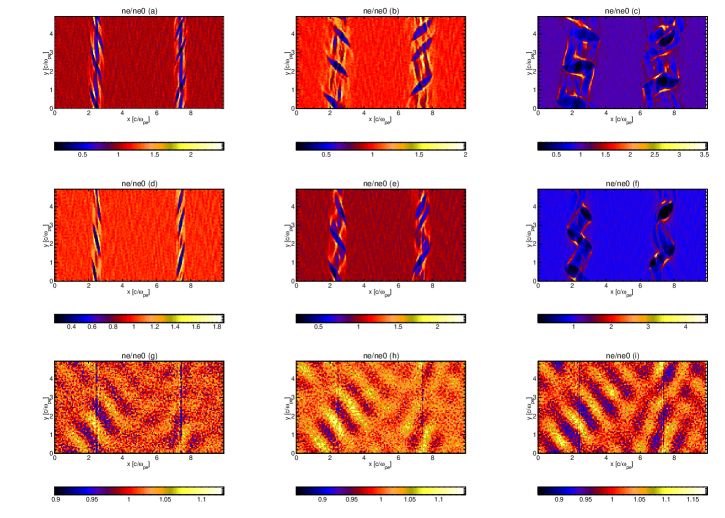
Figure 1: Snapshots of electron number density $n_{\rm e}$. The row of panels (a), (b) and (c) show $n_{\rm e}/n_{0}$ for Run 0 at times $t=20,\;25,\;30/\omega_{\rm pe}$. The row of panels (d), (e) and (f) show $n_{\rm e}/n_{0}$ for Run 2 at times $t=20,\;25,\;30/\omega_{\rm pe}$. The row of panels (g), (h) and (i) show $n_{\rm e}/n_{0}$ for Run 6 at twice the times $t=40,\;50,\;60/\omega_{\rm pe}$. See Table 1 for details.

III.2 Numerical simulation considerations

In this work we use 2.5D version of PIC code EPOCH. This a 1.5, 2.5 and 3D, fully electromagnetic, PIC code [28]. In order to be able to use periodic boundary conditions throughout, which we remark, are the most precise boundary condition for the numerical implementation, we use a "sandwich" with three layers of plasma with the following properties: two down-flow layers satisfying $x/L_{x}<0.25$ or $x/L_{x}>0.75$ with velocity $v_{0}/c=-0.2$ and one up-low layer with $0.25<x/L_{x}<0.75$ with velocity $v_{0}/c=0.2$ in between and $v_{0}$ being parallel to $Oy$ axis. The system size is $(L_{x},L_{y})=(10c/\omega_{\rm pe},5c/\omega_{\rm pe})$ which is resolved with $200\times 100$ grid. This means the each grid cell has a size of 1/20th of $c/\omega_{\rm pe}$, i.e. $\Delta_{x}=\Delta_{y}=0.05c/\omega_{\rm pe}$. Maximal temperature is set as $T_{\rm e,i,max}=m_{e}(0.005c)^{2}/k_{B}=148239.77$ K. This ensures a cold plasma approximation because $v_{\rm th,e}=\sqrt{k_{B}T_{\rm e,i,max}/m_{e}}=0.005c\ll v_{0}=0.2c$. The reason we refer to the maximal temperature is because it actually varies across x-axis. This is because as in Tsiklauri [29] we keep pressure balance by making $p_{\rm e,i}=n_{\rm e,i}(x)kT_{\rm e,i}(x)=const$, i.e. $T_{\rm e,i}(x)=T_{\rm e,i,max}[n_{0}/n_{\rm e,i}(x)]\propto 1/n_{\rm e,i}(x)$. With the magnetic field being uniform $B_{\rm y0}=\bar{B}_{0}B_{\rm MHD}=\bar{B}_{0}\sqrt{\mu_{0}m_{e}n_{e}}v_{0}$, given by equation 13, this means that total initial pressure balance $p_{\rm e,i}+B^{2}/(2\mu_{0})=const$ is satisfied. The factor $\bar{B}_{0}=0,0.5,1.0,5.0,7.5,10.0,15.0$ provides a variation the external magnetic field, $B_{\rm y0}/B_{\rm MHD}=0,\;<1,\;1,\;\gg 1$. The electron and ion number densities are set as:
For the down-lows

$$n_{\rm e,i}(x)=\begin{cases}n_{0},&\text{if }(x<0.25L_{x})\text{ or }(x>0.75L_{x})\\ 10^{-2}n_{0},&\text{otherwise}\end{cases}$$ (28)

For the up-flow, vice versa

$$n_{\rm e,i}(x)=\begin{cases}10^{-2}n_{0},&\text{if }(x<0.25L_{x})\text{ or }(x>0.75L_{x})\\ n_{0},&\text{otherwise}\end{cases}$$ (29)

The factor $10^{-2}$, while drops density to nearly zero, stops EPOCH from slowing down for numerical reasons. In EPOCH code physical quantities are in SI units, so we fix $n_{0}=10^{15}$ particles per m^-3 typical of many collisionless astrophysical plasmas. The terms up-flow and down-flows only refer to motions figurally up and down the $Oy$ axis, as there is no gravity present in our simulations or calculations. The plasma consists of electrons and protons with the realistic mass ration $m_{\rm p}/m_{\rm e}=1836$. Both electrons and ions are mobile throughout the simulation. At $t=0$ electrons and ions velocities are set as descirebed above i.e. a "sandwich" with three layers of plasma. This ensures that initially there is zero net current. In EPOCH implementation we effectively load 4 plasma species, electron and proton up-flows and down-flows as specified by Eqs. 28 and 29. We use 200 particles per cell for each species. so in total, we have $4\times 200\times 200\times 100=1.6\times 10^{7}$ particles. One numerical run takes circa 40 minutes on 12 processor cores. In this paper we only show snapshots of electron number density $n_{e}$ and the generated by ESKHI magnetic field $B_{z}$ component normalized on $B_{\rm MHD}=({m_{e}\omega_{\rm pe}}/{e})({v_{0}}/{c})$. The length is normalized on $c/\omega_{\rm pe}$. The end simulation time is set $150/\omega_{\rm pe}$.

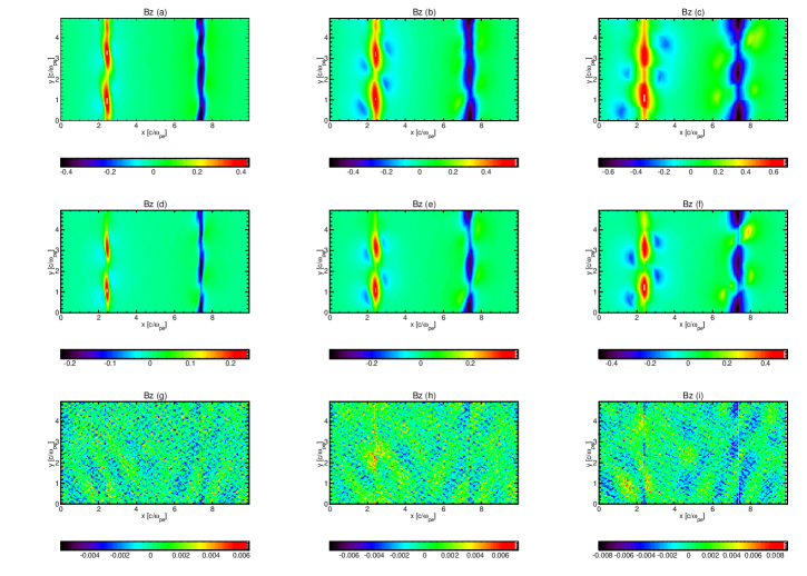
Figure 2: Snapshots of out-of-plane magnetic field $B_{z}$ generated by the ESKHI. The numerical runs and the snapshot times are in direct correspondence to Fig.1.

Table 1: Table of numerical runs considered. See text discussing Fig.3 for the explanation of the notation used.

Run	$\bar{B}_{0}=B_{\rm y0}/B_{\rm MHD}$	$(\Gamma\omega_{\rm pe})_{\rm Diam.}$=r_i[1]	$(\Gamma\omega_{\rm pe})_{\rm Fit}$
0	0.0	0.3667	0.3663
1	0.5	0.3138	0.3061
2	1.0	0.2504	0.2629
3	5.0	0.1340	0.1234
4	7.5	0.0834	0.0927
5	10.0	0.0690	0.0742
6	15.0	0.0668	0.0531

IV The Results

In Fig.1 we show snapshots of electron number density $n_{\rm e}$, which is the sum of down and up flowing electrons. The row of panels (a), (b) and (c) show $n_{\rm e}/n_{0}$ for Run 0 at times $t=20,\;25,\;30/\omega_{\rm pe}$. The row of panels (d), (e) and (f) show $n_{\rm e}/n_{0}$ for Run 2 at times $t=20,\;25,\;30/\omega_{\rm pe}$. The row of panels (g), (h) and (i) show $n_{\rm e}/n_{0}$ for Run 6 at twice the times $t=40,\;50,\;60/\omega_{\rm pe}$. We gather from Fig.1 that in the case zero external magnetic field (Run 0), the elongated, rotating vortices are progressively generated. We note significant similarities of panels corresponding the Run 0 to a similar numerical run with the same number density across the shear interface from Alves et al. [4], see their Figure 6. The vortices start as narrow elongated flow structures with under-dense cores $n_{\rm e}/n_{0}\simeq 0.5$ and strongly over-dense edges $n_{\rm e}/n_{0}\simeq 2$. Note the values on the color bar. As the time progresses from 20 to $30/\omega_{\rm pe}$ the vortex core-edge contrasts deepen even further and the width of vortices grows. Such large values of under- and over-density indicates strongly non-linear evolution of these ESKHI-generated vortices. As the external magnetic field is increased (Run 2) the values of under- and over-density in the vortices drop initially. In the case of $\bar{B}_{0}=B_{\rm y0}/B_{\rm MHD}\gg 1$ (Run 6) vortices disappear altogether and only linear amplitude waves can be seen generated in the vicinity of the shear interfaces $x/L=0.25$ and 0.75. As can be seen in Figure 1, panels (a)–(f), the simulation results are not affected by the periodic boundary conditions used, because across x-axis vortices never reach boundaries, while they simply leave and re-enter at the top and botton boundaries across y-axis.

Fig.2 has a purpose to quantify how the out-of-plane magnetic field $B_{z}$ is generated by the ESKHI. We see in Fig.2 that in the case zero external magnetic field (Run 0) DC (although with a corrugated shape) magnetic field $B_{z}$ is progressively generated in the vicinity of the shear interfaces $x/L=0.25$ and 0.75. The values, judging from the color-bar, range $\pm(0.4-0.6)B_{\rm MHD}$ and they grow as the time progresses from left to right panels. Again we mention that significant similarities can be seen in panels corresponding the Run 0 to a similar numerical run with the same number density across the shear interface from Alves et al. [4], see their Figure 7. For the further increased (increased from zero) external magnetic field, for Run 2, we see that the generated values of $B_{z}$ are about factor of two smaller compared to Run 0. Also gaps in the generated DC field appear, as these structures further narrow down across the shear interfaces at $x/L=0.25$ and 0.75. For Run 6, the values of $B_{z}$ drop to 0.005 near the shear interfaces at $x/L=0.25$ and 0.75.

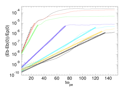
Figure 3: Black, red, green, blue, cyan, gold and thick solid curves show $(E_{B}-E_{B}(0))/E_{p}(0)$ using numerical simulation data from Run0 – Run 6 using Eq.30. The open diamonds with the same multi-colors are showing the fit using Eq.31.

In Fig.3 we show the time evolution of perturbation equipartition energy $(E_{B}-E_{B}(0))/E_{p}(0)$. It is crucial that we subtract $E_{B}(0)$ because we want to separate the pre-existing magnetic field energy contribution from the ESKHI-generated magnetic field energy. We calculate this quantity in the following way: at every time step we load the data and calculate the following quantity:

$$\begin{split}&\frac{E_{B}(t)-E_{B}(0)}{E_{p}(0)}=\\ &\iint\frac{b_{x}(x,y,t)^{2}+[b_{y}(x,y,t)-B_{y0}]^{2}+b_{z}(x,y,t)^{2}}{2\mu_{0}E_{p}(0)}dxdy=\\ &\frac{1}{2\mu_{0}E_{p}(0)}\sum_{i=1}^{n}[b_{x}(x_{i},y_{i},t)^{2}+[b_{y}(x_{i},y_{i},t)-B_{y0}]^{2}+\\ &b_{z}(x_{i},y_{i},t)^{2}]\Delta x\Delta y.\end{split}$$ (30)

Note that in Eq.30 the numerical integration is done by the midpoint rule (also known as the rectangle rule). In Fig.3 black, red, green, blue, cyan, gold and thick solid curves show $(E_{B}-E_{B}(0))/E_{p}(0)$ using numerical simulation data from Run0 – Run 6 using Eq.30. We gather that ESKHI rapidly grows the magnetic perturbation equipartition energy on the time scales of 30 to $120/\omega_{\rm pe}$ depending on the strength of the background external magnetic field. This exponential growth phase is followed by a plateau which as explained by Alves et al. [4] is due to the generated by ESKHI magnetic field component $B_{z}$ blocks the flow of electrons across the shear interfaces at $x/L=0.25$ and 0.75. We also see that as $\bar{B}_{0}=B_{\rm y0}/B_{\rm MHD}$ increases from 0 to 15 the growth rate of ESKHI decreases considerably. The open diamonds of the same color, as stated above, show our fit using the following method. We use Interactive Data Language (IDL)’s built-in function called
r_i=poly_fit( $\omega_{\rm pe}t,$
alog((E_B-E_B(0))/E_p(0)),1,/double), where $i=0,\ldots,6$ for each of the Run0 – Run 6. effectively this function fits a 1st order polynomial to natural logarithm of $(E_{B}-E_{B}(0))/E_{p}(0)$ with $r[0]_{i}$ and $r[1]_{i}$ are the 0th and and 1st order fit coefficients to the polynomial. This fit then enables to plot with open diamonds showing data fit using Eq. 31:

$$e^{r_{i}[0]}\times e^{r_{i}[1]\omega_{\rm pe}t}.$$ (31)

The values of $r_{i}[1]$ are quoted as the 3rd column of Table 1. Effectively these values are the growth rates of ESKHI $(\Gamma\omega_{\rm pe})_{\rm Diam.}$=r_i[1] shown with multi-color open diamonds in Fig.3.

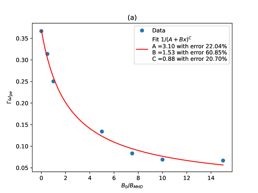
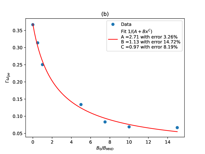
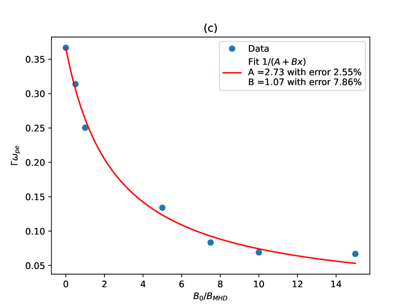
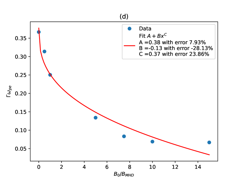
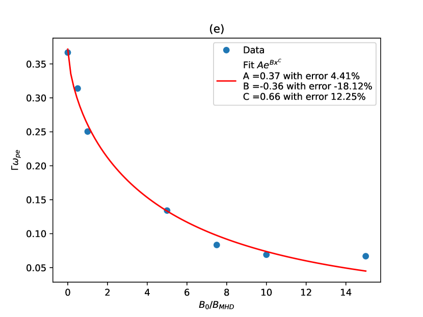
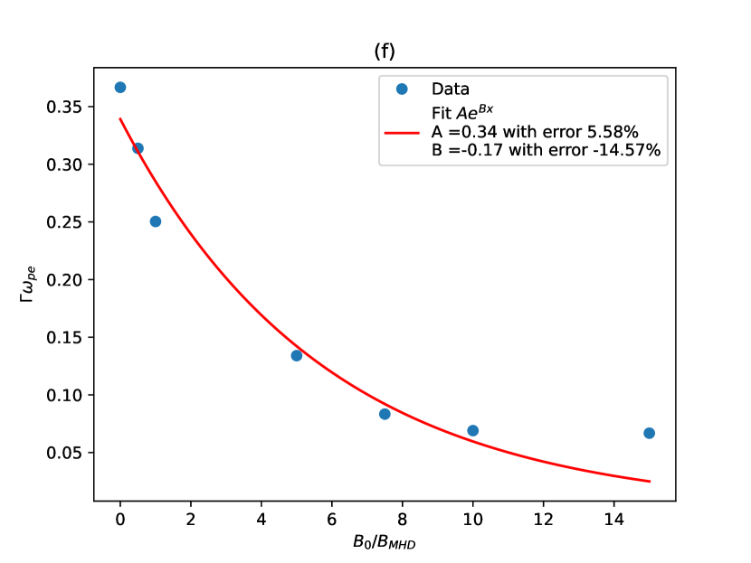
Figure 4: Various plausible functions fitted to $(\Gamma\omega_{\rm pe})_{\rm Diam.}$ values i.e. the best possible functional fit to the 3rd column of Table 1.

In Fig.4 we would like to deduce the effect of external magnetic field on ESKHI in a functional dependence form. In other words, we would like to know what function can be fitted to $(\Gamma\omega_{\rm pe})_{\rm Diam.}$. Various plausible functions were attempted. Only a small fraction of fit functions is shown in panels (a)–(f) in Fig.4. We gather from Fig.4 that in panel (c) we have the best fit with the smallest errors. Thus we conclude that the best fit is hyperbolic, $\Gamma(B_{0})\omega_{\rm pe}=\Gamma_{0}\omega_{\rm pe}/(A+B\bar{B}_{0})$, where $\Gamma_{0}\omega_{\rm pe}=1/\sqrt{8}=0.35$ is the electron scale KHI growth rate without external magnetic field and $\bar{B}_{0}=B_{0}/B_{\rm MHD}$ is the ratio of external and two-fluid MHD stability threshold magnetic field. The hyperbolic fit numerical values of the growth rate are quoted for reference as the 4th column in Table 1. Indeed, as can be deduced both from Fig. 4(c) and the 3d and 4th columns in Table 1, the fit graphically and numerically is rather good. The factor, which is the x-axis in Fig.4 $\bar{B}_{0}=0,0.5,1.0,5.0,7.5,10.0,15.0$ provides a variation the external magnetic field. Paradoxically, for the growth rate predicted by Eq.(26) which is supposed to be the best fit, the fit even does not converge due to large errors.

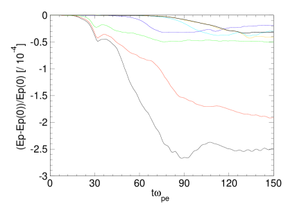
Figure 5: Time evolution of particle perturbation kinetic energy $(E_{p}-E_{p}(0))/E_{p}(0)$ using numerical simulation data from Run 0 – Run 6 with the same multi-color curves as in Fig.3

In Fig.5 we show the time evolution of particle perturbation kinetic energy $(E_{p}-E_{p}(0))/E_{p}(0)$ using numerical simulation data from Run0 – Run 6 with the same multi-color curves as in Fig.3. We deduce two observations from Fig.5: (i) The magnetic field generated by ESKHI comes at an expense of reduction in particle kinetic energy; (ii) The strongest reduction in the kinetic energy is seen for the case of Run 0, a zero background external magnetic field when the ESKHI growth rate is the largest. As the external magnetic field is increased, this arrests the flow of electrons, across the shear interfaces and we see lesser and lesser reduction in the kinetic energy, as a result of this.

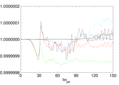
Figure 6: Similar to Figure 5 but now for the total energy.

In Fig.6 we plot the total energy $(E_{p}+E_{f})/(E_{p}(0)+E_{f}(0))$ in a similar manner to Figure 5. Note that $E_{f}$ denotes the total EM field energy, automatically calculated by EPOCH as data.TOTAL_FIELD_ENERGY, which includes contribution from both magnetic and electric fields, while in Fig.3 we had to calculate perturbation equipartition energy $(E_{B}-E_{B}(0))/E_{p}(0)$ manually, using Eq.30. We gather from Fig.6 that the total energy conservation in all our EPOCH numerical runs is superb and the relative errors are contained within a small margin of $\pm 0.0000001$ i.e. $\pm 0.00001\%$.

V Conclusions

ESKHI can be of importance in many collisionless plasmas e.g. when solar wind interacts with planetary magnetospheres, magnetic field is generated in AGN jets, or shocks and flows found in Gamma Ray Bursts [1, 2, 3, 4, 5]. The aim of this paper is to study the effect of external, background magnetic field on ESKHI. Thus we use particle-in-cell, fully electromagnetic plasma simulation as the main tool for this purpose. This study finds that in the kinetic regime, the presence of external magnetic field reduces the growth rate of the instability – a result similar to the well-known analogue – magnetohydrodynamic KHI. While, in MHD there is known threshold magnetic field for KHI stabilization as first shown by Michael [21], for ESKHI this is yet to be determined by an appropriate analytical calculation that would extend approach used in [4, 5] by adding the external, background magnetic field. Such calculation is rather complex if all three components of velocity $v_{x},v_{y},v_{z}$ are considered. Note that in EPOCH in all 1.5, 2.5, 3D versions all three components of velocity are always present. Instead, for the purposes of this paper, we only use the calculations based on Eqs. 21-23, and their outcomes to set the scale of two-fluid MHD stability threshold magnetic field, derived in Appexdix A and given by Eq. 14. As it stands, without a fully kinetic analytical expression for the growth rate, we decided to use several numerical simulation runs to find an empirical dependence of ESKHI growth rate, $\Gamma(B_{0})\omega_{\rm pe}$, on the strength of applied external magnetic field. Our results show that the best fit is hyperbolic, $\Gamma(B_{0})\omega_{\rm pe}=\Gamma_{0}\omega_{\rm pe}/(A+B\bar{B}_{0})$. We note an urgent need for an analytical theory to back up the said growth rate dependence on the external magnetic field. The first peculiar and important result that follows from our study is that in astrophysical objects where a strong magnetic field pre-exists, the generation of an additional magnetic field by the ESKHI is suppressed. The latter suggests that with this, the Nature provides a "safety valve" – natural protection not to "over-generate" magnetic field. The second peculiar result is that we show that two-fluid (nonrelativistic) MHD threshold magnetic field, calculated in Appendix A, (Eq.13 or equally Eq.14) is the same (up to a factor of $\sqrt{\gamma_{0}}\approx~{}1$) as the DC saturation magnetic field, predicted by the fully kinetic theory (Eq.9) established by Grismayer et al. [3], Alves et al. [4].

This work was complete when the author has become aware (G.P. Zank, private communication) of Che and Zank [30]. The calculation shown in our Appendix A and also our Eq.27 appear to be similar to that of Che and Zank [30]. However, it appears that the conclusion of Che and Zank [30], we quote: "The growth rate of the EM mode is $\gamma_{\rm EM}\sim\Omega_{\rm ce}$, which is the electron gyro-frequency" is neither supported by the results of our PIC simulations nor is according to a common sense, because: (i) it is clear that ESKHI exists without magnetic field [3, 4], (ii) $\gamma_{\rm EM}\sim\Omega_{\rm ce}=eB/m_{\rm e}\propto B$ would tend to zero in the absence of the magnetic field. Further analysis is needed to study the differences in the conclusions of this study and Che and Zank [30].

VI Data Availability

The data that support the findings of this study are available from the corresponding author upon reasonable request.

Appendix A Appendixes

Starting with the equations of two-fluid MHD with stationary ions 21–23, we consider two magnetized electron flows with properties $\rho_{e1}$, $p_{e1}$, $U_{e1}$, $B_{1}$ for $y<0$ and $\rho_{e2}$, $p_{e2}$, $U_{e2}$, $B_{2}$ for $y>0$ with the interface at $y=0$. We only consider $xOy$ plane. This calculation extends that of Michael [21] two-fold: (i) we consider situation where bulk flow velocity is replaced by electron velocity, $\vec{v}\to\vec{v}_{e}$ and $\rho\to\rho_{e}$; and (ii) the densities across the interface are different. For $y<0$ we have the following linearized equations in the component form:

$$\frac{\partial b_{x}}{\partial t}+U_{e1}\frac{\partial b_{x}}{\partial x}=B_{1}\frac{\partial v_{ex}}{\partial x},$$ (32)

$$\frac{\partial b_{y}}{\partial t}+U_{e1}\frac{\partial b_{y}}{\partial x}=B_{1}\frac{\partial v_{ey}}{\partial x},$$ (33)

$$\frac{\partial v_{ex}}{\partial t}+U_{e1}\frac{\partial v_{ex}}{\partial x}=-\frac{1}{\rho_{0e1}}\frac{\partial p_{e1}}{\partial x},$$ (34)

$$\frac{\partial v_{ey}}{\partial t}+U_{e1}\frac{\partial v_{ey}}{\partial x}=-\frac{1}{\rho_{0e1}}\frac{\partial p_{e1}}{\partial y}+\frac{B_{1}}{\mu_{0}\rho_{0e1}}\left(\frac{\partial b_{y}}{\partial x}-\frac{\partial b_{x}}{\partial y}\right),$$ (35)

$$\frac{\partial b_{x}}{\partial x}+\frac{\partial b_{y}}{\partial y}=0,\;\;\;\;\;\;\frac{\partial v_{ex}}{\partial x}+\frac{\partial v_{ey}}{\partial y}=0,$$ (36)

where $v_{ex,ey}$ and $b_{x,y}$ are the perturbations of background values of $U_{e1}$ and $B_{1}$. Next, we substitute in Eqs. 32–36 Fourier ansatz of the form $f=\tilde{f}e^{i(kx+\omega t)}$ and omit the tilde signs:

$$i(\omega+kU_{e1})b_{x}=B_{1}ikv_{ex},$$ (37)

$$i(\omega+kU_{e1})b_{y}=B_{1}ikv_{ey},$$ (38)

$$i(\omega+kU_{e1})v_{ex}=-\frac{ik}{\rho_{0e1}}p_{e1},$$ (39)

$$i(\omega+kU_{e1})v_{ey}=-\frac{1}{\rho_{0e1}}\frac{\partial p_{e1}}{\partial y}+\frac{B_{1}}{\mu_{0}\rho_{0e1}}\left(ikb_{y}-\frac{\partial b_{x}}{\partial y}\right),$$ (40)

$$ikb_{x}+\frac{\partial b_{y}}{\partial y}=0,$$ (41)

$$ikv_{ex}+\frac{\partial v_{ey}}{\partial y}=0.$$ (42)

Eqs. 37–42 can be combined into one master equation for $v_{ey}$:

$$\left(\frac{B_{1}^{2}k^{2}}{\mu_{0}\rho_{0e1}}-(\omega+kU_{e1})^{2}\right)\left(k^{2}v_{ey}-\frac{\partial^{2}v_{ey}}{\partial y^{2}}\right)=0.$$ (43)

We seek solutions to Eq. 43 of the form:
for $y<0$ (medium 1) $v_{ey1}=C_{11}e^{ky}+C_{12}e^{-ky}$ and
for $y>0$ (medium 2) $v_{ey2}=C_{21}e^{ky}+C_{22}e^{-ky}$.
For the solutions to remain finite in the limits $y\to\mp\infty$ we have to demand that $C_{12}=C_{21}=0$.

Let $\xi(x,t)$ be displacement of the interface satisfying a condition $\xi\ll 2\pi/k=\lambda$. As in Michael [21], based on the definition $v_{ey1}=\partial\xi/\partial t+U_{e1}{\partial\xi}/{\partial x}$ and $v_{ey2}=\partial\xi/\partial t+U_{e2}{\partial\xi}/{\partial x}$, we demand continuity of ${\partial\xi}/{\partial t}$:

$$\frac{\partial\xi}{\partial t}=v_{ey1}-U_{e1}\frac{\partial\xi}{\partial x}=v_{ey2}-U_{e2}\frac{\partial\xi}{\partial x},$$ (44)

which at the interface $y=0$ yields

$$(\omega+kU_{e1})C_{11}=(\omega+kU_{e2})C_{22}.$$ (45)

We also have to fulfill the condition for the pressure balance $p_{e}+B^{2}/(2\mu_{0})=const$, substituting $p_{e}=p_{e0}+p_{e1}$ and $B=B_{1,2}+b_{1,2}$, at the interface, at a linear order. Omitting the quadratic terms, at the interface $y=0$ we obtain:

$$p_{e1}+\frac{B_{1}b_{x1}}{\mu_{0}}=p_{e2}+\frac{B_{2}b_{x2}}{\mu_{0}}.$$ (46)

Substituting the following quantities for medium 1

$$p_{e1}=\frac{-i(\omega+kU_{e1})\rho_{e1}C_{11}}{k},$$ (47)

$$b_{x1}=\frac{ikB_{1}C_{11}}{(\omega+kU_{e1})},$$ (48)

and similar expressions for medium 2

$$p_{e2}=\frac{i(\omega+kU_{e2})\rho_{e2}C_{22}}{k},$$ (49)

$$b_{x2}=-\frac{ikB_{2}C_{22}}{(\omega+kU_{e2})},$$ (50)

into Eq. 46 and after multiplying both sides by $k$, we obtain:

$$\begin{split}C_{11}&\left(-(\omega+kU_{e1})\rho_{e1}+\frac{B_{1}^{2}k^{2}}{\mu_{0}(\omega+kU_{e1})}\right)=\\ C_{22}&\left((\omega+kU_{e2})\rho_{e2}-\frac{B_{2}^{2}k^{2}}{\mu_{0}(\omega+kU_{e2})}\right).\end{split}$$ (51)

The next step is to make use of Eq. 45 to obtain:

$$\begin{split}&\frac{\left(-(\omega+kU_{e1})\rho_{e1}+\frac{B_{1}^{2}k^{2}}{\mu_{0}(\omega+kU_{e1})}\right)}{(\omega+kU_{e2})}=\\ &\frac{\left((\omega+kU_{e2})\rho_{e2}-\frac{B_{2}^{2}k^{2}}{\mu_{0}(\omega+kU_{e2})}\right)}{(\omega+kU_{e1})}.\end{split}$$ (52)

Further, simple algebra leads us to a quadratic equation

$$\begin{split}&(\rho_{e1}+\rho_{e2})\omega^{2}+2k(U_{e1}\rho_{e1}+U_{e2}\rho_{e2})\omega+\\ &\left[k^{2}\left(U_{e1}^{2}\rho_{e1}+U_{e2}^{2}\rho_{e2}\right)+\frac{B_{1}^{2}k^{2}}{\mu_{0}}+\frac{B_{2}^{2}k^{2}}{\mu_{0}}\right]=0.\end{split}$$ (53)

Eq. 53 is a quadratic equation with respect to $\omega$, which has the solution given by Eq. 24.

References

- Gruzinov [2008] A. Gruzinov, (2008), arXiv:0803.1182 [astro-ph] .
- Alves et al. [2012] E. P. Alves, T. Grismayer, S. F. Martins, F. Fiúza, R. A. Fonseca, and L. O. Silva, The Astrophysical Journal Letters 746, L14 (2012).
- Grismayer et al. [2013] T. Grismayer, E. P. Alves, R. A. Fonseca, and L. O. Silva, Phys. Rev. Lett. 111, 015005 (2013).
- Alves et al. [2014] E. P. Alves, T. Grismayer, R. A. Fonseca, and L. O. Silva, New Journal of Physics 16, 035007 (2014).
- Alves et al. [2015] E. P. Alves, T. Grismayer, R. A. Fonseca, and L. O. Silva, Phys. Rev. E 92, 021101 (2015).
- Miller and Rogers [2016] E. D. Miller and B. N. Rogers, Journal of Plasma Physics 82, 905820205 (2016).
- Yao et al. [2020] P. Yao, H. Cai, X. Yan, W. Zhang, B. Du, J. Tian, E. Zhang, X. Wang, and S. Zhu, Matter and Radiation at Extremes 5, 054403 (2020).
- Mahdavi-Gharavi et al. [2020] M. Mahdavi-Gharavi, H. Mehdian, and K. Hajisharifi, Advances in Space Research 65, 1607 (2020).
- Helmholtz [1868] H. Helmholtz, Monatsberichte der Koniglichen Preussische Akademie der Wissenschaften zu Berlin 23, 215 (1868).
- Thomson [Lord Kelvin] W. Thomson (Lord Kelvin), Philosophical Magazine 42, 362 (1871).
- Delamere et al. [2011] P. A. Delamere, R. J. Wilson, and A. Masters, Journal of Geophysical Research: Space Physics 116 (2011).
- Foullon et al. [2011] C. Foullon, E. Verwichte, V. M. Nakariakov, K. Nykyri, and C. J. Farrugia, The Astrophysical Journal Letters 729, L8 (2011).
- Johnson et al. [2014] J. R. Johnson, S. Wing, and P. A. Delamere, Space Science Reviews 184, 1 (2014).
- Delamere et al. [2021] P. A. Delamere, N. P. Barnes, X. Ma, and J. R. Johnson, Frontiers in Astronomy and Space Sciences 8, 10.3389/fspas.2021.801824 (2021).
- Piran [2005] T. Piran, Rev. Mod. Phys. 76, 1143 (2005).
- Miura and Pritchett [1982] A. Miura and P. L. Pritchett, Journal of Geophysical Research: Space Physics 87, 7431 (1982).
- Liang et al. [2013a] E. Liang, M. Boettcher, and I. Smith, The Astrophysical Journal Letters 766, L19 (2013a).
- Liang et al. [2013b] E. Liang, W. Fu, M. Boettcher, I. Smith, and P. Roustazadeh, The Astrophysical Journal Letters 779, L27 (2013b).
- Nishikawa et al. [2014] K.-I. Nishikawa, P. E. Hardee, I. Dutan, et al., The Astrophysical Journal 793, 60 (2014).
- Nishikawa et al. [2013] K.-I. Nishikawa, P. Hardee, B. Zhang, et al., Annales Geophysicae 31, 1535 (2013).
- Michael [1955] D. H. Michael, Mathematical Proceedings of the Cambridge Philosophical Society 51, 528 (1955).
- Chandrasekhar [1961] S. Chandrasekhar, Hydrodynamic and Hydromagnetic Stability (Dover Publications, Inc., 1961).
- Blandford and Pringle [1976] R. D. Blandford and J. E. Pringle, Monthly Notices of the Royal Astronomical Society 176, 443 (1976).
- Lyutikov [2013] M. Lyutikov, Phys. Rev. E 88, 053103 (2013).
- Gordeev et al. [1994] A. Gordeev, A. Kingsep, and L. Rudakov, Physics Reports 243, 215 (1994).
- Cho and Lazarian [2009] J. Cho and A. Lazarian, The Astrophysical Journal 701, 236 (2009).
- Zhao et al. [2010] J. S. Zhao, J. Y. Lu, and D. J. Wu, The Astrophysical Journal 714, 138 (2010).
- Arber et al. [2015] T. D. Arber, K. Bennett, C. S. Brady, et al., Plasma Physics and Controlled Fusion 57, 1 (2015).
- Tsiklauri [2023] D. Tsiklauri, Monthly Notices of the Royal Astronomical Society 527, 10822 (2023).
- Che and Zank [2023] H. Che and G. P. Zank, Physics of Plasmas 30, 062110 (2023).