Detecting Adversarial Data via Perturbation Forgery

Abstract

As a defense strategy against adversarial attacks, adversarial detection aims to identify and filter out adversarial data from the data flow based on discrepancies in distribution and noise patterns between natural and adversarial data. Although previous detection methods achieve high performance in detecting gradient-based adversarial attacks, new attacks based on generative models with imbalanced and anisotropic noise patterns evade detection. Even worse, existing techniques either necessitate access to attack data before deploying a defense or incur a significant time cost for inference, rendering them impractical for defending against newly emerging attacks that are unseen by defenders. In this paper, we explore the proximity relationship between adversarial noise distributions and demonstrate the existence of an open covering for them. By learning to distinguish this open covering from the distribution of natural data, we can develop a detector with strong generalization capabilities against all types of adversarial attacks. Based on this insight, we heuristically propose Perturbation Forgery, which includes noise distribution perturbation, sparse mask generation, and pseudo-adversarial data production, to train an adversarial detector capable of detecting unseen gradient-based, generative-model-based, and physical adversarial attacks, while remaining agnostic to any specific models. Comprehensive experiments conducted on multiple general and facial datasets, with a wide spectrum of attacks, validate the strong generalization of our method.

Table 1: Properties of our method vs Other Adversarial Detection: We summarize four metrics for adversarial detection. “Detect Attacks” means what kind of attacks the method is designed to detect. “Attack-Agnostic” describes whether the detection can detect unseen attack types. “Model-Agnostic” describes whether the method is independent of the protected model. Finally, “Time Cost” measures the time cost of a detector during inference.

Methods	Detect Attacks	Attack-Agnostic	Model-Agnostic	Time Cost
LID [24]	Gradient	$\times$	$\times$	$\ast$
LiBRe [5]	Gradient	✓	$\times$	$\ast$
EPSAD [47]	Gradient	✓	✓	$\ast\ast$
SPAD [37]	Gradient + GAN	✓	✓	$\ast$
Ours	Gradient + GAN + Diffusion	✓	✓	$\ast$

1 Introduction

Numerous studies have demonstrated the effectiveness of deep neural networks (DNNs) in various tasks [32]. However, it is also well-known that DNNs are vulnerable to adversarial attacks, which generate adversarial data by adding imperceptible perturbations to natural images, potentially causing the model to make abnormal predictions. This vulnerability reduces the reliability of deep learning systems, highlighting the urgent need for defense techniques. Some approaches employ adversarial training techniques [46], which incorporate adversarial data into the training process to inherently bolster the model’s immunity against adversarial noise (adv-noise). Other methods utilize adversarial purification [45] to cleanse the input data of adv-noise before model inference. Unfortunately, adversarial training often results in diminished classification accuracy on adversarial data and may sacrifice performance on natural data. While purification techniques may seem more reliable, the denoising process can inadvertently smooth the high-frequency texture of clean images, leading to suboptimal accuracy on both natural and adversarial images.

Another branch of adversarial defense is adversarial detection [10, 24, 34], which aims to filter out adversarial data before they are fed into target systems. These methods rely on discerning the discrepancies between adversarial and natural distributions, thereby maintaining the integrity of target systems while achieving high performance in defending against adversarial attacks. However, existing adversarial detection approaches primarily train specialized detectors tailored for specific attacks or classifiers [47], which may not generalize well to unseen advanced attacks [39].

Some recent approaches [47, 37] have attempted to enhance the generalization of adversarial detectors by leveraging diffusion models and manually designed pseudo-noise. Nevertheless, as shown in Table 1, this improvement often comes at the cost of increased inference time, and even well-trained detectors still struggle with adversarial data produced by generative models such as generative adversarial networks (GANs) and diffusion models. Specifically, generative-model-based adversarial attacks, such as M3D [48] and Diff-PGD [42], are recently developed techniques designed to generate more natural adversarial data. Unlike traditional gradient-based attacks like PGD [25], generative-model-based attacks tend to create imbalanced and anisotropic perturbations that are intense in high-frequency and salient areas but mild in low-frequency and background areas. These perturbations circumvent all current adversarial detection methods, posing a new challenge to the field. Therefore, there is an urgent need for a low-time-cost detection method with strong generalization performance against both unseen gradient-based attacks and unseen generative-model-based attacks.

In this paper, we investigate the association between the distributions of different adv-noises. As shown in Figure 1, by modeling the noise as Gaussian distributions, we define the proximity relationship of noise distributions in a metric space and establish a perturbation method to construct proximal distributions. Based on these assumptions and definitions, we demonstrate that all adv-noise distributions are proximal using the Wasserstein distance, and we deduce a corollary that an open covering of the adv-noise distributions exists. We then propose the core idea of this paper: by learning to distinguish the open covering of adv-noise distributions from the natural distribution, we obtain a detector with strong generalization performance against all types of unseen attacks.

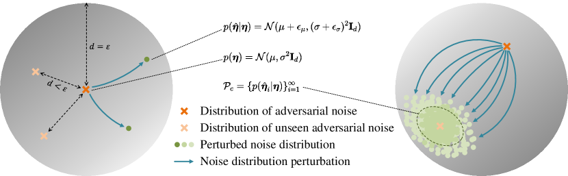
Figure 1: Illustration of the proximity of adversarial noise distributions and perturbed noise distributions. Left: all the distributions of adversarial noise and the perturbed distributions are in a $\epsilon$-ball centered on a given adv-noise distribution. Right: by incessantly perturbing the commonly used adversarial noise distribution, we obtain an open covering of distributions of adversarial noise.

Based on this idea, we propose Perturbation Forgery, a pseudo-adversarial data generation method designed to train a detector with strong generalization capabilities for detecting all types of adversarial attacks. As shown in Figure 2, Perturbation Forgery comprises distribution perturbation, sparse mask generation, and pseudo-adversarial data (pseudo-adv-data) production. By continuously perturbing the noise distribution of a commonly used attack, such as FGSM [12], we obtain a nearly complete family of distributions that form the aforementioned open covering. Simultaneously, sparse masks are generated using attention maps and saliency maps of the natural data, converting the sampled global noises into local forms to help the detector focus on local noise patterns. Sampling noises from the perturbed noise distributions, we sparsify these noises with the sparse masks and inject them into natural data. This process converts half of the natural data into pseudo-adv-data, which are then combined with the remaining uncontaminated data to train the adversarial detector. To the best of our knowledge, we are the first to empower a detector with the robust ability to detect all types of adversarial attacks, including gradient-based, GAN-based, diffusion-based, and physical attacks.

Our contributions are summarized in four thrusts:

$\bullet$ By modeling adversarial noise as Gaussian distributions, we investigate the association between different adversarial noise distributions and demonstrate their proximity in a metric space.

$\bullet$ Based on our assumptions and definitions, we deduce the existence of an open covering for adv-noise distributions and propose training a detector to distinguish this open covering from the natural data distribution, thereby achieving strong generalization.

$\bullet$ Building on our deductions, we propose Perturbation Forgery, which includes distribution perturbation, sparse mask generation, and pseudo-adversarial data production. This method is designed to train a detector with strong generalization performance against all types of unseen attacks, including gradient-based, GAN-based, diffusion-based, and physical adversarial data.

$\bullet$ We conduct evaluations on multiple general and facial datasets across a wide spectrum of gradient-based, generative-model-based, and physical attacks, demonstrating the consistently strong performance of our method in adversarial detection tasks.

2 Related Work

2.1 Adversarial Attack

Gradient-based adversarial attack

Adversarial attacks [12] attempt to fool a classifier into changing prediction results by injecting subtle perturbations to the input data while maintaining imperceptibility from human eyes. By introducing iterative perturbation, PGD [25] and BIM [20] generate adversarial data with significantly improved attack performance, while DIM [41], TIM [7], SIM [22], and VIM [39] improve the transferability under the black-box setting and achieves a high attack rate against several defense techniques. In this paper, a wide spectrum of gradient-based attacks are used to test the detection performance of our method.

Generative-model-based Adversarial Attacks

Recently, another branch of attack uses generative models to make adversarial data with a more natural style and imbalanced noise compared to gradient-based attacks. Among them, CDA [26], TTP [27], and M3D [48] utilize GAN to craft adversarial data and achieve higher efficiency when attacking large-scale datasets. Diff-Attack [1] and Diff-PGD [42] employ the diffusion model as a strong prior to better ensure the realism of generated data. Targeting perturbing facial recognition systems, AdvMakeup [44] and AMT-GAN [16] are presented to generate imperceptible face adversarial images. In this paper, multiple generative-model-based adversarial attacks on ImageNet and facial datasets are used for testing.

2.2 Adversarial Detection

As one of the technical solutions to ensure the safety of DNNs, there has been a significant amount of exploration in the field of adversarial detection [10]. LID [24] is proposed for evaluating the proximity of an input to the natural manifold, while SID [34] can transform the decision boundary by incorporating wavelet transforms. LiBRe [5] leverages Bayesian neural networks to endow pre-trained DNNs with the ability to defend against unseen adversarial attacks. In order to enhance the generalization of detectors, SPAD [37] leverages a data augmentation method to detect adversarial face images, while EPSAD [47] incorporates a diffusion model to detect adversarial data with minimal perturbation magnitude, albeit at the cost of inference time. While current methods have achieved remarkable improvements in adversarial detection, generative-model-based adversarial attacks can easily circumvent them, posing a new challenge. To address the problems above, our method is proposed to detect all types of unseen attacks, including gradient-based, GAN-based, diffusion-based, and physical adversarial data.

3 Proximity of Adversarial Noise Distribution

In this section, we provide an overview of the preliminary concepts related to adversarial data generation and explore the relationship between adversarial noise distributions. We define the proximity of noise distributions and examine the imperceptibility of adversarial noise. Following this, we present the core idea of this paper: by learning to distinguish the open covering of adversarial noise distributions from the natural distribution, we develop a detector with strong generalization capabilities against all types of unseen attacks.

Adversarial data generation

Given a DNN $f$ that works on dataset $\mathcal{D}=\{(\mathbf{x}_{i},y_{i})\}^{n}_{i=1}$ with $(\mathbf{x}_{i}\in\mathcal{X},y_{i}\in\mathcal{C})$ being (sample, ground-truth) pair, an adversarial example $\hat{\mathbf{x}}$ regarding sample $\mathbf{x}$ with perturbation magnitude $\epsilon$ is calculated as:

$$\hat{\mathbf{x}}=\mathop{\mathrm{argmax}}_{\hat{\mathbf{x}}\in\mathbb{B}(\mathbf{x},\epsilon)}\mathcal{L}(f(\mathbf{x}),y),$$ (1)

where $\mathcal{L}$ is some loss function and $\mathcal{B}(\mathbf{x},\epsilon)=\{\mathbf{x^{\prime}}|\ell^{p}(\mathbf{x},\mathbf{x^{\prime}})<\epsilon\}$ restricts the perturbation under $\ell^{p}$ norm. Following [12], we simply denote adversarial sample as $\hat{\mathbf{x}}=\mathbf{x}+\boldsymbol{\eta}$.

Proximity of noise distribution

Due to the subtle and imperceptible nature of adv-noise, adversarial data and natural data appear visually similar. Thus, we assume that this similarity also exists between the noises of different adversarial attacks. To investigate the similarity of these noises, we provide the following definition, which depicts a close relationship between two independent noise distributions:

Definition 1 (Proximal Noise Distribution).

Let $P$ and $Q$ be the distribution functions of two independent noise samples $\mathbf{x}_{1}$ and $\mathbf{x}_{2}$. We call them proximal noise distributions if we have a metric $d(\cdot,\cdot)$ and $\exists\ \varepsilon>0$, s.t.

$$d(P,Q)<\varepsilon.$$ (2)

Following out-of-distribution detection methods [8], we assume noise r.v $\boldsymbol{\eta}$ satisfied truncated normal distribution $\mathcal{N}(\mu,\sigma^{2}\mathbf{I}_{d})$ with it’s truncated interval is $[-\epsilon,\epsilon]^{d}$. Built upon Definition 1, we derive the following theorem about the association between the distributions of different adv-noises:

Theorem 1.

Let $\mathcal{P}_{a}$ be the distribution set composed of all the adversarial noise distributions. Given independent noise distributions $Q_{i},i\in N^{+}$. For $\forall\ i\neq j$, $Q_{i}$ and $Q_{j}$ are proximal noise distributions if the following conditions are met.

1) if $Q_{i},Q_{j}\in\mathcal{P}_{a}$.

2) if $\exists\ \epsilon_{\mu},\epsilon_{\sigma}>0$ s.t. $\|\mu_{i}-\mu_{j}\|<\epsilon_{\mu}$ and $|\sigma_{i}-\sigma_{j}|<\epsilon_{\sigma}$ where the $\|\cdot\|$ is a Euclidean norm on $\mathbb{R}^{n}$.

Theorem 2 tells us: 1) All adversarial noise distributions are proximal noise distributions. 2) If the parameters of two noise distributions are sufficiently close to those of a given distribution, we can regard these two distributions as proximal noise distributions.

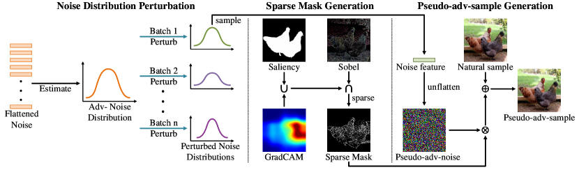
Figure 2: Illustration of Perturbation Forgery. Before training, we estimate the noise distribution of a commonly used attack and continuously perturb it in each batch. After that, we sample noises from the perturbed distribution and convert them into local noise using sparse masks. Finally, pseudo-adversarial data is generated by adding these local noises to the natural samples.

We can further deduce several corollaries of the theorem. 1) All noise distributions proximal to the known adversarial distribution $p(\boldsymbol{\eta})$ form an open $\varepsilon$-ball centered on $p(\boldsymbol{\eta})$, denoting as $\mathcal{P}_{\varepsilon}=\{p(\boldsymbol{\eta}_{i})|d(p(\boldsymbol{\eta}_{i}),p(\boldsymbol{\eta}))<\varepsilon)\}$, and also form a metric space $(\mathcal{P}_{\varepsilon},d)$. 2) The adv-noise distribution set is also located in this ball: $\mathcal{P}_{a}\subset\mathcal{P}_{\varepsilon}$. 3) Based on the properties of the metric space $(\mathcal{P}_{\varepsilon},d)$, for all subset $\mathcal{P}_{i}\subset\mathcal{P}_{\varepsilon}$, there exists an open covering of the subset: $\mathcal{P}_{i}\subset\{G_{c}\}_{c\in J}$.

Based on the corollaries, we deduce the core idea of this paper: Let $p(\hat{\boldsymbol{\eta}}_{i}|\boldsymbol{\eta})=\mathcal{N}(\mu+\epsilon_{\mu i},(\sigma+\epsilon_{\sigma i})^{2}\mathbf{I}_{d}),i=1,2,\dots,n$ denote generated proximal noise distributions of the given adv-noise distribution $p(\boldsymbol{\eta})=\mathcal{N}(\mu,\sigma^{2}\mathbf{I}_{d})$ where $\epsilon_{\mu i},\epsilon_{\sigma i}$ are randomly sampled from uniform distributions and restricted by $\epsilon_{\mu i},\epsilon_{\sigma i}<\varepsilon$. As shown in Figure 1, when $n\rightarrow\infty$, we can always obtain a distribution set $\mathcal{P}_{c}=\{p(\hat{\boldsymbol{\eta}}_{i}|\boldsymbol{\eta})\}_{i=1}^{\infty}$ that forms an open covering of the adversarial distribution set $\mathcal{P}_{a}$. Trained on the open covering, the detector can distinguish the distributions of natural data and adversarial data, thereby having the functionality to detect unseen adversarial attacks.

4 Perturbation Forgery

Based on the theory support in the last section, we heuristically propose Perturbation Forgery to train a detector with strong generalization against all types of unseen attacks. As illustrated in Figure 2, Perturbation Forgery encompasses three elements: distribution perturbation (Section 4.1), sparse mask generation (Section 4.2), and pseudo-adversarial data production (Section 4.3).

At first, the noise distribution of a commonly used attack is continuously perturbed into numerous noise distributions that remain proximal to the original, thereby forming the open covering. After that, we sample noises from the perturbed distribution and convert them into sparse local noise using sparse masks. Subsequently, pseudo-adversarial data is produced by adding these sparse local noises to natural data. Following [37], we convert half of the natural data into pseudo-adversarial data and train a detector on this pseudo-adversarial data along with the remaining natural data.

4.1 Noise Distribution Perturbation

Given the training dataset $\{(\mathbf{x}_{k},y_{k})\}^{n}_{k=1}$ composed by natural data, we attack on it and generate adversarial noise features $\{\mathbf{z}_{k}=h(\boldsymbol{\eta}_{k})\}_{k=1}^{n}$ by

$$\boldsymbol{\eta}_{k}=\operatorname{Attack}(\mathbf{x})-\mathbf{x},\ k\in[1,n],$$ (3)

where $\operatorname{Attack}(\cdot)$ is a commonly used adversarial attack such as FGSM, and $h:\mathcal{X}\rightarrow\mathbb{R}^{d}$ is the flattening operation that converts multidimensional data into vectors.

Assuming the noise features form a multivariate Gaussian distribution $p(\mathbf{z})=\mathcal{N}(\boldsymbol{\mu},\boldsymbol{\Sigma})$ [8], we estimate the parameters mean $\boldsymbol{\mu}$ and covariance $\boldsymbol{\Sigma}$ of $\mathcal{D}_{\mathrm{noise}}$ by

$$\widehat{\boldsymbol{\mu}}=\frac{1}{N}\sum_{k}\mathbf{z}_{k},\quad\widehat{\boldsymbol{\Sigma}}=\frac{1}{N}\sum_{k}\left(\mathbf{z}_{k}-\widehat{\boldsymbol{\mu}}\right)\left(\mathbf{z}_{k}-\widehat{\boldsymbol{\mu}}\right)^{\top}.$$ (4)

Algorithm 1 Training Procedure with Perturbation Forgery

Input: Training dataset, initial attack $\operatorname{Attack}$, saliency detection model $f_{s}$, and GradCAM model $f_{c}$.
Output: A detector with strong generalization capabilities against all types of unseen attacks.

1:  Generate adversarial noise using the initial attack $\operatorname{Attack}$ in Eq. 3.

2:  Estimate a multivariate Gaussian distribution $p(\mathbf{z})=\mathcal{N}(\widehat{\boldsymbol{\mu}},\widehat{\boldsymbol{\Sigma}})$ of adv-noise using Eq. 4.

3:  for batch $i$ in $1,\cdots,n$ do

4:     Generate a perturbed noise distribution $p(\mathbf{z}_{i})=\mathcal{N}(\widehat{\boldsymbol{\mu}}_{i},\widehat{\boldsymbol{\Sigma}}_{i})$ using Eq. 5.

5:     for sample $\mathbf{x}_{i,k}$ half of batch $i$ do

6:        Generate sparse masks $\operatorname{Mask}(\mathbf{x}_{i,k})$ using Eq. 8.

7:        Sample pseudo-adversarial noise $\widehat{\boldsymbol{\eta}}_{i,k}$ using Eq. 9.

8:        Generate pseudo-adversarial data $\widehat{\mathbf{x}}_{i,k}$ using Eq. 10.

9:     end for

10:     Train the detector on batch $i$.

11:  end for

For the $i^{\mathrm{th}}$ batch of training, we perturb the estimated distribution to a proximal noise distribution by

$$\widehat{\boldsymbol{\mu}}_{i}=\widehat{\boldsymbol{\mu}}+\alpha_{i}\cdot\boldsymbol{m}_{i},\quad\widehat{\boldsymbol{\Sigma}}_{i}=\widehat{\boldsymbol{\Sigma}}+\beta_{i}\cdot\boldsymbol{V}_{i},$$ (5)

where $\boldsymbol{m}_{i}\sim\mathcal{N}(0,\mathbf{I}_{d})$ and $\boldsymbol{V}_{i}\sim\mathcal{N}(0,\mathbf{I}_{d\times d})$ are perturbation vector and perturbation matrix. $\alpha_{i}\sim\boldsymbol{U}(-\epsilon_{\mu},\epsilon_{\mu})$ and $\beta_{i}\sim\boldsymbol{U}(0,\epsilon_{\sigma})$ are scale parameters sampled from uniform distributions. After $n$ batches of training, we have a perturbed distribution set $\{\mathcal{N}(\widehat{\boldsymbol{\mu}}_{i},\widehat{\boldsymbol{\Sigma}}_{i})\}$, thereby forming the approximate closure $\mathcal{P}_{c}$.

4.2 Sparse Mask Generation

Unlike gradient-based adversarial samples, generative-model-based attacks tend to generate imbalanced and anisotropy perturbations, showing much intensity in high-frequency and salient areas and mild in low-frequency and background areas. Besides, in the physical situation, adversarial attacks also tend to add patches to local areas. Noticing this, we propose sparse masks to perturbation forgery to assist the detector in detecting local adv-noises.

Previous research has demonstrated that the spectra of real and fake images differ significantly in high-frequency regions [23]. Additionally, GAN-based adversarial samples data manipulate characteristics, such as abnormal color aberrations, in these high-frequency regions [37]. Given this, we first mask the high-frequency area of a natural sample using saliency detection [29] and GradCAM [30]:

$$\operatorname{Mask}_{1}(\mathbf{x})=\operatorname{Map}(f_{s}(\mathbf{x});\gamma_{s})\cup\operatorname{Map}(f_{c}(\mathbf{x});\gamma_{c}),$$ (6)

where $f_{s}$ and $f_{c}$ are the saliency detection model and GradCAM model respectively. $\operatorname{Map}(\mathbf{x};\gamma)$ is a binary indicator function parameterized by $\gamma$:

$$\operatorname{Map}(\mathbf{x};\gamma)=\operatorname{Clip}_{[0,1]}(\mathbf{x}-\gamma\mathbf{I}_{\mathcal{X}}).$$ (7)

The noise that occurs in the high-frequency region tends to capture only a small part of the region rather than occupying the entire high-frequency spectrum. Therefore, we select the high-frequency point using the Sobel operator [9] to sparsify the mask of sample $\mathbf{x}_{i,k}$:

$$\operatorname{Mask}_{2}(\mathbf{x})=\operatorname{Map}(\operatorname{Sobel}(\mathbf{x});\gamma_{l}),\quad\operatorname{Mask}(\mathbf{x}_{i,k})=\operatorname{Mask}_{1}(\mathbf{x}_{i,k})\cap\operatorname{Mask}_{2}(\mathbf{x}_{i,k}).$$ (8)

4.3 Pseudo-Adversarial Data Production

For the $i^{\mathrm{th}}$ batch of training, we sample pseudo-adversarial noise from the perturbed distribution by:

$$\widehat{\boldsymbol{\eta}}_{i,k}=h^{-1}(\mathbf{z}_{i,k}),\quad\mathbf{z}_{i,k}\in\{\mathbf{z}_{k}|\mathbf{z}_{k}\sim\mathcal{N}(\widehat{\boldsymbol{\mu}}_{i},\widehat{\boldsymbol{\Sigma}}_{i})\ \mathrm{and}\ p(\mathbf{z}_{k})<\gamma_{p}\}$$ (9)

where $h^{-1}:\mathbb{R}^{d}\rightarrow\mathcal{X}$ is an inverse function of $h$ to unflatten noise features, and $\gamma_{p}$ is a threshold that excludes data with a low likelihood. Note that $\boldsymbol{\eta}_{i}$ is a global noise and needs to be localized by a sparse mask. For natural data $\mathbf{x}_{i,k}$ in the $i^{\mathrm{th}}$ batch, the corresponding pseudo-adversarial data $\widehat{\boldsymbol{x}}_{i,k}$ is produced by adding the masked local noise to it:

Table 2: Comparison of AUC scores (%) of detecting gradient-based attacks on ImageNet100.

Detector	BIM	PGD	RFGSM	DIM	MIM	NIM	VNIM	SNIM
LID [24]	0.6838	0.6750	0.6687	0.6943	0.7138	0.5991	0.6847	0.6171
LiBRe [5]	0.7274	0.7149	0.7069	0.7145	0.7708	0.7020	0.7584	0.7191
EPSAD [47]	0.6792	0.6909	0.6902	0.6623	0.7017	0.7070	0.6733	0.6928
SPAD [37]	0.9346	0.9352	0.9329	0.9351	0.9304	0.9422	0.9395	0.9360
ours	0.9911	0.9912	0.9911	0.9863	0.9931	0.9934	0.9878	0.9914

$$\widehat{\mathbf{x}}_{i,k}=\mathbf{x}_{i,k}+\widehat{\boldsymbol{\eta}}_{i,k}\otimes\operatorname{Mask}(\mathbf{\mathbf{x}_{i,k}}).$$ (10)

where $\otimes$ is Hadamard product.

For each batch, we convert half of the natural data to pseudo-adversarial data by Perturbation Forgery and train a binary detector using the Cross-Entropy classification loss. The overall training procedure with Perturbation Forgery is presented in Algorithm 1.

5 Experiments

To validate the detection performance of our approach against various adversarial attack methods, we conduct extensive empirical studies on multiple general and facial datasets. In this section, we provide experimental settings (Section 5.1), compare our method with state-of-the-art detection approaches across three research fields (Sections 5.2, 5.3, and 5.4), and conduct various ablation studies and analyses to further understand our approach (Section 5.5).

5.1 Experiment Settings

Datasets and Network Architectures

The datasets for evaluation include 1) general dataset ImageNet100 [3], and 2) face datasets: Makeup [13], CelebA-HQ [17], and LFW [11]. Gradient-based attacks are executed on ImageNet100, while generative-model-based attacks are launched only on ImageNet100. For face attacks, we conduct Adv-Makeup on the Makeup dataset, AMT-GAN on the CelebA-HQ dataset, and physical attacks on the LFW dataset.

Adversarial Attacks

We adopt 9 gradient-based attacks, 5 generative-model-based attacks, and 6 face attacks to evaluate our method. For gradient-based attacks, FGSM [12] is used as the initial attack to generate the adv-noises, and 8 attacks including BIM [20], PGD [25], RFGSM [36], MIM [6], DIM [41], NIM [22], VNIM [39], and SNIM [22] are used as the unseen attacks. For generative-model-based attacks, we adopt 3 GAN-based attacks including CDA [26], TTP [27], and M3D [48], and 2 Diffusion-model-based attacks including Diff-Attack [1] and Diff-PGD [42] to craft adv-samples. For face attacks, 1 gradient-based attack TIPIM [43], two GAN-based attacks including AdvMakeup [44] and AMT-GAN [16], and 3 physical attacks including Adv-Sticker [35], Adv-Glasses [31], and Adv-Mask [35] produce adversarial face samples. For each of the above attack methods, adversarial data is generated with the perturbation magnitude of $\epsilon=4/255$ (except for the unrestricted attacks) following [47].

Baselines

We compare our method with state-of-the-art detection methods across three research fields, including adversarial detection, synthetic image detection, and face forgery detection, evaluating the detection of various types of adversarial attacks. For detecting gradient-based attacks, we compared our method with adversarial detection methods including LID [24], LiBRe [5], SPAD [37], and EPSAD[47]. Since existing adversarial detection methods do not address generative-model-based adversarial data, we compared our method with synthetic image detection methods including CNN-Detection[38], LGrad[33], Universal-Detector[28], and DIRE[40] for detecting generative-model-based attacks. For detecting GAN-based face attacks, we compared with face forgery detection methods including Luo et al. [23], He et al. [15], and ODIN [21]. We conducted experiments using the pre-trained models and authors’ implementation code of the above methods.

Table 3: Comparison of AUC scores of detecting generative-model-based attacks on ImageNet100.

Detector	CDA	TTP	M3D	Diff-Attack	Diff-PGD
CNN-Detection [38]	0.7051	0.6743	0.6917	0.3963	0.526
LGrad [33]	0.6144	0.6077	0.6068	0.5586	0.5835
Universal-Detector [28]	0.7945	0.8170	0.8312	0.9202	0.5531
DIRE [40]	0.8976	0.9097	0.9129	0.9097	0.9143
EPSAD	0.9674	0.6997	0.7265	0.4700	0.1507
SPAD	0.9385	0.9064	0.8984	0.8862	0.8879
ours	0.9878	0.9678	0.9364	0.9223	0.9223

Table 4: Comparison of AUC scores for detecting various adversarial attacks on the face.

Detector	TIPIM	Adv-Sticker	Adv-Glasses	Adv-Mask	Detector	Adv-Makeup	AMT-GAN
LID	0.6974	0.5103	0.6472	0.5319	He et al. [15]	0.5252	0.8823
LiBRe	0.5345	0.9739	0.8140	0.9993	Luo et al. [23]	0.6178	0.6511
EPSAD	0.8442	0.7446	0.5026	0.3478	ODIN[21]	0.6325	0.6970
SPAD	0.9256	0.9975	0.9244	0.9863	SPAD	0.9657	0.8969
ours	0.9885	0.9999	0.9999	0.9999	ours	0.9762	0.9216

Evaluation Metrics

Following previous adversarial detection works [47], we employ the Area Under the Receiver Operating Characteristic Curve (AUC) as the primary evaluation metric to assess the performance of our classification models. The AUC is a widely recognized metric in the field of machine learning and is particularly useful for evaluating binary classification problems. For fair comparisons, the number of natural data and adversarial data in the experiments remained consistent.

Implementation details

XceptionNet [2] is selected as our backbone model and is trained on all the above datasets. For adv-noise distribution estimation, we utilize Torchattacks [18] to generate 1000 noise images for each dataset. Parameters of uniform distributions are set as $\epsilon_{\mu}=3$ and $\epsilon_{\sigma}=0.005$. The thresholds of sample controlling is set as $\gamma_{s}=0.05$. Thresholds of binary indicator function are set as $\gamma_{s}=0$, $\gamma_{c}=125$ and $\gamma_{l}=100$. Training epochs are set to 10 and convergence is witnessed.

5.2 Detecting Gradient-based Attacks

We begin by comparing our method with state-of-the-art techniques for detecting gradient-based attacks on ImageNet100. All the attacks are seen to LID but unseen to other baselines and our method. For each attack, 1,000 adversarial samples are generated under the white-box setting to test the detection models. All the baseline methods are sourced from existing adversarial detection research. As reported in Table 2, our method demonstrates effective detection (achieving an AUC score over 0.99) across a variety of attack methods, consistently outperforming the baseline approaches. These results validate our assumptions of the noise distribution proximity. By incessantly perturbing the estimated noise distribution of a given attack (FGSM), we obtain an open covering noise of distributions from all the attacks. The consistent detection performance verifies the effectiveness of our core idea to train a detector to distinguish the open covering of adv-noise distributions from natural ones, and demonstrates the strong generalization capability of our method against gradient-based attacks. Additional results for CIFAR10 [19] are provided in Supplementary Material.

5.3 Detecting Generative-model-based Attacks

To investigate the advantage of our method in detecting generative-model-based attacks, we make comparisons with state-of-the-art methods of synthetic image detection and adversarial detection methods on ImageNet100. As shown in Table 3, our method substantially surpasses other methods, exhibiting highly effective detection capabilities. For adversarial detection baselines, due to the noise produced by generative models tending to be imbalanced compared to perturbations of traditional gradient-based attacks, these methods struggle to conduct effective detection. In contrast, with the assistance of sparse masks, our detector can perceive the local noises made by both GAN and diffusion models. As adversarial data is crafted from natural data, most synthetic image detection methods lose their effectiveness except DIRE[40]. It is probably because DIRE leverages the reconstruction error of images generated by diffusion models, thereby maintaining a certain level of effectiveness.

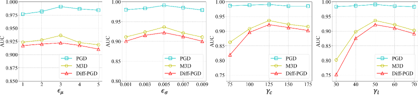
Figure 3: The influence of parameters on the detection performance.

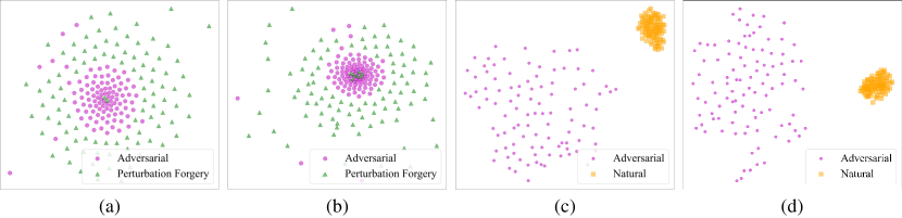
Figure 4: 2D T-SNE visualizations. (a) CIFAR10 flattened noise of adversarial data and Perturbation Forgery. (b) ImageNet100 flattened noises of adversarial data and Perturbation Forgery. (c) CIFAR10 features extracted by the model trained with Perturbation Forgery. (d) ImageNet100 features extracted by the model trained with Perturbation Forgery.

5.4 Detecting Face Adversarial Samples

Adversarial attack on the face recognition model is an important branch of adversarial example research. Therefore, the detection ability of face adversarial samples is an important indicator of the performance of the detector. We conduct various adversarial face attacks and compare our approach with state-of-the-art methods from adversarial face detection and face forgery detection. As shown in Table 4, our method demonstrates excellent performance against a variety of adversarial attacks targeting faces and surpasses many existing adversarial face detection techniques. This further indicates that the sparse mask captures the essential characteristics of adversarial samples and it is a method with strong generalization capabilities for simulating adversarial samples.

5.5 Ablation Study and Analysis

To further evaluate our method, we conduct ablation studies on the proposed sparse mask and the impact of parameters. We also analyze the functionality of Perturbation Forgery through visualizations.

Impact of each mask

As argued, the sparse mask is proposed to assist the detector in identifying local adversarial noises present in generative-model-based adversarial data. As shown in Table 5, the absence of the saliency detection model $f_{s}$ or the GradCAM model $f_{c}$ has little effect on the overall system. This is because the regions masked by $f_{s}$ and $f_{c}$ are somewhat complementary. However, without the Sobel operation to make the mask sparse, the detector fails entirely in detecting attacks, except for CDA, because the noise in generative-model-based adversarial data tends to be

Table 5: Ablation study on masks.

Ablation	CDA	TTP	M3D	Diff-Attack	Diff-PGD
w/o $f_{s}$	0.9755	0.9585	0.9320	0.9197	0.9135
w/o $f_{c}$	0.9864	0.9510	0.9262	0.9031	0.9062
w/o $\operatorname{Sobel}$	0.9868	0.7235	0.6984	0.5231	0.5547

imbalanced and localized, whereas the noise in CDA is more global. Without the sparsification provided by the Sobel operation, the generated pseudo-noise becomes too dense, preventing the detector from effectively focusing on local noise.

Impact of Parameters

We select typical attacks and present curves in Figure 3 to depict the impact of parameters on the detection performance. Parameters $\epsilon_{\mu}$ and $\epsilon_{\sigma}$ have little effect on detecting PGD, while $\gamma_{c}$ and $\gamma_{l}$ have significant effects on detecting M3D and Diff-PGD. This might be because, regardless of whether $\epsilon_{\mu}$ and $\epsilon_{\sigma}$ are large or small, the accuracy of forming the open coverage remains unaffected as long as the data is sufficient. However, too small thresholds lead to adding pseudo-noise to insensitive and low-frequency regions, while too large thresholds result in extremely sparse pseudo-noise that is far from the adversarial noise distribution.

Functionality of Perturbation Forgery

To validate the functionality of our method, we extract features and flattened noises from adversarial data and Perturbation Forgery and visualize them using 2D t-SNE projection. All the adversarial data comes from an unseen adversarial attack. As shown in Figure 4 (a) and (b), by incessantly perturbing the adversarial noise distribution of a commonly used attack, Perturbation Forgery forms an open covering of noises from unseen attacks. Individual samples float outside of the collective because they are outliers from the noise distribution. As shown in Figure 4 (c) and (d), by learning to separate natural data from those generated by Perturbation Forgery, the trained detector can effectively distinguish between natural and adversarial data.

6 Conclusion

In this paper, we explore and define the proximity relationship between adversarial noise distributions by modeling these distributions as multivariate Gaussian. Based on our assumptions and definitions, we establish a perturbation method to craft proximal distributions from a given distribution and demonstrate the existence of an open covering of adversarial noise distributions. After that, we propose the core idea of obtaining a detector with strong generalization abilities against all types of adversarial attacks by learning to distinguish the open covering from the distribution of natural data. Based on this insight, we heuristically propose Perturbation Forgery, which includes noise distribution perturbation, sparse mask generation, and pseudo-adversarial data production, to train an adversarial detector capable of detecting unseen gradient-based, generative-model-based, and physical adversarial attacks, agnostic to any specific models. The major limitation of our method is that finding the optimal scale parameters for distribution perturbation is challenging. We have to rely on continuous experimentation to determine these parameters. However, even if these parameters are not optimal, our method still maintains consistent detection performance across various attacks on multiple general and facial datasets, with a satisfactory inference time cost. Extensive experiments verify the effectiveness of our assumptions and motivations and demonstrate the strong generalization ability of our method against unseen adversarial attacks.

Appendix A Proofs in Section 3

Theorem 2.

Let $\mathcal{P}_{a}$ be the distribution set composed of all the adv-noise distributions. Given independent noise distributions $Q_{i},i\in N^{+}$. For $\forall\ i\neq j$, $Q_{i}$ and $Q_{j}$ are proximal noise distributions if the following conditions are met.

1) if $Q_{i},Q_{j}\in\mathcal{P}_{a}$.

2) if $\exists\ \epsilon_{\mu},\epsilon_{\sigma}>0$ s.t. $\|\mu_{i}-\mu_{j}\|<\epsilon_{\mu}$ and $|\sigma_{i}-\sigma_{j}|<\epsilon_{\sigma}$ where the $\|\cdot\|$ is a Euclidean norm on $\mathbb{R}^{n}$.

Proof.

Denoting the distribution of natural sample $\mathbf{x}$ as $P$, we use the 1-Wasserstein distance as the metric $d(\cdot,\cdot)$, to prove the theorem.

1) We denote the independent adv-noise distribution of $\eta_{i}$ as $Q_{i}\in\mathcal{P}_{a}$ where $\eta_{i}=\hat{\mathbf{x}}_{i}-\mathbf{x}$, and a zero-distribution as $P$ where its mean and variance are zero vectors. Then the 1-Wasserstein distance between $\eta_{i}$ and $\eta_{j}$ can be bound by its metric property and dual form:

$$W_{1}\left(Q_{i},Q_{j}\right) \leq W_{1}(Q_{i},P)+W_{1}(Q_{j},P)$$

$$\leq\sup_{\|g\|_{L}\leq 1}\mathbb{E}_{\boldsymbol{\eta}_{i}\sim Q_{i}}[g(\boldsymbol{\eta}_{i})]-\mathbb{E}_{\mathbf{x}\sim P}[g(\mathbf{x})]+\sup_{\|g\|_{L}\leq 1}\mathbb{E}_{\boldsymbol{\eta}_{j}\sim Q_{j}}[g(\boldsymbol{\eta}_{j})]-\mathbb{E}_{\mathbf{x}\sim P}[g(\mathbf{x})]$$

$$\leq 2\epsilon,$$

where $\|g\|_{L}$ is the Lipschitz constant of function $g$ w.r.t. the norm induced by the metric here.

2) Consider two random noise $\boldsymbol{\eta}_{i}\sim\mathcal{N}_{i}(\mu_{i},\sigma_{i}^{2}\mathbf{I}_{d})$ and $\boldsymbol{\eta}_{j}\sim\mathcal{N}_{j}(\mu_{j},\sigma_{j}^{2}\mathbf{I}_{d})$. While it’s mean and variance satisfied that $\|\mu_{i}-\mu_{j}\|\leq\epsilon$ and $|\sigma_{i}-\sigma_{j}|\leq\epsilon$. then the 2-Wasserstein distance between $\eta_{1}$ and $\eta_{2}$ is

$$W_{2}\left(\boldsymbol{\eta}_{i},\boldsymbol{\eta}_{j}\right)^{2} =\left\|\mu_{i}-\mu_{j}\right\|^{2}+\operatorname{trace}\left(\sigma_{i}^{2}\mathbf{I}_{d}+\sigma_{j}^{2}\mathbf{I}_{d}-2\left((\sigma_{j}^{2}\mathbf{I}_{d})^{1/2}\sigma_{i}^{2}\mathbf{I}_{d}(\sigma_{j}^{2}\mathbf{I}_{d})^{1/2}\right)^{1/2}\right)$$

$$\leq\epsilon_{\mu}^{2}+d\cdot\epsilon_{\sigma}^{2},$$

where $(\sigma_{i}^{2}\mathbf{I}_{d})^{1/2}$ denotes the principal square root of $\sigma_{i}^{2}\mathbf{I}_{d}$. ∎

Corollary 1.

1) All noise distributions proximal to the known adversarial distribution $p(\boldsymbol{\eta})$ form an open $\varepsilon$-ball centered on $p(\boldsymbol{\eta})$, denoting as $\mathcal{P}_{\varepsilon}=\{p(\boldsymbol{\eta}_{i})|d(p(\boldsymbol{\eta}_{i}),p(\boldsymbol{\eta}))<\varepsilon)\}$, and also form a metric space $(\mathcal{P}_{\varepsilon},d)$.

2) The adv-noise distribution set is also located in this ball: $\mathcal{P}_{a}\subset\mathcal{P}_{\varepsilon}$.

3) Based on the properties of the complete metric space $(\mathcal{P}_{\varepsilon},d)$, for all subset $\mathcal{P}_{i}\subset\mathcal{P}_{\varepsilon}$, there exists a finite open covering of the subset: $\mathcal{P}_{i}\subset\{G_{c}\}_{c\in J}$.

Proof.

1) Consider 1-Wasserstein distance as metric $d$, for $\forall Q_{i},Q_{j}\in\mathcal{P}_{\varepsilon}$, we have

$$W_{1}\left(Q_{i}\right)\geq 0.\quad W_{1}\left(Q_{i},Q_{j}\right)=0ifandonlyifQ_{i}=Q_{j}.$$ (11)

$$W_{1}\left(Q_{i},Q_{j}\right)=W_{1}\left(Q_{j},Q_{i}\right).$$ (12)

$$W_{1}\left(Q_{i},Q_{j}\right)\leq W_{1}(Q_{i},P)+W_{1}(Q_{j},P).$$ (13)

Therefore, $(\mathcal{P}_{\varepsilon},d)$ is a metric space.

2) It is obvious according to the definition of $\mathcal{P}_{\varepsilon}$.

3) For any subset $\mathcal{P}_{i}=\{p_{i1},p_{i2},\dots,p_{in}\}\subset\mathcal{P}_{\varepsilon}$, we can construct several spherical subsets $\{\mathcal{P}_{ij}\}$ with $p_{i1}$ as the center and $|\varepsilon-d(p_{i1},p(\boldsymbol{\eta}))|$ as the radius. $\{\mathcal{P}_{ij}\}$ is a open covering of $\mathcal{P}_{i}$.

∎

Appendix B Experimental Details

B.1 Dataset

CIFAR10

CIFAR10 consists of a training set of 50,000 images and a test set of 10,000 images, each with a resolution of 32x32 pixels. These images are divided into 10 different classes. The classes represent everyday objects such as airplanes, automobiles, birds, cats, deer, dogs, frogs, horses, ships, and trucks.

ImageNet100

ImageNet-100 is a subset of ImageNet [3], comprising 100 classes selected from the original ImageNet dataset, each containing a substantial number of high-resolution images, with 1,300 images per class.

Makeup

Makeup comprises images of faces with and without makeup. These images are collected from various sources to ensure a diverse representation of facial features, makeup styles, and skin tones. There are 333 before-makeup images and 302 after-makeup images.

CelebA-HQ

CelebA-HQ dataset is a high-quality version of the original CelebA dataset.CelebA-HQ consists of 30,000 high-resolution images of celebrity faces, derived from the CelebA dataset through a progressive GAN-based upsampling and quality enhancement process. Each image in CelebA-HQ is 1024x1024 pixels.

LFW

LFW contains 13,233 labeled images of 5,749 different individuals collected from the internet, each image is labeled with the name of the person pictured. LFW images vary widely in terms of lighting, facial expression, pose, and background, closely reflecting real-world conditions. The images are provided in a resolution of 250x250 pixels, and the faces are roughly aligned based on the eye coordinates.

B.2 Adversarial Attacks

Gradient-based attacks

We use Torchattacks [18] to implement adversarial attacks. The victim models used for adversarial data generation are ResNet-50 [14] for ImageNet, WideReseNet-28 for CIFAR10 [19], and ArcFace [4] for face attacks.

Generative-model-based attacks

For CDA, we use the pre-trained generator which has been trained on ImageNet with a relativistic loss against ResNet152. For TTP, we use the pre-trained-generators trained against ResNet50 for 8 target labels, they are: Grey Owl(24),Goose(99),French Bulldog(245),Hippopotamus(344),Cannon(471),Fire Engine(555),Parachute(701), Snowmobile(802). We generate 1000 adversarial examples for each label and randomly select 125 adversarial examples for each label. For M3D, its settings are consistent with TTP. For Diff-PGD, we use the global attack to craft adversarial examples, target classifier is ResNet50, the diffusion model accelerator is ddim50, the reverse step in SDEdit is 3, and the iteration number of PGD is 10, the step size is 2. For Diff-attack, the target classifier is ResNet50, DDIM sample steps are set as 20, and iterations to optimize the adversarial image are set as 30. For the methods mentioned above, we all use the authors’ implementation to craft adversarial examples.

Face attacks

For face attacks, 1 gradient-based attack TIPIM [43], two GAN-based attacks including AdvMakeup [44] and AMT-GAN [16], and 3 physical attacks including Adv-Sticker [35], Adv-Glasses [31], and Adv-Mask [35] produce face adversarial samples by attacking the victim face model ArcFace [4].

B.3 Baselines

Adversarial detection

For LiBRe, we trained a ResNet-50 on ImageNet100 and finetuned it using the authors’ implementation, the parameters were kept consistent with theirs. For EPSAD, we use the pre-trained models provided by the authors and follow the instructions by the authors to get the detection results. Due to the time-consuming nature of computing EPS, we evaluated 1,000 images for each attack method on ImageNet-100.

Synthetic image detection

Since existing adversarial example detection methods do not address adversarial examples based on generative models, we compared our method with various synthetic image detection methods to effectively validate its effectiveness. We conducted detection experiments on adversarial examples based on generative models using the following methods: CNN-Detection[38], LGrad[33], Universal-Detector[28], and DIRE[40]. We conducted experiments using the pre-trained models and authors’ implementation code of the above methods.

B.4 Implementation Details

Experiments are implemented using 2 Nvidia Deforce RTX 3090 GPUs. For training detectors, we use an Adam optimizer with a learning rate of 2e-4, momentum of 0.9, and weight decay of 5e-6.

Data pre-processing

We resize images to $32\times 32$ for CIFAR10, $256\times 256$ for ImageNet100, Makeup and CelebA-HQ, and $112\times 112$ for LFW. For ImageNet100, after resizing, we center-crop the images to $224\times 224$. After that, all of the images are resized to $256\times 256$ followed by random horizontal flip and normalization.

Noise distribution

As related in the main paper, we flatten the generated noise to a vector and estimate its distribution. However, for a noise with a shape of $256\times 256\times 3$, the length of the corresponding flattened noise is $196,608$, making it impossible to run the algorithm on a single GPU. Therefore, we fix the size of noise to $32\times 32\times 3$, and concatenate several sampled pseudo noises to fit the larger image.

B.5 Experiment on CIFAR10

We conduct experiments to detect gradient-based attacks on CIFAR10. As reported in Table 6, our method demonstrates effective detection (achieving an AUC score over 0.99) across a variety of attack methods, validating our assumptions of the noise distribution proximity.

Table 6: Detection AUC(%) against various gradient-based attacks on CIFAR-10 ($\epsilon=4/255$).

Detector	BIM	PGD	RFGSM	DIM	MIM	NIM	VNIM	SNIM
SPAD [37]	99.51	99.38	99.35	99.52	99.66	99.85	99.47	99.63
ours	99.65	99.65	99.68	99.47	99.80	99.80	99.76	99.64

B.6 Time Cost of Inference

We conducted experiments to calculate the inference time cost for 100 samples on ImageNet100. As shown in Table 7, the inference time cost of our model is slightly higher than that of LID, LiBRe, and SPAD, and it only takes 0.0485 seconds to process one image. For actual use, a minor increase in time is perfectly acceptable in exchange for a significant increase in detection performance.

Table 7: Time cost of inference (second) on ImageNet100

Detector	LID	LiBRe	EPSAD	SPAD	ours
Time (second)	1.80	2.56	396.81	4.56	4.85

Appendix C Perturbation Forgery

C.1 Limitations

The major limitation of our method is that finding the optimal scale parameters for distribution perturbation is challenging. We have to rely on continuous experimentation to determine these parameters. However, even if these parameters are not optimal, our method still maintains consistent detection performance across various attacks on multiple general and facial datasets, with a satisfactory inference time cost.

C.2 Examples

Some examples of Perturbation Forgery at $\epsilon=4/255$ are shown in Figure 5.

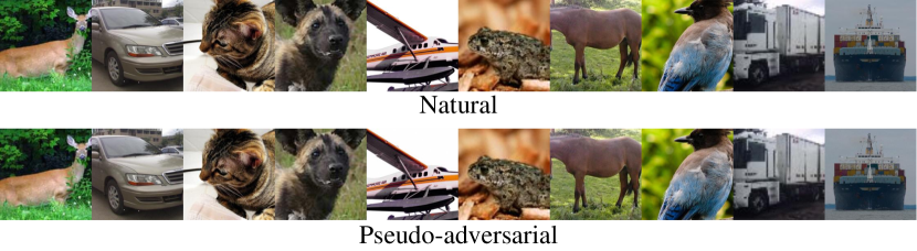
Figure 5: Natural images and corresponding pseudo-adversarial images generated by Perturbation Forgery.

References

- [1] Chen, J., Chen, H., Chen, K., Zhang, Y., Zou, Z., Shi, Z.: Diffusion models for imperceptible and transferable adversarial attack. arXiv preprint arXiv:2305.08192 (2023)
- [2] Chollet, F.: Xception: Deep learning with depthwise separable convolutions. In: 2017 IEEE Conference on Computer Vision and Pattern Recognition (CVPR). pp. 1800–1807 (2017). https://doi.org/10.1109/CVPR.2017.195
- [3] Deng, J., Dong, W., Socher, R., Li, L.J., Li, K., Fei-Fei, L.: Imagenet: A large-scale hierarchical image database. In: CVPR (2009)
- [4] Deng, J., Guo, J., Xue, N., Zafeiriou, S.: Arcface: Additive angular margin loss for deep face recognition. In: 2019 IEEE/CVF Conference on Computer Vision and Pattern Recognition (CVPR). pp. 4685–4694 (2019). https://doi.org/10.1109/CVPR.2019.00482
- [5] Deng, Z., Yang, X., Xu, S., Su, H., Zhu, J.: Libre: A practical bayesian approach to adversarial detection. In: Proceedings of the IEEE/CVF conference on computer vision and pattern recognition. pp. 972–982 (2021)
- [6] Dong, Y., Liao, F., Pang, T., Su, H., Zhu, J., Hu, X., Li, J.: Boosting adversarial attacks with momentum. In: CVPR. pp. 9185–9193 (2018)
- [7] Dong, Y., Pang, T., Su, H., Zhu, J.: Evading defenses to transferable adversarial examples by translation-invariant attacks. In: CVPR. pp. 4307–4316 (2019)
- [8] Du, X., Wang, Z., Cai, M., Li, Y.: Vos: Learning what you don’t know by virtual outlier synthesis. arXiv preprint arXiv:2202.01197 (2022)
- [9] Duda, R.O., Hart, P.E.: Pattern Classification and Scene Analysis. John Willey & Sons, New Yotk (1973)
- [10] Feinman, R., Curtin, R.R., Shintre, S., Gardner, A.B.: Detecting adversarial samples from artifacts. arXiv preprint arXiv:1703.00410 (2017)
- [11] Gary, B.H., Manu, R., Tamara, B., Erik, L.M.: Labeled faces in the wild: A database for studying face recognition in unconstrained environments. Technical Report 07-49, University of Massachusetts (2007)
- [12] Goodfellow, I.J., Shlens, J., Szegedy, C.: Explaining and harnessing adversarial examples (2014)
- [13] Gu, Q., Wang, G., Chiu, M.T., Tai, Y.W., Tang, C.K.: Ladn: Local adversarial disentangling network for facial makeup and de-makeup. In: 2019 IEEE/CVF International Conference on Computer Vision (ICCV). pp. 10480–10489 (2019). https://doi.org/10.1109/ICCV.2019.01058
- [14] He, K., Zhang, X., Ren, S., Sun, J.: Deep residual learning for image recognition. In: CVPR. pp. 770–778 (2016)
- [15] He, Y., Yu, N., Keuper, M., Fritz, M.: Beyond the spectrum: Detecting deepfakes via re-synthesis. In: Proceedings of the Thirtieth International Joint Conference on Artificial Intelligence, IJCAI-21. pp. 2534–2541. International Joint Conferences on Artificial Intelligence Organization (2021). https://doi.org/10.24963/ijcai.2021/349, https://doi.org/10.24963/ijcai.2021/349, main Track
- [16] Hu, S., Liu, X., Zhang, Y., Li, M., Zhang, L.Y., Jin, H., Wu, L.: Protecting facial privacy: Generating adversarial identity masks via style-robust makeup transfer. In: Proceedings of the IEEE/CVF Conference on Computer Vision and Pattern Recognition (CVPR). pp. 15014–15023 (2022)
- [17] Karras, T., Aila, T., Laine, S., Lehtinen, J.: Progressive growing of gans for improved quality, stability, and variation. arXiv preprint arXiv:1710.10196 (2017)
- [18] Kim, H.: Torchattacks: A pytorch repository for adversarial attacks. arXiv preprint arXiv:2010.01950 (2020)
- [19] Krizhevsky, A., Hinton, G., et al.: Learning multiple layers of features from tiny images. Technical report (2009)
- [20] Kurakin, A., Goodfellow, I., Bengio, S.: Adversarial machine learning at scale (2016)
- [21] Liang, S., Li, Y., Srikant, R.: Enhancing the reliability of out-of-distribution image detection in neural networks. arXiv preprint arXiv:1706.02690 (2017)
- [22] Lin, J., Song, C., He, K., Wang, L., Hopcroft, J.E.: Nesterov accelerated gradient and scale invariance for adversarial attacks. In: ICLR (2019)
- [23] Luo, Y., Zhang, Y., Yan, J., Liu, W.: Generalizing face forgery detection with high-frequency features. In: 2021 IEEE/CVF Conference on Computer Vision and Pattern Recognition (CVPR). pp. 16312–16321 (2021). https://doi.org/10.1109/CVPR46437.2021.01605
- [24] Ma, X., Li, B., Wang, Y., Erfani, S.M., Wijewickrema, S., Schoenebeck, G., Song, D., Houle, M.E., Bailey, J.: Characterizing adversarial subspaces using local intrinsic dimensionality (2018)
- [25] Madry, A., Makelov, A., Schmidt, L., Tsipras, D., Vladu, A.: Towards deep learning models resistant to adversarial attacks (2017)
- [26] Naseer, M.M., Khan, S.H., Khan, M.H., Shahbaz Khan, F., Porikli, F.: Cross-domain transferability of adversarial perturbations. Advances in Neural Information Processing Systems 32 (2019)
- [27] Naseer, M., Khan, S., Hayat, M., Khan, F.S., Porikli, F.: On generating transferable targeted perturbations. In: Proceedings of the IEEE/CVF International Conference on Computer Vision. pp. 7708–7717 (2021)
- [28] Ojha, U., Li, Y., Lee, Y.J.: Towards universal fake image detectors that generalize across generative models. In: Proceedings of the IEEE/CVF Conference on Computer Vision and Pattern Recognition. pp. 24480–24489 (2023)
- [29] Qin, X., Zhang, Z., Huang, C., Gao, C., Dehghan, M., Jagersand, M.: Basnet: Boundary-aware salient object detection. In: The IEEE Conference on Computer Vision and Pattern Recognition (CVPR) (June 2019)
- [30] Selvaraju, R.R., Cogswell, M., Das, A., Vedantam, R., Parikh, D., Batra, D.: Grad-cam: Visual explanations from deep networks via gradient-based localization. In: Proceedings of the IEEE international conference on computer vision. pp. 618–626 (2017)
- [31] Sharif, M., Bhagavatula, S., Bauer, L., Reiter, M.K.: Accessorize to a crime: Real and stealthy attacks on state-of-the-art face recognition. In: Proceedings of the 2016 acm sigsac conference on computer and communications security. pp. 1528–1540 (2016)
- [32] Shi, Y., Ling, H., Wu, L., Shen, J., Li, P.: Learning refined attribute-aligned network with attribute selection for person re-identification. Neurocomputing 402, 124–133 (2020). https://doi.org/https://doi.org/10.1016/j.neucom.2020.03.057, https://www.sciencedirect.com/science/article/pii/S0925231220304306
- [33] Tan, C., Zhao, Y., Wei, S., Gu, G., Wei, Y.: Learning on gradients: Generalized artifacts representation for gan-generated images detection. In: Proceedings of the IEEE/CVF Conference on Computer Vision and Pattern Recognition. pp. 12105–12114 (2023)
- [34] Tian, J., Zhou, J., Li, Y., Duan, J.: Detecting adversarial examples from sensitivity inconsistency of spatial-transform domain. In: Proceedings of the AAAI Conference on Artificial Intelligence. vol. 35, pp. 9877–9885 (2021)
- [35] Tong, L., Chen, Z., Ni, J., Cheng, W., Song, D., Chen, H., Vorobeychik, Y.: Facesec: A fine-grained robustness evaluation framework for face recognition systems. In: Proceedings of the IEEE/CVF Conference on Computer Vision and Pattern Recognition. pp. 13254–13263 (2021)
- [36] Tramèr, F., Kurakin, A., Papernot, N., Goodfellow, I., Boneh, D., McDaniel, P.: Ensemble adversarial training: Attacks and defenses. In: International Conference on Learning Representations (2018), https://openreview.net/forum?id=rkZvSe-RZ
- [37] Wang, Q., Xian, Y., Ling, H., Zhang, J., Lin, X., Li, P., Chen, J., Yu, N.: Detecting adversarial faces using only real face self-perturbations. In: IJCAI. pp. 1488–1496 (8 2023). https://doi.org/10.24963/ijcai.2023/165, https://doi.org/10.24963/ijcai.2023/165, main Track
- [38] Wang, S.Y., Wang, O., Zhang, R., Owens, A., Efros, A.A.: Cnn-generated images are surprisingly easy to spot… for now. In: Proceedings of the IEEE/CVF conference on computer vision and pattern recognition. pp. 8695–8704 (2020)
- [39] Wang, X., He, K.: Enhancing the transferability of adversarial attacks through variance tuning. In: CVPR. pp. 1924–1933 (2021)
- [40] Wang, Z., Bao, J., Zhou, W., Wang, W., Hu, H., Chen, H., Li, H.: Dire for diffusion-generated image detection. In: Proceedings of the IEEE/CVF International Conference on Computer Vision. pp. 22445–22455 (2023)
- [41] Wu, W., Su, Y., Lyu, M.R., King, I.: Improving the transferability of adversarial samples with adversarial transformations. In: CVPR. pp. 9020–9029 (2021)
- [42] Xue, H., Araujo, A., Hu, B., Chen, Y.: Diffusion-based adversarial sample generation for improved stealthiness and controllability. Advances in Neural Information Processing Systems 36 (2024)
- [43] Yang, X., Dong, Y., Pang, T., Su, H., Zhu, J., Chen, Y., Xue, H.: Towards face encryption by generating adversarial identity masks. In: ICCV. pp. 3877–3887 (2021)
- [44] Yin, B., Wang, W., Yao, T., Guo, J., Kong, Z., Ding, S., Li, J., Liu, C.: Adv-makeup: A new imperceptible and transferable attack on face recognition. In: Proceedings of the Thirtieth International Joint Conference on Artificial Intelligence, IJCAI-21. pp. 1252–1258. International Joint Conferences on Artificial Intelligence Organization (2021). https://doi.org/10.24963/ijcai.2021/173, https://doi.org/10.24963/ijcai.2021/173
- [45] Yoon, J., Hwang, S.J., Lee, J.: Adversarial purification with score-based generative models. In: ICML. pp. 12062–12072 (2021)
- [46] Zhang, H., Yu, Y., Jiao, J., Xing, E., El Ghaoui, L., Jordan, M.: Theoretically principled trade-off between robustness and accuracy. In: ICML. pp. 7472–7482 (2019)
- [47] Zhang, S., Liu, F., Yang, J., Yang, Y., Li, C., Han, B., Tan, M.: Detecting adversarial data by probing multiple perturbations using expected perturbation score. In: International Conference on Machine Learning. pp. 41429–41451. PMLR (2023)
- [48] Zhao, A., Chu, T., Liu, Y., Li, W., Li, J., Duan, L.: Minimizing maximum model discrepancy for transferable black-box targeted attacks. In: Proceedings of the IEEE/CVF Conference on Computer Vision and Pattern Recognition. pp. 8153–8162 (2023)