Deep Causal Generative Models with Property Control
Abstract
Generating data with properties of interest by external users while following the right causation among its intrinsic factors is important yet has not been well addressed jointly. This is due to the long-lasting challenge of jointly identifying key latent variables, their causal relations, and their correlation with properties of interest, as well as how to leverage their discoveries toward causally controlled data generation. To address these challenges, we propose a novel deep generative framework called the Correlation-aware Causal Variational Auto-encoder (C2VAE). This framework simultaneously recovers the correlation and causal relationships between properties using disentangled latent vectors. Specifically, causality is captured by learning the causal graph on latent variables through a structural causal model, while correlation is learned via a novel correlation pooling algorithm. Extensive experiments demonstrate C2VAE’s ability to accurately recover true causality and correlation, as well as its superiority in controllable data generation compared to baseline models.
1 Introduction
Significant advances have been achieved in the domain of learning low-dimensional representations and the generative mechanisms of complex, high-dimensional data, particularly in fields such as image synthesis Epstein et al. (2024); Wang et al. (2022), molecular design Xu et al. (2023); Born and Manica (2023), and natural language processing Zhang et al. (2023); Jin et al. (2024). Recently, research has shifted towards enhancing controlled generation, enabling the synthesis of data with specific properties by manipulating latent variables. Prominent examples include controlling facial expressions Klys et al. (2018), handwriting styles Kingma et al. (2014), and customizing object positions and sizes in images Guo et al. (2020). On another track, research interests have quickly increased in exploring the correlation and causality among latent variables, such as CausalVAE Yang et al. (2021), and DEAR Shen et al. (2022), which typically focus on the system’s intrinsic variables while ignoring their relations to the properties of interest of the practitioners. However, in practice, a more general and practical scenario is to generate the data causally while following the properties of interest, by exploring the unknown linkages between the properties and the latent variables. This underscores the need for a generative model capable of capturing both property correlations and their intrinsic causalities for controllable data generation (Figure 1 (a)). Moreover, understanding both correlation and causality could substantially avoid overcontrol and reduce the computational complexity during controllable generation processes. As illustrated in Figure 1 (b), rather than controlling all individual properties, which can be computationally intensive, optimizing a smaller set of root causes that influence all other causal variables and data properties might prove more efficient.
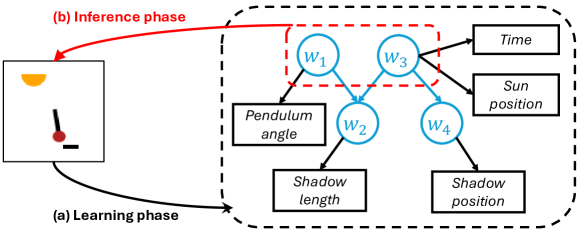
Despite the demand for deep generative models capable of controlling both property correlation and causality during data generation, challenges remain in: (1) Managing complex property relationships such as causality and correlation is difficult. Causality describes a direct cause-and-effect relationship between variables, exemplified by the change in shadow position and length due to the sun’s position, as shown in Figure 1. In contrast, correlation indicates a tendency for two variables to vary together, such as the sun’s position and time in the same figure. However, correlation does not necessarily indicate causality. While causality often leads to correlation, the relationship is directional and may sometimes even be unobservable; (2) Achieving model identifiability to simultaneously capture both property causality and correlation poses significant challenges. The latent representation of a model is identifiable when the model for learning the data is unique. However, the inherent complexity of data properties, uncovered by latent variables, and the intertwined causality and correlation between these properties, make identifying such a latent model challenging; (3) The succinctness of multi-objective optimization in controlling properties within the model is diminished when it does not account for their causal or correlated relationships. In data generation with controlled properties, multi-objective optimization typically involves each objective constraining one property. The complexity of multi-objective optimization grows rapidly in size with the number of objectives. However, for correlated or causal properties, optimizing one of them will also constrain the others into some subspace, leveraging causality or correlation between properties (e.g., Figure 1 (b)) to potentially reduce the number of objectives and ease the computational burden remains a significant yet under-explored approach.
To address the above challenges, we propose the Correlation-aware Causal Variational Autoencoder (C2VAE), a novel framework that recovers semantics, causality, and the correlation of properties via disentangled latent vectors. C2VAE incorporates an identifiable causal layer and a correlation layer to capture property causality and correlation. It also employs multi-objective optimization to control the properties of generated data, leveraging these causal and correlated relationships to streamline learning objectives and improve optimization efficiency. The contributions of this paper are summarized as follows:
-
•
A novel deep generative model for multi-objective control of causal and correlated properties. Beyond representation learning, we work on mapping specific target properties to latent variables, thus enhancing both interpretability and controllability. We introduce C2VAE, a novel framework designed for data generation with precise control over multiple properties. This identifiable model uncovers semantics, and causality as well as correlation of properties in latent variables via a causal layer and a correlation layer, respectively.
-
•
An efficient multi-objective optimization framework formulated for deep data generation. We introduce a novel multi-objective optimization framework that utilizes causality and correlation between properties to reduce the number of learning objectives, and therefore enhance optimization efficiency.
-
•
Extensive experiments are conducted to evaluate both generation quality and controllability of C2VAE. We conduct comprehensive experiments on three datasets to show the effectiveness of C2VAE. The results show that C2VAE can generate high-quality data and accurately control its properties.
2 Related works
2.1 Controllable Data Generation via Deep Learning
In the pursuit of controllable data generation through deep learning, the focus is on generating data using deep generative models while retaining specific properties (Wang et al., 2024). Although various deep generative models have emerged, existing methods can be classified into two scenarios based on the complexity of the relationships between the properties to be controlled: (1) independent property control and (2) causal and correlated property control. Controlling independent properties typically involves learning the dependencies between properties and latent variables while disentangling these latent variables to ensure their independence. For example, Locatello et al. (2019) developed SemiVAE, which factorizes the latent space and enforces each latent variable to be equal to the corresponding property value. Klys et al. (2018) designed CSVAE, where binary properties are captured by independent latent variables through adversarial learning. Furthermore, PCVAE proposed by Guo et al. (2020) extends CSVAE by enforcing an invertible mutual dependence between properties and latent variables, allowing control over the properties of generated data by manipulating the corresponding latent variables. By contrast, controlling correlated or even causal properties is a more complex task. Wang et al. (2022) extended PCVAE to CorrVAE by designing a mask pooling layer to capture property correlations using independent latent variables. The data can be generated by multi-objective optimization on latent variables. Yang et al. (2021) proposed CausalVAE, which controls causal properties by setting their values equal to latent variables and capturing their causality via a structural causal model (SCM). Shen et al. (2022) further improved CausalVAE with DEAR, which relaxes property supervision on latents through a learnable function that maps properties to latent variables. Given the complex property relationships in real-world data, controlling both property correlation and causality is crucial but remains under-explored, which motivates the development of our method.
2.2 Causal Representation Learning
Since causality often implies correlation—for example, altering the root cause typically changes the value of its effect—capturing causal property relationships in latent representation is inherently more complex than capturing mere correlations. Causal representation learning aims to uncover and represent the underlying causal structures within data. A common approach is to learn the causal graph using SCMs (Shimizu et al., 2006; Vowels et al., 2022), which was borrowed in both CausalVAE (Yang et al., 2021) and DEAR (Shen et al., 2022). Both works enforce the values of latent variables to match causal properties and capture these relationships using SCMs. In addition to SCMs, causal regularization (Bahadori et al., 2017) is a regularizer additive to the learning objective, weighted by the likelihood of edges of the causal graph to be learned. Besides, Rohekar et al. (2024) studied the relationship between self-attention and SCMs, finding that self-attention captures pairwise associations between symbols in an input sequence, which correspond exactly to those modeled by a linear-Gaussian SCM. However, those methods can recover causal relationships between variables, but cannot explicitly uncover their potential correlations. Therefore, we propose C2VAE that enables both causal and correlation discovery in the latent space of deep generative models.
3 Problem formulation
Given a dataset , in which each sample can be represented as with as properties of that can have correlation, casual relationship or be independent with each other. For instance, if the data is an image of the human face, properties can be gender, age, smile (whether the person smiles), beard (whether the person has a beard), etc. Here gender can be a cause of whether the person has a beard, and age and beard may have a correlation. We further assume that the data is generated via a certain random process from variables in a continuous latent space , where captures semantics of data properties and corresponds to all other concepts of data.
We aim to learn a generative model that generates conditioned on variables in and . Once the model is trained, users can generate data with target property values by editing the corresponding elements in . Combined with , this allows for the generation of new data with the desired properties. This goal raises the following question answered by our work: how to (1) jointly identify the latent variables in , the causal graph, and their relations to properties of interest; (2) generate data with true causes by controlling the properties.
4 Correlation-aware and Causal Variational Auto-encoder
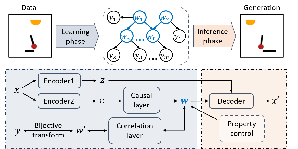
In this section, we delve into the details of the proposed C2VAE framework. Framework overview is shown in Figure 2. Specifically, C2VAE contains two phases: (1) Learning phase encodes properties of interest into latent variables, reconstructing their causal and correlated relationships in the latent space; (2) Inference phase generates data with desired property values while maintaining the correct correlation and causality with other properties.
The modeling of causal and correlated relationships requires the joint effort of different components, in addition to a basic VAE for disentangling concepts from data. C2VAE captures both causal and correlated relationships within properties through a causal layer and a correlation layer, respectively. During the learning phase, an input is first encoded into independent exogenous factors , which are further transformed into causal endogenous factors that correspond to causally related concepts in data through a learned causal graph. Afterward, a mask pooling layer is employed to uncover and analyze correlations between properties . This layer operates through carefully structured bridging latent variables . As a unified framework, C2VAE optimizes only the "root" latent variables (i.e., ) which hold all the causal and correlated relationships. During the inference phase, C2VAE enables the simultaneous manipulation of multiple properties through a multi-objective optimization approach. One can directly manipulate the root variables , which are combined with non-interested concepts (i.e., ) to generate data with the desired properties while maintaining the correct correlation and causality. The identifiability of the proposed C2VAE is discussed in Appendix A.
4.1 Learning phase
4.1.1 Overall learning objective based on probabilistic generative model
Based on the problem formulation in Section 3, the goal of C2VAE is not only to model the generation of from but also to model the dependence between and for controlling data properties. Therefore, we propose to achieve this goal by maximizing the joint log-likelihood via its evidence lower bound (ELBO):
| (1) |
The last equation in the above is based on the decomposition of into , and the following two assumptions: (1) and are conditionally independent given as only captures information from ; (2) is independent from and , which is equivalent to , as captures other concepts except data properties. Hence, the overall learning objective of C2VAE can be written as:
| (2) |
where , , and are the parameters of the decoder, property predictor (i.e., an MLP), and encoder, respectively. The last term of the objective function in Eq. 2 can be further decomposed into the following KL terms given that is independent of and :
| (3) |
where and are hyperparameters to penalize two terms. and are model parameters of the property encoder and the data encoder, respectively.
4.1.2 Causal Disentanglement Learning
Suppose there are concepts in data, to learn the causal representation of , we apply a causal layer that essentially describes a linear Structural Causal Model (SCM) (Shimizu et al., 2006). Note that might be smaller than the number of properties as some of them may share the same cause. Those concepts are causally structured by a Directed Acyclic Graph (DAG) with an adjacency matrix . Thereafter, the causal layer explicitly implements a linear SCM as follows:
| (4) |
where is the random noise of a causal model independent with , and is parameterized to be learned in the causal layer. As is the structured causal representation learned from the DAG, the matrix can be permuted into a strictly upper triangular matrix.
To address the identifiability issue of the learned causal graph mentioned in (Yang et al., 2021; Shen et al., 2022), we propose to supervise the conditional prior as follows:
| (5) |
where is a set of properties in that are correlated and controlled by ; is the total number of latent variables in . Furthermore, we assume the properties are continuous and follow a Gaussian distribution conditional on the corresponding latent variables in :
| (6) |
As it is trivial to have:
| (7) |
where is the Gaussian prior of . Therefore, the distribution of is still Gaussian and has two sufficient statistics . We will use this notation for indentifiability analysis in Appendix A.
4.1.3 Property Correlation-aware Conditional Prior
As we supposed, the correlation between properties is unknown, so (i.e., ) has to be learned by the model. To achieve this goal, we use a mask pooling layer , where is the dimension of the latent vector . captures how correlates with , where means correlates with the -th property ; otherwise, there is no correlation. In the meantime, to ensure the identifiability of , we mask all its upper triangular values. Thereafter, two variables that connect to the same variables in are regarded as correlated. The binary elements in are made trainable via the Gumbel Softmax function, while the norm of the mask matrix is added to the learning objective to encourage the sparsity of .
Given , we are able to collect the correlated properties (i.e., ) as follows:
| (8) |
Specifically, for properties , we can compute the corresponding that projects values from to each property as , where each column corresponds to the related latent variables in to predict the corresponding property in . Here, is a vector with all values set to one, and represents element-wise multiplication. For each property in , we aggregate all the information from its related latent variable set in into the next-level bridging variable via the aggregation function :
| (9) |
where is the parameter of the aggregation function . Finally, can be predicted using as:
| (10) |
where is the parameter of . The proposed framework aims to generate data that preserves the specific desired property values. Therefore it is natural to model the dependence between and (Wang et al., 2022), which encourages to propose an invertible function in Eq. 10 via a Lipschitz-constant constraint (Behrmann et al., 2019):
| (11) |
4.2 Inference phase
In this section, we introduce how to generate data given specific property values . The first step is to generate given . As we have learned an invertible mapping between and in Eq. 11, it is necessary to back-compute given by solving:
| (12) |
Next, given , we aim to infer . We naturally formalize this process of searching that satisfies specific property values as a multi-objective optimization framework. Note that we have:
| (13) |
given that is the bijective mapping from via an invertible function, the first term of Eq. 13 is the likelihood to predict , which can be modeled via Eq. 6. The second term is the prior distribution of , which is . Additionally, to reduce the complexity of the optimization process, we leverage the causal relationships between properties to minimize the number of variables to be optimized in . Specifically, we only use the root variables in the causal graph learned by Eq. 4, by masking other variables: , where is the vector of the -th column of . Therefore, the learning objective is formulated as:
| (14) |
The above optimization is achieved in a weighted-sum manner using general learning algorithms such as stochastic gradient descent or Adam. The learned is combined with sampled to serve as the input of the data decoder, which then generates the data.
5 Experiments
In this section, we present the experimental results and discuss our findings. The proposed method is compared against existing state-of-the-art methods for property-controllable generation and causal generation using three public datasets. We examine the quality of the generated data, the ability of each method to learn interpretable representations, and whether the outcomes of interventions on the learned latent variables align with our understanding of the correct correlation and causality.
5.1 Datasets
(1) Pendulum dataset was originally proposed to explore causality (Yang et al., 2021). It contains about 7k images featuring 3 entities (pendulum, light, shadow) and 4 properties (pendulum angle, light position) → (shadow position, shadow length). To introduce correlation, we add a property, time, which is correlated with light position. (2) Flow dataset was proposed to explore causality (Yang et al., 2021). It contains about 8k images featuring 4 properties (ball size → water height, (water height, hole) → water flow). A noise from was introduced to the gravitational acceleration. (3) dSprites dataset was originally proposed to explore disentanglement (Matthey et al., 2017). It contains about 730k images featuring 6 independent properties, from which we select scale, x position, and y position to construct 4 properties (scale, x position, x+y position, + position) to explore correlation and possible causality.
5.2 Comparison methods
(1) Semi-VAE pairs the latent variables with target properties by minimizing the MSE between latent variables and target properties (Kingma et al., 2014); (2) CSVAE correlates a subset of latent variables with properties by minimizing the mutual information (Klys et al., 2018); (3) PCVAE implements an invertible mapping between each pair of latent variables and properties by enforcing the mutual dependence (Guo et al., 2020). (4) CorrVAE uses a mask pooling layer to maintain the correlated mutual dependence between latent variables and properties (Wang et al., 2022). (4) CausalVAE learns causal representations of disentangled factors of data properties via a SCM (Yang et al., 2021). Additionally, we consider another method for ablation study. (5) C2VAE-true replaces the causal graph and correlation mask with ground-truth versions.
Method Pendulum Flow dSprites FID (↓) PSNR (↑) FID (↓) PSNR (↑) FID (↓) PSNR (↑) SemiVAE 33.83 14.96 28.79 23.96 74.47 12.08 CSVAE 40.26 14.97 29.05 23.97 51.01 12.13 PCVAE 28.17 14.93 29.69 24.07 95.94 12.19 CorrVAE 32.23 14.97 29.83 24.01 104.11 12.23 CausalVAE 31.04 19.38 11.10 26.12 166.97 22.56 C2VAE-true 10.60 23.33 5.51 28.78 109.82 19.73 C2VAE 25.81 19.72 8.81 26.56 95.24 21.53
Method Pendulum Flow dSprites MAE (↓) avgMI (↓) MAE (↓) avgMI (↓) MAE (↓) avgMI (↓) SemiVAE 0.23 0.81 0.25 0.59 2.97 1.60 CSVAE 8.99 1.55 12.16 1.00 7.57 1.04 PCVAE 0.34 0.80 0.28 0.58 3.24 1.59 CorrVAE 0.61 0.99 0.66 0.68 3.61 1.60 CausalVAE 0.48 1.05 1.32 0.97 2.73 0.98 C2VAE-true 0.65 1.02 0.44 0.79 2.66 0.78 C2VAE 0.18 0.79 0.19 0.56 2.43 0.83
5.3 Evaluation Metrics
For a comprehensive quantitative evaluation, we apply multiple metrics to measure data generation quality, property reconstruction accuracy, and the mutual dependence between latent variables and properties of interest. (1) Data generation quality: We use Frechet Inception Distance (FID) (Heusel et al., 2017) and Peak-Signal-to-Noise Ratio (PSNR) to assess the quality of generated images. FID compares the distribution of generated images with the distribution of a set of ground truth images. (2) Property reconstruction accuracy: We compute the Mean Absolute Error (MAE) between the model-predicted property values and their ground truth labels. (3) Mutual dependence: We use the average mutual information (avgMI) (Locatello et al., 2019), calculated as the Frobenius norm of the mutual information matrix of latent variables and properties and the ground-truth mask matrix. All experiments are conducted using an NVIDIA Tesla P100 GPU.
5.4 Insights from experimental results
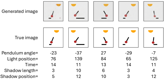
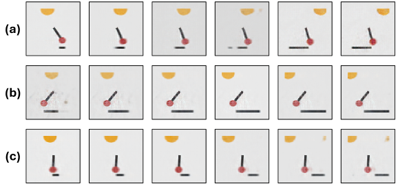
We evaluate the proposed C2VAE method by comparing it against other methods using three datasets according to (1) overall data generation quality, as shown in Table 1; (2) ability to identify correlation and causality between properties, depicted in Figure 3 and Figure 4; (3) control over property values, detailed in Table 2 and Figure 5; and (4) effectiveness of interventions on causal variables, illustrated in Figure 6. From the above experimental results, we can conclude that C2VAE demonstrates superior performance. Additionally, we have made several important observations based on these results.
C2VAE enhances performance on overall data generation quality. Despite being designed for controllable data generation via multi-objective optimization (Section 4.2), C2VAE maintains high-quality data generation. As shown in Table 1, C2VAE achieves an FID that is 7.30 (22.04) and 16.88 (65.71) lower on average than other methods on Pendulum and Flow, respectively. Additionally, its PSNR is 3.88 (24.48) and 2.13 (8.74) higher on average for these datasets. With the true causal graph and correlation mask, C2VAE-true outperforms all methods on both metrics. C2VAE does not outperform all methods on dSprites due to the inherent independence of its properties, which means that property learning is distinct from data generation. Combined with Table 2, it is evident that methods excelling in property-centered evaluations often generate lower-quality data on dSprites. For example, CSVAE achieves the best FID score but the worst MAE, indicating a trade-off between causal performance and data generation quality. Despite these challenges, among methods with constraints on property control or causal/correlation learning, C2VAE still maintains the best data generation quality.
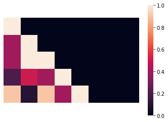
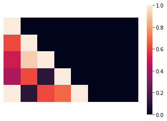
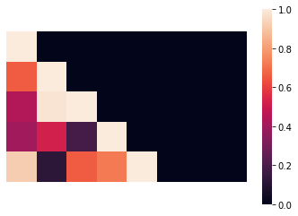
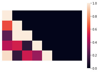
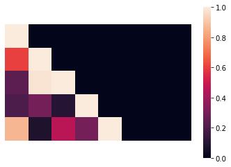
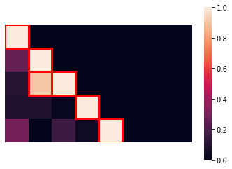
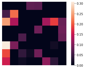
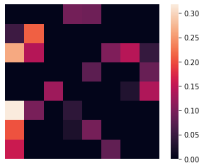
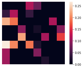
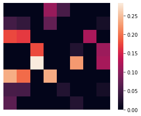
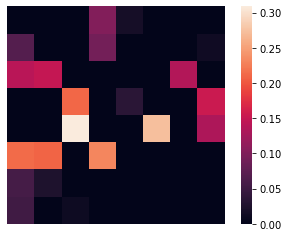

C2VAE uncovers correlation and causality between properties correctly. As shown in Figure 3, the correlation mask converges as the training epoch increases. Finally, controls both sun position and time, indicating that they are correlated, which is aligned with the truth. Besides, Figure 4 shows that the learned causal graph also converges along with the training process. The that controls time causes and to control shadow length and shadow position, respectively, which is also aligned with the truth.
C2VAE enables precise control over causal and correlated properties. Table 2 shows that C2VAE has superior performance regarding both MAE and avgMI compared with all other methods. Specifically, our C2VAE and its variant C2VAE-true consistently achieve the best MAE and avgMI on all three datasets, demonstrating superior performance in aligning latent variables with the properties. The MAE of C2VAE is 21.74% lower than the second-best method (SemiVAE) on Pendulum and 24.00% lower on Flow. While the improvement in the avgMI of C2VAE over SemiVAE is modest on Pendulum and Flow, it becomes substantial on dSprites, where the avgMI of C2VAE is almost half that of SemiVAE. Figures 5 and 6 demonstrate the controllable generation and intervention results, respectively. These results indicate that C2VAE achieves precise and accurate causal generation with effective property control.
6 Conclusion
In this paper, we explore the important problem of generating data with desired properties that maintain correlation and causality. We propose a novel framework named C2VAE, which recovers semantics, causality, and the correlation of properties via disentangled latent vectors. C2VAE incorporates an identifiable causal layer and a correlation layer to capture property causality and correlation. It controls properties of generated data via multi-objective optimization, leveraging these causal and correlated relationships to streamline learning objectives and improve optimization efficiency. Comprehensive experiments conducted on three public datasets demonstrate that C2VAE can generate high-quality data and accurately control properties. To the best of our knowledge, our work is the first to successfully implement deep causal generative models with property control, potentially paving the way for future advancements in generating data with reasoning capabilities.
Appendix A Identifiability Analysis
Suppose we model the encoder and the decoder in Eq. 2 via and , respectively. We define "identifiable" (Khemakhem et al., 2020) as follows:
Definition 1
Let be the binary relation on defined as follows: , and ,
where . If is an invertible matrix and is an invertible diagonal matrix with diagonal elements associated with properties, we say that the model parameter is identifiable.
We obtain the identifiability of our generative model as follows:
Theorem 1
Assume that we observe data sampled from a generative model parameterized by . The following holds:
-
1.
The set has the measure of zero, where is the characteristic function of the density .
-
2.
The funtion is differentiable and the Jacobian matrix of is of full rank.
-
3.
The sufficient statistics almost everywhere for all and , where is the statistic of variable .
-
4.
Properties satisfy that , i=1, 2, …, n.
Then parameters are identifiable.
The detailed proof is in Appendix B.
Appendix B Proof of Identifiability
Suppose we have two sets of parameters , such that for all data in . We want to prove . We have:
| (15) | ||||||
| (16) | ||||||
| (17) | ||||||
| (18) | ||||||
| (19) | ||||||
| (20) | ||||||
| (21) | ||||||
| (22) | ||||||
| (23) |
where:
| (24) |
As a result, we have the following equation:
| (25) |
Take the logarithm on both sides of Eq. 25, and replace by abstracting its expression in Eq. 7:
| (26) | |||
| (27) |
where is the base measure, is the normalization term, are the sufficient statistics and are the corresponding parameters depending on , and . is fixed and serves as the dimension of each sufficient statistic. We will have:
| (28) | |||
| (29) |
since for Gaussian distribution to index mean and variance. is in Gaussian distribution.
In the learning process, is constrained as DAG, so that exists and is full-rank. To enforce the equality of Eq. 29, terms that are not related to are cancelled out:
| (30) |
where is a vector related to .
To model the SCM, we have , and is modeled by . In addition, Hence, the equation above becomes:
| (31) |
Let be a diagonal matrix as:
| (32) |
Assume , is full-rank. Plug in Eq. 30, which becomes:
| (33) |
where:
| (34) |
Replace with then we have:
| (35) | |||
| (36) |
where . Note that since is invertible and is invertible. According to Lemma 3 in Khemakhem et al. (2020), we can choose a pair such that are linearly independent. Then, concatenate the two points into a vector and denote the Jacobian matrix and define on in the same way. By differentiating Eq. 36, we have:
| (37) |
Since is of full-rank, so that and are both invertible. Based on Eq. 37, is invertible. In the same way, similarly, we can prove is invertible. As a result, is identifiable.
References
- Bahadori et al. [2017] Mohammad Taha Bahadori, Krzysztof Chalupka, Edward Choi, Robert Chen, Walter F Stewart, and Jimeng Sun. Causal regularization. arXiv preprint arXiv:1702.02604, 2017.
- Behrmann et al. [2019] Jens Behrmann, Will Grathwohl, Ricky TQ Chen, David Duvenaud, and Jörn-Henrik Jacobsen. Invertible residual networks. In International conference on machine learning, pages 573–582. PMLR, 2019.
- Born and Manica [2023] Jannis Born and Matteo Manica. Regression transformer enables concurrent sequence regression and generation for molecular language modelling. Nature Machine Intelligence, 5(4):432–444, 2023.
- Epstein et al. [2024] Dave Epstein, Allan Jabri, Ben Poole, Alexei Efros, and Aleksander Holynski. Diffusion self-guidance for controllable image generation. Advances in Neural Information Processing Systems, 36, 2024.
- Guo et al. [2020] Xiaojie Guo, Yuanqi Du, and Liang Zhao. Property controllable variational autoencoder via invertible mutual dependence. In International Conference on Learning Representations, 2020.
- Heusel et al. [2017] Martin Heusel, Hubert Ramsauer, Thomas Unterthiner, Bernhard Nessler, and Sepp Hochreiter. Gans trained by a two time-scale update rule converge to a local nash equilibrium. Advances in neural information processing systems, 30, 2017.
- Jin et al. [2024] Wei Jin, Haitao Mao, Zheng Li, Haoming Jiang, Chen Luo, Hongzhi Wen, Haoyu Han, Hanqing Lu, Zhengyang Wang, Ruirui Li, et al. Amazon-m2: A multilingual multi-locale shopping session dataset for recommendation and text generation. Advances in Neural Information Processing Systems, 36, 2024.
- Khemakhem et al. [2020] Ilyes Khemakhem, Diederik Kingma, Ricardo Monti, and Aapo Hyvarinen. Variational autoencoders and nonlinear ica: A unifying framework. In International Conference on Artificial Intelligence and Statistics, pages 2207–2217. PMLR, 2020.
- Kingma et al. [2014] Durk P Kingma, Shakir Mohamed, Danilo Jimenez Rezende, and Max Welling. Semi-supervised learning with deep generative models. Advances in neural information processing systems, 27, 2014.
- Klys et al. [2018] Jack Klys, Jake Snell, and Richard Zemel. Learning latent subspaces in variational autoencoders. Advances in neural information processing systems, 31, 2018.
- Locatello et al. [2019] Francesco Locatello, Michael Tschannen, Stefan Bauer, Gunnar Rätsch, Bernhard Schölkopf, and Olivier Bachem. Disentangling factors of variation using few labels. arXiv preprint arXiv:1905.01258, 2019.
- Matthey et al. [2017] Loic Matthey, Irina Higgins, Demis Hassabis, and Alexander Lerchner. dsprites: Disentanglement testing sprites dataset. https://github.com/deepmind/dsprites-dataset/, 2017.
- Rohekar et al. [2024] Raanan Y Rohekar, Yaniv Gurwicz, and Shami Nisimov. Causal interpretation of self-attention in pre-trained transformers. Advances in Neural Information Processing Systems, 36, 2024.
- Shen et al. [2022] Xinwei Shen, Furui Liu, Hanze Dong, Qing Lian, Zhitang Chen, and Tong Zhang. Weakly supervised disentangled generative causal representation learning. Journal of Machine Learning Research, 23(241):1–55, 2022.
- Shimizu et al. [2006] Shohei Shimizu, Patrik O Hoyer, Aapo Hyvärinen, Antti Kerminen, and Michael Jordan. A linear non-gaussian acyclic model for causal discovery. Journal of Machine Learning Research, 7(10), 2006.
- Vowels et al. [2022] Matthew J Vowels, Necati Cihan Camgoz, and Richard Bowden. D’ya like dags? a survey on structure learning and causal discovery. ACM Computing Surveys, 55(4):1–36, 2022.
- Wang et al. [2022] Shiyu Wang, Xiaojie Guo, Xuanyang Lin, Bo Pan, Yuanqi Du, Yinkai Wang, Yanfang Ye, Ashley Petersen, Austin Leitgeb, Saleh AlKhalifa, et al. Multi-objective deep data generation with correlated property control. Advances in Neural Information Processing Systems, 35:28889–28901, 2022.
- Wang et al. [2024] Shiyu Wang, Yuanqi Du, Xiaojie Guo, Bo Pan, Zhaohui Qin, and Liang Zhao. Controllable data generation by deep learning: A review. ACM Computing Surveys, 56(9):1–38, 2024.
- Xu et al. [2023] Minkai Xu, Alexander S Powers, Ron O Dror, Stefano Ermon, and Jure Leskovec. Geometric latent diffusion models for 3d molecule generation. In International Conference on Machine Learning, pages 38592–38610. PMLR, 2023.
- Yang et al. [2021] Mengyue Yang, Furui Liu, Zhitang Chen, Xinwei Shen, Jianye Hao, and Jun Wang. Causalvae: Disentangled representation learning via neural structural causal models. In Proceedings of the IEEE/CVF conference on computer vision and pattern recognition, pages 9593–9602, 2021.
- Zhang et al. [2023] Hanqing Zhang, Haolin Song, Shaoyu Li, Ming Zhou, and Dawei Song. A survey of controllable text generation using transformer-based pre-trained language models. ACM Computing Surveys, 56(3):1–37, 2023.