Pin the loop taut: a one-player topologame

Abstract

We introduce a $1$-player game called pin the loop and analyse its complexity. A loop is a generic immersion of the circle in a surface, considered up to isotopy. A loop is taut when it is minimally intersecting in its homotopy class. A pinning set of a loop is a set of points $P$ in the surface avoiding the loop, such that the loop is taut in the surface punctured at $P$. The pinning number is the minimal cardinal of its pinning sets, and a pinning set is optimal if it has that cardinal.

We show that the decision problem associated to computing the pinning number of a plane loop is NP-complete. We implement a polynomial algorithm to check if a given point-set is pinning, adapting a method of Birman–Series for computing intersection numbers of curves in surfaces. After improving a theorem of Hass–Scott characterising taut loops in surfaces, we reduce the problem to a boolean formula whose solutions correspond to the pinning sets. Finally, we reduce the vertex-cover problem for graphs to an instance of the pinning problem for plane loops.

Our results imply that given a closed geodesic in a complete Riemannian surface with punctures, it is hard to guess the location of the punctures from the sole isotopy class of the geodesic in the compactified surface.

Figure 1: A loop with $2$ optimal pinning sets, and $3$ other minimal pinning sets. Created with SnapPy [CDGW].

0 Introduction

Multiloops and their pinning semi-lattices

Let $\mathbb{F}$ be a closed oriented smooth surface (we will often focus on the case of a sphere, which already contains most of the intricacies). For a finite set of points $P\subset\mathbb{F}$ we write $\mathbb{F}_{P}=\mathbb{F}\setminus P$. Denote by $\sqcup_{1}^{s}\mathbb{S}$ a disjoint union of $s\in\mathbb{N}$ oriented circles.

A multiloop with $s$ strands is a generic immersion $\gamma\colon\sqcup_{1}^{s}\mathbb{S}\looparrowright\mathbb{F}_{P}$ considered up to orientation preserving diffeomorphisms of the source and the target. Here generic means that all multiple points are transverse double-points.

A multiloop $\gamma$ yields a $4$-valent embedded graph $\Gamma\hookrightarrow\mathbb{F}_{P}$ where $\Gamma=\operatorname{im}(\gamma)$. The regions of $\gamma$ or $\Gamma$ are the connected components of $\mathbb{F}\setminus\Gamma$, indexed by $R=\pi_{0}(\mathbb{F}\setminus\Gamma)$. A multiloop is called filling when its regions are homotopic to discs, which is always satisfied when $\mathbb{F}$ is a sphere: we will abreviate it as multifiloop.

A multicurve is a homotopy class of multiloops. The set of multicurves is endowed with the self-intersection function $\operatorname{si}(\gamma)$ counting the minimal number of double-points among its generic representatives. A multiloop is taut when it has the minimal number of double-points in its homotopy class.

Definition 0.1 (pinning set).

Consider a multiloop $\gamma\colon\sqcup_{1}^{s}\mathbb{S}\looparrowright\mathbb{F}$ with regions $R$. We say that a set of regions $P\subset R$ is a pinning set if puncturing the surface $\mathbb{F}$ in those regions yields a taut multiloop $\gamma\colon\sqcup_{1}^{s}\mathbb{S}\looparrowright\mathbb{F}_{P}$. The pinning sets of $\gamma$ form its pinning semi-lattice: a subposet $\mathcal{L}\subset\operatorname{\mathcal{P}}(R)$ closed under union and containing $R$.

A pinning set is called minimal if it is minimal with respect to inclusion, and optimal if it has the minimum cardinal among all pinning sets. The pinning number $\varpi(\gamma)\in\mathbb{N}$ is the cardinal of its optimal pinning sets.

Remark 0.2 (motivation).

It follows from [NC01] that a multiloop is taut if and only if it is isotopic to a union of shortest geodesics for some Riemannian metric. In that sense, the taut multiloops are those which have a physical meaning.

Hence given a multiloop in $\mathbb{F}$, one may wonder where must there have been punctures to have it realised as a geodesic?

Question 0.3 (goal).

Given a multiloop $\gamma\colon\sqcup_{1}^{s}\mathbb{S}\looparrowright\mathbb{F}$, how (efficiently) can we:

• Construct minimal or optimal pinning sets?

• Find which regions belong to every pinning set?

• Compute the pinning number $\varpi(\gamma)$?

More generally we wonder what can be the shape of the pinning semi-lattice of a (multi)loop, and what are its statistics for certain random models.

We will address all of these questions, with a particular emphasis on the following.

Theorem 0.4 (MultiLooPiNum).

The MultiLooPiNum problem defined by

• A filling multiloop $\gamma\colon\sqcup_{1}^{s}\mathbb{S}\looparrowright\mathbb{F}$, and an integer $p\in\mathbb{N}$.

• Does $\gamma$ have pinning number $\varpi(\gamma)\leq p$?

is strongly NP-complete, so as its restriction to loops in the sphere $\gamma\colon\mathbb{S}\looparrowright\mathbb{S}^{2}$.

0.1 Combinatorial group theory: counting self-intersections

A filling multiloop $\gamma\colon\sqcup_{1}^{s}\mathbb{S}\looparrowright\mathbb{F}$ is determined, modulo orientation of its strands, by its associated $4$-valent filling graph $\Gamma\subset\mathbb{F}$, which can be encoded by a pair of permutations over its set of half-edges. We will use the size $\lvert\gamma\rvert$ of such an encoding as a measure of complexity: it is proportional to $\operatorname{Card}(R)+\lvert\chi(\mathbb{F})\rvert$.

Algorithm 0.5 (self-intersection).

We will describe an algorithm which has:

• A plane multiloop $\gamma\colon\sqcup_{1}^{s}\mathbb{S}\looparrowright\mathbb{F}$ together with a subset of regions $P\subset R$.

• The self-intersection number of the multicurve $\gamma\colon\sqcup_{1}^{s}\mathbb{S}\looparrowright\mathbb{F}_{P}$.

• Running time $O(\lvert\gamma\rvert^{2})$.

The algorithm first computes a convenient presentation of the free group $\pi_{1}(\mathbb{F}_{R})$. Its generators correspond to the edges of a spanning tree of the dual graph of $\Gamma\subset\mathbb{F}$. The homotopy classes of the loops $\gamma_{i}\subset\mathbb{F}_{R}$ correspond to conjugacy classes in that free group, whence to cyclically reduced words in the generators. Filling the regions $Q=R\setminus P$ yields explicit relations providing a presentation of $\pi_{1}(\mathbb{F}_{P})$, and we deduce the conjugacy classes associated to $\gamma_{i}\subset\mathbb{F}_{P}$ by applying simple rewriting rules. Finally we adapt an algorithm of Birman–Series and Cohen–Lustig to compute the intersection number between homotopy classes.

Corollary 0.6 (Pinning and PinMin are P).

Given a plane multiloop $\gamma$ and a subset of regions $P\subset R$, we can successively:

• certify that $P$ is pinning in time $O(\lvert\gamma\rvert^{2})$, and if so

• check if $P$ is a minimal pinning set in time $O(\operatorname{Card}(P)\lvert\gamma\rvert^{2})$, and if not

• construct a minimal pinning set $M\subset P$ in time $O(\operatorname{Card}(P)\lvert\gamma\rvert^{2})$.

Remark 0.7 (higher genus).

We will present the algorithm 0.5 for loops in the sphere but it can be adapted to any genus without essential modifications.

The Corollary 0.6 holds identically in that context.

Corollary 0.8 (MultiLooPiNum is NP).

The MultiLooPiNum problem is in NP.

0.2 Geometric topology: computing immersed discs

This subsection focuses on filoops, namely multifiloops with one strand, and the corresponding LooPiNum problem.

We already know from Corollary 0.8 that it is in NP, but we will provide an explicit reduction to a certain boolean equation, which reveals the structure of the problem and will also help us to show that it is strongly NP-hard.

For this we will need to improve [HS85, Theorem 4.2]. The statement relies on the Definitions 2.3 and 2.7 of an immersed monorbigon for a loop $\gamma$, which are subloops delimited by one or two double-points that bound an immersed disc.

Theorem 0.9 (taut loops have no immersed monorbigons).

Consider a closed oriented surface $\mathbb{F}$ together with a set of points $P\subset\mathbb{F}$, and a loop $\gamma\colon\mathbb{S}\looparrowright\mathbb{F}_{P}$.

The loop $\gamma\looparrowright\mathbb{F}_{P}$ is not taut if and only if it has an immersed monorbigon.

Algorithm 0.10 (pinning mobidiscs).

Given a filoop $\gamma\colon\mathbb{S}\to\mathbb{F}$ with regions $R$, we will construct in time $O(\operatorname{Card}(R)^{2}\operatorname{Card}(V)^{2})$ a collection $\operatorname{MoB}(\gamma)\subset\operatorname{\mathcal{P}}(R)$ with the property that $P\in\operatorname{\mathcal{P}}(R)$ is pinning if and only if it intersects every $D\in\operatorname{MoB}(\gamma)$.

The algorithm 0.10 implies that the pinning sets of the loop $\gamma$ correspond to the solutions of the monotone conjunctive normal form associated to $\operatorname{MoB}(\gamma)\subset\operatorname{\mathcal{P}}(R)$, or equivalently to the vertex-covers of the hyper-graph whose vertices are indexed by the regions $R$ and hyper-edges correspond to the mobidiscs $\operatorname{MoB}(\gamma)\subset\operatorname{\mathcal{P}}(R)$. Finding the minimum cardinal for these solutions is known to be in NP, and we will explain how it may be solved efficiently with a particular type of SAT-solver.

Corollary 0.11.

The LooPiNum problem is in NP.

The Theorem 0.9 will also serve to justify the validity of the following reduction.

Algorithm 0.12 (reduction from planar vertex cover to LooPinNum).

We describe a polynomial time algorithm which to a planar graph $G=(V,E)$ associates a plane loop $\gamma\colon\mathbb{S}\to\mathbb{R}^{2}$ with $O(\operatorname{Card}(E)^{2})$ double-points, such that the $k$-vertex-covers of $G$ are in one to one correspondence with the $(k+2\operatorname{Card}(E)$)-pinning-sets of $\gamma$.

Note that the LooPiNum problem contains that same problem for loops in the sphere, so its complexity is at least as hard as the planar vertex cover problem, which is known to be strongly NP-complete [GJ78][§3 para. 7].

Corollary 0.13.

The LooPiNum problem is strongly NP-hard, even in the sphere.

0.3 The pinning semi-lattice of a multiloop

Consider a multiloop $\gamma\colon\sqcup_{1}^{s}\mathbb{S}\looparrowright\mathbb{F}$ with regions $R$. Its pinning semi-lattice $\mathcal{L}\subset\operatorname{\mathcal{P}}(R)$ carries much more information related to the pinning problem for the multiloop.

Using Algorithm 0.5 and some functionalities from plantri [BM], we computed the pinning semi-lattices of all irreducible indecomposible spherical multiloops with at most $14$ regions (unoriented and up to reflection), and the statistics of certain numerical parameters. The results are available as a data base at this link.

We make a few observations in section 3, either suggesting certain heuristics for approximation algorithms, or invalidating some naïve conjectures about the behaviour of pinning-semi lattices. Let us record the main questions and observations.

Question 0.14 (structure of pinning semi-lattices).

Which join semi-lattices arise as pinning semi-lattices of filling loops or multiloops?

How do pinning semi-lattices of multifiloops behave under Reidemeister moves, flypes, and crossing resolutions?

How do pinning semi-lattices of loops behave under the operations of spheric-sums and toric-sums introduced in [Sim23]?

The Figures 18 and 19 show that the pinning number can change under $R3$ moves and flypes as well as mutations, even for indecomposible loops in the sphere.

Figure 2: A multiloop and the part of its pinning semi-lattice obtained by taking unions of minimal pinning sets (in red or green), together with the set of all regions.

0.4 Further directions of research and related works

Multiloops versus loops.

The validity of Algorithm 0.10, reducing LooPiNum to the vertex cover problem for hypergraphs, relies on results which hold for loops but sometimes fail for multiloops with $\geq 2$ strands.

Question 0.15 (loops versus multiloops).

Does the MultiLooPiNum problem belong to a strictly larger complexity class than LooPiNum? This would be a finer complexity distinction since the present work shows that both are strongly NP-complete.

By Algorithm 0.10, the pinning semi-lattice of a loop $\gamma$ with regions $R$ is isomorphic to the solution semi-lattice of the monotone conjunctive normal form associated to $\operatorname{MoB}(\gamma)\subset\operatorname{\mathcal{P}}(R)$. The pinning semi-lattice of multiloops is more mysterious.

Question 0.16 (counting strands).

Can one find a topological notion generalising mobidiscs to multiloops, which would yield a basis for the pinning semi-lattice ?

Can we compute or estimate lower bounds for the number of strands of a multiloop from its pinning semi-lattice?

Question 0.17 (multi-simple-loops).

We may restrict the MultiLooPinNum to multi-simple-loops $\gamma\colon\sqcup_{1}^{s}\mathbb{S}^{1}\looparrowright\mathbb{F}$, namely whose double points involve distinct strands.

It can be approached using methods similar to those in subsection 2.2, relying on [FM12, Proposition 1.7]. Indeed, one may show that the problem is in P if we restrict to $s\leq 3$ strands, and NP-complete if we do not restrict $s\in\mathbb{N}$. Is there a critical value of $s\in\mathbb{N}$ for which it is NP-complete?

Approximate solutions and heuristics.

When facing an NP-complete problem, one wonders whether it is possible to find approximate solutions in polynomial time.

Question 0.18 (approximability).

Does there exist $\epsilon_{1},\epsilon_{2}>0$ and a polynomial time algorithm which given a multiloop $\gamma$ and $k\in\mathbb{N}$ either confirms that $\varpi(\gamma)>k$ or else constructs $P\subset R$ with $\operatorname{Card}P\leq(1+\epsilon_{1})k$ and $\operatorname{si}(\gamma,P)>(1-\epsilon_{2}).\operatorname{si}(\gamma,R)$?

A weaker expectation would be an algorithm based on certain heuristics which computes an approximate solution with high probability (that is on most entries).

Question 0.19 (heuristics).

Are there heuristics building on the idea of pinning regions of small degree and certain embedded monorbigons which lead to algorithms that find approximate solutions with high probability? We discuss some in section 3.

Geometric algorithms.

Given a multiloop $\gamma\colon\sqcup_{1}^{s}\mathbb{S}\looparrowright\mathbb{F}$ and a subset of regions $P\subset R$ such that $\chi(\mathbb{F}_{P})<0$, one could apply geometric algorithms to check whether $P$ is pinning, by applying a curve shortening flow [HS94, DL19].

For instance, choose a negatively curved metric on $\mathbb{F}_{P}$ and apply a geometric curve-shortening flow algorithm relying on gradient descent: the multiloop $\gamma\colon\mathbb{S}\looparrowright\mathbb{F}_{P}$ is not taut if and only if it develops a self-tangency or a cusp under this flow.

Pinning statistics for random multiloops.

Consider a random model for unoriented multiloop in closed orientable surfaces (in fixed genus or not), by choosing a distribution on a set of $4$-valent maps, each one being weighted proportionally to the inverse cardinal of its automorphism group. What is the distribution of:

• the size of an optimal pinning set, that is the pinning number?

• the number of optimal pinning sets, and of minimal pinning sets?

Other variational problems.

Fix a filling multiloop $\gamma\colon\sqcup_{1}^{s}\mathbb{S}\looparrowright\mathbb{F}$, we may consider several increasing functionals on its poset of regions $R$: to a set $P\in R$ we can associate its cardinal $\operatorname{Card}(P)=\sum_{P_{i}\in P}1$, its total degree $\deg(P)=\sum_{P_{i}\in P}\deg(P_{i})$, and minus the self-intersection number $-\operatorname{si}(\gamma,P)$ of the multicurve $\gamma\colon\sqcup_{1}^{s}\mathbb{S}\looparrowright\mathbb{F}_{P}$.

The pinning problems addressed in this work concern the local and global minima $P\in R$ of the functional $\operatorname{Card}(P)$ in restriction to the level-set $\{P\in R\mid\operatorname{si}(\gamma,P)=n\}$ where $n$ is the number of double-points of the multiloop $\gamma$.

If we change $\operatorname{Card}(P)$ for $\deg(P)$, then we may apply Algorithm 0.5 to deduce an analogous Corollary 0.6 showing that certain pinning problems are in P.

Moreover, we believe that the $\deg$-weighted analog LooPinDeg of the LooPinNum problem is also strongly-NP-complete. By adapting Algorithm 0.12, can one reduce the problem of finding a vertex cover for a planar graph with minimal total vertex degree to the desired LooPinDeg problem?

Question 0.20.

There are other interesting functionals to extremize, which from a game theoretic perspective can be thought as varying the cost or gain function, and that may yield other interesting topological invariants of multifiloops.

What is the complexity of computing the minimal values of the monotonous functionals $\operatorname{Card}(P)-\operatorname{si}(\gamma,P)$ or $\deg(P)-\operatorname{si}(\gamma,P)$? What about non-monotonous functionals of the form $4\operatorname{Card}(P)-\deg(P)-3\operatorname{si}(\gamma,P)$? ()

Which monotonous functions depending on $(\operatorname{Card}(P),\deg(P))$ and $-\operatorname{si}_{P}(\gamma)$ have global minimal values that are in P to compute? What are the topological interpretations of these quantities?

Pinning invariants for homeomophisms.

Let $\psi\in\operatorname{Homeo}_{0}(\mathbb{F})$ be a homeomorphism which is isotopic to the identity.

For a multiloop $\gamma\colon\sqcup\mathbb{S}\looparrowright\mathbb{F}$, we may define the minimum among the representatives in its isotopy class of the pinning number $\varpi(\gamma\cup\psi(\gamma))$, and compare it with $\varpi(\gamma)+\varpi(\psi(\gamma))=2\varpi(\gamma)$. One may think of this quantity as measuring the minimum number of points at which one must place punctures in $P\subset\mathbb{F}$ to obtain a topological model for the action of a class $[\psi]\in\operatorname{Map}(\mathbb{F}_{P})$ on $\gamma\subset\mathbb{F}_{P}$. Now, for a certain class of multiloops $\mathcal{C}$ (say all multiloops, or multiloops with no double points), we define

$$\varpi(\psi,\mathcal{C})=\min\{\varpi(\psi,\gamma)\mid\gamma\in\mathcal{C}\}.$$

The case where $\mathcal{C}$ are a loops with no double points appears closely related to the work [BHW22] about quasi-morphisms on the groups $\operatorname{Homeo}_{0}(\mathbb{F})$ and $\operatorname{Diff}_{0}(\mathbb{F})$. Indeed, their main tool is to relate the action of $\psi\in\operatorname{Diff}_{0}(\mathbb{F})$ on the fine curve graph of $\mathbb{F}$ to the actions of $[\psi]\in\operatorname{Map}(\mathbb{F}_{P})$ on the surviving curve graphs of $\mathbb{F}_{P}$. We believe that the quantities $\varpi(\psi,\mathcal{C})$ may be of interest for such investigations.

Complexity of link invariants.

The fact that MultiLooPiNum and LooPiNum are NP-complete follows a general trend of complexity results regarding the computation of numerical invariants in topology.

Many numerical invariants in topology are NP-hard to decide, such as for instance the Betti numbers of cell complexes [SL23].

More closely related to the present work, the genus of a knot [AHT02], the unlinking number of a knot [KT21], the crossing number of a knot [dMSS20], and all so-called intermediate invariants of knots and links [dMRST21] have been shown to be NP-hard to decide. The problem of unknot recognition is noteworthy in that it belongs to $\texttt{NP}\cap\texttt{co-NP}$ [HLP99, Lac21].

As mentioned in [dMRST21], upper bounds on the complexity of deciding numerical invariants of knots and links are often elusive. In contrast, the present work shows that certain subtle measures of the complexity of multiloops are more tractable.

Other games.

There are countless variations of the one-player game pin the loop, including two-player versions in the style of Nim. We hope to explore some of these in forthcoming work.

1 Combinatorial group theory: counting self-intersections

In the first subsection we encode multifiloops $\gamma\colon\sqcup\mathbb{S}\looparrowright\mathbb{F}$ by $4$-valent maps. We used it extensively in our own implementations of our algorithms, but it can be safely skipped without any hindrance to understanding the mathematical content of this work.

In the second subsection we use this to derive a presentation of the fundamental group $\pi_{1}(\mathbb{F}_{P})$ together with the conjugacy classes associated to the strands of $\gamma$.

In the third subsection we explain an algorithm to compute the self-intersection number of the multicurve associated to $\gamma$ in $\mathbb{F}_{P}$.

Altogether they imply Corollary 1.10, saying certain pinning problems are in P.

1.1 Encoding filling multiloops as $4$-valent maps

Let us first explain well known encoding for filling graphs and filling multiloops. A general reference for this is [LZ04].

A map $\Gamma\subset\mathbb{F}$ is an embedded graph in our closed oriented surface whose complement is a disjoint union of discs, considered up to orientation preserving diffeomorphisms.

Lemma 1.1.

A map $\Gamma\subset\mathbb{F}$ with $n$ edges corresponds to a pair of permutations $\epsilon,\sigma\in\mathfrak{S}_{2n}$ considered up to conjugacy, such that:

• $\epsilon$ has orbits of size $2$ corresponding to the edges

• $\sigma$ has orbits corresponding to the vertices

• $\varphi=(\sigma\epsilon)^{-1}$ has orbits corresponding to the regions

The degree of a vertex or region is the cardinal of the corresponding orbit for $\sigma$ or $\varphi$. The Euler characteristic of $\mathbb{F}$ is the alternated sum of the number of orbits of $\sigma,\epsilon,\varphi$. The dual map of $\Gamma\subset\mathbb{F}$ is obtained by exchanging $\sigma$ and $\varphi$.

Remark 1.2.

For a map $\epsilon,\sigma\in\mathfrak{S}_{2n}$ and a union of orbits of $\varphi=(\epsilon\sigma)^{-1}$, the corresponding union of closed regions and its interior have homotopy types which may be computed in polynomial time on $n$. For example, we often wish to determine their number of connected components and their genera.

A filling multiloop $\gamma\colon\sqcup_{1}^{s}\mathbb{S}\looparrowright\mathbb{F}$ is determined, modulo orientation of its strands, by its associated $4$-valent map $\Gamma\subset\mathbb{F}$. Note that the orientation of $\gamma$ corresponds to an orientation of the edges of $\Gamma$ which go straight on at each vertex.

Lemma 1.3.

A $4$-valent map $\Gamma\subset\mathbb{F}$ with $n$ edges corresponds to a pair of permutations $\epsilon,\sigma\in\mathfrak{S}_{2n}$ considered up to conjugacy, such that:

• $\epsilon$ has orbits of size $2$ corresponding to the edges

• $\sigma$ has orbits of size $4$ corresponding to the vertices

• $\varphi=(\sigma\epsilon)^{-1}$ has orbits corresponding to the regions

Moreover, the orbits of $\delta=\epsilon\sigma^{2}$ define the oriented strands of $\Gamma$, and these are paired by $\epsilon$ to form its unoriented strands. If a multiloop $\gamma$ yields the map $\Gamma$, the oriented strands of $\gamma$ select one orbit of $\delta$ in each $\epsilon$-pair.

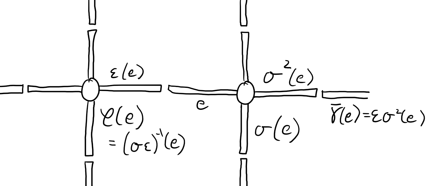
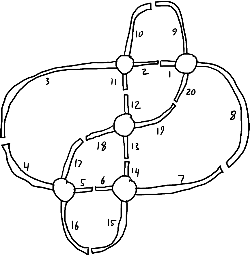
Figure 3: A map with labelled half-edges. The permutations $\epsilon,\sigma,\varphi,\delta$. Right:

$$\begin{split}\epsilon&=(1,2)(3,4)(5,6)(7,8)(9,10)(11,12)(13,14)(15,16)(17,18)(19,20),\\ \sigma&=(8,9,1,20)(2,10,3,11)(5,17,4,16)(7,14,6,15)(19,12,18,13),\\ \varphi&=(1,11,19)(2,9)(3,17,12)(4,10,8,15)(5,14,18)(6,16)(7,20,13),\\ \delta&=(1,7,5,3)(2,4,6,8)(9,19,17,15,13,11)(10,12,14,16,18,20).\end{split}$$

The following observation will serve only to find (multi)loops in the sphere whose regions all have degree $\geq 3$ with the minimal number of regions.

Lemma 1.4.

For a $4$-valent map $\Gamma\subset\mathbb{F}$ in a surface of Euler characteristic $\chi$, the degree of the regions $R_{i}\in R$ satisfying

$$\textstyle\sum_{R_{i}\in R}(\deg(R_{i})-4)=-4\chi.$$

In particular, a multiloop in the torus has average region-degree $4$, and a multiloop in the sphere whose regions have degree $\geq 3$ has at least $8$ regions of degree $3$.

Proof.

Denote the vertices by $V$, the edges by $E$ and the regions by $R$. The $4$-valency of the graph implies that $2\rvert E\rvert=4\lvert V\rvert$. The surface embedding yields $\sum_{R}\deg R_{i}=2\lvert E\rvert=4\lvert V\rvert$. The filling property computes the Euler characteristic $\chi=\lvert V\rvert-\lvert E\rvert+\lvert R\rvert$ so that $\lvert R\rvert=\chi+\lvert V\rvert$. Combine these, we find that for all $m\in\mathbb{N}$ we have $\sum_{R}(\deg(R_{i})-m)=(4-m)\lvert V\rvert-m\chi$, whence $\sum_{R}(\deg R_{i}-4)=-4\chi$. ∎

Figure 4: All irreducible indecomposible spherical multiloops with at most $12$ regions and all region-degrees $\geq 3$ (unoriented and up to reflection; see [OEI24, A078666]), with regions labelled by their degrees. Generated with plantri [BM] and drawn with SnapPy [CDGW].

1.2 From multiloops to words in the free group

In this subsection we restrict, for simplicity of the exposition, to the case $\mathbb{F}=\mathbb{S}^{2}$.

Consider a multiloop $\gamma\colon\sqcup_{1}^{s}\mathbb{S}\looparrowright\mathbb{F}$ together with a set of regions $P\subset R$. We address the question of checking whether $P$ is a pinning-set, namely whether $\gamma$ is a taut loop in the surface $\mathbb{F}_{P}=\mathbb{F}\setminus P$.

The multiloops $\gamma$ admitting a pinning-set of cardinal $\leq 1$ are those with no double-points. From now on we assume that $p-1=\operatorname{Card}(P)>0$.

We choose a base point $\infty\in\mathbb{F}\setminus\Gamma$ in a region belonging to $P$, called the unbounded region. Hence the fundamental group $\pi_{1}(\mathbb{F}_{P},\infty)$ is free of rank $p$.

Remark 1.5 ($\varpi(\gamma)=2$).

A loop $\gamma$ with $\varpi(\gamma)=2$ is a “snail”, that is a generic perturbation of the $n$-th power of a circle which has $n-1$ double-points. The multiloops $\gamma$ with $\varpi(\gamma)=2$ are the disjoint unions of circles and at least one concentric snail.

Recall that a multiloop $\gamma\colon\sqcup_{1}^{s}\mathbb{S}\looparrowright\mathbb{F}$ is determined, modulo orientation of its strands, by its associated $4$-valent plane graph $\Gamma\subset\mathbb{F}$. In its dual graph $\Gamma^{*}\subset\mathbb{F}$, we choose to include $\infty$ as a vertex which we call the root.

Fix a spanning tree $T^{*}$ for the dual graph $\Gamma^{*}\subset\mathbb{F}$, orient its edges outwards from the root vertex $\infty$, and co-orient them using the orientation of the disc. We also order its vertices and its edges by a depth first search from $\infty$.

Step 1: $\pi_{1}(\mathbb{F}_{R},\infty)$.

We first compute an explicit presentation for the free group $\pi_{1}(\mathbb{F}_{R},\infty)$ where $R=\pi_{0}(\mathbb{F}\setminus\Gamma)$ consists of all regions, from which we may easily express the conjugacy classes of the strands $\gamma_{j}$. The construction follows Figure 5.

Consider simple loops $\tau_{1},\dots,\tau_{r}$ which intersect only at their base point $\infty$, such that $\tau_{j}$ intersects $T^{*}$ only at the edge with label $r$ and in the direction prescribed by its co-orientation. The free group $\pi_{1}(\mathbb{F}_{R},\infty)$ is freely generated by $\tau=\{\tau_{1},\dots,\tau_{r}\}$. The symmetric generating set $\tau^{\pm}=\{\tau_{j}^{\pm 1}\mid 1\leq j\leq r\}$ inherits the cyclic order given by the emergence of paths from $\infty$. The complement $\mathbb{F}\setminus T^{*}$ is a polygon whose $2r$ edges are labelled by $\tau^{\pm}$ in accordance with its cyclic order. It lifts in the universal cover of $\mathbb{F}_{R}$ to a fundamental domain under the action of $\pi_{1}(\mathbb{F}_{R},\infty)$, whose generators $\tau^{\pm}$ identify its edges two-by-two.

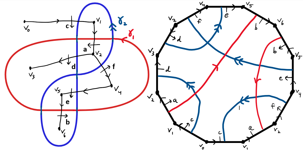
Figure 5: A multiloop, a dual tree, and its polygonal domain in the universal cover. Left image created with SnapPy [CDGW].

Note that each strand $\gamma_{j}$ of $\gamma$ corresponds to a conjugacy class in $\pi_{1}(\mathbb{F}_{R},\infty)$, hence to a unique reduced cyclic word over $\tau^{\pm}$ which may be computed by recording the sequence of edges of $T^{*}$ that it crosses, minding the co-orientation to determine the exponent of each generator.

Step 2: $\pi_{1}(\mathbb{F}_{P},\infty)$.

Now for a subset of regions $P\subset R$, we deduce a presentation of the free group $\pi_{1}(\mathbb{F}_{P},\infty)$, and the new reduced cyclic words associated to the conjugacy classes of the strands $\gamma_{j}$. The construction follows Figure 6.

By the van Kampen Theorem, the group $\pi_{1}(\mathbb{F}_{P},\infty)$ is the quotient of $\pi_{1}(\mathbb{F}_{R},\infty)$ by the normal subgroup generated by small loops only surrounding the punctures to be filled, associated to the set of regions $Q=R\setminus P$.

A region $R_{j}\in R$ corresponds to a non-rooted vertex of $T^{*}$, which has one incoming edge and a certain number of outgoing edges. Let $\rho_{j}$ be the word over $\tau^{\pm}$ obtained by reading the cutting sequence of $T^{*}$ of a loop winding once around $R_{j}$, starting at the incoming edge. Thus $\rho_{j}$ is a product of $\deg(R_{j})$ generators in $\tau^{\pm}$ which are all distinct even up to inversion. We deduce the presentation:

$$\pi_{1}(\mathbb{F}_{P},\infty)=\pi_{1}(\mathbb{F}_{R},\infty)\mod{\vartriangleleft\{\rho_{j}\mid R_{j}\in Q\}\vartriangleright}$$

in which every relator $\rho(R_{j})$ yields a rewriting rule of the form $\tau_{j_{1}}\mapsto\tau^{\mp}_{j_{d}}\cdots\tau^{\mp}_{j_{2}}$ which we obtain by solving the equation $\rho(R_{j})=\mathfrak{1}$.

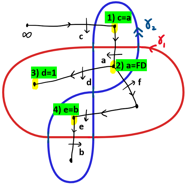
$$\gamma_{1}:ab\mapsto_{2}FDb\mapsto_{3}Fb.\quad\gamma_{2}:cdef\mapsto_{1}adef\mapsto_{2}FDdef\mapsto Fef\mapsto_{4}Fbf\mapsto b.$$

Figure 6: Filling punctures, adding relations, and applying rewriting rules in DFS order. Created with SnapPy [CDGW].

Moreover, for an arbitrary word $\alpha$ over $\tau^{\pm}$, we may apply these rewriting rules in the order prescribed by a depth first search from $\infty$ to obtain a canonical representative of $\alpha$ in $\pi_{1}(\mathbb{F}_{P},\infty)$ which uses none of the generators associated to regions in $Q$. This holds in particular for the words associated to the strands of $\gamma$.

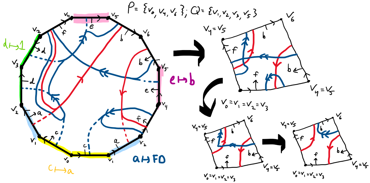
Figure 7: The fundamental domain of $\mathbb{F}_{R}$ collapses to that of $\mathbb{F}_{P}$. The pairs of edges identified by $\tau_{j}$ for $R_{j}\in Q$ get collapsed to ideal points.

Observe that the remaining generators $\tau^{\pm}_{P}=\{\tau_{j}^{\pm}\mid R_{j}\in P\}$ of $\pi_{1}(\mathbb{F}_{P},\infty)$ inherit a cyclic order from $\tau^{\pm}$, which is compatible with their action on a lift of $\mathbb{F}_{P}\setminus T^{*}$ to a polygonal fundamental domain in the universal cover of $\mathbb{F}_{P}$. See Figure 7.

1.3 Computing self-intersection of homotopy classes

In this subsection we adapt an algorithm proposed in [CL87] extending [BS84, BS87] and [Rei62] to compute the self-intersection number of a multicurve $\gamma$ in $\mathbb{F}_{P}$.

The algorithm we propose takes as input a free group $\mathcal{F}_{p}$ of rank $p$ over a set $\tau=\{\tau_{j}\mid 1\leq j\leq p\}$ with a cyclic order on the symmetric set $\tau^{\pm}$, and a finite set $\gamma$ of reduced cyclic words in these generators. It returns the self-intersection number:

$$\textstyle\operatorname{si}(\gamma)=\sum_{k}\operatorname{si}(\gamma_{k})+\sum_{i\neq j}\operatorname{i}(\gamma_{i},\gamma_{j})$$

Remark 1.6.

For curves $\alpha,\beta$ in $\mathbb{F}_{P}$ and $a,b\in\mathbb{N}$ we have $\operatorname{i}(\alpha^{a},\beta^{b})=ab\cdot\operatorname{i}(\alpha,\beta)$. Note that the self-intersection number of a curve satisfies $\operatorname{si}(\alpha)=\tfrac{1}{2}\operatorname{i}(\alpha,\alpha)$.

If $\alpha$ is primitive then for all $n\in\mathbb{N}^{*}$ we have $\operatorname{si}(\alpha^{n})=n^{2}\operatorname{si}(\alpha)+(n-1)$. Conversely, if there exists $n\in\mathbb{N}_{>1}$ such that $\operatorname{si}(\alpha^{n})=n^{2}\operatorname{si}(\alpha)+(n-1)$ then $\alpha$ is primitive (because otherwise $\alpha=\beta^{m}$ for some primitive $\beta$ and $m\in\mathbb{N}_{>1}$, and applying the previous formula to $\alpha^{n}=\beta^{mn}$ would lead to $m\leq 1$, a contradiction).

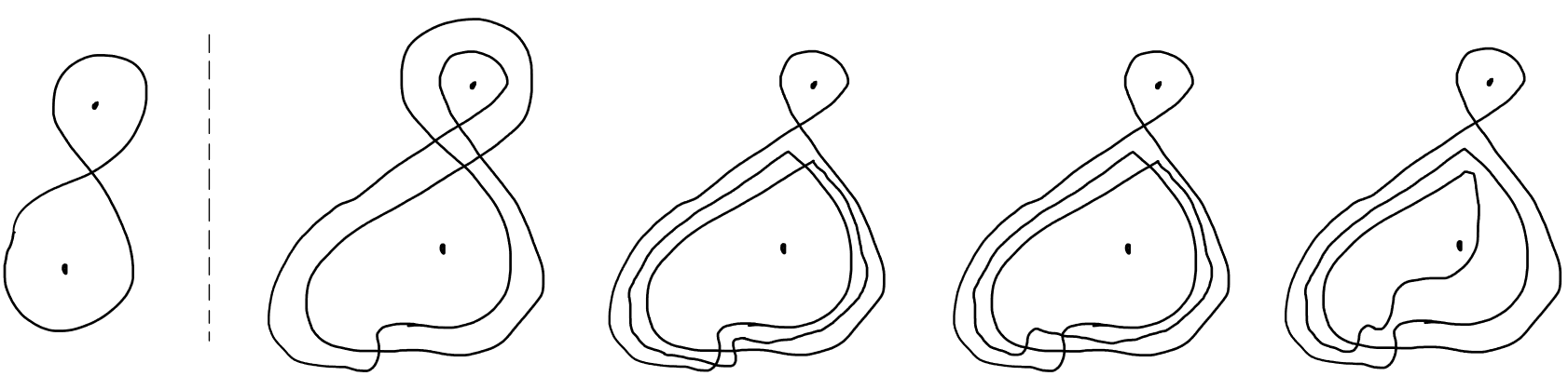
Figure 8: The primitivity assumption on $\alpha$ is important to compute $\operatorname{si}(\alpha^{n})=n^{2}\operatorname{si}(\alpha)+(n-1)$. With $\alpha$ as the figure eight in the twice punctured sphere (left), one finds a sequence of moves (right) showing $\operatorname{si}(\alpha^{2})=3$. This does not contradict the formula as $\alpha$ is in fact not primitive. Adding an additional puncture at infinity makes $\alpha$ primitive, whence we find $\operatorname{si}(\alpha^{2})=5$ as predicted by the formula.

The Cayley graph of $(\mathcal{F}_{p},\tau^{\pm})$ is the infinite $2p$-regular tree $\mathcal{T}_{p}$ with a base vertex $\mathfrak{1}$, whose edges around each vertex are labelled by $\tau^{\pm}$. The cyclic order on $\tau^{\pm}$ yields a planar embedding of $\mathcal{T}_{p}$, and extends to a cyclic order $\operatorname{cord}(x,y,z)$ on the boundary $\partial\mathcal{T}_{p}$, which we identify with the subset $(\tau^{\pm})^{\mathbb{N}}$ of reduced one sided sequences. This yields an intersection function $\operatorname{cross}(\alpha,\beta)\in\{0,\pm 1/2,\pm 1\}$ on its set of complete geodesics, which we identify with the subset $(\tau^{\pm})^{\mathbb{Z}}$ of reduced two sided sequences:

$$\operatorname{cross}(\alpha,\beta)=\tfrac{1}{2}\left(\operatorname{cord}(\alpha_{+},\beta_{+},\alpha_{-})-\operatorname{cord}(\alpha_{+},\beta_{-},\alpha_{-})\right)$$

We define the order of contact $\operatorname{val}(\alpha,\beta)\in\mathbb{Z}$ between two oriented geodesics as their number of common vertices in $\mathcal{T}_{p}$, with sign comparing the orientations of the axes along their intersection. Observe that $\operatorname{val}(\alpha,\beta)=0\implies\operatorname{cross}(\alpha,\beta)=0$.

An element $\alpha\in\mathcal{F}_{p}\setminus\{\mathfrak{1}\}$ acts by translation of $\mathcal{T}_{p}$ along an axis joining its endpoints $\alpha_{-},\alpha_{+}\in\partial\mathcal{T}_{p}$. When $\alpha\in\mathcal{F}_{p}$ is cyclically reduced, its axis passes through the base vertex $\mathfrak{1}\in\mathcal{T}_{p}$, and is labelled by the periodisation $\alpha^{\infty}\in(\tau^{\pm})^{\mathbb{Z}}$. The conjugacy classes of $\mathcal{F}_{p}$ correspond to reduced cycles of words on $\tau^{\pm}$.

The periodisation map $\mathcal{F}_{p}\setminus\{\mathfrak{1}\}\to(\tau^{\pm})^{\mathbb{Z}}$ denoted $\alpha\mapsto\alpha^{\infty}$ is injective in restriction to cyclically reduced primitive words. Denote by $\sigma$ the Bernoulli shift on the subset of reduced words in $(\tau^{\pm})^{\mathbb{Z}}$ which moves all letters to the left, as well as the cyclic shift on cyclically reduced words of $\mathcal{F}_{p}\setminus\{\mathfrak{1}\}$ which moves the first letter at the end. These shifts are intertwined by the periodisation map: $(\sigma^{j}\alpha)^{\infty}=\sigma^{j}(\alpha^{\infty})$.

Proposition 1.7 (Intersection).

For conjugacy classes represented by cyclically reduced words $\alpha,\beta\in\mathcal{F}_{p}\setminus\{\mathfrak{1}\}$, their intersection number is given by:

$$\operatorname{i}(\alpha,\beta)=\sum_{i=1}^{\operatorname{len}(\alpha)}\sum_{j=1}^{\operatorname{len}(\beta)}\left|\frac{\operatorname{cross}(\sigma^{i}\alpha,\sigma^{j}\beta)}{\operatorname{val}(\sigma^{i}\alpha,\sigma^{j}\beta)}\right|$$

counting the pairs of cyclically reduced representatives of the conjugacy classes up to simultaneous conjugacy, whose endpoints are linked.

1.4 The complexity of the algorithm and its consequences

Algorithm 1.8 (self-intersection).

We have described an algorithm which has:

• A plane multiloop $\gamma\colon\sqcup_{1}^{s}\mathbb{S}\looparrowright\mathbb{F}$ together with a subset of regions $P\subset R$.

• The self-intersection number of the multicurve $\gamma\colon\sqcup_{1}^{s}\mathbb{S}\looparrowright\mathbb{F}_{P}$.

• Running time $O(\lvert\gamma\rvert^{2})$.

Proof.

Consider a plane multiloop $\gamma$ of size $\lvert\gamma\rvert$ with a subset of regions $P\subset R$.

We begin by choosing any tree spanning the dual graph of $\Gamma$, deriving a presentation of the free group $\mathbb{F}_{P}$, and computing the reduced cyclic words associated to the homotopy classes of the strands $\gamma_{j}$. All this can be done in time $O(\lvert\gamma\rvert)$.

Then we computed the self-intersection number of the multiloop. For this we must factor the cyclic words as powers of their primitive roots, in a time which is at most quadratic in the length of the word. Then we run the computations of the form $\operatorname{si}(\alpha,\beta)$ in a time proportional to the product of the word lengths of $\alpha$ and $\beta$. By the Cauchy Schwartz inequality, the time to compute $\operatorname{si}(\gamma)$ is in $O(\lvert\gamma\rvert^{2})$.

Let us note that the running time for $\operatorname{i}(\alpha,\beta)$ relies on the following observation. For any finite words $u,v$ we have $u^{\infty}=v^{\infty}\iff uv=vu$, which means that for words in the free group $\mathcal{F}_{p}$ over an ordered set of generators $x_{0},\dots,x_{p}$, we may compute the cyclic order $\operatorname{cross}(u,v)$ in time $O(\operatorname{len}(u)+\operatorname{len}(v))$. ∎

Remark 1.9 (higher genus).

This algorithm adapts to compute the intersection number between two loops in any oriented surface $\mathbb{F}$ with a free fundamental group.

For this one must choose a base point $\infty\in\mathbb{F}$ which is (close to) a puncture, and perform cuts along disjoint simple arcs between the punctures to represent $\mathbb{F}$ as the identification of the sides of a $2n$-gon whose vertices are removed.

This yields a presentation for $\pi_{1}(\mathbb{F}\setminus\{\infty\})=\mathcal{F}_{n}$ by a free set of generators, together with a cyclic order on the corresponding symmetric generating set.

The complexity is still $O(\lvert\gamma\rvert^{2})$, keeping in mind that since $\gamma$ is filling we have $\lvert\gamma\rvert=\operatorname{Card}(R)+\lvert\chi(\mathbb{F})\rvert$.

Corollary 1.10 (Pinning and PinMin are P).

Given a plane multiloop $\gamma$ and a subset of regions $P\subset R$, we can successively:

• certify that $P$ is pinning in time $O(\lvert\gamma\rvert^{2})$, and if so

• check if $P$ is a minimal pinning set in time $O(\operatorname{Card}(P)\lvert\gamma\rvert^{2})$, and if not

• construct a minimal pinning set $M\subset P$ in time $O(\operatorname{Card}(P)\lvert\gamma\rvert^{2})$.

Proof.

Consider a multiloop $\gamma\colon\sqcup_{1}^{s}\mathbb{S}\to\mathbb{F}$ and a set of regions $P\subset R$. We may compute the self-intersection number of the multicurve $\gamma\subset\mathbb{F}_{P}$ using the previous algorithm in time $O(\lvert\gamma\rvert^{2})$, and compare it with the number of double-points of $\gamma$. This checks whether $P$ is pinning, and if so confirms that $\varpi(\gamma)\leq\operatorname{Card}(P)$, proving the NP complexity of MultiLooPinNum.

Now suppose that we have checked that $P$ is pinning. To a linear order of $P$ we associate a minimal pinning subset computed as follows. We construct a decreasing chain of pinning sets, starting with $P$, by trying to remove them one by one.

We try removing the first region and check if the new set is pinning in time $O(\lvert\gamma\rvert^{2})$: if it is we continue with that new set, otherwise we move to the next region. By doing so, we never need to try removing a pin twice: either it was already removed, or we know it cannot be removed. Thus in the worst case we need to call at most $\operatorname{Card}(P)$ times to our $O(\lvert\gamma\rvert^{2})$ checking algorithm.

Note that this construction defines a surjective function from the set of linear orders of $R$ to the set of minimal pinning sets of $\gamma$. ∎

Corollary 1.11 (MultiLooPiNum is NP).

The MultiLooPiNum problem, defined by

• A filling multiloop $\gamma\colon\sqcup_{1}^{s}\mathbb{S}\looparrowright\mathbb{F}$, and an integer $p\in\mathbb{N}$.

• Does $\gamma$ have pinning number $\varpi(\gamma)\leq p$?

belongs to the class NP.

2 Geometric topology: computing immersed discs

This section focuses on filoops, namely multifiloops with one strand.

The first subsection recalls how they correspond to framed chord diagrams.

The second subsection will put their pinning sets in correspondence with the satisfying assignments of a positive conjunctive normal form (which we define). In particular the pinning number and an optimal pinning set of a filoop can be found using a certain type of SAT-solver, and the corresponding problems are in NP.

The third subsection will reduce the vertex cover problem for planar graphs to our LoopPinNum problem, proving it is Strongly NP-hard (for any genus).

2.1 Encoding filling loops with chord diagrams

Let us recall from [Car91] how filoops correspond to framed chord diagrams.

Fix a loop $\gamma\colon\mathbb{S}\looparrowright\mathbb{F}$ with $m$ self-intersections. Each intersection $x\in\gamma(\mathbb{S})$ has two preimages $x_{\infty},x_{0}\in\mathbb{S}$ ordered so that $(\vec{\gamma}(x_{\infty}),\vec{\gamma}(x_{0}))$ forms a positive basis of the tangent plane $T_{x}\mathbb{F}$.

This yields a framed chord diagram of size $m$, namely a cyclic word $C$ on the the set of $2m$ framed-letters $\{x_{0}(1),x_{\infty}(1),\dots,x_{0}(m),x_{\infty}(m)\}$ considered up to relabelling of the $m$ letters $\{x(1),\dots,x(m)\}$.

Observe that inverting the orientation of the source $\mathbb{S}$ of $\gamma$ corresponds to inverting the cycle $C$, whereas inverting the orientation of the target $\mathbb{F}$ of $\gamma$ corresponds to exchanging all values of $\{0,\infty\}$ of the framing.

Lemma 2.1 (filling loops = framed chord diagrams).

Every framed chord diagram arises from a unique filling loop.

The conversions between framed chord diagrams and $4$-valent maps is of linear time complexity in the number of edges.

Proof.

To a framed chord diagram $C$ of size $m$ letters we associate a $4$-valent map $\Gamma\subset\mathbb{F}$ with $2m$ edges encoded by a pair of permuations $\sigma,\delta\in\mathfrak{S}_{4m}$ as in Lemma 3.

Each letter $x$ corresponds to a vertex incident to $4$ half-edges $x_{\infty}^{+},x_{0}^{+},x_{\infty}^{-},x_{0}^{-}$ in that cyclic order: these are the $m$ orbits of $\sigma$. These half-edges are connected in the cyclic order prescribed by the cycle $C$ after duplicating each framed-letter as $x_{o}\rightsquigarrow x_{o}^{-}x_{o}^{+}$: these are the $2$ orbits of $\delta$.

We may thus construct a ribbon-graph as in Figure 9, and attach discs to its boundary components to obtain a filling map $\Gamma\subset\mathbb{F}$. The cycle $C$ selects one of the two Eulerian circuits of $\Gamma$ which are transverse at every vertex. This yields a filling loop $\gamma$, whose associated framed chord diagram is the one we started with.

Figure 9: Constructing the ribbon-graph associated to a framed chord diagram

∎

Remark 2.2 (Regions and genus of $C$).

If $C$ has chords $V$ and $\gamma$ has regions $R$, then $\mathbb{F}$ has Euler characteristic $2-2g=\operatorname{Card}(R)-\operatorname{Card}(V)$.

The regions of $\gamma$ can be read off $C$ by travelling along the circle, jumping across each chord that is met along the way, and pursuing along the circle in the same or opposite direction according to the framing.

Figure 10: Reading the regions of $\gamma$, for example on $C=a_{\infty}c_{0}d_{\infty}b_{0}c_{\infty}a_{0}d_{\infty}b_{0}$.

2.2 Taut loops, their monorbigons and mobidiscs

In this subsection we fix an oriented surface $\mathbb{F}$ with a set of points $P\subset\mathbb{F}$. Consider a loop $\gamma\colon\mathbb{S}\looparrowright\mathbb{F}_{P}$ which may be filling or not, giving rise to a framed chord diagram $C$ with chords labelled by $V$.

Definition 2.3 (singular monorbigons).

A singular monogon is a non-trivial closed interval $I\subset C$ such that $\gamma(\partial I)=\{x\}$ for some $x\in V$ and $\gamma(I)$ is null-homotopic. This singular monogon is embedded when $\gamma$ is injective on the interior of $I$.

A singular bigon is a disjoint union of non-trivial closed intervals $I\sqcup J\subset C$ such that $\gamma(\partial I)=\{x,y\}=\gamma(\partial J)$ for some $x,y\in V$ and $\gamma(I\sqcup J)\subset\mathbb{F}$ is null-homotopic. This singular bigon is embedded when $\gamma$ is injective on the interior of $I\sqcup J$.

A singular monorbigon $K$ refers to a singular monogon $I$ or singular bigon $I\sqcup J$. The restriction $\gamma(K)$ is a subloop of $\gamma$ and we call $\gamma(\partial K)$ its marked points.

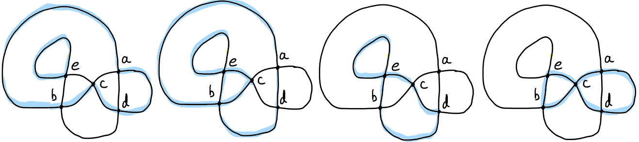
Figure 11: Examples of singular monorbigons: embedded, and non-embedded.

Remark 2.4 (homology).

A singular monorbigon $K=I$ or $K=I\sqcup J$ yields a subloop $\alpha=\gamma(K)$ which is homotopically trivial in $\mathbb{F}_{P}$, hence trivial in homology.

In particular $\alpha$ is trivial in $H_{1}(\mathbb{F}_{P};\mathbb{Z}/2)$ so it is two-sided. Moreover $\alpha$ is trivial in $H_{1}(\mathbb{F}_{P};\mathbb{Z})$, so for every pair of points $p_{0},p_{1}\in P$ we have that $\operatorname{wind}(\alpha;p_{0},p_{1})=0$.

Algorithm 2.5 (computing singular monorbigons).

For a filoop $\gamma\colon\mathbb{S}\looparrowright\mathbb{F}$ and a subset of regions $P\subset R$, we can list all singular monorbigons of $\gamma\colon\mathbb{S}\looparrowright\mathbb{F}_{P}$ in time $O(\operatorname{Card}(V)^{2}\times\operatorname{Card}(R))$.

Proof.

First list the $2\operatorname{Card}(V)$ intervals $I$ and $<2\operatorname{Card}(V)^{2}$ interval unions $I\sqcup J$ satisfying the conditions in definition 2.3, except the homotopical triviality.

Then, check if the subloop $\gamma(I)$ or $\gamma(I\sqcup J)$ is homotopically trivial by computing the associated word in the fundamental group $\pi_{1}(\mathbb{F}_{P})$ as in subsection 1.2. ∎

Our interest in the concept of embedded and singular monorbigons lies in the following Theorems which were proven by Hass-Scott in [HS85].

Theorem 2.6 (taut loops have no singular monorbigons).

Consider a closed oriented surface $\mathbb{F}$ together with a set of points $P\subset\mathbb{F}$, and a loop $\gamma\colon\mathbb{S}\looparrowright\mathbb{F}_{P}$.

Recall that $\operatorname{si}(\gamma)$ denotes the self-intersection number of its homotopy class in $\mathbb{F}_{P}$.

• If $\gamma$ has $>0$ double-points but $\operatorname{si}(\gamma)=0$, then $\gamma$ has an embedded monorbigon.

• If $\gamma$ has $>\operatorname{si}(\gamma)$ double-points, then it has a singular monorbigon.

For the purpose of pinning loops, we will need to improve these results.

Definition 2.7 (immersed monorbigons and mobidiscs).

Consider a loop $\gamma\colon\mathbb{S}\to\mathbb{F}_{P}$ with $K\subset\mathbb{S}$ singular monorbigon $K=I$ or $K=I\sqcup J$.

We say that $K$ is an immersed monorbigon when there exists an immersion $\iota\colon\mathbb{D}\looparrowright\mathbb{F}_{P}$ such that the restriction $\gamma\colon K\looparrowright\mathbb{F}_{P}$ factors through $\iota\colon\partial\mathbb{D}\looparrowright\mathbb{F}_{P}$.

A mobidisc consists of the regions of $\gamma$ in the image $\iota(\mathbb{D})$ of such an immersion. We denote by $\operatorname{MoB}(\gamma)\subset\operatorname{\mathcal{P}}(R)$ the set of all mobidiscs.

Remark 2.8 (precisions).

According to the definition of immersed monorbigons, the immersion $\iota(\partial\mathbb{D})\looparrowright\gamma(K)$ is surjective, and its only double-points are those of $\gamma(K)$.

In particular $\iota\colon\mathbb{D}\looparrowright\mathbb{F}_{P}$ lifts to an embedding between projective tangent bundles (which is stronger than between the spherical tangent bundles).

For instance, the bigon depicted in Figure 12 is not immersed.

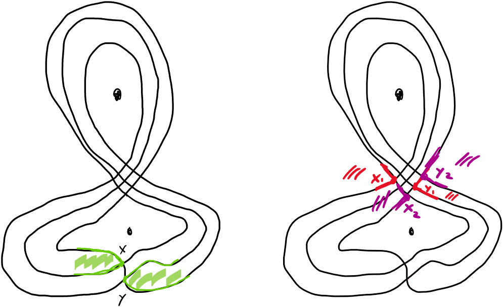
Figure 12: Left: The filled bigon with marked points $x$ and $y$ is not singular, and therefore not immersed in the sense of Definition 2.7. Right: The bigon with marked points $x_{1},y_{1}$ (resp. $x_{2},y_{2}$) is immersed (in fact, embedded) and the loop is not taut. Placing an additional puncture at infinity removes them and makes the loop taut.

Remark 2.9 (unicity of mobidiscs).

For a loop $\gamma\colon\mathbb{S}\looparrowright\mathbb{F}_{P}$ every immersed monorbigon $K$ of gives rise to at most two mobidiscs, and exactly one when $\mathbb{F}\neq\mathbb{S}^{2}$.

After choosing a base point $\infty$ in a region adjacent to a segment of $\gamma(K)$, either on the right ($s=+1$) or on the left ($s=-1$), the mobidiscs are among the two sets of regions $R(K,s)$ around which $\gamma(K)$ has a winding number of the same sign as $s$.

Remark 2.10 (non-unicity of extensions).

Note however that an immersed monorbigon $K$ of $\gamma$ can extend to several non-isotopic immersions $\iota\colon\mathbb{D}\looparrowright\mathbb{F}$ which define the same mobidisc. A famous example given by Milnor is depicted in Figure 13.

Given a loop in a surface, the description and computation of all its extensions to immersions of a disc had been raised by Hopf and Thom [Tho59]. It was first solved by Blank when $\mathbb{F}=\mathbb{R}^{2}$ [Bla67, Poé95], and generalised to other surfaces in [Fri10].

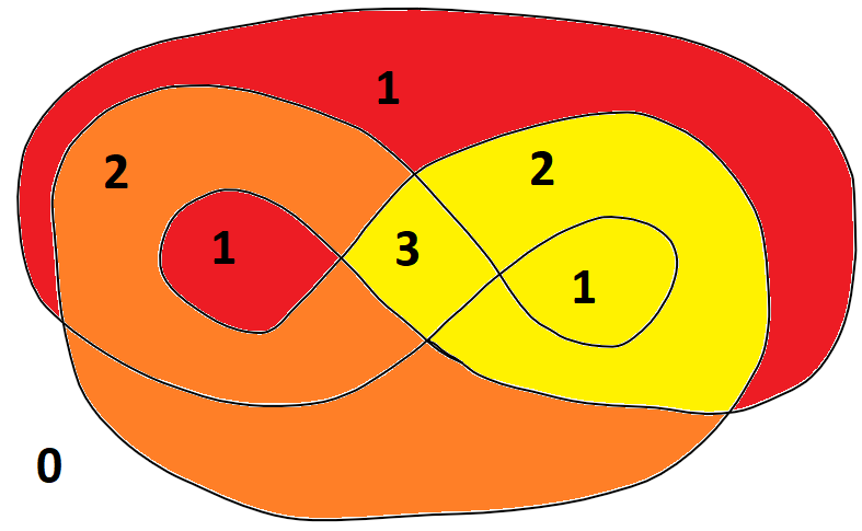
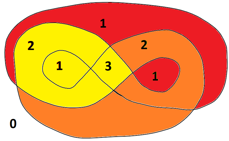
Figure 13: The “Milnor doodle” bounds an immersed disk in two different ways. When viewed from above, the yellow portions are the closest whereas the red portions are the farthest. The numbers in each region correspond to the local degree of the immersion - note that they agree in both cases.

The main result in this subsection is just improving on [HS85, Theorem 4.2].

Theorem 2.11 (taut loops have no immersed monorbigons).

Consider a closed oriented surface $\mathbb{F}$ together with a set of points $P\subset\mathbb{F}$, and a loop $\gamma\colon\mathbb{S}\looparrowright\mathbb{F}_{P}$.

The loop $\gamma\looparrowright\mathbb{F}_{P}$ is not taut if and only if it has an immersed monorbigon.

The proof will make use of another theorem by Hass–Scott [HS94].

Theorem 2.12 (curve shortening flow).

If two loops $\alpha,\beta\colon\mathbb{S}\looparrowright\mathbb{F}_{P}$ are homotopic, then there is a sequence of isotopies and Reidemeister moves $R1,R2,R3$ which never increase the number of double-points leading from one to the other.

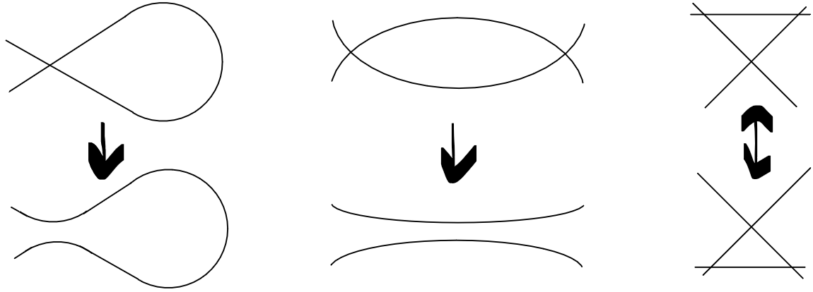
Figure 14: Reidemeister moves which do not increase the number of double-points. From left to right: $R1$, $R2$, $R3$.

Proof.

$\impliedby$ If $\gamma$ has an immersed monorbigon $K$, then $\gamma(K)$ is null-homotopic in a neighborhood of the union of regions of an associated mobidisc, implying that $\gamma$ is homotopic to a loop with strictly less double-points.

$\implies$ Let $\Xi$ be the set of loops $\gamma\colon\mathbb{S}\looparrowright\mathbb{F}$ in an oriented surface, with no immersed monorbigons, but which are still not taut. Suppose that $\Xi$ is non empty, and choose $\gamma$ in the subset $\Xi_{m}$ having the smallest number of double-points (irrespective of $\mathbb{F}$).

By [HS85, Theorem 4.2] the loop $\gamma$ has a singular monorbigon $K=I$ or $K=I\sqcup J$. Let $\alpha$ be the restriction of $\gamma$ to $K$, it has $1$ or $2$ marked points $\gamma(\partial K)$.

We claim that the only double-points of $\gamma$ are those of $\alpha$ and the marked points. This follows from the minimality assumption: if we consider the loop $\gamma_{0}$ in $\mathbb{F}_{0}$ obtained from $\alpha$ by adding monogons at the marked points and punctures in these monogons, then this $\gamma_{0}$ belongs to $\Xi_{m}$ (its number of double-points is no bigger than that of $\gamma$).

We know that $\alpha$ has double-points, because otherwise $\gamma$ would thus have an embedded monorbigon, which is in particular immersed.

Since $\alpha$ is null-homotopic, we know by [HS85, Theorem 2.7] that it must bound an embedded monorbigon. Since $\gamma$ does not contain immersed monorbigons, the embedded monogon or bigon for $\alpha$ must contain at least $2$ or $1$ of the marked points (in the sense that the marked points belong to the intervals at the source of $\alpha$).

By Theorem 2.12 there is a sequence of $R3$ moves from $\alpha$ to a loop $\alpha^{\prime}$ having a region $A$ of degree $1$ or $2$ which contains at least $2$ or $1$ marked points. These moves lift to $R3$ moves on $\gamma$, yielding a loop $\gamma^{\prime}$ with the same number of double-points.

The new loop $\gamma^{\prime}$ which is $R3$ equivalent to $\gamma$ must still belong to $\Xi_{m}$. Indeed, it is homotopic to $\gamma$ and has the same number of double-points, in particular it is not taut, yet it does not contain any immersed monorbigon since otherwize by inverting the sequence of $R3$ moves, we would have an immersed monorbigon for $\gamma$.

To summarise, we constructed a loop $\gamma^{\prime}\in\Xi_{m}$ with a singular bigon $\alpha^{\prime}$, which has a region $A$ of degree $1$ or $2$ whose edges contain at least $2$ or $1$ marked points of $\gamma^{\prime}$. Performing the $R1$ or $R2$ move on $\alpha^{\prime}$ associated to the region $A$ yields a new loop $\alpha^{\prime\prime}$, and this lifts to a sequence of $R3$ moves on $\gamma^{\prime}$ yielding a new loop $\gamma^{\prime\prime}$. But $\gamma^{\prime\prime}$ has less double-points than $\gamma^{\prime}$, so by minimality it must have an immersed monorbigon, and inverting the $R3$ move from $\gamma^{\prime\prime}$ to $\gamma^{\prime}$ reveals an immersed monorbigon in $\gamma^{\prime}$: that is a contradiction. ∎

2.3 Reducing pin the loop to a boolean formula

In this subsection we fix a filoop $\gamma\colon\mathbb{S}\to\mathbb{F}$ corresponding framed chord diagram $C$, as in subsection 2.1. We label the singular points at the source of $\gamma$ by the framed letters of $C$, and the double-points of $\gamma$ by the set $V$ of unframed letters of $C$.

Let us first reformulate Theorem 2.11 in terms of pinning sets.

Theorem 2.13 (pinning mobidiscs).

For a filoop $\gamma\colon\mathbb{S}\looparrowright\mathbb{F}$ with regions $R$, a subset of regions $P\in\operatorname{\mathcal{P}}(R)$ is pinning if and only if it intersects mobidisc $D\in\operatorname{MoB}(\gamma)$.

Algorithm 2.14 (computing mobidiscs).

For a filoop $\gamma\colon\mathbb{S}\looparrowright\mathbb{F}$, we can construct its collection of mobidiscs $\operatorname{MoB}(\gamma)\subset\operatorname{\mathcal{P}}(R)$ in time $O(\operatorname{Card}(V)^{2}\operatorname{Card}(R)^{2})$.

Proof.

We first apply algorithm 2.5 to find all singular monorbigons. (Recall for later purposes that a singular monorbigon $K$ satisfies $\gamma(K)\equiv 0\in H_{1}(\mathbb{F};\mathbb{Z})$.) For each singular monorbigon $K$, we check in time $O(\operatorname{Card}(R))$ if $\gamma(K)$ bounds an immersed disc using [Fri10, Theorem 3.1.5 and Theorem 3.2.4 and Theorem 5.2.7]. We have thus computed $O(\operatorname{Card}(V)^{2})$ immersed monorbigons in time $O(\operatorname{Card}(V)^{2}\operatorname{Card}(R)^{2})$.

Then, for every immersed monorbigon $K$ and every $s\in\{-1,+1\}$, we compute the subset of regions $R(K,s)\subset R$ defined in Remark 2.9 using winding numbers. We have thus $O(\operatorname{Card}(V)^{2})$ sets of regions, each one computed in time $O(\operatorname{Card}(R)^{2})$. (Alternatively, the regions $R(K,s)$ can be defined and constructed inductively by adding layers of regions as follows. The regions in the first layer are incident to the subloop $\gamma(K)$ on the side $-s$. The regions in the layer $l+1$ are adjacent to those in the layer $l$ on the side $-s$. We add layers inductively until reaching an empty layer.)

Finally the set $R(K,s)\subset\operatorname{\mathcal{P}}(R)$ is a mobidisc when the union of its closed regions has an interior that is connected and simply connected. This condition can be verified in $\operatorname{Card}(R)$ steps (see Remark 1.2). We thus computed the collection $\operatorname{MoB}(\gamma)\subset\operatorname{\mathcal{P}}(R)$ of all mobidiscs in time $O(\operatorname{Card}(V)^{2}\operatorname{Card}(R)^{2})$. ∎

Let us now reformulate the LooPin problem as a satisfyability problem.

Definition 2.15 (formulae and satisfying assignments).

Consider a set of variables $x_{1},\dots,x_{r}$ which may take boolean values $\{\operatorname{1},\operatorname{0}\}$. A formula $\phi$ is an expression in the variables $x$ involving negations $\neg$, disjunctions $\wedge$, conjunctions $\vee$ (and parentheses).

Evaluating the variables $x$ at $\xi\in\{\operatorname{1},\operatorname{0}\}^{r}$ yields a value $\phi(\xi)\in\{\operatorname{1},\operatorname{0}\}$ for the formula $\phi$. Such an assignment $\xi$ of the variables $x$ is said to satisfy $\phi$ when $\phi(\xi)=\operatorname{1}$.

Two formulae $\phi,\phi^{\prime}$ on the set of variables $x$ are called logically equivalent when their evaluations on every assignment $\xi$ of the variables $x$ are equal $\phi(\xi)=\phi^{\prime}(\xi)$.

Every formula is equivalent to a conjunctive normal form. (One can also show that there is an essentially unique “minimal” conjunctive normal form.)

Definition 2.16 (conjunctive normal form).

Consider boolean variables $x_{1},\dots,x_{r}$.

A clause is a formula of the form $l_{1}\vee\dots\vee l_{k}$ where each $l_{j}$ is a literal, namely a variable $x_{t}$ or its negation $\neg x_{i}$. A conjunctive normal form (abbreviated CNF) is a formula which is conjunction $c_{1}\wedge\dots\wedge c_{m}$ of clauses $c_{j}$. A conjunctive normal form is called positive when none of the clauses feature negated variables.

Definition 2.17 (solution semi-lattice).

Consider a positive conjunctive normal form $\phi$ over a set of boolean variables $x_{1},\dots,x_{r}$. For an assignment $\xi$ of $x$ satisfying $\phi$, we call $\{x_{i}\mid\xi_{i}=\operatorname{1}\}\in\operatorname{\mathcal{P}}(x)$ a solution of $\phi$.

The solutions of $\phi$ form a sub-poset $\mathcal{S}(\phi)\subset\operatorname{\mathcal{P}}(x)$ which is closed by union (that is a join-semi-lattice) and contains the set of all elements $\{x_{1},\dots,x_{r}\}$.

Remark 2.18 (hyper-graph vertex-cover).

The solutions of a positive conjunctive normal form correspond to the vertex-covers of the hyper-graph whose vertices are indexed by the variables and hyper-edges correspond to the clauses.

We will only need to consider conjunctive normal forms which are positive.

Definition 2.19 (mobidisc formula).

To a loop $\gamma\colon\mathbb{S}\to\mathbb{F}$ we associate its mobidisc formula: it is the positive conjunctive normal form on the set of boolean variables indexed by its set of regions whose clauses correspond to $\operatorname{MoB}(\gamma)\subset\operatorname{\mathcal{P}}(R)$.

Question 2.20.

Can we describe, among all positive conjunctive normal forms, the mobidisc formulae arising from filoops, and from those in genus $g$?

The next subsection will show that this class is complex even when $g=0$: the task of finding (the cardinal of) an optimal solutions is strongly NP-complete.

We may now reformulate Theorem 2.13 as follows.

Theorem 2.21 (pinning sets of a filoop = solutions of its mobidisc formula).

The pinning sets of a loop correspond to the solutions of its mobidisc formula.

In particular, the pinning semi-lattice of a loop is isomorphic to the solution semi-lattice of its mobidisc formula.

Hence the Algorithm 2.14 recovers the following corollary (which we already knew as a consequence of Corollary 1.10).

Corollary 2.22 (LooPiNum is NP).

The LooPiNum problem, defined by

• A filling loop $\gamma\colon\mathbb{S}\looparrowright\mathbb{F}$, and an integer $p\in\mathbb{N}$.

• Does $\gamma$ have pinning number $\varpi(\gamma)\leq p$?

belongs to the class NP.

Remark 2.23 (SAT-solver).

Once the subset $\operatorname{MoB}(\Gamma)\subset\operatorname{\mathcal{P}}(R)$ has been computed in time $\operatorname{Card}(V)^{2}\operatorname{Card}(R)$ as in the algorithm 2.14, one may send it to a SAT-solver designed to compute optimal solutions to positive conjuctive normal forms.

In practise, the current SAT-solvers for these problems are surprisingly fast.

Remark 2.24 (just for loops).

The Algorithm 2.14 relies on Theorems 2.11 and 2.13 which only hold for loops, and do not have obvious generalisations to multiloops.

Indeed, [HS85, figure 0.1] exhibits a multiloop with $2$ strands inside an annulus which is not taut, but that does not bound any singular bigon involving both strands.

After adding a puncture as in Figure 15, we obtain a multiloop in a thrice-punctured sphere which is not taut, but now has no singular monorbigons at all.

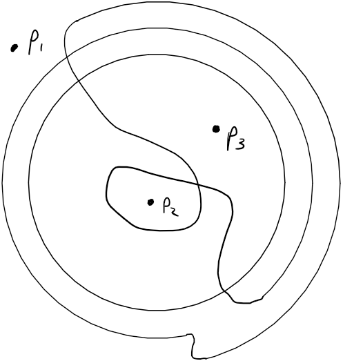
Figure 15: A multiloop $\mathbb{S}\sqcup\mathbb{S}\looparrowright\mathbb{S}^{2}\setminus\{p_{1},p_{2},p_{3}\}$ which is not taut, but having no singular monorbigons.

This is why this subsection restricts to loops, and we wonder if the MultiLooPiNum problem belongs to a stricter larger sub-complexity class than LooPiNum.

2.4 Reducing planar vertex-cover to pin-the-loop

We now show that the PinNum problem for loops is NP-hard by reduction from the following decision problem which is known to be NP-hard by [GJS76][Theorem 2.7].

Definition 2.25 (Planar vertex cover).

The planar vertex cover problem has:

• A planar graph $G=(V,E)$ and a positive integer $k\leq\operatorname{Card}(V)$.

• Is there $U\subset V$ with $\operatorname{Card}(U)\leq k$ such that for all $\{v_{1},v_{2}\}\in E$, at least one of $v_{1}$ and $v_{2}$ belongs to $U$?

Remark 2.26 (Plane connected).

For our purposes, the planar vertex cover problem has the same complexity as its restriction to connected plane graphs.

On the one hand, the vertex covers of a graphs correspond to the disjoint union of the vertex covers of each connected components.

On the other hand, there are linear time algorithms [HT74] which given a graph, decide if it is planar and when so compute a plane embedding (encoded as a cyclic order of the edges around each vertex).

Algorithm 2.27 (planar vertex cover reduces to LooPinNum).

The planar vertex cover problem admits a polynomial reduction to the LooPinNum problem.

More precisely, there exists a polynomial time algorithm which to a planar graph $G=(V,E)$ associates a plane loop $\gamma\colon\mathbb{S}\to\mathbb{D}$ with $O(\operatorname{Card}(E)^{2})$ double-points, such that the $k$-vertex-covers of $G$ are in one to one correspondence with the $(2\operatorname{Card}(E)+k)$-pinning-sets of $\gamma$.

Proof outline.

Given an instance $(G=(V,E),k\in\mathbb{N})$ of planar vertex cover, we will construct an instance $(\gamma,2\operatorname{Card}(E)+k)$ of LooPinNim, and show that they yield equivalent problems. As mentioned in Remark 2.26 we may assume that $G$ is connected and endowed with a plane embedding in $\mathbb{B}(0,1)$.

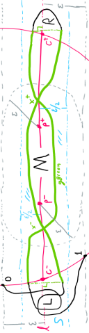
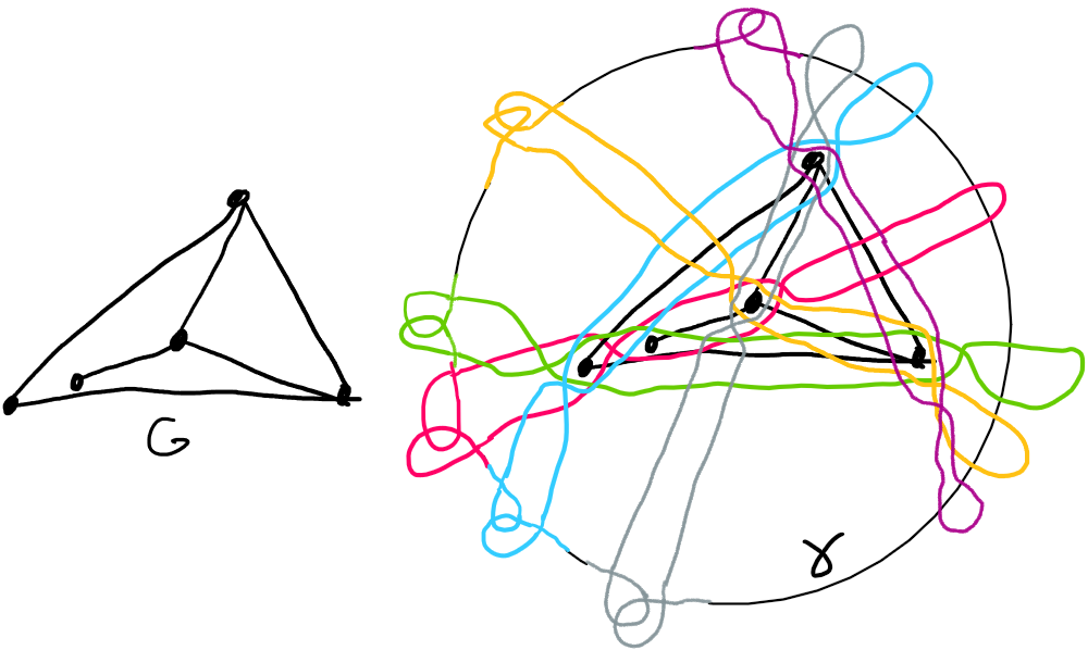
Figure 16: Assembling edge gadgets around a graph.

Following the example in Figure 16, we will associate to every edge $e\in E$ an edge-gadget $g_{e}$, and connect them all to together through the boundary circle $\partial\mathbb{B}(0,1)$ to form a loop $\gamma$. The technical part of the construction is to separate the gadgets adequately so as to ensure to ensure the genericity of $\gamma$ and the equivalence of the two problems. In particular, we will have a correspondence (1) between the vertices of $G$ and the maximal nonempty intersections of certain edge-bigons of $\gamma$. ∎

Construction of the loop.

Let us now perform the construction in detail.

We work in the euclidean plane $\mathbb{R}^{2}$ with distance function $d$. For a subset $X\subset\mathbb{R}^{2}$ and $\epsilon\in\mathbb{R}_{+}$ we denote by $\operatorname{\mathbb{B}}(X,\epsilon)$ the $\epsilon$-neighbourhood of $X$.

We first define the edge-gadget precisely.

Definition 2.28 (Edge gadget).

The edge gadget is specified by $\epsilon\in(0,1)$ and a chord $c=(c^{-},c^{+})\subset\mathbb{B}(0,1)$ containing a segment $[p^{-},p^{+}]$ such that $\operatorname{\mathbb{B}}([p^{-},p^{+}],\epsilon)\subset\operatorname{\mathbb{B}}(0,1)$.

The edge gadget with this data is a smooth immersion $g:[-1,+1]\looparrowright\operatorname{\mathbb{B}}(c,\epsilon)$ in the isotopy class of that shown in Figure 17 which satisfies the following constraints:

• Its image $\operatorname{im}(g)$ intersects both components of $\operatorname{\mathbb{B}}(c,\epsilon)\setminus\operatorname{\mathbb{B}}(0,1)$, and its endpoints are $\{g(-1),g(+1)\}=\partial\operatorname{\mathbb{B}}(0,1)\cap\partial\operatorname{\mathbb{B}}(c^{-},\epsilon)$.

• Let $T$ be the smallest rectangle containing $\overline{\operatorname{\mathbb{B}}(0,1)}\cap\overline{\operatorname{\mathbb{B}}(c,\epsilon/2)}$, and define the between-portion of $g$ by $\operatorname{\between}=\operatorname{im}(g)\cap T$. We insist that $g^{-1}(T)$ has exactly two connected components and that no tangent lines to $\operatorname{\between}$ are normal to $c$.

• The self-intersections $x^{\pm}$ of $\operatorname{\between}$ satisfy $x^{-}\in\operatorname{\mathbb{B}}(p^{-},\epsilon)$ and $x^{+}\in\operatorname{\mathbb{B}}(p^{+},\epsilon)$.

To such a gadget are associated the bigons $L$ and $M$, and region $R$ as in Figure 17.

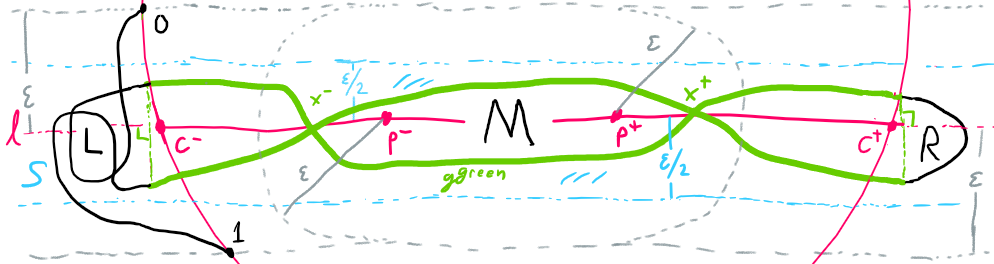
Figure 17: The edge gadget in metric details.

Now to a connected plane graph $G\hookrightarrow\mathbb{B}(0,1)$ we associate a loop $\gamma\colon\mathbb{S}\looparrowright\mathbb{R}^{2}$, by positioning edge-gadgets meticulously and assembling them. One may check that every step of the construction can be performed in polynomial time.

1. According to [Wag36, F4́8, Ste51], we may construct in polynomial time a plane embedding of $G\hookrightarrow\operatorname{\mathbb{B}}(0,1)$ with straight edges. We may also assume (after a generic perturbation of the vertices) that no edges of $G$ are parallel. Each edge of $G$ spans a line in $\mathbb{R}^{2}$, and we rescale the embedding so that all intersection points between such lines lie inside $\operatorname{\mathbb{B}}(0,1)$.

2. Fix a total order on the vertices $V$ and orient each edge $e\in E$ from its smallest vertex $e^{-}\in V$ to its largest vertex $e^{+}\in V$. Each oriented edge $e\in E$ generates an oriented affine line intersecting $\operatorname{\mathbb{B}}(0,1)$ along an oriented chord $c_{e}=(c_{e}^{-},c_{e}^{+})$. By 1, we have $2\operatorname{Card}(E)$ distinct points $c_{e}^{\pm}\in\partial\operatorname{\mathbb{B}}(0,1)$ on the unit circle.

3. Choose $\epsilon>0$ such that $\operatorname{\mathbb{B}}(G,\epsilon)\subset\operatorname{\mathbb{B}}(0,1)$, and $\forall e_{1},e_{2}\in E$ with $e_{1}\neq e_{2}$ we have $\operatorname{\mathbb{B}}(c_{e_{1}},\epsilon)\cap\operatorname{\mathbb{B}}(c_{e_{2}},\epsilon)\subset\operatorname{\mathbb{B}}(0,1)$ (possible by 1), and for all $\{e_{i}\}_{i=1}^{k}\subset E$:

   $$\bigcap_{i=1}^{k}\mathbb{B}(e_{i},\epsilon)\quad\text{retracts by deformation onto}\quad\bigcap_{i=1}^{k}e_{i}.$$

4. For each $e\in E$ we embed an edge gadget $g_{e}$ with data $\epsilon$ and $(c_{e}^{-},e^{-},e^{+},c_{e}^{+})$. Step 3 implies that the input conditions are satisfied and the only intersection points between different gadgets lie inside $\cup_{e\in E}\operatorname{\between}_{e}$.

5. For each $g_{e}$, perform a surgery on $\partial\mathbb{B}(0,1)$ replacing the arc $\partial\mathbb{B}(0,1)\cap\mathbb{B}(c_{e}^{-},\epsilon)$ between its end-points $g_{e}(\pm 1)$, with $g_{e}$. Fix an orientation of the resulting closed loop and call it $\gamma$.

6. We now perturb $\gamma$ into a generic position.

   • We remove tangency points associated to distinct gadgets by compressing gadgets as follows.

     Let $\theta(\ell_{1},\ell_{2})\in[0,\pi/2]$ be the smallest angle between two unoriented lines $\ell_{1}$ and $\ell_{2}$, and let $\ell_{p}$ be the tangent line to a gadget at a point $p$.

     For each gadget $g_{e}$, let $\phi_{e}=\max\{\theta(\ell_{p},\ell_{e})\mid p\in\operatorname{\between}_{e}\}$ which exists in $(0,\pi/2)$ by compactness, and let $\phi_{e}=\max\{\phi_{e}\mid e\in E\}$.

     The minimal angle $\rho=\min\{\theta(c_{e_{1}},c_{e_{2}})\mid e_{1},e_{2}\in E,e_{1}\neq e_{2}\}$ between two distinct chords is positive by 1.

     For an abstract gadget $g$ there is a diffeomorphism of $\mathbb{R}^{2}$ with support in $\operatorname{\mathbb{B}}(c,\epsilon/2)$ which acts by contraction towards $c$ along lines normal to $c$ (preserving each normal line to $c$, and the foliation of lines parallel to $c$). For each gadget $g_{e}$ we apply a suitably high power of this contraction prior to embedding $g_{e}$ so that $\phi_{e}<\rho/2$ after embedding, thus $\phi<\rho/2$.

     This ensures that $\gamma$ has no tangency points while preserving all other properties of the construction.

   • What remains are possible isolated multiple points. We resolve them locally into transverse double-points so as to preserve the key intersection property below.

The polynomial construction of $\gamma$ is finished. Note that for all $e\in E$ we have a bigon $M_{e}$ satisfying $e\subset M_{e}\subset\operatorname{\mathbb{B}}(e,\epsilon)$ whence by 3, for all $\{e_{i}\}_{i=1}^{k}\subset E$:

$$\bigcap_{i=1}^{k}M_{e_{i}}\quad\text{retracts by deformation onto}\quad\bigcap_{i=1}^{k}e_{i}.$$ (1)

The latter intersection is empty, unless all the $e_{i}$ share a common vertex $v$. ∎

Proof of the equivalence.

We now show that the instances $(G=(V,E),k)$ of planar vertex cover and $(\gamma,2\operatorname{Card}(E)+k)$ of LooPinNim yield equivalent problems.

By construction, every mobidisc of $\gamma$ contains at least one of the $3\operatorname{Card}(E)$ bigons $L_{e}$, $M_{e}$ or $R_{e}$ for $e\in E$. It follows from Theorem 2.13 and equation (1) that $\gamma$ is pinned if and only if both of the following hold:

1. for every $e\in E$ there is a pin in $L_{e}$ and a pin in $R_{e}$

2. for every $v\in V$ there is a pin in at least one of the $M_{e}$ for edges $e\supset v$

It follows that there is a bijective correspondence between the optimal vertex covers of $G$ and the optimal pinning sets of $\gamma$, which proves the desired equivalence.

This completes the proof of the reduction 2.27. ∎

Corollary 2.29.

The problem LooPinNim is strongly NP-hard.

Proof.

The planar vertex cover problem is strongly NP-complete [GJ78][§3.7]. The Algorithm 2.27 returns a loop whose size is proportional to the size of its input planar graph. Hence the LooPinNum problem is strongly NP-hard. ∎

Remark 2.30.

The planar vertex cover problem remains NP-complete even for graphs with $\max$-degree $3$ by [GJ77][Lemma 1], but such an assumption would not simplify our construction.

In fact, our construction could be adapted without significant modification to work for any graph (planar or not), but the proof would be more involved.

3 The pinning semi-lattice of a multiloop

3.1 The structure of the pinning semi-lattice

Definition 3.1 (pinning semi-lattice).

Consider a multifiloop $\gamma\colon\sqcup_{1}^{s}\mathbb{S}\looparrowright\mathbb{F}$.

Its collection of pinning sets is closed under taking unions and supersets: it forms a join semi-lattice. We call it the pinning semi-lattice of $\gamma$.

Remark 3.2.

The pinning semi-lattice is determined by its set of minimal elements (which form a maximal anti-chain).

Every pinning semi-lattice has a unique upper bound (the set of all regions).

By Theorem 2.29, pinning semi-lattices are hard to compute in general.

Question 3.3 (number of strands).

By Theorem 2.21, the pinning semi-lattice of a loop $\gamma$ with regions $R$ is isomorphic to the solution semi-lattice of its mobidisc formula $\operatorname{MoB}(\gamma)\subset\operatorname{\mathcal{P}}(R)$. The pinning semi-lattice of multiloops is more mysterious.

Is there a topological notion generalising mobidiscs to multiloops, which would yield a basis for the pinning semi-lattice?

Can we compute or estimate lower bounds for the number of strands of a multiloop from its pinning semi-lattice?

Question 3.4 (structure of pinning semi-lattices).

Which join semi-lattices arise as pinning semi-lattices of filling loops or multiloops?

How do pinning semi-lattices of multifiloops behave under Reidemeister moves, flypes, and crossing resolutions? We will see in Figures 18 and 19 that the pinning number can change under $R3$-moves and flypes on indecomposible loops in the sphere.

How do pinning semi-lattices of loops behave under the operations of spheric-sums and toric-sums introduced in [Sim23]?

3.2 Variance under Reidemeister triangle moves and flypes

As mentioned in [dMRST21], upper bounds on the complexity of deciding numerical invariants of knots and links are often elusive. In contrast, the present work shows that certain subtle measures of the complexity of multiloops are more tractable.

One may thus hope to interpret certain link invariants in terms of certain numerical invariants of multiloops related to the pinning problem (such as the pinning number, the number of optimal or minimal pinning sets, etc.).

For this one must first find a way to represent links by decorated multiloops and show that the pinning quantities only depend on the link. The next paragraphs records the failure of two such approaches.

Lifting multiloops to legendrian links: pinning varies under $R3$-moves

A multiloop $\gamma\colon\sqcup_{1}^{s}\mathbb{S}^{1}\looparrowright\mathbb{F}$ lifts to a unoriented Legendrian link in the projective tangent bundle $\overline{\gamma}\colon\sqcup_{1}^{s}\mathbb{S}\looparrowright\overline{\mathbb{F}}$.

Two such links are isotopic if and only if their projections differ by sequences of certain combinatorial moves, including Reidemeister moves $R3$.

If a quantity related to the pinning problem for multiloops were invariant under the Reidemeister move $R3$, then one may hope to relate it to an isotopy invariant of that Legendrian link. Alas, the pinning number is not, as one can see in Figure 18.

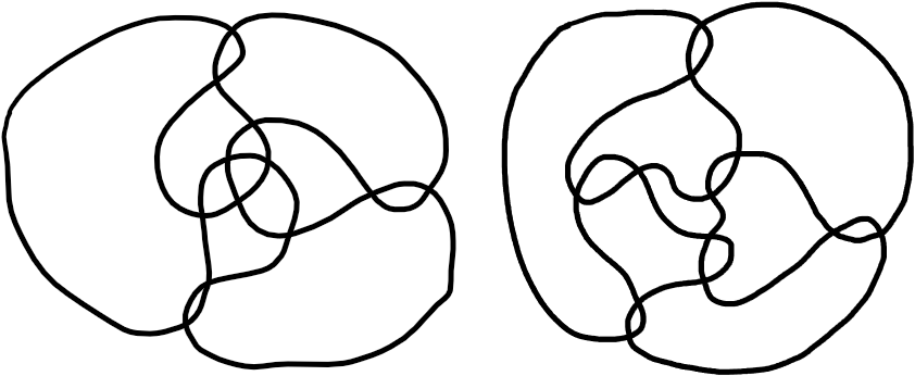
Figure 18: The pinning number is not invariant under $R3$ moves: [SS24, link].

Lifting multiloops to alternating links: pinning varies under flypes

A multiloop $\gamma\colon\sqcup_{1}^{s}\mathbb{S}^{1}\looparrowright\mathbb{R}^{2}$ yields two alternating diagrams for a link $\hat{\gamma}\colon\sqcup_{1}^{s}\looparrowright\mathbb{R}^{2}\times\mathbb{R}$ which are related by a mirror image reflection.

An oriented link may have several alternating diagrams, by the Tait flyping conjecture proved by Thistlethwaite–Menasco [MT91, MT93], the indecomposible alternating diagrams of a prime link are related by sequences of flypes.

Hence if a pinning-quantity of indecomposible multiloops in the sphere is invariant under flypes moves, then one may hope to relate it to an isotopy invariant of prime alternating links. Alas, the pinning number is not, as one can see in Figure 19.

Figure 19: The pinning number may change under flypes & mutations: [SS24, link].

3.3 Databases of pinning semi-lattices and related quantities

Using plantri [BM] and the Algorithm 0.5, we computed the pinning semi-lattices of all irreducible indecomposible spherical multiloops with at most $14$ regions (unoriented and up to reflection), and the statistics of certain numerical parameters. The number of such loops follows [OEI24, A264759] and the number of multiloops follows [OEI24, A113201]. The results are available in a catalog at this link. Let us mention a few observations.

Remark 3.5 (region degrees).

On average, there is a strong correlation between the region’s degrees and probability of being pinned. It is false however that the average degree increases from optimal pinning sets to minimal pinning sets. See Figure 20.

Figure 20: Left and center: Loops with the the property that the average degree of every optimal pinning set is larger than the average degree of every minimal, suboptimal pinning set. Right: A loop with the property that the sum of degrees of some optimal pinning set is greater than the sum of degrees of some minimal, suboptimal pinning set. See [SS24, this link] (created with SnapPy [CDGW]).

One may turn the previous remark into a heuristic leading to efficient algorithms computing almost optimal pinning sets of most multiloops.

Remark 3.6 (heuristics).

The strategy consisting in solving the boolean formula whose clauses correspond to the regions bounded by embedded monorbigons often yields an almost pinning set.

One may construct arbitrarily complicated loops with fixed pinning number $\varpi\geq 3$ by taking long words in $\mathcal{F}_{\varpi-1}$ and corresponding geodesics in a surface of genus $0$ and $\varpi$ punctures. However for long geodesics, the regions to be pinned become obvious.

Example 3.7 (smallest multiloops with $\deg\geq 3$).

Using lemma 1.4 and an exhaustive computation we found all multiloops in the sphere with at most $16$ regions, all of which have degree $\geq 3$. The number of such multiloops follows [OEI24, A078666]. See the catalog.

The pinning semi-lattices of those with at most $12$ regions are represented in Figure 4. In the figures that follow, optimal pinning sets are labelled with capital letters and shades of red, and the other minimal pinning sets are labelled with lowercase letters and shades of green. For better visibility, we do not plot the entire pinning semi-lattice; rather, the sub-semi-lattice generated by (taking unions of) minimal pinning sets, together with the set of all regions. The heights of vertices in the semi-lattice (and the labels therein) correspond to their cardinals. A lighter edge emphasises a greater difference between its endpoint’s cardinals.

References

- [AHT02] Ian Agol, Joel Hass, and William Thurston. 3-manifold knot genus is NP-complete. In Proceedings of the Thirty-Fourth Annual ACM Symposium on Theory of Computing, pages 761–766. ACM, New York, 2002.
- [BHW22] Jonathan Bowden, Sebastian Wolfgang Hensel, and Richard Webb. Quasi-morphisms on surface diffeomorphism groups. J. Amer. Math. Soc., 35(1):211–231, 2022.
- [Bla67] S. J. Blank. Extending immersions of the circle. Ph.D. dissertation, 1967. Brandeis University, Waltham, MA.
- [BM] Gunnar Brinkmann and Brendan McKay. Plantri and fullgen, programs for generating planar graphs of specified types. Available at https://users.cecs.anu.edu.au/~bdm/plantri/(08/04/2024).
- [BS84] Joan S. Birman and Caroline Series. An algorithm for simple curves on surfaces. J. London Math. Soc. (2), 29(2):331–342, 1984.
- [BS87] Joan S. Birman and Caroline Series. Dehn’s algorithm revisited, with applications to simple curves on surfaces. In Combinatorial group theory and topology (Alta, Utah, 1984), volume 111 of Ann. of Math. Stud., pages 451–478. Princeton Univ. Press, Princeton, NJ, 1987.
- [Car91] J. Scott Carter. Classifying immersed curves. Proc. Amer. Math. Soc., 111(1):281–287, 1991.
- [CDGW] Marc Culler, Nathan M. Dunfield, Matthias Goerner, and Jeffrey R. Weeks. SnapPy, a computer program for studying the geometry and topology of -manifolds. Available at http://snappy.computop.org (08/04/2024).
- [CL87] Marshall Cohen and Martin Lustig. Paths of geodesics and geometric intersection numbers. I. In Combinatorial group theory and topology (Alta, Utah, 1984), volume 111 of Ann. of Math. Stud., pages 479–500. Princeton Univ. Press, Princeton, NJ, 1987.
- [DL19] Vincent Despré and Francis Lazarus. Computing the geometric intersection number of curves. J. ACM, 66(6):Art. 45, 49, 2019.
- [dMRST21] Arnaud de Mesmay, Yo’av Rieck, Eric Sedgwick, and Martin Tancer. The unbearable hardness of unknotting. Adv. Math., 381:Paper No. 107648, 36, 2021.
- [dMSS20] Arnaud de Mesmay, Marcus Schaefer, and Eric Sedgwick. Link crossing number is NP-hard. J. Knot Theory Ramifications, 29(6):2050043, 15, 2020.
- [F4́8] István Fáry. On straight line representation of planar graphs. Acta Univ. Szeged. Sect. Sci. Math., 11:229–233, 1948.
- [FM12] Benson Farb and Dan Margalit. A primer on mapping class groups, volume 49 of Princeton Mathematical Series. Princeton University Press, Princeton, NJ, 2012.
- [Fri10] Dennis Frisch. Classification of immersions which are bounded by curves in surfaces. Ph.D. dissertation, 2010.
- [GJ77] M. R. Garey and D. S. Johnson. The rectilinear Steiner tree problem is NP-complete. SIAM J. Appl. Math., 32(4):826–834, 1977.
- [GJ78] M. R. Garey and D. S. Johnson. “Strong” NP-completeness results: motivation, examples, and implications. J. Assoc. Comput. Mach., 25(3):499–508, 1978.
- [GJS76] M. R. Garey, D. S. Johnson, and L. Stockmeyer. Some simplified NP-complete graph problems. Theoret. Comput. Sci., 1(3):237–267, 1976.
- [HLP99] Joel Hass, Jeffrey C. Lagarias, and Nicholas Pippenger. The computational complexity of knot and link problems. J. ACM, 46(2):185–211, 1999.
- [HS85] Joel Hass and Peter Scott. Intersections of curves on surfaces. Israel J. Math., 51(1-2):90–120, 1985.
- [HS94] Joel Hass and Peter Scott. Shortening curves on surfaces. Topology, 33(1):25–43, 1994.
- [HT74] John Hopcroft and Robert Tarjan. Efficient planarity testing. J. Assoc. Comput. Mach., 21:549–568, 1974.
- [KT21] Dale Koenig and Anastasiia Tsvietkova. NP-hard problems naturally arising in knot theory. Trans. Amer. Math. Soc. Ser. B, 8:420–441, 2021.
- [Lac21] Marc Lackenby. The efficient certification of knottedness and Thurston norm. Adv. Math., 387:Paper No. 107796, 142, 2021.
- [LZ04] Sergei K. Lando and Alexander K. Zvonkin. Graphs on surfaces and their applications, volume 141 of Encyclopaedia of Mathematical Sciences. Springer-Verlag, Berlin, 2004. With an appendix by Don B. Zagier, Low-Dimensional Topology, II.
- [MT91] William W. Menasco and Morwen B. Thistlethwaite. The Tait flyping conjecture. Bull. Amer. Math. Soc. (N.S.), 25(2):403–412, 1991.
- [MT93] William Menasco and Morwen Thistlethwaite. The classification of alternating links. Ann. of Math. (2), 138(1):113–171, 1993.
- [NC01] Max Neumann-Coto. A characterization of shortest geodesics on surfaces. Algebr. Geom. Topol., 1:349–368, 2001.
- [OEI24] OEIS Foundation Inc. The On-Line Encyclopedia of Integer Sequences, 2024. Published electronically at http://oeis.org.
- [Poé95] Valentin Poénaru. Extension des immersions en codimension (d’après Samuel Blank). In Séminaire Bourbaki, Vol. 10, pages Exp. No. 342, 473–505. Soc. Math. France, Paris, 1995.
- [Rei62] Bruce L. Reinhart. Algorithms for Jordan curves on compact surfaces. Ann. of Math. (2), 75:209–222, 1962.
- [Sim23] Christopher-Lloyd Simon. Loops in surfaces, chord diagrams, interlace graphs: operad factorisations and generating grammars, 2023. Submitted for publication, arxiv version.
- [SL23] Alexander Schmidhuber and Seth Lloyd. Complexity-theoretic limitations on quantum algorithms for topological data analysis. PRX Quantum, 4:040349, Dec 2023.
- [SS24] Christopher-Lloyd Simon and Ben Stucky. LooPin - Code to accompany ’Pin the loop taut : a one-player topologame’, May 2024.
- [Ste51] S. K. Stein. Convex maps. Proc. Amer. Math. Soc., 2:464–466, 1951.
- [Tho59] R. Thom. Remarques sur les problèmes comportant des inéquations différentielles globales. Bulletin de la Société Mathématique de France, 87:455–461, 1959.
- [Wag36] K. Wagner. Bemerkungen zum vierfarbenproblem. Jahresbericht der Deutschen Mathematiker-Vereinigung, 46:26–32, 1936.