Dynamic Scattering Arrays for Simultaneous Electromagnetic Processing and Radiation in Holographic MIMO Systems
Abstract
To meet the stringent requirements of next-generation wireless networks, multiple-input multiple-output (MIMO) technology is expected to become massive and pervasive. Unfortunately, this could pose scalability issues in terms of complexity, power consumption, cost, and processing latency. Therefore, novel technologies and design approaches, such as the recently introduced holographic MIMO paradigm, must be investigated to make future networks sustainable.
In this context, we propose the concept of a dynamic scattering array (DSA) as a versatile 3D structure capable of performing joint wave-based computing and radiation by moving the processing from the digital domain to the electromagnetic (EM) domain. We provide a general analytical framework for modeling DSAs, introduce specific design algorithms, and apply them to various use cases. The examples presented in the numerical results demonstrate the potential of DSAs to further reduce complexity and the number of radiofrequency (RF) chains in holographic MIMO systems while achieving enhanced EM wave processing and radiation flexibility for tasks such as beamforming and single- and multi-user MIMO.
Index Terms:
Dynamic Scattering Arrays, Holographic MIMO; EM signal processing; superdirectivity.I Introduction
Next-generation wireless systems are expected to provide enhanced performance in terms of capacity, reduced latency, and new functionalities such as integrated sensing and communication [1, 2]. This trend is driving the investigation of fundamental limits using physically consistent models, new technologies, and novel design paradigms to approach them [3, 4, 5].
In this context, the recently introduced holographic communications paradigm is envisioned as a holistic way to manipulate, with unprecedented flexibility, the electromagnetic (EM) field generated or sensed by an antenna [6]. It involves designing innovative solutions capable of approaching the fundamental limits imposed by the wireless channel through the massive deployment of reconfigurable intelligent surfaces [7], extremely large antenna arrays (ELAA) [8], and large intelligent surfaces, also known as holographic MIMO [9, 10, 11].
In particular, holographic MIMO surfaces are envisioned as an efficient implementation of large antenna systems, advancing beyond massive MIMO and ELAAs using simplified and reconfigurable hardware that is reduced in size, cost and power consumption, and facilitate signal processing in the analog domain [11]. In holographic MIMO, the density of the antenna elements is increased, ideally approaching a continuous distribution, which allows for highly flexible manipulation of EM waves. Additionally, exploiting higher frequency bands, such as millimeter wave and THz, opens up the potential to utilize the extra degrees-of-freedom (DoF) provided by the channel in the radiating near-field propagation region, even under line-of-sight (LOS) conditions [12, 13, 14, 15, 16, 17]. Closely spaced antenna elements (below , with being the wavelength) do not significantly increase the exploitable DoF of the channel [18, 10]. Nevertheless, when the elements spacing is made very small, strong coupling occurs, and the gain of a linear array shifts from , as in conventional arrays, to , being the number of antenna elements, resulting in the so-called “superdirectivity” [19]. While achieving very narrow beams using size-limited antennas is highly desirable in many contexts, the superdirectivity effect is only obtained in the end-fire direction of the array and can lead to extremely high driving currents corresponding to high -factor values (and hence a lower bandwidth) [20].
The utilization of high-frequency bands in the millimeter wave and THz ranges, coupled with the integration of antennas with a very large number of elements, is pushing current technology towards insurmountable barriers in hardware complexity and power consumption. This issue, also known as digital bottleneck, poses serious challenges for the sustainability of future wireless networks. In MIMO-based systems, hybrid digital-analog solutions have been extensively explored to partially alleviate these issues by reducing the number of radiofrequency (RF) chains and the digital processing burden, albeit at the expense of flexibility [21].
A promising approach toward sustainability is to delegate part of the signal processing directly to the EM level, known as electromagnetic signal and information theory (ESIT) [22, 23, 24]. This can be achieved by designing reconfigurable EM environments [25] using novel EM metamaterials devices to perform basic processing functions (e.g., spatial first derivative) [26], RISs, or the recently introduced stacked intelligent metasurfaces [27]. However, SIMs do not fully exploit the possibilities offered by EM phenomena in antenna structures for processing and radiation, thereby inheriting some limitations of standard antenna arrays as will be detailed later.
To overcome the aforementioned issues, we put forth the idea of a dynamic scattering array (DSA) where EM processing and radiation are performed jointly “over the air” by using a few active antenna elements surrounded by a cloud of interacting programmable scatterers. As will be demonstrated, DSAs offer several advantages in terms of flexibility and size reduction while minimizing the number of RF chains required.
I-A Related State of the Art
The idea of introducing passive scattering elements close to an antenna to exploit mutual coupling in the reactive near-field region and shape its radiation properties dates back to the early days of wireless transmissions. A pioneering work is that by H. Yagi published in 1928 that introduced the classic Yagi-Uda array antenna. This antenna consists of a set of linear parallel dipoles with a spacing of about , where the first dipole is active (i.e., fed with the signal) and the others act as passive scatterers [28]. Over the subsequent decades, this idea has been extensively developed in various directions within the antenna theory community.
In more recent times, the introduction of new technologies and materials has enabled the development of new antenna structures designed to meet the demands of higher performance, flexibility, frequency, and lower cost, as required by new-generation wireless systems. Among these advancements, metasurface antennas have received particular attention. They are composed of subwavelength elements printed on a grounded dielectric slab. These antennas exploit the interaction between a cylindrical surface wave, excited by a monopole, and an anisotropic impedance boundary condition realized with passive printed elements to produce an almost arbitrary aperture field [29]. The dynamic counterpart to static metasurface antennas is the dynamic metasurface antenna (DMA), a type of traveling wave antenna with reconfigurable subwavelength apertures. Since only one RF chain is needed for each row of the planar array, DMAs offer a compelling solution, balancing flexibility with a reduction in RF chains [30, 16]. Static and dynamic metasurface antennas represent a promising avenue for the research aimed at reducing power consumption in wireless systems, thanks to their ability to shape signals at the EM level. Other recent technologies include fluid and reconfigurable antennas [31, 32, 33]. However, they still lack the necessary flexibility to completely replace their digital counterparts, especially for complex linear processing operations.
An important step toward holographic MIMO is the introduction of SIMs or stacked RIS [27, 34, 35, 36]. The concept of SIM originates from recent advances in optics and microwave circuits designed to perform machine learning tasks using layered EM surfaces to mimic a deep neural network for image processing [37, 38]. Similarly, a SIM consists of a closed vacuum container with several stacked metasurface layers. The first layer is an active planar antenna array fed by a set of RF chains. The EM wave generated by the array travels through subsequent layers composed of numerous reconfigurable meta-atoms. The last layer is in charge of radiating the EM field outward. By properly configuring the transmission properties of each meta-atom in the SIM, the system can manipulate the traveling EM wave to produce a customized waveform shape. Examples of optimization techniques for SIMs to achieve various EM wave processing functionalities can be found in [36, 34, 27, 35]. Specifically, [27] investigates a holographic MIMO link where both the transmitter and the receiver use a SIM. The authors show that with a 7-layer SIM with meta-atom spacing a good fit with the ideal singular value decomposition (SVD) precoding and combining tasks is obtained. In [34] and [35], optimization schemes to realize custom radiation patterns and multi-user downlink beamforming are proposed, whereas the authors in [36] demonstrate the capability to perform a 2D-Fourier transform in the wave domain. Although an energy consumption model has not yet been studied, it is expected that SIMs will be more energy efficient compared to conventional digital transceivers.
The study of SIM is still in its infancy, and the main technological and modeling challenges have yet to be fully identified. For instance, the distance between the layers must be several wavelengths to validate the currently adopted cascade model. Power losses and signal distortion caused by the multiple layers and the bounding box require further investigation. A key limitation of SIM is that only the final layer radiates, constraining the EM wave characteristics to those achievable with a classical planar surface or array, while the role of the hidden layers is to perform an EM transformation.
I-B Our Contribution
In this paper, we propose a 3D EM antenna structure, termed DSA, that offers significant flexibility by providing enhanced processing capabilities directly at the EM level. Specifically, a DSA consists of a limited number of active antenna elements, each associated with an RF chain, surrounded by a cloud of reconfigurable passive scatterers that interact with each other in the reactive near field.
We first characterize the input-output characteristic of the DSA as a function of its configuration parameters and provide a fully analytical modeling using Hertzian dipoles. Subsequently, we propose a strategy to optimize these parameters according to the desired processing functionality and apply this strategy to three different use cases of interest: beamforming, multi-user multiple-input single-output (MISO), and MIMO. Numerical results for each use case demonstrate the great flexibility of the DSA in performing various signal processing tasks. For instance, we will show that the tight coupling of DSA elements allows for the realization of superdirectivity behavior independently of the beam’s direction, in contrast to standard arrays where superdirectivity can only be achieved in the end-fire direction [39, 20].
Compared to SIMs, in a DSA, all the elements contribute jointly to the processing and radiation processes, thereby enhancing flexibility with more compact structures. Indeed, in a SIM, only the elements of the last layer radiate, and thus, the maximum achievable gain is proportional to their number, similar to a conventional antenna array. Conversely, in the numerical results, we demonstrate that a significantly higher gain can be achieved with a DSA compared to a standard array. Furthermore, SIMs assume only forward propagation from one layer to the next, with no coupling between the elements of each layer. While this simplifies modeling and optimization significantly, it presents critical challenges in decoupling implementation and imposes size constraints. For example, in [27] and [34], a separation of between each layer is considered, limiting the possibility of obtaining compact structures. In contrast, our numerical results demonstrate that with a DSA, better performance can be achieved with a spacing between elements of , thanks to the joint processing and radiation involving all the elements composing the DSA.
The results obtained in this paper demonstrate the potential of DSA to realize wave-based computation “over the air” by leveraging the coupling between active and scattering elements, thus minimizing the number of RF chains and baseband processing in the digital domain. This is achieved through a semi-passive structure with minimal energy consumption and nearly zero latency, as the processing occurs at the speed of light.
I-C Notation and Definitions
Lowercase bold variables denote vectors in the 3D space, i.e., is a vector with cartesian coordinates , is a unit vector denoting its direction, and denotes its magnitude, where , , and represent the unit vectors in the , and directions, respectively. The scalar product between vectors and is indicated with . represents the Dirac delta distribution and its 3D version. Boldface capital letters are matrices (e.g., ), where is the identity matrix of size , is the zero matrix of size . With reference to a generic matrix , represents its th element, whereas and indicate the transpose and the conjugate transpose of . We denote with the Moore-Penrose inverse (pseudo-inverse) and with the Frobenius norm of matrix . We indicate with , , and , respectively, the real part, imaginary part, and complex conjugate of the complex number , and the imaginary unit. Denote with Ohm the free-space impedance and the speed of light.
I-D Paper Organization
The rest of the paper is organized as follows: Sec. II introduces and models the proposed DSA. In Sec. III, an analytical characterization of the DSA is developed using Hertzian dipoles. The optimization of the parameters characterizing the DSA is addressed in general in Sec. IV, and further declined in 3 use cases. Numerical results associated with the 3 use cases are provided in Sec. V. Finally, the conclusions are drawn in Sec. VI.
II dynamic scattering array (DSA) Modeling
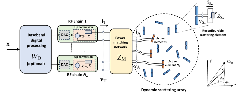
We consider the transmitting system illustrated in Fig. 1, where the DSA is composed of active antenna elements surrounded by a cloud of reconfigurable passive scatterers. The th element (active or passive) of the DSA, with , , is located in position . The th scatterer, with , is itself an antenna element terminated by a reconfigurable impedance load . To avoid power dispersion, we impose that the load is purely reactive, i.e., , where is the reconfigurable reactance.111From the technological point of view, the reconfigurable impedance load can be implemented using solutions similar to those applied for RISs such as PIN diodes and varactors [40]. Denote with the set of reconfigurable reactances and with the corresponding set of loads.
The DSA can be modeled as a linear -port network. The real-value bandpass voltage present at the generic port of the network is a modulated RF signal with carrier frequency and it can be represented as
| (1) |
where is the associated complex voltage envelope. Similarly, we define the complex envelope of the real-value bandpass current flowing into the port. Since the modulated signal carries information, then they have to be treated as random processes. The (average) active power delivered to the port is , where is the statistical expectation and the last equality holds thanks to the arbitrary constant in (1). We assume that the bandwidth of is sufficiently small such that the network properties are constant within and can be evaluated at the carrier frequency .
In a compact description, we define and the complex voltage and current envelopes (in the following denoted simply as voltages and currents) at the ports of the active antennas (i.e., the input ports of the DSA), and and the voltages and currents at the ports of the scatterers.222For notation convenience, in the following we omit the time dependence. We collect all the currents and voltages at the ports of the DSA in the vectors
| (6) |
All the interactions between the elements of the DSA are captured by the impedance matrix , which does not depend on the reconfigurable loads, and relates the voltages and currents of the ports as . In particular, the th element of represents the mutual coupling coefficient between the th and th elements obtained as the ratio between the open-circuit voltage observed at the th port and the excitation current applied to the th port supposing that the remaining ports are kept open (no current flow) [41]. It is convenient to divide the impedance matrix into the sub-matrices , , , and so that we can write
| (13) |
The voltages and currents at the input port of the DSA are related by the input impedance of the DSA as . By elaborating (13) and considering that at the scatterers’ ports it is , we obtain
| (14) |
which depends on parameters through the scatterers’ loads .
The active elements are connected to RF chains, including digital-to-analog converter (DAC) and up-conversion stages, through a -port power matching network whose purpose is to maximize the power transfer between the RF chains and the DSA. The relationship between the voltages and the currents present at the ports of the matching network is given by
| (19) |
where, assuming no losses in the power matching network, is equal to [39]
| (22) |
where is the output resistance of each RF chain. As it can be noticed from (22), the matching network depends on the DSA input impedance and hence on the parameters . Therefore, for a given DSA configuration, the matching network should be changed accordingly. This is possible using, for instance, adaptive matching networks [42]. In case a fixed network is employed instead, then not all the available power would be transferred to the DSA. With the power matching network, it turns out that , with and, assuming lossless antenna elements, the transmitted power corresponds to the radiated power given by
| (23) |
The reactive power can be evaluated as well as
| (24) |
from which the -factor of the system can be obtained as . The inverse of the -factor can be used as a rough estimate of the bandwidth of the DSA when [41].
We also foresee an optional baseband linear processing block implemented in the digital domain (digital precoder), described by the matrix , whose input is represented by the information vector to be transmitted. The matrix relates the transmitted information vector and the voltages at the input of the matching network, i.e., . In the following, we impose the arbitrarily normalization . Such a normalization ensures that , as typically considered in the signal processing community. The reconfigurable reactances along with the elements of matrix represent the set of parameters to be optimized to obtain the desired processing functionality, as will be described later.
By combining (25) and (28), we obtain a compact relationship between the information vector and the total current flowing in the DSA
| (29) |
where
| (32) |
accounts for the EM-level signal processing operated by the reconfigurable DSA as a function of the parameters .
Consider now test points located in positions , with , and that in each test point a conventional receiving antenna is used to receive the signal with gain . As commonly done in the literature, we assume that , , that is, the test points are located in the radiative region of the antenna structure and the receiving antennas do not affect the transmitting DSA. As an example, the set of antennas could represent a conventional receiving antenna array of a MIMO system. The useful component (i.e., without noise) of the received signal at the test positions is
| (33) |
where is the transimpedance matrix of the radio channel accounting for the propagation effects and is the end-to-end baseband equivalent channel matrix as commonly defined in signal processing.
III DSA with Hertzian Dipoles
To further develop our framework and derive some numerical examples from which obtaining important insights about the potential of DSAs, we suppose that all the antenna elements in the DSA, both active and scatterers, are modeled as Hertzian dipoles. In addition to making the derivation analytically tractable, the consideration of Hertzian dipoles can also be justified by the fact that the discrete infinitesimal dipole approximation is a flexible technique in computational electromagnetics for modeling and solving more complex antenna/scatterers structures [43].
Accordingly, we model the th dipole as a very short wire of length and radius , with and generic orientation , where and represent, respectively, the elevation angle and the angle with respect to axis , according to the reference coordinates system illustrated in Fig. 1. The th element of vector is the current present at the port of the th dipole.
The total current density distribution in the DSA is given by
| (34) |
Therefore, the EM field at the generic location excited by the current density in free space can be evaluated as [25]
| (35) |
where is the volume in which the current flows and is the Green’s dyadic given by [41]
| (36) |
with being the wave number and where we grouped the terms multiplying the factors , , and . By substituting (34) in (35), we obtain
| (37) |
The open-circuit voltage at the th dipole caused by the current of the th dipole by assuming all the other currents are equal to zero is
| (38) |
From (38), the generic element of the impedance matrix associated with the DSA can be easily obtained as
| (39) |
for . For , corresponds to the self-impedance of the Hertzian dipole which is given by [41]
| (40) |
In the free-space propagation condition, the channel transimpedance matrix in (33) can be easily derived. To elaborate, the electrical field intensity at the receiving test antenna located at can be computed once the currents , flowing into the dipoles (active and scatterers), are known
| (41) |
where is the polarization direction of the th receiving antenna. As a consequence, the received signal (assuming matched load and normalized to an impedance Ohm) is given by . Finally, the th element of the transimpedance matrix is given by
| (42) |
Since it is , (42) can be well approximated by neglecting the and components (reactive field) in (III) thus leading to
| (43) |
and
| (44) |
IV DSA Optimization
In this section, we illustrate a possible optimization strategy of the DSA along with its application to 3 different use cases. Numerical results associated with each use case will be reported in Sec. V.
IV-A Joint Optimization of the DSA and the Digital Precoder
For a given propagation scenario characterized by the transimpedance matrix and test points, suppose we fix a specification on the desired end-to-end channel matrix. The reconfigurable parameters of the DSA and the digital precoder can be obtained by solving the following constrained optimization problem:
| (45) | ||||
where the scalar accounts for the possible lack in the link budget to achieve that has to be eventually coped with increased transmitted power.
Unfortunately, in general, the constrained optimization problem in (45) is not convex thus making its numerical solution more challenging. A possible approach to translating it into an unconstrained optimization problem is to resort to the following alternate optimization procedure:
-
•
STEP 0: We set the candidate vector to an initial guess value, for instance randomly chosen or equal to zero.
-
•
STEP 1:
For a fixed , it is possible to find in closed form the values of and that minimize the objective function and satisfy the constraint in (45). In particular, we solve the following equation
(46) of which the minimum norm solution is
(47) The corresponding values of and are, therefore,
(48) and
(49) -
•
STEP 2:
Starting from the candidates and from STEP 1, the following unconstrained minimization problem involving only is solved numerically
(50) -
•
STEP 3: Repeat STEPS 1 and 2 for a given number iterations or until no significant variations of the parameters take place.
The inclusion of the digital precoder, while not strictly necessary, may aid in the optimization process of the DSA by handling a portion of the processing when . If omitted, we set , and only proceed with STEP 2 once. Of course, alternative optimization problems apart from (45) can also be considered, such as those involving the -factor as an optimization target or constraint. In many applications (e.g., beam steering, as seen in use case 1 below), the optimization process can be performed offline, computed once to create a dictionary of various DSA parameters for different steering directions of interest or, more broadly, different beam forms. In such cases, the complexity of the optimization algorithm is not a concern. However, in other scenarios, performing optimization offline may not be feasible, necessitating online optimization based, for example, on the channel state information (CSI). In this situation, developing efficient algorithms to minimize (50), potentially considering the structure of , becomes pertinent. This aspect exceeds the scope of this paper and is reserved for future investigations. In the numerical results, the standard numerical tool based on the quasi-Newton method [44] with iterations is utilized to minimize (50).
IV-B Use Case 1: Beam Forming
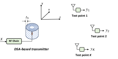
Suppose we want to design a single-input DSA (, no digital precoding) realizing a generic radiation diagram, for instance, imposing that at the test locations , the channel matrix , , assumes the desired value (see Fig. 2). For instance, one might define a uniform set of test points on the plane a distance in the far-field region of the DSA, with , and maximize the radiation diagram at the th direction (beam steering). This can be achieved by setting , for , and zero otherwise, being the desired received power. Incidentally, after the optimization process, the resulting parameter will represent the required transmitted power to satisfy the link budget. It is worth noticing that, in principle, only the optimization at the single test point , i.e., , would suffice to obtain the desired beam steering result. However, the addition of many other test points set to zero helps the minimization algorithm to speed up and avoid the convergence to bad local minima.
IV-C Use Case 2: Multi-user MISO
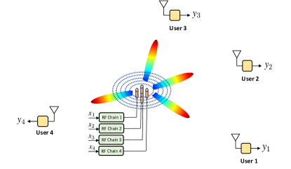
In this second use case, we consider a multi-user MISO downlink scenario shown in Fig. 3, where an DSA with RF chains (one per user) has to be designed to serve simultaneously single-antenna users located in generic positions , , by maximizing the signal-to-interference noise ratio (SINR) at each user according to the zero-forcing criterium [45]. Users can be both in the radiating near-field and far-field regions of the DSA.
Given the channel transimpedance matrix , where is the channel vector associated with the th user, the precoding matrix is , where is a normalization factor to make unitary, i.e., [45]. Therefore, the DSA and the digital precoder must be designed such that
| (51) |
leading to
| (52) |
This is equivalent to setting in the optimization problem in (45).
IV-D Use Case 3: Multi-layer MIMO Communication
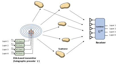
In this use case, we consider a MIMO communication with a receiving conventional uniform linear array (ULA) with elements spaced at illustrated in Fig. 4. The purpose is to design the DSA in such a way an optimal multi-layer MIMO link is established between the transmitter and the receiver. It is well known from MIMO theory that for a given generic propagation scenario with channel transimpedance matrix characterized by rank , up to parallel orthogonal links (layers) can be established between the transmitter and the receiver on which independent data stream can be transmitted [45]. To exploit all of them, it must be and the DSA must implement a suitable precoding strategy, i.e., act as an Holographic EM precoder.
Let us introduce the SVD of the channel transimpedance
| (53) |
where and contain the left and right eigenvectors, respectively, and is a diagonal matrix gathering the singular values of the channel transimpedance matrix . A typical MIMO setup, assuming the CSI is available at the transmitter, requires a precoding operation at the transmitter and a combining operation at the receiver such that the channel is diagonalized, i.e., the end-to-end channel matrix is proportional to the diagonal matrix . Assuming the receiver performs the combining operation , the MIMO channel is diagonalized if we design the DSA implementing the precoding by setting
| (54) |
or, equivalently,
| (55) |
In this manner, it results
| (56) |
and parallel communication layers can be established. The designed DSA implements the optimal precoding by using no more than RF chains (i.e., the minimum possible value) which is much simpler and less energy consuming than any conventional full digital or hybrid solution.
V Numerical Results
In this section, we present some numerical results related to the use cases described in Sec. IV with the purpose of validating and investigating the potential of the proposed DSA with respect to classical array structures. The following parameters have been considered in the numerical evaluations if not otherwise specified: GHz, dB, Ohm, , , , vertical polarization (, ).
V-A Beam Forming and Superdirectivity
We first investigate the beam forming capabilities of the DSA using one RF chain ( active antenna element) and the deployment of the scatterers according to concentric cylinders with incremental radius of step and scatterers separated of within each cylinder along the circle and the axis (see Fig. 2). We denote with the number of vertical rings composing each cylinder. The cylindric structure appears very appealing especially for its use in base stations or access points thanks to its circular symmetry. When , the cylinder degenerates into a disk. Obviously, other structures can be considered as well depending on the specific application.
The target end-to-end channel matrix with test points deployed on the plane at distance m (far field) according to the use case in Sec. IV-B was considered for 4 different steering angles, , , , and , respectively. Only the optimization Step 2 was performed with iterations and setting (in this case is a scalar and no digital processing takes place).
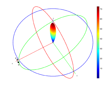
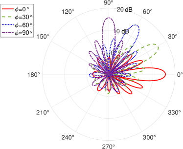
In Fig. 5, the radiation diagrams for the 4 steering angles obtained with , , (disk shape), corresponding to scatterers are shown. As it can be observed, the gain of the DSA is independent of the angle and it is about dB. In addition, limited back radiation is obtained without the need to insert a ground plane that would impede the steering in the angle range . An example of the corresponding 3D radiation diagram for steering angle is illustrated in Fig. 6.
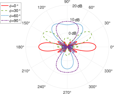
As pointed out in the Introduction, the performance of any SIM is constrained by the final layer surface of the structure, therefore it is upper bounded by that one can obtain by replacing the SIM with a full digital planar or linear array with the same layout and number of elements. Therefore, for the sake of comparison, we consider the radiation diagrams obtained using a standard full-digital ULA and a uniform circolar array (UCA) with the same aperture of the DSA (cm diameter) in the plane. The corresponding radiation diagrams are reported in Figs. 7 and 8, respectively. These arrays require and active antennas compared to only one active antenna of the DSA. As well-known, in ULAs the gain degrades when approaching from a maximum value of dB (about , with the gain of the Hertzian dipole) and symmetric back radiation is present. Instead, with the UCA the gain (dB) is insensitive to the steering direction at the expense of higher side lobes. Nevertheless, in both cases the proposed DSA exhibits superdirectivity capability with an additional gain of dB and dB, respectively. Contrarily to standard arrays, where superdirectivity is obtained only in the end-fire direction [19], here notably superdirectivity is equally obtained in all steering directions.
| Configuration | Gain (dB) | -factor | |
|---|---|---|---|
| , | 15 | 89 | 1.1 |
| , | 16.7 | 100 | 1.25 |
| , | 18.6 | 121 | 0.91 |
| , | 16 | 184 | 0.24 |
| , | 15.7 | 310 | 0.24 |
| , | 20.4 | 363 | 0.3 |
| 60 | 121 | 242 | 484 | |
|---|---|---|---|---|
| Gain (dB) | 12.3 | 17 | 18.8 | 18 |
| -factor | 0.29 | 1 | 1.55 | 3 |
In Table I, the impact of the cylinders spacing and the number of rings is investigated. As it can be noticed, the maximum gain is obtained for confirming that superdirectivity can be achieved only by exploiting the mutual coupling between the antenna elements but, at the same time, that there is an optimum spacing value to be found. In fact, on one hand, higher spacing reduces the coupling and hence the contribution to radiation of those scatterers located far away from the active element. On the other hand, very close spacing tightens the coupling between the elements and reduces the DoF available for optimization. A higher number of rings () further increases the directivity by thinning the radiation diagram in the direction. The corresponding -factor is in general relatively small denoting a wideband characteristic of the DSA under the considered setting and there is no need to generate very high currents as happens in conventional superdirective end-fire arrays [39].
An example using a random deployment of the scatterers within a disk as a function of their density is provided in Table II for a fixed diameter of cm. As it can be seen, the achievable performance is similar to that of the regular cylindrical deployment when compared with the same number of scatterers even though in general higher values of -factor are obtained because of the possibility that couples of scatterers are very close to each other. The analysis and optimization of scatterers deployment strategies is a topic that deserves future investigations.
An interesting aspect worth consideration is the sensitivity of the performance to parameter mismatch that might arise in practical implementations. We evaluated the gain degradation for the configuration in Fig. 5 when the actual implemented th parameter of the DSA, , is affected by an error modeled as a zero-mean Gaussian random variable with standard deviation , i.e., . The corresponding gains obtained for , and of the nominal absolute value are, respectively, dB, dB, and dB, showcasing a dB loss with a relative error.
V-B Multi-user MISO
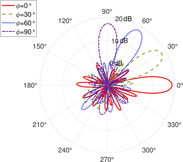
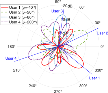
We consider now the scenario of use case in Sec. IV-C illustrated in Fig. 3, where a DSA with , , , , active antennas and RF chains is used to communicate simultaneously with single-antenna users located at a distance of m and angles , , , and in the plane. The DSA has been optimized according to (51) (zero forcing criterium) with and . The corresponding radiation diagrams are shown in Fig. 9. The coupling between users is impressive (dB) at the expense of increased leakage in unwanted directions and a reduction of the gain of some dBs compared to the pattern in Fig. 5 corresponding to a single user.
Alternatively, one could use the approach in use case 1 of Sec. IV-B to reduce the leakage in unwanted directions and increase the gain. However, our numerical investigations have revealed that the corresponding coupling between users would increase significantly. Therefore, the choice of the optimization method strongly depends on the specific application requirements in terms of gain versus coupling.
V-C Multi-layer MIMO
Finally, we consider the scenario of use case 3 in Sec. IV-D shown in Fig. 4, where a multi-layer MIMO link with a user located at m equipped with a standard ULA with elements spaced of has to be established in non-line-of-sight (NLOS) condition. The DSA is equipped with active antennas and RF chains to allow the transmission of up to 4 data streams (layers) according to channel characteristics. The simulated NLOS channel consists of 5 multi-paths caused by the reflection of 5 scatterers located at angles and distance m. The corresponding strongest singular values of the channel are , which has clearly rank . The DSA has the following parameters , , , and it is optimized according to the criterium in (54) with and .
In Table III, the resulting coefficients of the end-to-end channel is reported. The comparison between the diagonal and off-diagonal values indicates that the coupling between different layers is completely negligible, i.e., the channel is almost perfectly diagonalized. Compared to the singular values of the channel in , the diagonal elements of exhibit the same behavior with a loss of about dB that can be ascribed to the fact that the antenna is not ideal. The effect of implementation errors is reported in the bottom part of the table for and relative error standard deviation, respectively. It can be seen that the effect of implementation errors becomes no longer negligible (coupling above dB) with relative error.
| Perfect implementation | |||
| -41.6 | -177 | -190 | -175 |
| -170 | -48 | -185 | -170 |
| -183 | -184 | -49.7 | -182 |
| -164 | -166 | -180 | -52.3 |
| relative implementation error | |||
| -41.9 | -90.6 | -80 | -80.5 |
| -89 | -48.7 | -98.5 | -86.7 |
| -87 | -111 | -50 | -84.9 |
| -120 | -101 | -89.7 | -52.5 |
| relative implementation error | |||
| -47 | -56.7 | -59.4 | -62.2 |
| -66.6 | -48.3 | -61.6 | -65.3 |
| -67 | -61.4 | -52.4 | -64.9 |
| -57.2 | -74.7 | -62.8 | -55.3 |
VI Conclusion
In this paper, we have introduced the concept of the dynamic scattering array (DSA) as an appealing technology aimed at shifting part of the signal processing from the digital domain to the EM domain. This is achieved through the joint optimization of EM processing and radiation of active and reconfigurable scattering elements interacting in the reactive near field. We have shown that the DSA provides unprecedented flexibility in managing the EM field by reducing or circumventing digital processing at the baseband, thereby surpassing the flexibility offered by classical MIMO and recent SIM implementations. Consequently, the reduction in RF chains and digital processing facilitates the realization of energy-efficient, low-latency, and cost-effective holographic MIMO systems, then addressing the sustainability concerns of future wireless networks.
Although numerous implementation challenges must be addressed before DSAs can become a reality, such as the design of flexible reconfigurable scatterers, we hope that our promising theoretical results will inspire further research into technologies for the efficient implementation of DSAs as a key enabler of holographic MIMO within the ESIT paradigm.
Acknowledgment
This work was supported by the European Union under the Italian National Recovery and Resilience Plan (NRRP) of NextGeneration EU, partnership on “Telecommunications of the Future” (PE00000001 - program “RESTART”), and by the HORIZON-JU-SNS-2022-STREAM-B-01-03 6G-SHINE project (Grant Agreement No. 101095738).
References
- [1] A. Dang, S., B. O., Shihada, and et al., “What should 6G be?” Nature Electronics 3, vol. 20-29, 2020.
- [2] N. Gonzalez-Prelcic, M. F. Keskin, O. Kaltiokallio, M. Valkama, D. Dardari, X. Shen, Y. Shen, M. Bayraktar, and H. Wymeersch, “The integrated sensing and communication revolution for 6G: Vision, techniques, and applications,” Proceedings of the IEEE, pp. 1–16, 2024.
- [3] E. Björnson, L. Sanguinetti, H. Wymeersch, J. Hoydis, and T. L. Marzetta, “Massive MIMO is a reality - what is next?: Five promising research directions for antenna arrays,” Digital Signal Processing, 2019. [Online]. Available: http://www.sciencedirect.com/science/article/pii/S1051200419300776
- [4] E. Björnson, Y. C. Eldar, E. G. Larsson, A. Lozano, and H. V. Poor, “Twenty-five years of signal processing advances for multiantenna communications: From theory to mainstream technology,” IEEE Signal Processing Magazine, vol. 40, no. 4, pp. 107–117, 2023.
- [5] C. You, Y. Cai, Y. Liu, M. Di Renzo, T. M. Duman, A. Yener, and A. L. Swindlehurst, “Next Generation Advanced Transceiver Technologies for 6G,” arXiv e-prints, p. arXiv:2403.16458, Mar. 2024.
- [6] D. Dardari and N. Decarli, “Holographic communication using intelligent surfaces,” IEEE Communications Magazine, vol. 59, no. 6, pp. 35–41, June 2021.
- [7] M. Di Renzo, F. H. Danufane, and S. Tretyakov, “Communication models for reconfigurable intelligent surfaces: From surface electromagnetics to wireless networks optimization,” Proceedings of the IEEE, vol. 110, no. 9, pp. 1164–1209, 2022.
- [8] Z. Wang, J. Zhang, H. Du, W. E. I. Sha, B. Ai, D. Niyato, and M. Debbah, “Extremely large-scale MIMO: Fundamentals, challenges, solutions, and future directions,” IEEE Wireless Communications, pp. 1–9, 2023.
- [9] D. Dardari, “Communicating with large intelligent surfaces: Fundamental limits and models,” IEEE Journal on Selected Areas in Communications, vol. 38, no. 11, pp. 2526–2537, Nov 2020.
- [10] A. A. D’Amico and L. Sanguinetti, “Holographic MIMO Communications: What is the benefit of closely spaced antennas?” arXiv e-prints, p. arXiv:2307.13467, Jul. 2023.
- [11] T. Gong, P. Gavriilidis, R. Ji, C. Huang, G. C. Alexandropoulos, L. Wei, Z. Zhang, M. Debbah, H. V. Poor, and C. Yuen, “Holographic MIMO communications: Theoretical foundations, enabling technologies, and future directions,” IEEE Communications Surveys & Tutorials, vol. 26, no. 1, pp. 196–257, 2024.
- [12] S. Phang, M. T. Ivrla, G. Gradoni, S. C. Creagh, G. Tanner, and J. A. Nossek, “Near-field MIMO communication links,” IEEE Transactions on Circuits and Systems I: Regular Papers, vol. 65, no. 9, pp. 3027–3036, 2018.
- [13] N. Decarli and D. Dardari, “Communication modes with large intelligent surfaces in the near field,” IEEE Access, vol. 9, pp. 165 648–165 666, 2021.
- [14] Y. Liu, J. Xu, Z. Wang, X. Mu, and L. Hanzo, “Near-Field Communications: What Will Be Different?” arXiv e-prints, p. arXiv:2303.04003, Mar. 2023.
- [15] H. Zhang, N. Shlezinger, F. Guidi, D. Dardari, M. F. Imani, and Y. C. Eldar, “Beam focusing for near-field multiuser MIMO communications,” IEEE Transactions on Wireless Communications, vol. 21, no. 9, pp. 7476–7490, Sep. 2022.
- [16] H. Zhang, N. Shlezinger, F. Guidi, D. Dardari, and Y. C. Eldar, “6G wireless communications: From far-field beam steering to near-field beam focusing,” IEEE Communications Magazine, vol. 61, no. 4, pp. 72–77, April 2023.
- [17] G. Torcolacci, N. Decarli, and D. Dardari, “Holographic MIMO communications exploiting the orbital angular momentum,” IEEE Open Journal of the Communications Society, vol. 4, pp. 1452–1469, 2023.
- [18] A. S. Y. Poon and D. N. C. Tse, “Does superdirectivity increase the degrees of freedom in wireless channels?” in 2015 IEEE International Symposium on Information Theory (ISIT), 2015, pp. 1232–1236.
- [19] M. T. Ivrlac and J. A. Nossek, “The multiport communication theory,” IEEE Circuits and Systems Magazine, vol. 14, no. 3, pp. 27–44, 2014.
- [20] L. Han, H. Yin, and T. L. Marzetta, “Coupling matrix-based beamforming for superdirective antenna arrays,” in ICC 2022 - IEEE International Conference on Communications, 2022, pp. 5159–5164.
- [21] A. Alkhateeb, O. El Ayach, G. Leus, and R. W. Heath, “Channel estimation and hybrid precoding for millimeter wave cellular systems,” IEEE Journal of Selected Topics in Signal Processing, vol. 8, no. 5, pp. 831–846, 2014.
- [22] J. Zhu, Z. Wan, L. Dai, M. Debbah, and H. V. Poor, “Electromagnetic Information Theory: Fundamentals, Modeling, Applications, and Open Problems,” arXiv e-prints, p. arXiv:2212.02882, Dec. 2022.
- [23] M. D. Renzo and M. D. Migliore, “Electromagnetic signal and information theory,” IEEE BITS the Information Theory Magazine, pp. 1–13, 2024.
- [24] E. Björnson, C.-B. Chae, J. Heath, Robert W., T. L. Marzetta, A. Mezghani, L. Sanguinetti, F. Rusek, M. R. Castellanos, D. Jun, and Ö. Tugfe Demir, “Towards 6G MIMO: Massive Spatial Multiplexing, Dense Arrays, and Interplay Between Electromagnetics and Processing,” arXiv e-prints, p. arXiv:2401.02844, Jan. 2024.
- [25] D. Dardari, “Reconfigurable electromagnetic environments: A general framework,” IEEE Journal on Selected Areas in Communications, pp. 1–16, 2024.
- [26] A. Silva, F. Monticone, G. Castaldi, V. Galdi, A. Alù, and N. Engheta, “Performing mathematical operations with metamaterials,” Science, vol. 343, no. 6167, pp. 160–163, 2014. [Online]. Available: https://science.sciencemag.org/content/343/6167/160
- [27] J. An, C. Xu, D. W. K. Ng, G. C. Alexandropoulos, C. Huang, C. Yuen, and L. Hanzo, “Stacked intelligent metasurfaces for efficient holographic MIMO communications in 6G,” IEEE Journal on Selected Areas in Communications, vol. 41, no. 8, pp. 2380–2396, 2023.
- [28] D. Pozar, “Beam transmission of ultra short waves: An introduction to the classic paper by H. Yagi,” Proceedings of the IEEE, vol. 85, no. 11, pp. 1857–1863, 1997.
- [29] M. Faenzi, G. Minatti, D. González-Ovejero, F. Caminita, E. Martini, C. D. Giovampaola, and S. Maci, “Metasurface antennas: New models, applications and realizations,” Scientific Reports, vol. 9, no. 10178, pp. 1–14, 2019.
- [30] N. Shlezinger, G. C. Alexandropoulos, M. F. Imani, Y. C. Eldar, and D. R. Smith, “Dynamic metasurface antennas for 6G extreme massive MIMO communications,” IEEE Wireless Communications, vol. 28, no. 2, pp. 106–113, 2021.
- [31] K.-K. Wong, W. K. New, X. Hao, K.-F. Tong, and C.-B. Chae, “Fluid antenna system - Part I: Preliminaries,” IEEE Communications Letters, vol. 27, no. 8, pp. 1919–1923, 2023.
- [32] L. Pringle, P. Harms, S. Blalock, G. Kiesel, E. Kuster, P. Friederich, R. Prado, J. Morris, and G. Smith, “A reconfigurable aperture antenna based on switched links between electrically small metallic patches,” IEEE Transactions on Antennas and Propagation, vol. 52, no. 6, pp. 1434–1445, 2004.
- [33] D. Rodrigo, B. A. Cetiner, and L. Jofre, “Frequency, radiation pattern and polarization reconfigurable antenna using a parasitic pixel layer,” IEEE Transactions on Antennas and Propagation, vol. 62, no. 6, pp. 3422–3427, 2014.
- [34] N. U. Hassan, J. An, M. Di Renzo, M. Debbah, and C. Yuen, “Efficient beamforming and radiation pattern control using stacked intelligent metasurfaces,” IEEE Open Journal of the Communications Society, vol. 5, pp. 599–611, 2024.
- [35] J. An, M. Di Renzo, M. Debbah, H. V. Poor, and C. Yuen, “Stacked Intelligent Metasurfaces for Multiuser Downlink Beamforming in the Wave Domain,” arXiv e-prints, p. arXiv:2309.02687, Sep. 2023.
- [36] J. An, C. Yuen, M. Di Renzo, M. Debbah, H. V. Poor, and L. Hanzo, “Stacked Intelligent Metasurface Performs a 2D DFT in the Wave Domain for DOA Estimation,” arXiv e-prints, p. arXiv:2310.09861, Oct. 2023.
- [37] C. Liu, L. Ma, Q., Z.J., and et al., “Classification of metal handwritten digits based on microwave diffractive deep neural network,” Nat Electron, no. 5, pp. 113–122, 2022.
- [38] Z. Gu, Q. Ma, X. Gao, J. W. You, and T. J. Cui, “Classification of metal handwritten digits based on microwave diffractive deep neural network,” Advanced Optical Materials, vol. 12, no. 7, p. 2301938, 2024. [Online]. Available: https://onlinelibrary.wiley.com/doi/abs/10.1002/adom.202301938
- [39] M. T. Ivrlac and J. A. Nossek, “Toward a circuit theory of communication,” IEEE Transactions on Circuits and Systems I: Regular Papers, vol. 57, no. 7, pp. 1663–1683, 2010.
- [40] G. Alexandropoulos, D. Phan-Huy, K. Katsanos, and et al., “RIS-enabled smart wireless environments: deployment scenarios, network architecture, bandwidth and area of influence,” J Wireless Com Network, vol. 103, pp. 1–38, 2023.
- [41] C. A. Balanis, Antenna Theory: Analysis and Design. New Jersey, USA: Wiley, 2016.
- [42] Alibakhshikenari, M. Virdee, P. B.S. Shukla, and et al., “Improved adaptive impedance matching for RF front-end systems of wireless transceivers,” Sci Rep 10, no. 14065, pp. 1–11, 2020.
- [43] S. M. Mikki and A. A. Kishk, “Theory and applications of infinitesimal dipole models for computational electromagnetics,” IEEE Transactions on Antennas and Propagation, vol. 55, no. 5, pp. 1325–1337, 2007.
- [44] R. Fletcher, Practical Methods of Optimization - Vol. I. John Wiley and Sons, 1980.
- [45] D. Tse and P. Viswanath, Fundamentals of Wireless Communication. New York, NY: Cambridge University Press, 2005.