Peculiarities of the Landau level collapse on graphene ribbons in the crossed magnetic and in-plane electric fields

Abstract

Employing the low-energy effective theory alongside a combination of analytical and numerical techniques, we explore the Landau level collapse phenomenon, uncovering previously undisclosed features. We consider both finite-width graphene ribbons and semi-infinite geometries subjected to a perpendicular magnetic field and an in-plane electric field, applied perpendicular to both zigzag and armchair edges. In the semi-infinite geometry the hole (electron)-like Landau levels collapse as the ratio of electric and magnetic fields reaches the critical value $+(-)1$. On the other hand, the energies of the electron (hole)-like levels remain distinctive near the edge and deeply within the bulk approaching each other asymptotically for the same critical value. In the finite geometry, we show that the electron (hole)-like levels become denser and merge forming a band.

I Introduction

Rabi [1] was the one who solved the just-discovered Dirac equation for a free electron in a homogeneous magnetic field employing the symmetric gauge. Four months earlier, Fock [2] calculated the energy levels of a nonrelativistic electron subjected to both a magnetic field and a harmonic oscillator potential. However, he did not explore the limit in the absence of the potential, while the work of Rabi demonstrated the quantization of energy for free electrons. Frenkel and Bronstein [3] found quantized levels in the magnetic field now known as Landau levels independently of Landau himself [4]. In fact, the aim of a paper [3] was to investigate whether the discrete set of energy levels of free electrons constituted one of the paradoxes associated with the Dirac equation or corresponded to the real physical phenomenon which is not yet observed experimentally.

However, the experimental exploration of relativistic-like Landau levels, distinct from nonrelativistic counterparts, became attainable almost 80 years later in condensed matter systems, thanks to the groundbreaking discovery of graphene in 2005 [5, 6].

Furthermore, the fact that graphene is two-dimensional material allows to access the regime when the confining potential at the edges of graphene nanoribbons is atomically sharp. The quantum Hall edge states in this case are defined by boundary conditions of vanishing electron wave functions at the crystal edges.

It’s worth noting that conventional experiments conducted on two-dimensional semiconductors primarily access the regime characterized by electrostatically reconstructed edges. In this case, the system reduces its energy by reconfiguring the edge states into steps, which give rise to alternating compressible and incompressible stripes [7]. Additionally, visualizing these edge states is difficult because they are buried inside the semiconductors.

Graphene, therefore, offers an opportunity to investigate the real-space structure of edge states using scanning probe techniques [8, 9], while avoiding their electrostatic reconstruction. Other techniques of visualization of charge transport through Landau levels are also available [10, 11, 12].

Undoubtedly, the most captivating features arise from the relativistic Landau levels, which lack counterparts in standard electron systems. One notable phenomenon among them is the Landau level collapse in Ref. [13] (see also Ref. [14]) and subsequently observed experimentally in Refs. [15, 16].

For the massive Dirac with the dispersion, $\mathcal{E}(p)=\pm\sqrt{v_{F}^{2}p^{2}+\Delta^{2}}$, where $v_{F}$ is the Fermi velocity, $\Delta$ is the gap, the spectrum in the perpendicularly crossed magnetic, $H$, and electric, $E$, fields reads [17]

$$\begin{split}\mathcal{E}_{n}&=\mathcal{E}^{\ast}_{n}-\hbar k\frac{cE}{H},\\ \mathcal{E}^{\ast}_{n}&=\pm(1-\beta^{2})^{3/4}\sqrt{\frac{2n\hbar v_{F}^{2}eH}{c}+\frac{\Delta^{2}}{(1-\beta^{2})^{1/2}}},\end{split}$$ (1)

where $n=0,1,\ldots$, $k$ is the in-plane wave vector along the direction perpendicular to the electric field, $\beta=v_{0}/v_{F}=cE/(v_{F}H)$. Here and in what follows we assume that $H>0$ and use CGS units.

As the dimensionless parameter $\beta$ reaches its critical value, $|\beta_{c}|=1$, the Landau level staircase merges into one level [13, 14]. This collapse of the Landau levels can be regarded as a transition from the closed elliptic quasiparticle orbits for $|\beta|<1$ ($|v_{0}|<v_{F}$) to open hyperbolic orbits for $|\beta|>1$ ($|v_{0}|>v_{F}$) [18].

For $\Delta=0$, the spectrum Eqs. (1) reduces to the spectrum obtained in [13, 14]. The generalization for a finite $\Delta$ case was done in Ref. [17] (see also recent works [19, 20]).

The validity of long wavelength approximation for $\beta\neq 0$ was verified in Ref. [13] by performing numerical computations using the tight-binding model for graphene lattices of a finite size with the zigzag edges. It is stated in Ref. [13] that the Landau level collapse still occurs at the lower value of $\beta_{c}\simeq 0.9$. However, a careful examination of the corresponding figure from Ref. [13] reveals that this phenomenon does not manifest as a collapse in the same manner as in the case of an infinite system. Instead, it signifies an increase in the level density. As the levels approach one another, their finite width causes them to begin overlapping. In this context, the Landau level collapse does occur on the ribbon; however, its interpretation differs from that of the infinite system case.

Now we briefly overview the relevant literature. The evolution of edge states in the presence of an electric field was also explored by numerical computations conducted on a finite lattice in Refs. [21, 22].

Besides the analytical studies of Landau levels in crossed fields on an infinite plane [13, 14], the levels have also been explored for ribbons and semi-infinite geometries using the low-energy model without an electric field [23, 24, 25, 26, 27, 28, 29, 30].

To the best of our knowledge, the only analytic study of Landau levels in crossed magnetic and electric fields applied to ribbons was done in the recent work of the authors [31]. A special attention was paid to the analytical analysis of dispersionless surface modes localized at the zigzag edge.

The aim of this study is to complement the analysis presented in Ref. [31] by uncovering the undisclosed features of Landau level collapse in half-planes and ribbons with zigzag edges. Additionally, we broaden our investigation to include ribbons and half-planes with armchair edges. We point out that the very meaning of the Landau level collapse becomes different in the restricted geometry.

The paper is organized as follows. In Sec. II, we introduce a low-energy model for a graphene ribbon with zigzag and armchair edges subject to crossed magnetic and electric fields and represent the main equations in the unified form. General solutions of these equations in terms of the parabolic cylinder function are presented in Sec. III. The numerical and supporting analytical results in the half-plane geometry for the zigzag and armchair edges are described in Secs. IV (the details of the calculation are provided in Appendix A) and VI, respectively. A new property of the Landau level collapse, viz. that some levels do not collapse at the edge is considered in Secs. IV.2 and VI.2. The critical regime, $|\beta|=1$, is addressed in Sec. V, where the main results of this work are obtained. In Sec. VII the summary of the obtained results is given. Moreover, the Supplemental Material (SM) [32] presents additional calculations useful for comparison with the results given in the main text.

II Model

To determine eigenenergy $\mathcal{E}$ we consider the stationary Dirac equation, $H\Psi(\mathbf{r})=\mathcal{E}\Psi(\mathbf{r})$, with the Hamiltonian describing low-energy excitations in graphene:

$$H=\hbar v_{F}\left(-\alpha_{1}iD_{x}-\alpha_{2}iD_{y}\right)+\Delta\alpha_{3}+V(\mathbf{r}).$$ (2)

Here the $4\times 4$ $\alpha$-matrices $\alpha_{i}=\tau_{3}\otimes\sigma_{i}$ and the Pauli matrices $\tau_{i}$, $\sigma_{i}$ (as well as the $2\times 2$ unit matrices $\tau_{0}$, $\sigma_{0}$) act on the valley ($\mathbf{K}_{\eta}$ with $\eta=\pm$) and sublattice ($A,B$) indices, respectively, of the four-component spinors $\Psi^{T}=\left(\Psi_{+}^{T},\Psi_{-}^{T}\right)=\left(\psi_{AK_{+}},\psi_{BK_{+}},\psi_{BK_{-}},\psi_{AK_{-}}\right)$. This representation is derived from a tight-binding model for graphene (see, e.g., Ref. [33]) and thus allows for the formulation of appropriate boundary conditions for armchair and zigzag edges in the continuum model. We investigate both massless Dirac-Weyl fermions in pristine graphene and massive Dirac fermions with a mass (gap) parameterized as $\Delta$

The gap $\Delta$ considered in the present work corresponds to the time-reversal symmetry conserving gap $\tilde{\Delta}$ in the notation of [27, 28, 29] and is related to the carrier density imbalance between the A and B sublattices. Recall that this gap can be introduced in graphene when it is placed on top of hexagonal boron nitride (G/hBN) and the crystallographic axes of graphene and hBN are aligned.

The orbital effect of a perpendicular magnetic field $\mathbf{H}=\nabla\times\mathbf{A}$ is included via the covariant spatial derivative $D_{j}=\partial_{j}+(ie/\hbar c)A_{j}$ with $j=x,y$ and $-e<0$, while the potential $V(\mathbf{r})$ corresponds to the static electric field $e\mathbf{E}=\nabla V(\mathbf{r})$. The Zeeman interaction is neglected in this paper, because of its smallness for moderate values of magnetic field (see, e.g., Ref. [33]).

We consider the ribbons with the armchair and zigzag edges as shown in Fig. 1 (a) and (b), respectively.

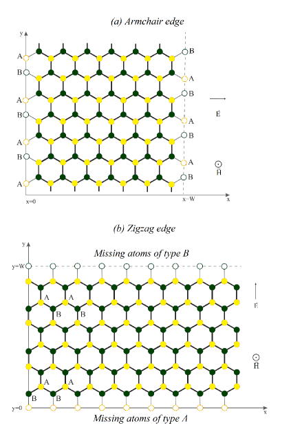
Figure 1: The lattice structure of a finite width graphene ribbon with (a) armchair and (b) zigzag edges.

The ribbons are subjected to a combination of crossed uniform magnetic and electric fields. The magnetic field $\mathbf{H}$ is applied perpendicular to the plane of the graphene ribbon along the positive $z$ axis, while the in-plane electric field $\mathbf{E}$ is applied perpendicular to the ribbon edges.

As we will discuss below, only the boundary conditions for the armchair edges (8) involve an admixture of the wave-functions from both $\mathbf{K}_{\eta}$ points, while the equation (2) splits into a pair of two independent Dirac equations for each $\mathbf{K}_{\eta}$ point, $H_{\eta}\Psi_{\eta}(\mathbf{r})=\mathcal{E}\Psi_{\eta}(\mathbf{r})$ with the Hamiltonian

$$H_{\eta}=-i\hbar v_{F}\eta(\sigma_{1}D_{x}+\sigma_{2}D_{y})+\eta\Delta\sigma_{3}+V(\mathbf{r}).$$ (3)

One can see from Eq. (3) that having the solutions for $\mathbf{K}_{+}$ point, the corresponding solutions for $\mathbf{K}_{-}$ can be obtained by changing the signs of energy $\mathcal{E}$ and electric field in $V(\mathbf{r})$. Finally, one should take into account that for the spinor $\Psi_{-}$ the components of the spinor corresponding to $A$ and $B$ sublattices are exchanged as compared to $\Psi_{+}$.

II.1 Armchair edge

An armchair edge is parallel to the $y$ as shown in Fig. 1 (a). The in-plane electric field $\mathbf{E}$ is applied respectively in $x$ direction, so the potential $V(\mathbf{r})=eEx$. In this case, it is convenient to consider the magnetic field $H$ in the following Landau gauge $(A_{x},A_{y})=(0,Hx)$, where $H$ is the magnitude of a constant magnetic field orthogonal to the graphene plane.

Accordingly, the differential equations in Eq. (2) do not depend explicitly on the $y$-coordinate. Therefore, the wave functions are plane waves in the $y$-direction,

$$\negthickspace\negthickspace\psi_{\scriptscriptstyle{AK_{\pm}}}(\mathbf{r},k)=\frac{e^{iky}}{\sqrt{2\pi l}}u_{\scriptscriptstyle{\pm}}(x,k),\thickspace\psi_{\scriptscriptstyle{BK_{\pm}}}(\mathbf{r},k)=\frac{e^{iky}}{\sqrt{2\pi l}}v_{\scriptscriptstyle{\pm}}(x,k),$$ (4)

where $l=\sqrt{\hbar c/|eH|}$ is the magnetic length. The wave vector $k$ measures the displacement from $\mathbf{K}_{\eta}$ points. A specific choice of the coordinate system in Ref. [33] defines $\mathbf{K}{\pm}=\pm(2\pi/a),(2/3,0)$, where $a$ is the lattice constant. The maximum value of the wave vector $k$ is constrained by the boundaries of the first Brillouin zone.

Recall that the wave vector $k$ determines the center of the electron orbital along the $x$ direction, given by $x_{k}=-kl^{2}$. For a system with a ribbon of finite width $W$, such as $0\leq x\leq W$, the condition that the peak of the wave function lies within the ribbon is met only for eigenstates with wave vectors $k$ in the finite range $-W/l^{2}\leq k\leq 0$. This phenomenon is known as the position-wave vector duality in the Landau gauge.

Substituting Eq. (4) in Eq. (2) we obtain the following system of equations for $\mathbf{K}_{+}$ point

$$\begin{pmatrix}\frac{eEx-\mathcal{E}+\Delta}{\hbar v_{F}}&-i\partial_{x}-ik-i\frac{e}{\hbar c}Hx\\ -i\partial_{x}+ik+i\frac{e}{\hbar c}Hx&\frac{eEx-\mathcal{E}-\Delta}{\hbar v_{F}}\end{pmatrix}\psi_{+}=0,$$ (5)

where the spinor ${\psi}_{+}^{T}=(u_{+},v_{+})$. One can see that the envelope functions $u_{+}(x,k)$ and $v_{+}(x,k)$ ($u_{-}(x,k)$ and $v_{-}(x,k)$) depend only on a single dimensionless combination of the variables, $\xi=x/l+kl$, so Eq. (5) acquires the form

$$\begin{pmatrix}\beta\xi-\varepsilon+\delta&-i\partial_{\xi}-i\xi\\ -i\partial_{\xi}+i\xi&\beta\xi-\varepsilon-\delta\end{pmatrix}\psi_{+}=0.$$ (6)

Here we introduced the notations for dimensionless quantities

$$\beta=\frac{cE}{v_{F}H},\quad\varepsilon=\frac{l\mathcal{E}}{\hbar v_{F}}+\beta kl,\qquad\delta=\frac{l\Delta}{\hbar v_{F}}.$$ (7)

The important dimensionless parameter $\beta$ in Eq. (7) describes the strength of the electric field relative to the magnetic field. In this paper, we restrict our analysis to the case where $|\beta|\leq 1$ and do not consider the pair creation regime.

To obtain the energy spectrum we need to supplement the differential equations for the envelope functions $u_{\pm}(x,k)$ and $v_{\pm}(x,k)$ functions with suitable boundary conditions. Such conditions can be derived from the tight-binding model [34, 35, 23, 24]. Note that in the tight-binding calculation the values of the total wave vector projected on the armchair edge direction coincide for the different $\mathbf{K}_{\eta}$ valleys (see e.g. Ref. [30]). This leads to valley admixing by the boundary condition:

$$x=0:\qquad\quad u_{+}(kl)+u_{-}(kl)=0,$$

$$v_{+}(kl)+v_{-}(kl)=0,$$ (8a)

$$x=W:\qquad\quad u_{+}(W/l+kl)+u_{-}(W/l+kl)=0,$$

$$v_{+}(W/l+kl)+v_{-}(W/l+kl)=0,$$ (8b)

see Fig. 1. As we shall see in Sec. VI, this choice of boundary conditions proves particularly convenient when transitioning from the ribbon configuration to the semi-infinite, half-plane geometry with $W\to\infty$. To consider the symmetry properties of the corresponding solutions it is more convenient to choose the ribbon centered at $y=0$, viz. $-W/2\leq x\leq W/2$. This case is briefly discussed in Sec. S3 of SM [32] in parallel to the consideration made for the zigzag edge case in Sec. S2.

II.2 Zigzag edge

A zigzag edge is parallel to the $x$ direction as shown in Fig. 1 (b). The in-plane electric field $\mathbf{E}$ is applied in $y$ direction, so the potential $V(\mathbf{r})=eEy$. In this case, it is convenient to consider the magnetic field $H$ in the following Landau gauge, $(A_{x},A_{y})=(-Hy,0)$.

Accordingly, the differential equations in Eq. (2) do not depend explicitly on the $x$-coordinate. Therefore, the wave functions are plane waves in the $x$-direction,

$$\negthickspace\negthickspace\psi_{\scriptscriptstyle{AK_{\pm}}}(\mathbf{r},k)=\frac{e^{-ikx}}{\sqrt{2\pi l}}u_{\scriptscriptstyle{\pm}}(y,k),\thickspace\psi_{\scriptscriptstyle{BK_{\pm}}}(\mathbf{r},k)=\frac{e^{-ikx}}{\sqrt{2\pi l}}v_{\scriptscriptstyle{\pm}}(y,k).$$ (9)

The center of the electron orbital along the $y$ direction is $y_{k}=-kl^{2}$. Since $0\leq y\leq W$, the wave vectors $k$ are within the range $-W/l^{2}\leq k\leq 0$. Note that the values of the total wave vector for the different $\mathbf{K}_{\eta}$ valleys in the tight-binding calculation fall in the different wave vectors domains, because $K_{+x}\neq K_{-x}$.

Substituting Eq. (9) in Eq. (3) we obtain the following system of equations for $\mathbf{K}_{+}$ point

$$\begin{pmatrix}\frac{eEy-\mathcal{E}+\Delta}{\hbar v_{F}}&-\partial_{y}-k-\frac{e}{\hbar c}Hy\\ \partial_{y}-k-\frac{e}{\hbar c}Hy&\frac{eEy-\mathcal{E}-\Delta}{\hbar v_{F}}\end{pmatrix}\psi_{+}=0,$$ (10)

where $\psi_{+}^{T}=(u_{+},v_{+})$. One can see that the envelope functions $u_{+}(y,k)$ and $v_{+}(y,k)$ ($u_{-}(y,k)$ and $v_{-}(y,k)$) depend only on a single dimensionless combination of the variables, $\xi=y/l+kl$. Finally, one can rewrite Eq. (10) in exactly the same form as Eq. (6), but for the spinor ${\tilde{\psi}}_{+}^{T}=(u_{+},-iv_{+})$ (see Ref. [31]). The notation, ${\tilde{\psi}}$, together with the opposite sign in $\exp(-ikx)$ as compared to [27, 28, 29] allows us to unify the equations describing zigzag and armchair edges.

To obtain the energy spectrum we need to supplement the differential equations for the envelope functions $u_{\pm}(y,k)$ and $v_{\pm}(y,k)$ functions with suitable boundary conditions. Such conditions can be derived from the tight-binding model [34, 35, 23, 24].

In the case of a graphene ribbon of a finite width in the $y$ direction, $0\leq y\leq W$, and with two zigzag edges parallel to the $x$ direction, the $A$ and $B$ components of wave functions should vanish on the opposite edges:

$$y =0:\qquad\quad u_{+}(kl)=u_{-}(kl)=0,$$ (11a)

$$y =W:\qquad v_{+}(W/l+kl)=v_{-}(W/l+kl)=0,$$ (11b)

see Fig. 1. As for the armchair edges, this choice of boundary conditions proves particularly convenient when transition is carried out from the ribbon configuration to the semi-infinite, half-plane geometry, with $W\to\infty$. To consider the symmetry properties of the corresponding solutions it is more convenient to choose the ribbon centered at $y=0$, viz. $-W/2\leq y\leq W/2$. This case is studied in Sec. S2 of SM [32].

III General solutions

As mentioned in Introduction, the Dirac equation (3) for the massless case, $\Delta=0$, and infinite plane was solved in Refs. [13, 14]. Here, we employ a different analytic approach [31] to investigate a finite system. The main equation (6) describing both zigzag and armchair cases can be rewritten in the following form

$$\partial_{\xi}\tilde{\chi}_{+}(\xi)=\left(\tilde{A}+\tilde{B}\xi\right)\tilde{\chi}_{+}(\xi),$$ (12)

where the $2\times 2$ $\xi$-independent matrices $\tilde{A},\tilde{B}$ are, respectively,

$$\tilde{A}=\begin{pmatrix}0&i(\varepsilon+\delta)\\ i(\varepsilon-\delta)&0\end{pmatrix},\quad\tilde{B}=\begin{pmatrix}1&-i\beta\\ -i\beta&-1\end{pmatrix},$$ (13)

and the spinor $\tilde{\chi}_{+}$ is either ${\tilde{\psi}}_{+}$ defined below Eq. (10) for the zigzag edge case or ${\psi}_{+}$ defined below Eq. (5) for the armchair edge case.

Whereas the problem with the radial electric field [20], which involves three matrices ${\hat{A}}/\rho+{\hat{B}}+{\hat{C}}\rho$ with $\rho$ being the radial variable, cannot be solved analytically, the present problem in the crossed uniform fields in the Cartesian coordinates is exactly solvable by diagonalizing the matrix $\tilde{B}$ as discussed in detail in [31]. Thus here we proceed directly to the general solution for the components of the spinor ${\tilde{\chi}}_{+}$:

$${\tilde{\chi}}_{+1}(\zeta) =iC_{+1}\left[\gamma U\left(a-1,\sqrt{2}\zeta\right)-\kappa_{+}U\left(a,\sqrt{2}\zeta\right)\right]$$ (14)

$$+iC_{+2} \left[\gamma V\left(a-1,\sqrt{2}\zeta\right)+\frac{\kappa_{+}}{a-1/2}V\left(a,\sqrt{2}\zeta\right)\right],$$

$${\tilde{\chi}}_{+2}(\zeta) =C_{+1}\left[U\left(a-1,\sqrt{2}\zeta\right)-\gamma\kappa_{+}U\left(a,\sqrt{2}\zeta\right)\right]$$ (15)

$$+C_{+2} \left[V\left(a-1,\sqrt{2}\zeta\right)+\frac{\gamma\kappa_{+}}{a-1/2}V\left(a,\sqrt{2}\zeta\right)\right].$$

Here the solutions are written in terms of the parabolic cylinder (Weber) functions $U(a,x)$ and $V(a,x)$ depend on the variable

$$\zeta=(1-\beta^{2})^{1/4}\xi+\frac{\beta\varepsilon}{(1-\beta^{2})^{3/4}}$$ (16)

with $\xi=y/l+kl$ either $\xi=x/l+kl$ for zigzag or armchair edges, the integration constants $C_{+1,+2}$ have the restored valley index $+$, and the following notations are introduced

$$\gamma=\frac{\beta}{1+\sqrt{1-\beta^{2}}},\qquad\kappa_{\pm}=\frac{\delta\sqrt{1-\beta^{2}}\pm\varepsilon}{\sqrt{2}(1-\beta^{2})^{3/4}},$$ (17)

$$a=\frac{1+2\kappa_{-}\kappa_{+}}{2}=\frac{1}{2}+\frac{\delta^{2}(1-\beta^{2})-\varepsilon^{2}}{2(1-\beta^{2})^{3/2}}.$$ (18)

The centers of the electron orbital can be defined by the condition $\zeta=0$, viz.

$$y_{k}=-kl^{2}-\frac{\beta l\varepsilon}{1-\beta^{2}}.$$ (19)

The particular relationship between $y_{k}$ and $\beta$ arises from the dependence of energy $\varepsilon$ on $\beta$. Substituting the spectrum (1) (see also Eq. (S4) in SM [32]) in the last equation one can see that for an infinite system

$$y_{k}=-kl^{2}-\frac{\beta l\mbox{sgn}\,(\varepsilon_{n})\sqrt{2n(1-\beta^{2})^{1/2}+\delta^{2}}}{(1-\beta^{2})^{1/2}}.$$ (20)

This illustrates that the electron and hole orbits become open on the opposite sides as $|\beta|\to 1$.

The derivation of the spectrum (1) for an infinite system, which utilizes the specific asymptotic behavior of the Weber parabolic cylinder functions, is included in Sec. S1 of the Supplementary Material (SM) [32] for completeness. We also included there in Secs. S2 and S3 the results for spectra of the ribbons with the zigzag and armchair edges, respectively. The symmetry relations (S11) and (S15) for the energy spectra of these ribbons are also provided. Our numerical results support an observation made in Introduction on the base of Ref. [13] and illustrate that the electron-like levels seem to be denser near $-kl\approx W/l$ edge, while the hole-like are denser for $kl\approx 0$.

To study the level behavior by analytic methods we simplify the problem by considering the semi-infinite geometry in Sec. IV. In particular, this enables us to investigate the specific of the Landau level collapse in the restricted geometry.

IV Half-plane with the zigzag edge

On a half-plane, normalizable wave functions can be expressed solely in terms of the function $U(a,x)$, which, as mentioned above, decays exponentially as $x\to\infty$. On the other hand, the function $V(a,z)$ grows exponentially in both directions as $x\to\pm\infty$ (see Refs. [32, 31]). This enables one to set $C_{+2}=0$ in the solutions (14) and (15) the $\mathbf{K}_{+}$ valley. However, unlike the case of an infinite plane, on a half-plane, there is no restriction on the parameter $a$ being a negative half-integer.

The zigzag boundary condition (11b) at $y=W\to\infty$ is naturally fulfilled as a consequence of the asymptotic behavior of $U(a,x\to\infty)$. The remaining boundary condition (11a) at $y=0$ leads to the requirement that the term with $C_{+1}$ in Eq. (14) must be zero. The latter condition results in the following equation for the spectrum for the $\mathbf{K}_{+}$ valley:

$$\gamma U\left(a-1,\sqrt{2}\zeta(0)\right)-\kappa_{+}U\left(a,\sqrt{2}\zeta(0)\right)=0.$$ (21)

Here $\zeta(0)=(1-\beta^{2})^{1/4}kl+\beta\varepsilon(1-\beta^{2})^{-3/4}$. Using the asymptotics Eq. (S1) from [32] one can verify that Eq. (21) also follows from the equation (S5) for the spectrum on the ribbon in the limit $W\to\infty$.

Similarly, for the $\mathbf{K}_{-}$ valley, the boundary condition (11a) at $y=0$ leads to the following equation:

$$U\left(a-1,\sqrt{2}\zeta(0)\right)+\gamma\kappa_{-}U\left(a,\sqrt{2}\zeta(0)\right)=0.$$ (22)

Eqs. (21) and (22) determine dimensionless energies $\varepsilon_{\alpha}=\varepsilon_{n}(kl)$ as functions of quantum numbers $\alpha\equiv(n,k)$. The corresponding spectra are computed numerically and presented for the gapless and gapped cases in Figs. 2 and 3, respectively. Notice that, unlike the figures in SM [32], we present the dimensionless energy $\varepsilon(k)$ herein. In contrast to the energy $\mathcal{E}$, this representation excludes the linear in $k$ part. This enables a clearer presentation of the results when considering higher values of $\beta$.

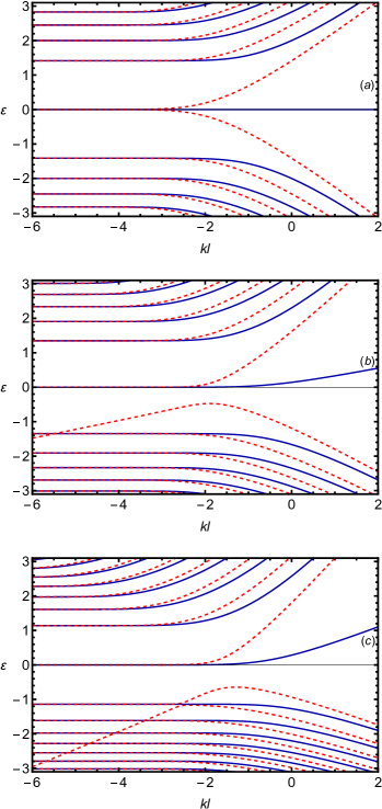
Figure 2: The energy spectra $\varepsilon(k)$ of the first few Landau levels near the zigzag edge of graphene’s half-plane for the gapless, $\Delta=0$ case. The solutions for the $\mathbf{K}_{+}$ and $\mathbf{K}_{-}$ valleys are shown by the solid (blue) and dashed (red) lines, respectively. (a) $\beta=0$; (b) $\beta=0.25$; (c) $\beta=0.5$

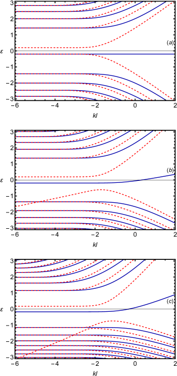
Figure 3: The energy spectra $\varepsilon(k)$ of the first few Landau levels near the zigzag edge of graphene for the gapped, $\delta=0.2$ case. The panels (a), (b) and (c) are for the same values of $\beta$ as in Fig. 2.

In contrast to Figs. S1 and S2 where we showed the $\mathbf{K}_{+}$ and $\mathbf{K}_{-}$ valleys on separate panels, here we superimpose both valleys on the same panel to allow a direct comparison of the corresponding energy levels. This is possible, because in the continuum model the wave vector $k$ is counted from $K_{\pm x}$ values. The negative values of $k$ correspond to the bulk, while the edge is at $k=0$.

Since a half-plane geometry is considered, for a finite $\beta$ the energies $\varepsilon(k)$ tend to the constant values in the bulk as $kl\to-\infty$. The presence of the edge at $y=W$ modifies this behavior: the hole-like levels including the blue line (the $\mathbf{K}_{+}$ solution) that goes to zero for $kl\to-\infty$ would go downward, while the electron-like levels go upward. Furthermore, the degeneracy of the solutions for the $\mathbf{K}_{+}$ and $\mathbf{K}_{-}$ valleys would be lifted near the other edge as one can see in Figs. S1 and S2.

The sole dispersive curve for $kl\to-\infty$, given that $\varepsilon(k)$ is considered, corresponds to the dispersionless state observed in the full spectrum $l\mathcal{E}(k)/(\hbar v_{F})$, viz. to the zero-energy lower branch of the $\mathbf{K}_{-}$ valley spectrum in the ribbon geometry. It describes the surface states mentioned in Sec. S2 A. The second edge of the ribbon supports a second dispersionless mode which is absent in a half-plane geometry. The surface state in the semi-infinite geometry is briefly discussed in Sec. IV.3. The analytical consideration of the Landau level spectrum in zero electric field was presented in [31] (see also [25]). Since for $E=0$ the presented below expressions reduce to the corresponding formulas from Ref. [31], we include them in Sec. S4 of SM [32] for a reference.

IV.1 Landau levels in the bulk for $\beta\neq 0$

It is possible to obtain the approximate analytic expressions that generalize Eqs. (S17) and (S18) from [32] in the bulk, viz. for $y_{0}=-kl^{2}\gg l$ or $kl\to-\infty$. The $\mathbf{K}_{+}$ valley solutions are

$$\varepsilon_{+,0}=-\delta\left(1-\beta^{2}\right)^{\frac{1}{2}}+\frac{\gamma\left(1-\beta^{2}\right)^{\frac{3}{4}}}{\sqrt{\pi}}e^{-\left(1-\beta^{2}\right)^{\frac{1}{2}}(kl)^{2}}$$ (23)

and

$$\begin{split}&\varepsilon_{+,n}^{2}-\delta^{2}\left(1-\beta^{2}\right)=2n\left(1-\beta^{2}\right)^{\frac{3}{2}}\left[1+\frac{2^{n}(kl)^{2n}}{\sqrt{\pi}n!}\right.\\ &\times\left.\frac{\gamma\left(1-\beta^{2}\right)^{\frac{2n+1}{4}}}{\sqrt{2n\left(1-\beta^{2}\right)^{\frac{1}{2}}+\delta^{2}}+\delta}e^{-\left(1-\beta^{2}\right)^{\frac{1}{2}}(kl)^{2}}\right]\end{split}$$ (24)

with $n=1,2,\ldots$. The corresponding solutions for $\mathbf{K}_{-}$ valley are

$$\varepsilon_{-,0}=\delta\left(1-\beta^{2}\right)^{\frac{1}{2}}+\frac{\left(1-\beta^{2}\right)^{\frac{3}{4}}}{\sqrt{\pi}\gamma}e^{-\left(1-\beta^{2}\right)^{\frac{1}{2}}(kl)^{2}}$$ (25)

and

$$\begin{split}&\varepsilon_{-,n}^{2}-\delta^{2}\left(1-\beta^{2}\right)=2n\left(1-\beta^{2}\right)^{\frac{3}{2}}\left[1+\frac{2^{n}(kl)^{2n}}{\sqrt{\pi}\gamma n!}\right.\\ \times&\left.\frac{\left(1-\beta^{2}\right)^{\frac{2n+1}{4}}}{\sqrt{2n\left(1-\beta^{2}\right)^{\frac{1}{2}}+\delta^{2}}-\delta}e^{-\left(1-\beta^{2}\right)^{\frac{1}{2}}(kl)^{2}}\right]\end{split}$$ (26)

with $n=1,2,\ldots$.

Note that since $\beta\neq 0$ in the derivation of the asymptotic (23), (24), (25) and (26), we have taken into account the contribution of another parabolic cylinder function in Eqs. (21) and (22) as compared to the solution of Eqs. (S16) from [32]. Thus, Eqs. (24) and (23) are valid for any value of $\beta\in]-1,1[$.

On the contrary, the contribution of $\gamma\kappa_{-}U(a,\sqrt{2}\zeta(0))$ in the equation (22) for the $\mathbf{K}_{-}$ valley spectrum leads to cancelation of a correction of the order $\sim\left(y_{0}/l\right)^{2n+1}e^{-\left(1-\beta^{2}\right)^{\frac{1}{2}}y_{0}^{2}/l^{2}}$, and hence, the correction of the lower order survives in Eq. (39), $\sim\gamma^{-1}\left(y_{0}/l\right)^{2n}e^{-\left(1-\beta^{2}\right)^{\frac{1}{2}}y_{0}^{2}/l^{2}}$. Therefore, in the case of the $\mathbf{K}_{-}$ valley, the limit $\beta\rightarrow 0$ in Eq. (26) [and Eq. (25)] is not applicable, hence it is valid for values of $\beta\in]-1,-\epsilon]\cup[\epsilon,1[$ with $\epsilon>0$.

IV.2 Landau levels at the edges for $\beta\neq 0$

We begin by presenting in Fig. 4 numerical solutions of Eqs. (21) and (22) for the energy spectra at the zigzag edge, $\varepsilon(kl=0)$, and $\delta=0$. These solutions are depicted as functions of $-1\leq\beta\leq 1$ for the first few Landau levels.

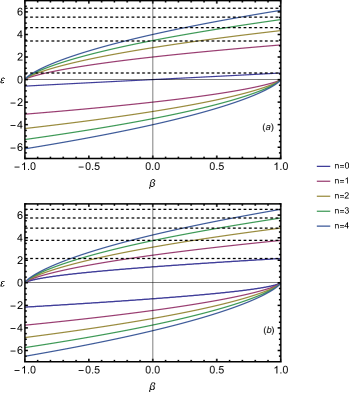
Figure 4: The energy spectra $\varepsilon(kl=0)$ at the zigzag edge versus electric field in terms of $\beta=cE/(v_{F}H)$ for $\delta=0$ for first few Landau levels. The dashed lines correspond to the energies given by Eq. (29): (a) For $\mathbf{K}_{+}$ valley, (b) For $\mathbf{K}_{-}$ valley.

For $\beta=0$ the values of the energies agree with the lower lines of Eqs. (S17) and (S18) from [32]. One can see that for the $\mathbf{K}_{+}$ valley the $n=0$ level does not collapse, while for the $n\neq 0$ levels the electron-like solutions with $\varepsilon>0$ merge to one point and collapse only when $\beta\to-1$. For $\beta\to 1$ the level energies tend to the different values and thus the electron-like levels do not collapse at the edge. On the contrary, the hole-like solutions with $\varepsilon<0$ merge and collapse for $\beta\to 1$, while for $\beta\to-1$ these levels do not collapse. For the $\mathbf{K}_{-}$ valley all $n\geq 0$ levels behave similarly to $n\neq 0$ levels in the $\mathbf{K}_{+}$ valley. We verified that the same behavior exhibits the spectra for finite values of $\delta$.

The observed behavior can be explained qualitatively using Eq. (19) for the centers of the electron orbital. Indeed, the Landau level collapse occurs when the corresponding center of electron or hole orbit remains in the bulk ($y>0$), while $y_{k}\to\infty$. The behavior of the levels on the opposite edge is interchanged when compared to the edge considered in this section, because in this case the bulk is for $y<0$.

Now we proceed to the discussion of the analytical results obtained for Eqs. (21) and (22) in the limit $kl\to 0$. Finding a straightforward generalization of solutions (S17) and (S18) from [32] near the edges, specifically when $y_{0}\ll l$ or $kl\to 0$, proves to be challenging. Nevertheless, it is possible to consider analytically two limiting cases: $|\beta|\ll 1$ and $|\beta|\rightarrow 1$. The details of the derivation are described in Appendix A, where we obtain that for $|\beta|\ll 1$ the solutions for the $\mathbf{K}_{\pm}$ valleys read, respectively,

$$\varepsilon_{+,0} =-\delta+\frac{1}{\sqrt{\pi}}\beta+o(\beta)$$ (27)

$$\varepsilon_{+,n} =\pm\sqrt{4n+\delta^{2}}\left[1+\frac{\Gamma\left(n+\frac{1}{2}\right)}{\Gamma\left(n\right)}\frac{2}{\pi\left(4n+\delta^{2}\right)}\right.$$

$$\times\left.\left(\frac{1}{\delta\pm\sqrt{4n+\delta^{2}}}\pm 2\sqrt{4n+\delta^{2}}\right)\beta+o(\beta)\right]$$

with $n=1,2,\ldots$, and

$$\begin{split}\varepsilon_{-,n}&=\pm\sqrt{2(2n+1)+\delta^{2}}\left[1-\frac{\Gamma\left(n+\frac{3}{2}\right)}{\Gamma\left(n+1\right)}\right.\\ &\times\frac{2}{\pi\left(2(2n+1)+\delta^{2}\right)}\left(\frac{1}{\delta\pm\sqrt{2(2n+1)+\delta^{2}}}\right.\\ &\left.\mp 2\sqrt{2(2n+1)+\delta^{2}}\Biggr{)}\beta+o(\beta)\right]\end{split}$$ (28)

with $n=0,1,\ldots$.

The details of the derivation for the limit $|\beta|\rightarrow 1$ are also described in Appendix A. For the sake of simplicity we consider only the gapless case, $\delta=0$, when Eqs. (21) and (22) possess the following symmetry: $\varepsilon(\beta)=-\varepsilon(-\beta)$. Then it is convenient to consider only the electron-like levels, while the properties of the hole-like levels follow from the symmetry. We found that for $\beta\to 1$ the electron-like levels do not collapse at the edge, $kl=0$, and their energies tend to the following values

$$\varepsilon_{\pm,n}=\sqrt{2\varkappa_{\pm,n}^{3}},\qquad n=0,1\ldots.$$ (29)

Here $\varkappa_{\pm,n}$ are the roots of the equations $f_{\pm}(x)=0$, where the functions

$$f_{\pm}(x)=\text{Ai}^{\prime}\left(-x^{2}\right)\pm x\text{Ai}\left(-x^{2}\right)$$ (30)

are expressed in terms of the Airy function $\text{Ai}(z)$ and its derivative. One can see that for $x>0$ they have infinite sets of zeros $\varkappa_{\pm,n}$, $n=0,1,2,\ldots$ The energies given by Eq. (29) for the $\mathbf{K}_{\pm}$ valleys are shown in Fig. 4 (a) and (b), respectively, confirming consistency between calculations done for the original equations for the spectra and their $\beta\to 1$ limit.

For large $n$ one can use the expansions (68) reducing equations for the spectrum to the trigonometric ones [see Appendix A, Eqs. (69) and (72)] and obtain the following approximate expressions

$$\begin{cases}\varepsilon_{+,n}^{\mathrm{app}}=\sqrt{3\pi n},&n=1,2\ldots,\\ \varepsilon_{-,n}^{\mathrm{app}}=\sqrt{3\pi\left(n+\frac{1}{2}\right)},&n=0,1,\ldots\\ \end{cases}$$ (31)

As discussed in Appendix A they have a rather good agreement with the results obtained solving numerically the full equation involving Airy function.

On the other hand, we obtained (see Appendix A) that in the limit $\beta\to-1$ the electron-like levels collapse at the edge, $kl=0$, and their energies are the

$$\begin{cases}\varepsilon_{+,n}=\nu_{2n}(1-\beta^{2})^{3/4},&n=1,2\ldots,\\ \varepsilon_{-,n}=\nu_{2n+1}(1-\beta^{2})^{3/4},&n=0,1,\ldots,\\ \end{cases}$$ (32)

where $\nu_{2n}$ and $\nu_{2n+1}$ are the roots of the equation $f(\nu)=0$ with the function $f(\nu)$ given by Eq. (73). Note that the collapse point with $\varepsilon=0$ and $\beta=-1$ does not belong to the spectra, because the original equations in this case do not have a nontrivial solution (see Sec. V). The lowest, $n=0$, Landau level for the $\mathbf{K}_{+}$ valley should be considered separately, since it does not collapse at the edge for any value of $\beta$. We obtain for $\delta=0$ the following approximate expression:

$$\varepsilon_{+,0}=\frac{1}{\sqrt{\pi}}\beta+o(\beta).$$ (33)

One may observe some analogy with the specific of the Landau level collapse in a field configuration with in-plane constant radial electric field [20]. Although an infinite system rather than a restricted geometry was considered in [20], the electron- and hole-like Landau levels collapse differently depending on the direction of the electric field and angular momentum quantum number.

Finally we note that the analysis done for the edge, $kl=0$, can also be extended for finite values $kl$.

IV.3 Surface mode in a finite electric field

The dispersionless surface states are localized at the boundaries [36, 35, 23, 24], and, together with the $n=0$ Landau level, they form the degenerate states. The electric field lifts the degeneracy of the $n=0$ Landau level and the dispersionless state. Indeed, in Fig. 2 (b) and (c) one observes the splitting of the two red (dashed) curves for the $\mathbf{K}_{-}$ valley that merge to zero energy in Fig. 2 (a) as $kl\to-\infty$. The upper curve corresponds to the dispersing $n=0$ level, while the lower curve is related to the dispersionless surface state (see the discussion above). As one can see, in the case of the ribbon [see Fig. S1 (c) and (d)] in the $\mathbf{K}_{+}$ valley this state evolves into the dispersing lowest $n=0$ Landau level whose energy decreases as $kl\to-\infty$. In a half-plane geometry the corresponding blue curve increases linearly as $kl\to-\infty$.

Comparing Figs. S1 (d) and 2 (b) and (c), it is easy to see the dispersionless mode emerges from a delicate cancelation with the $\varepsilon$ term that should show the same dependence on $kl$. The cancelation of these terms even in the presence of an electric field was proven analytically in [31] by employing the Darwin’s expansion of the parabolic cylinder functions of large order and argument [37].

V Zigzag ribbon and half-plane in the critical regime, $\beta=\pm 1$

At the end of Sec. IV.2 (see also Appendix A) we analysed the spectrum in the limit $\beta\to\pm 1$ employing the asymptotic expansion of the parabolic cylinder function in terms of Airy functions. One can also derive rather simple equations for the spectrum for all values of $kl$ in the critical regime by examining the system of equations (12) directly for the $\beta=\pm 1$ case. Then the matrix $\tilde{A}$ is given by Eq. (13) and the matrix $\tilde{B}$ reduces to

$$\tilde{B}=\begin{pmatrix}1&-i\,\text{sgn}\left(\beta\right)\\ -i\,\text{sgn}\left(\beta\right)&-1\end{pmatrix}.$$ (34)

As mentioned in Sec. III the system is solved by making the transformation $\tilde{\chi}_{+}(\xi)=P\chi(\xi)$ which diagonalizes the matrix $\tilde{B}$. For $|\beta|=1$ the matrix $\tilde{B}$ becomes non-diagnosable, but choosing the matrix

$$P=\begin{pmatrix}1&i\\ i&1\end{pmatrix}$$ (35)

we obtain from Eq. (12) the system

$$\partial_{\xi}\chi(\xi)=\left(A+B\xi\right)\chi(\xi)$$ (36)

where

$$A=P^{-1}\tilde{A}P=\begin{pmatrix}-\delta&i\varepsilon\\ i\varepsilon&\delta\end{pmatrix},$$ (37)

and $B\big{|}_{\beta=\pm}=P^{-1}\tilde{B}\big{|}_{\beta=\pm}P$ with

$$B\big{|}_{\beta=+1}=\begin{pmatrix}0&0\\ -2i&0\end{pmatrix},\quad B\big{|}_{\beta=-1}=\begin{pmatrix}0&2i\\ 0&0\end{pmatrix}.$$ (38)

Hence, we obtain the following systems of equations

$$\begin{cases}\partial_{\xi}\chi_{1}=i\varepsilon\chi_{2}-\delta\chi_{1},\\ \partial_{\xi}\chi_{2}=i\varepsilon\chi_{1}+\delta\chi_{2}-2i\xi\chi_{1}\end{cases}\quad\mbox{for}\quad\beta=+1,\\$$ (39)

$$\begin{cases}\partial_{\xi}\chi_{1}=i\varepsilon\chi_{2}-\delta\chi_{1}+2i\xi\chi_{2},\\ \partial_{\xi}\chi_{2}=i\varepsilon\chi_{1}+\delta\chi_{2}\end{cases}\quad\mbox{for}\quad\beta=-1.$$ (40)

Expressing the component $\xi_{2}$ via $\xi_{1}$ for $\beta=+1$ and $\xi_{1}$ via $\xi_{2}$ for $\beta=-1$ we arrive at the following systems of equations

$$\begin{cases}\chi^{\prime\prime}_{1}(\xi)=\left[2\varepsilon\xi-\left(\varepsilon^{2}-\delta^{2}\right)\right]\chi_{1}(\xi),\\ \chi_{2}(\xi)=\frac{1}{i\varepsilon}\left(\partial_{\xi}\chi_{1}(\xi)+\delta\chi_{1}(\xi)\right)\end{cases}\quad\mbox{for}\quad\beta=+1,\\$$ (41)

$$\begin{cases}\chi_{1}(\xi)=\frac{1}{i\varepsilon}\left(\partial_{\xi}\chi_{2}(\xi)-\delta\chi_{2}(\xi)\right)\\ \chi^{\prime\prime}_{2}(\xi)=\left[-2\varepsilon\xi-\left(\varepsilon^{2}-\delta^{2}\right)\right]\chi_{2}(\xi)\end{cases}\quad\mbox{for}\quad\beta=-1.$$ (42)

It is easy to see that for $\beta=\pm 1$ the solutions for $\xi_{1,2}$ can be written in terms of Airy functions. Thus, for example, for $\beta=+1$ one has

$$\chi_{1}(\xi) =C_{+1}\text{Ai}\left(\frac{\delta^{2}-\varepsilon^{2}+2\varepsilon\xi}{(4\varepsilon^{2})^{1/3}}\right)+C_{+2}\text{Bi}\left(\frac{\delta^{2}-\varepsilon^{2}+2\varepsilon\xi}{(4\varepsilon^{2})^{1/3}}\right)$$ (43)

$$\chi_{2}(\xi) =-C_{+1}\frac{i}{\varepsilon}\left[\delta\,\text{Ai}\left(\frac{\delta^{2}-\varepsilon^{2}+2\varepsilon\xi}{(4\varepsilon^{2})^{1/3}}\right)+\frac{2\varepsilon}{(4\varepsilon^{2})^{1/3}}\text{Ai}^{\prime}\left(\frac{\delta^{2}-\varepsilon^{2}+2\varepsilon\xi}{(4\varepsilon^{2})^{1/3}}\right)\right]$$

$$-C_{+2}\frac{i}{\varepsilon}\left[\delta\,\text{Bi}\left(\frac{\delta^{2}-\varepsilon^{2}+2\varepsilon\xi}{(4\varepsilon^{2})^{1/3}}\right)+\frac{2\varepsilon}{(4\varepsilon^{2})^{1/3}}\text{Bi}^{\prime}\left(\frac{\delta^{2}-\varepsilon^{2}+2\varepsilon\xi}{(4\varepsilon^{2})^{1/3}}\right)\right].$$

Similarly, one obtains the solution for $\beta=-1$. Then one can derive the expressions for the spinors $\tilde{\chi}_{+}=\left(u_{+},-iv_{+}\right)^{T}$ for $\beta=\pm 1$ and using the prescriptions described below Eq. (3) (see also above Eqs. (S7) and (S8) in SM [32]) write down the corresponding spinors for $\mathbf{K}_{-}$ point.

V.1 Equations for the spectrum on the ribbon

All four solutions for $\mathbf{K}_{\pm}$ points and $\beta=\pm 1$ have to satisfy the zigzag boundary conditions (11) leading to linear systems of two equations for the constants $C_{+1}$, $C_{+2}$ and $C_{-1}$, $C_{-2}$. Equating the system determinants to zero, one obtains the following transcendental secular equations: (i) for $\mathbf{K}_{+}$ point and $\beta=+1$

$$\frac{\left(\delta+\varepsilon\right)\text{Ai}\left(\frac{\delta^{2}-\varepsilon^{2}+2\varepsilon kl}{(4\varepsilon^{2})^{1/3}}\right)+\frac{2\varepsilon}{(4\varepsilon^{2})^{1/3}}\text{Ai}^{\prime}\left(\frac{\delta^{2}-\varepsilon^{2}+2\varepsilon kl}{(4\varepsilon^{2})^{1/3}}\right)}{\left(\delta+\varepsilon\right)\text{Bi}\left(\frac{\delta^{2}-\varepsilon^{2}+2\varepsilon kl}{(4\varepsilon^{2})^{1/3}}\right)+\frac{2\varepsilon}{(4\varepsilon^{2})^{1/3}}\text{Bi}^{\prime}\left(\frac{\delta^{2}-\varepsilon^{2}+2\varepsilon kl}{(4\varepsilon^{2})^{1/3}}\right)}=\frac{\left(\delta-\varepsilon\right)\text{Ai}\left(\frac{\delta^{2}-\varepsilon^{2}+2\varepsilon\left(W/l+kl\right)}{(4\varepsilon^{2})^{1/3}}\right)+\frac{2\varepsilon}{(4\varepsilon^{2})^{1/3}}\text{Ai}^{\prime}\left(\frac{\delta^{2}-\varepsilon^{2}+2\varepsilon\left(W/l+kl\right)}{(4\varepsilon^{2})^{1/3}}\right)}{\left(\delta-\varepsilon\right)\text{Bi}\left(\frac{\delta^{2}-\varepsilon^{2}+2\varepsilon\left(W/l+kl\right)}{(4\varepsilon^{2})^{1/3}}\right)+\frac{2\varepsilon}{(4\varepsilon^{2})^{1/3}}\text{Bi}^{\prime}\left(\frac{\delta^{2}-\varepsilon^{2}+2\varepsilon\left(W/l+kl\right)}{(4\varepsilon^{2})^{1/3}}\right)},$$ (44)

(ii) $\mathbf{K}_{+}$ point and $\beta=-1$

$$\frac{\left(\delta-\varepsilon\right)\text{Ai}\left(\frac{\delta^{2}-\varepsilon^{2}-2\varepsilon kl}{(4\varepsilon^{2})^{1/3}}\right)-\frac{2\varepsilon}{(4\varepsilon^{2})^{1/3}}\text{Ai}^{\prime}\left(\frac{\delta^{2}-\varepsilon^{2}-2\varepsilon kl}{(4\varepsilon^{2})^{1/3}}\right)}{\left(\delta-\varepsilon\right)\text{Bi}\left(\frac{\delta^{2}-\varepsilon^{2}-2\varepsilon kl}{(4\varepsilon^{2})^{1/3}}\right)-\frac{2\varepsilon}{(4\varepsilon^{2})^{1/3}}\text{Bi}^{\prime}\left(\frac{\delta^{2}-\varepsilon^{2}-2\varepsilon kl}{(4\varepsilon^{2})^{1/3}}\right)}=\frac{\left(\delta+\varepsilon\right)\text{Ai}\left(\frac{\delta^{2}-\varepsilon^{2}-2\varepsilon\left(W/l+kl\right)}{(4\varepsilon^{2})^{1/3}}\right)-\frac{2\varepsilon}{(4\varepsilon^{2})^{1/3}}\text{Ai}^{\prime}\left(\frac{\delta^{2}-\varepsilon^{2}-2\varepsilon\left(W/l+kl\right)}{(4\varepsilon^{2})^{1/3}}\right)}{\left(\delta+\varepsilon\right)\text{Bi}\left(\frac{\delta^{2}-\varepsilon^{2}-2\varepsilon\left(W/l+kl\right)}{(4\varepsilon^{2})^{1/3}}\right)-\frac{2\varepsilon}{(4\varepsilon^{2})^{1/3}}\text{Bi}^{\prime}\left(\frac{\delta^{2}-\varepsilon^{2}-2\varepsilon\left(W/l+kl\right)}{(4\varepsilon^{2})^{1/3}}\right)},$$ (45)

(iii) for $\mathbf{K}_{-}$ point and $\beta=+1$

$$\frac{\left(\delta-\varepsilon\right)\text{Ai}\left(\frac{\delta^{2}-\varepsilon^{2}+2\varepsilon kl}{(4\varepsilon^{2})^{1/3}}\right)+\frac{2\varepsilon}{(4\varepsilon^{2})^{1/3}}\text{Ai}^{\prime}\left(\frac{\delta^{2}-\varepsilon^{2}+2\varepsilon kl}{(4\varepsilon^{2})^{1/3}}\right)}{\left(\delta-\varepsilon\right)\text{Bi}\left(\frac{\delta^{2}-\varepsilon^{2}+2\varepsilon kl}{(4\varepsilon^{2})^{1/3}}\right)+\frac{2\varepsilon}{(4\varepsilon^{2})^{1/3}}\text{Bi}^{\prime}\left(\frac{\delta^{2}-\varepsilon^{2}+2\varepsilon kl}{(4\varepsilon^{2})^{1/3}}\right)}=\frac{\left(\delta+\varepsilon\right)\text{Ai}\left(\frac{\delta^{2}-\varepsilon^{2}+2\varepsilon\left(W/l+kl\right)}{(4\varepsilon^{2})^{1/3}}\right)+\frac{2\varepsilon}{(4\varepsilon^{2})^{1/3}}\text{Ai}^{\prime}\left(\frac{\delta^{2}-\varepsilon^{2}+2\varepsilon\left(W/l+kl\right)}{(4\varepsilon^{2})^{1/3}}\right)}{\left(\delta+\varepsilon\right)\text{Bi}\left(\frac{\delta^{2}-\varepsilon^{2}+2\varepsilon\left(W/l+kl\right)}{(4\varepsilon^{2})^{1/3}}\right)+\frac{2\varepsilon}{(4\varepsilon^{2})^{1/3}}\text{Bi}^{\prime}\left(\frac{\delta^{2}-\varepsilon^{2}+2\varepsilon\left(W/l+kl\right)}{(4\varepsilon^{2})^{1/3}}\right)},$$ (46)

(iv) for $\mathbf{K}_{-}$ point and $\beta=-1$

$$\frac{\left(\delta+\varepsilon\right)\text{Ai}\left(\frac{\delta^{2}-\varepsilon^{2}-2\varepsilon kl}{(4\varepsilon^{2})^{1/3}}\right)-\frac{2\varepsilon}{(4\varepsilon^{2})^{1/3}}\text{Ai}^{\prime}\left(\frac{\delta^{2}-\varepsilon^{2}-2\varepsilon kl}{(4\varepsilon^{2})^{1/3}}\right)}{\left(\delta+\varepsilon\right)\text{Bi}\left(\frac{\delta^{2}-\varepsilon^{2}-2\varepsilon kl}{(4\varepsilon^{2})^{1/3}}\right)-\frac{2\varepsilon}{(4\varepsilon^{2})^{1/3}}\text{Bi}^{\prime}\left(\frac{\delta^{2}-\varepsilon^{2}-2\varepsilon kl}{(4\varepsilon^{2})^{1/3}}\right)}=\frac{\left(\delta-\varepsilon\right)\text{Ai}\left(\frac{\delta^{2}-\varepsilon^{2}-2\varepsilon\left(W/l+kl\right)}{(4\varepsilon^{2})^{1/3}}\right)-\frac{2\varepsilon}{(4\varepsilon^{2})^{1/3}}\text{Ai}^{\prime}\left(\frac{\delta^{2}-\varepsilon^{2}-2\varepsilon\left(W/l+kl\right)}{(4\varepsilon^{2})^{1/3}}\right)}{\left(\delta-\varepsilon\right)\text{Bi}\left(\frac{\delta^{2}-\varepsilon^{2}-2\varepsilon\left(W/l+kl\right)}{(4\varepsilon^{2})^{1/3}}\right)-\frac{2\varepsilon}{(4\varepsilon^{2})^{1/3}}\text{Bi}^{\prime}\left(\frac{\delta^{2}-\varepsilon^{2}-2\varepsilon\left(W/l+kl\right)}{(4\varepsilon^{2})^{1/3}}\right)}.$$ (47)

V.2 Spectrum on the half-plane

The semi-infinite geometry case corresponds to the limit $W\to\infty$. Consequently, Eqs. (44), (45), (46) and (47) are greatly simplified and for $\delta=0$ reduce to Eqs. (48), (49), (50) and (51). Specifically, the last equations follow from utilizing the exponentially divergent asymptotic of $\text{Bi}(x)$ as $x\to+\infty$ [see Eqs. (9.7.7) and (9.7.8) of [38]], when the right hand sides of Eqs. (44) for $\varepsilon>0$, (45) for $\varepsilon<0$, (46) for $\varepsilon>0$, and (47) for $\varepsilon<0$ tend to 0.

The hole-like solutions, $\varepsilon<0$, for $\beta=+1$ and electron-like, $\varepsilon>0$, for $\beta=-1$ in Eqs. (44), (45), (46) and (47) cannot be simply considered in the limit $W\to\infty$. They correspond to the case of the large negative argument of $\text{Ai}(-x)$ [see Eq. (68)] and $\text{Bi}(-x)$ [see Eq. (9.7.11) of [38]], where the Airy functions have oscillatory behavior. Thus to analyze the $W\to\infty$ limit, one may return to the solutions (43). Considering, for example, the case $\beta=+1$, one can see that for $\varepsilon\leq 0$ the boundary condition (11b) for $\varepsilon<0$ can only be satisfied by the trivial solution $C_{+1}=C_{+2}=0$. The case $\varepsilon=0$ for $\beta=\pm 1$ is treated by returning to the original system (12). One can check that the normalizable solutions are absent in the semi-infinite geometry. This agrees with Ref. [39].

The resulting equations for the spectra on the half-plane for $\Delta=0$ are the following:
(i) for $\mathbf{K}_{+}$ point, $\beta=+1$, and $\varepsilon>0$

$$\text{Ai}\left(\frac{-\varepsilon^{2}+2\varepsilon kl}{(4\varepsilon^{2})^{1/3}}\right)+\left(\frac{2}{\varepsilon^{2}}\right)^{1/3}\text{Ai}^{\prime}\left(\frac{-\varepsilon^{2}+2\varepsilon kl}{(4\varepsilon^{2})^{1/3}}\right)=0,$$ (48)

(ii) for $\mathbf{K}_{+}$ point, $\beta=-1$, and $\varepsilon<0$

$$\text{Ai}\left(\frac{-\varepsilon^{2}-2\varepsilon kl}{(4\varepsilon^{2})^{1/3}}\right)+\left(\frac{2}{\varepsilon^{2}}\right)^{1/3}\text{Ai}^{\prime}\left(\frac{-\varepsilon^{2}-2\varepsilon kl}{(4\varepsilon^{2})^{1/3}}\right)=0,$$ (49)

(iii) for $\mathbf{K}_{-}$ point, $\beta=+1$, and $\varepsilon>0$

$$\text{Ai}\left(\frac{-\varepsilon^{2}+2\varepsilon kl}{(4\varepsilon^{2})^{1/3}}\right)-\left(\frac{2}{\varepsilon^{2}}\right)^{1/3}\text{Ai}^{\prime}\left(\frac{-\varepsilon^{2}+2\varepsilon kl}{(4\varepsilon^{2})^{1/3}}\right)=0,$$ (50)

(iv) for $\mathbf{K}_{-}$ point, $\beta=+1$, and $\varepsilon<0$

$$\text{Ai}\left(\frac{-\varepsilon^{2}-2\varepsilon kl}{(4\varepsilon^{2})^{1/3}}\right)-\left(\frac{2}{\varepsilon^{2}}\right)^{1/3}\text{Ai}^{\prime}\left(\frac{-\varepsilon^{2}-2\varepsilon kl}{(4\varepsilon^{2})^{1/3}}\right)=0.$$ (51)

In Fig. 5 we present numerical solutions of Eqs. (48) and (50) for $\varepsilon(kl)>0$, which describe electron-like levels in the critical regime.

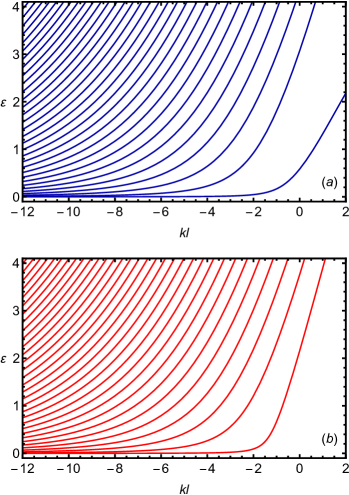
Figure 5: The energy spectra $\varepsilon(k)$ in the critical regime, $\beta=1$, near the zigzag edge of graphene’s half-plane for the gapless, $\Delta=0$ case. (a) For $\mathbf{K}_{+}$ valley, (b) For $\mathbf{K}_{-}$ valley.

The hole-like solutions that were present for $\beta<1$ and collapsing towards the $\varepsilon=0$ level in the $\beta\to 1$ limit are absent because there are no normalizable solutions of the original system in the $\beta=\pm 1$ cases. It is shown in Ref. [39] that the critical solutions, $\beta=\pm 1$, are not bound states.

One can easily see that Eqs. (48) and (50) for $kl=0$ reduce to Eqs. (67) and (71), respectively. Accordingly, the energies of the Landau levels at the edge in Fig. 4 (for $\beta=+1$) and Fig. 5 (for $kl=0$) are in agreement and tend to the values given by Eqs. (29) and (31). As discussed in the previous Section, these electron-like levels do not collapse at the edge, but now we may also follow their behavior in the bulk. One can see in Fig. 5 that these levels become denser and approach each other asymptotically as $kl\to-\infty$. This conclusion is confirmed by studying analytically Eqs. (48) and (50) in the limit $-kl=L/l$ for $L\gg l$ with $L$ being the distance from the edge. The derivation follows the approach to Eq. (31) and relies on the asymptotic expressions given by Eq. (68). It gives that the distance between the levels in the bulk is $\sim l^{3}/L^{3}$ for $L\gg l.$ This implies that there is no Landau level collapse of the electron-like states in the semi-infinite geometry for $\beta=1$. This conclusion is, however, correct in the formal mathematical sense, because the Landau levels of a finite width would anyway merge.

V.3 Specific of the Landau level collapse on the zigzag ribbon

The investigation of the energy levels on the ribbon was done either on the lattice fully numerically [13, 21, 22] or by solving transcendental equation as in Secs. S2 and S3. Although it allows to observe that the levels in certain regions of the ribbon become denser than in others, one cannot conclusively demonstrate that they collapse in a manner akin to what occurs in the case of an infinite system [see Eq. (1)]. In this respect, the analysis of the level behavior in the half-plane geometry in Secs. IV and VI is more convincing because it allows one to distinguish the level behavior in the $|\beta|\to 1$ limit.

Indeed, we have discovered that in the case of edges with bulk states situated on the left side, as the limit $\beta\to 1$ is approached, the hole-like levels collapse across the entire semi-plane. However, the point of the collapse, $\varepsilon=0$ and $\beta=1$, does not belong to the bound state spectrum. Conversely, the electron-like levels do not collapse at all. Their energies near the edge tend to the different values and deep within the bulk, when $-kl=L/l\gg 1$, the levels approach each other asymptotically with the distance between them $\sim l^{3}/L^{3}$.

Now we discuss the level behavior in the ribbon geometry. The critical regime, $\beta=1$, is shown in Fig. 6 for a ribbon of width $W=5l$ which is chosen to be smaller than for the rest of the figures for a better level resolution.

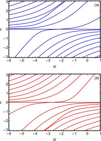
Figure 6: The energy spectra $\varepsilon(k)$ in the critical regime, $\beta=1$, of the zigzag ribbon of width $W=5l$ for the gapless, $\Delta=0$ case obtained by the numerical Eqs. (44) and (46). (a) For $\mathbf{K}_{+}$ valley, (b) For $\mathbf{K}_{-}$ valley.

First of all we observe that there is no Landau level collapse on the zigzag ribbons. While the hole-like levels were collapsing in the semi-infinite geometry, now they only become denser near the $kl=0$ edge.

This result can be qualitatively explained as follows: as observed earlier, in the semi-infinite geometry, the collapse of Landau levels happens when the center of the hole orbit remains in the bulk [$y>0$, see Eq. (19)]. For $\beta=1$ this is possible for hole-like states, but not for the electron-like ones. The presence of the other edge does not allow the hole orbit to remain inside the ribbon. We also note the interchange of electron- and hole-like levels at the opposite edge, as expected based on symmetry arguments.

To extend the analysis of Sec. V.2 of the level behavior in the bulk to the case of the ribbon, we consider Eqs. (44), (45), (46) and (47) from Sec. V. We obtain that for $\beta=1$ the distance between electron-like levels near $-kl=W/l$ edge is $O(l^{3}/W^{3})$ for $W>>l$. This confirms our statement that there is no Landau level collapse on the ribbons in a sense that all levels do not collapse to the lowest one. This conclusion is, however, correct only mathematically, because if the ribbon is wide enough the Landau levels of a finite width would anyway merge. On the other hand, we obtained that the correction to the non-collapsing solutions (29) is $O\left(e^{-4\sqrt{2|\varepsilon|}/3(W^{3}/l^{3})}\right)$.

VI Half-plane with the armchair edge

As was discussed in Sec. II.1, the armchair boundary conditions (8) admix the solutions for $\mathbf{K}_{\pm}$ valleys. Thus in addition to the solution (14) and (15) for $\mathbf{K}_{+}$ valley one needs the corresponding solutions (S7) and (S8) from [32] for $\mathbf{K}_{-}$ valley. The equation (S13) for the spectrum of the armchair ribbon undergoes significant simplification in the case of semi-infinite geometry, where $W\to\infty$. As discussed in Sec. IV for the half-plane with the zigzag edge, one may set $C_{+2}=C_{-2}=0$.

Now the boundary conditions (8) at $x=W\to\infty$ are automatically satisfied due to the asymptotic of $U(a,x\to\infty)$ and the remaining boundary conditions (8) at $x=0$ result in the following system of equations

$$C_{+1}\left[\gamma U\left(a-1,\sqrt{2}\zeta(0)\right)-\kappa_{+}U\left(a,\sqrt{2}\zeta(0)\right)\right]$$ (52)

$$+ C_{-1}\left[U\left((a-1,\sqrt{2}\zeta(0)\right)+\gamma\kappa_{-}U\left(a,\sqrt{2}\zeta(0)\right)\right]=0,$$

$$C_{+1}\left[U\left(a-1,\sqrt{2}\zeta(0)\right)-\gamma\kappa_{+}U\left(a,\sqrt{2}\zeta(0)\right)\right]$$

$$+ C_{-1}\left[\gamma U(a-1,\sqrt{2}\zeta(0))+\kappa_{-}U(a,\sqrt{2}\zeta(0))\right]=0.$$

The requirement for the system (52) to possess nontrivial solution results in the following equation for the spectrum:

$$U^{2}\left(a-1,\sqrt{2}\zeta(0)\right)+\left(a-\frac{1}{2}\right)U^{2}\left(a,\sqrt{2}\zeta(0)\right)=0.$$ (53)

It determines dimensionless energies $\varepsilon_{\alpha}=\varepsilon_{n}(kl)$ as functions of quantum numbers $\alpha\equiv n,k$ of a half-plane with the armchair edge.

The corresponding spectra are computed numerically and presented for the gapless and gapped cases in Figs. 7 and 8, respectively, where the dimensionless energy $\varepsilon(k)$ is plotted.

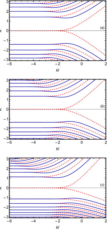
Figure 7: The energy spectra $\varepsilon(k)$ of the first few Landau levels near the armchair edge of graphene for the gapless, $\delta=0$ case. (a) $\beta=0$; (b) $\beta=0.25$; (c) $\beta=0.5$. The solid (blue) and the dashed (red) lines are solely used for a better resolution of the degenerate in the bulk solutions.

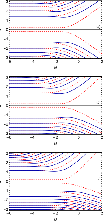
Figure 8: The energy spectra $\varepsilon(k)$ of the first few Landau levels near the armchair edge of graphene for the gapped, $\delta=0.2$ case. The panels (a), (b) and (c) are for the same values of $\beta$ as in Fig. 7.

Let us recapitulate the main specific features of these solutions. Since a half-plane geometry is considered, for a finite $\beta$ the energies $\varepsilon(k)$ tend to constant values in the bulk as $kl\to-\infty$. The levels which degeneracy was lifted by the edge become degenerate in the bulk. The armchair edge does not support the dispersionless mode. However, one of the solutions when approaching the edge shows a nonmonotonous behavior of the energy. This leads to a change in the sign of the drift velocity [26, 30].

VI.1 Zero electric field limit

In the absence of electric field, $\beta=0$, Eq. (53) preserves its form, but with $a=[1+\delta^{2}-\varepsilon^{2}]/2$ and $\zeta(0)=kl$ which agrees with the equation studied in Refs. [27, 28]. The corresponding numerical solutions shown in Figs. 2 (a) and 3 (a) are in agreement with the results presented in Refs. [24, 23, 27, 28].

VI.2 Finite electric field

As in Sec. IV.2, we show in Fig. 9 numerical solutions of Eq. (53) for the energy spectra at the armchair edge, $\varepsilon(kl=0)$, and $\delta=0$. These solutions are depicted as functions of $-1\leq\beta\leq 1$ for the first few Landau levels. We emphasize that for the armchair edge the solutions for $\mathbf{K}_{\pm}$ valleys are not separable and the panels (a) and (b) are solely used for a better readability.

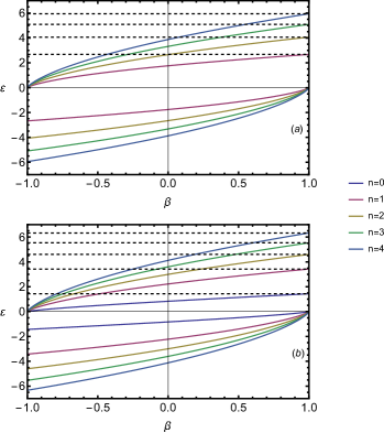
Figure 9: The energy spectra $\varepsilon(kl=0)$ at the armchair edge versus electric field in terms of $\beta=cE/(v_{F}H)$ for $\delta=0$ for first few Landau levels. (a) The dashed lines correspond to the energies given by the upper line of Eq. (54). (b) The dashed lines correspond to the energies given by the lower line of Eq. (54).

One can see that the behavior of the level energies at the edge is rather similar to the case of the zigzag edge. The electron-like levels collapse only for $\beta\to-1$, while for $\beta\to 1$ the levels do not collapse and their energies tend to the different values. On the contrary, the hole-like solutions merge and collapse for $\beta\to 1$, while for $\beta\to-1$ these levels do not collapse.

Similarly to the zigzag edge case, it is possible to consider analytically Eq. (53) at the edge, $kl=0$. The spectrum in the $\beta\to 1$ limit reads

$$\varepsilon_{n}=\begin{cases}\sqrt{2\varkappa^{3}_{1,n}},\\ \sqrt{2\varkappa^{3}_{2,n}},\end{cases}\qquad n=0,1,\ldots,$$ (54)

where $\varkappa_{1,n}$ and $\varkappa_{2,n}$ are the roots of the equations $\text{Ai}\left(-x^{2}\right)=0$ and $\text{Ai}^{\prime}\left(-x^{2}\right)=0$, respectively. These values of the energies corresponding to the upper and lower lines of Eq. (54) are shown in Figs. 9 (a) and (b), respectively, confirming a good agreement between the original equation for the spectrum and its $\beta\to 1$ limit. Finally, we obtain the following approximation for the solution (54)

$$\varepsilon_{n}^{\mathrm{app}}=\begin{cases}\sqrt{3\pi\left(n-\frac{1}{4}\right)},&n=1,2\ldots,\\ \sqrt{3\pi\left(n+\frac{1}{4}\right)},&n=0,1,\ldots\\ \end{cases}$$ (55)

which shows a good agreement with the results obtained solving numerically the full equation involving Airy function.

Although the complexity of the corresponding equations makes it impossible to analyze the level behavior for the armchair ribbon as was done for the zigzag ribbon, the presented results indicate that there is no Landau level collapse in armchair ribbons.

VII Summary

To conclude our main results can be summarized as follows:

1. The Landau level collapse in the restricted geometry occurs not in the same fashion as in the infinite geometry where it appears as a sharp transition.

2. In the semi-infinite geometry the hole (electron)-like Landau levels collapse as the ratio of electric and magnetic fields, $\beta=cE/v_{F}H$, reaches the critical value $+(-)1$. On the other hand, the energies of the electron (hole)-like levels near the edge remain different and are given by Eqs. (31) and (55) for the zigzag and armchair edges, respectively. The same levels deeply within the bulk, for $-kl=L/l\gg 1$, approach each other asymptotically.

3. There is no Landau level collapse on the ribbons, because in contrast to the semi-infinite geometry the orbit center cannot go to infinity. Instead, the electron (hole)-like levels become denser. The absence of collapse is, however, valid in a mathematical sense, because if the ribbon is wide enough the Landau levels of a finite width would anyway merge forming a band.

4. We derived the transcendental equations describing the Landau level behavior in the crossed magnetic and in-plane electric fields on the zigzag and armchair ribbons (see SM [32]) with the edges at $kl=0$ and $kl=-W/l$ and in the semi-infinite geometry, $W\to\infty$ [Eqs. (21), (22) and (53)]. These equations are analyzed analytically and numerically.

5. In particular, the simplified equations (44), (45), (46) and (47) in terms of the Airy functions describing the critical regime are obtained.

The obtained behavior of the Landau level collapse on the ribbons represents a particular example of describing systems of a finite size. As already mentioned in the Introduction, the Landau-level collapse was already observed experimentally [15, 16]. It would be useful to test the specific predictions made in the present work.

Appendix A Analytical study of the spectrum for semi-infinite system with zigzag edge, $kl=0$

For small values of $\beta$, Eqs. (21) and (22) can be solved by expanding the parabolic cylinder function $U(a,z)$ in the argument $z$ [see Eq. (19.3.5) in Ref.[37]]. In this case, we have

$$\sqrt{2}\zeta(0)\Big{|}_{kl=0}=\sqrt{2}\frac{\beta\varepsilon}{\left(1-\beta^{2}\right)^{3/4}}=\sqrt{2}\beta\varepsilon^{(0)}+o(\beta),\\$$ (56)

and

$$\begin{split}\kappa_{-}\kappa_{+}&=\frac{\delta^{2}\left(1-\beta^{2}\right)-\varepsilon^{2}}{2\left(1-\beta^{2}\right)^{3/2}}\\ &=\frac{1}{2}\left(\delta^{2}-(\varepsilon^{(0)})^{2}\right)-\varepsilon^{(0)}\varepsilon^{(1)}\beta+o(\beta),\end{split}$$ (57)

where $\varepsilon=\sum_{s=0}^{\infty}\varepsilon^{(s)}\beta^{s}$, $\varepsilon=\varepsilon(kl=0)$.

Then expanding the solutions for the $\mathbf{K}_{+}$-valley in the vicinity the $\beta=0$ solutions, $\varepsilon_{+,0}^{(0)}=-\delta$ and $(\varepsilon_{+,n}^{(0)})^{2}-\delta^{2}=4n$ with $n=1,2,\ldots$ (see Eq. (S17) in [32]) we obtain the following set of equations for $\varepsilon^{(1)}$:

$$\frac{\beta}{\Gamma\left(\frac{1}{2}\right)}=\varepsilon^{(1)}_{+,0}\beta,$$ (58)

$$\begin{split}\frac{\beta+2\beta\varepsilon^{(0)}_{+,n}\left(\delta+\varepsilon^{(0)}_{+,n}\right)}{\Gamma\left(\frac{1}{2}-n\right)}&=\\ \left(\delta+\varepsilon^{(0)}_{+,n}\right)(-1)^{n-1}&\Gamma(n)\left(-\frac{1}{2}\varepsilon^{(0)}_{+,n}\varepsilon^{(1)}_{+,n}\beta\right)\end{split}$$ (59)

Hence, we arrive at Eq. (27).

Similarly, for the $\mathbf{K}_{-}$-valley expanding in the vicinity of the solutions for $\beta=0$: $\varepsilon_{-,n}^{2}-\delta^{2}=2(2n+1)$ with $n=0,1,\ldots$ [see Eq. (S18) in [32]] we obtain the following set of equations for $\varepsilon^{(1)}$

$$\begin{split}&\frac{2\beta\varepsilon^{(0)}_{-,n}\left(\delta^{2}-(\varepsilon^{(0)}_{-,n})^{2}\right)-\beta\left(\delta-\varepsilon^{(0)}_{-,n}\right)}{4\Gamma\left(\frac{1}{2}-n\right)}\\ &=(-1)^{n}\Gamma(n+1)\left(-\frac{1}{2}\varepsilon^{(0)}_{-,n}\varepsilon^{(1)}_{-,n}\beta\right)\end{split}$$ (60)

and finally arrive at Eq. (28).

Let us consider electronic levels with $\varepsilon>0$ and $\delta=0$ in the limit $\beta\rightarrow 1$. We rewrite the arguments of the parabolic cylinder functions that enter Eqs. (21) and (22) as follows

$$\left.\begin{aligned} U\left(a,\sqrt{2}\zeta(0)\Big{|}_{kl=0}\right)&\\ U\left(a-1,\sqrt{2}\zeta(0)\Big{|}_{kl=0}\right)&\end{aligned}\right\}=U\left(-\frac{\lambda}{2}-\frac{\nu^{2}}{2},\sqrt{2}\beta\nu\right)=U\left(-\frac{\mu_{\lambda}^{2}}{2},\sqrt{2}\beta_{\lambda}\mu_{\lambda}\right),$$ (61)

where the following notations were introduced $\nu=\varepsilon\left(1-\beta^{2}\right)^{-3/4}$, $\mu_{\lambda}=\nu\sqrt{1+\frac{\lambda}{\nu^{2}}}$ and $\beta_{\lambda}=\beta\left(1+\frac{\lambda}{\nu^{2}}\right)^{-\frac{1}{2}}$ with $\lambda=\mp 1$.

According to Ref. [38], Eq. (12.10.35) [see also Eq. (3.1) in [40]] for $a=-\mu^{2}/2<0$, $-2\sqrt{-a}<\sqrt{2}\mu\beta<\infty$ and for large positive real values of $\mu$ one can use the asymptotic expansion of the parabolic cylinder function in terms of Airy functions $\text{Ai}(x)$ that for $\beta\in[-1+\epsilon,\infty[$ converges uniformly:

$$U\left(-\frac{1}{2}\mu^{2},\sqrt{2}\beta\mu\right)=2\pi^{\frac{1}{2}}\mu^{\frac{1}{3}}g(\mu)\phi(\zeta)\left[\text{Ai}\left(\mu^{\frac{4}{3}}\zeta\right)A_{\mu}(\zeta)+\frac{\text{Ai}^{\prime}\left(\mu^{\frac{4}{3}}\zeta\right)}{\mu^{\frac{8}{3}}}B_{\mu}(\zeta)\right],$$ (62)

where

$$\begin{split}&\zeta=-\left(\frac{3}{2}\eta\right)^{\frac{2}{3}},\qquad\eta=\frac{1}{2}\text{arccos}(\beta)-\frac{1}{2}\beta\sqrt{1-\beta^{2}},\qquad g(\mu)\sim 2^{-\frac{1}{4}\mu^{2}-\frac{1}{4}}e^{-\frac{1}{4}\mu^{2}}\mu^{\frac{1}{2}\mu^{2}-\frac{1}{2}}\left(\sum_{s=0}^{\infty}\frac{g_{s}}{\mu^{2s}}\right)^{-1},\\ &\phi(\zeta)=\left(\frac{-\zeta}{1-\beta^{2}}\right)^{\frac{1}{4}},\qquad A_{\mu}(\zeta)\sim\sum_{s=0}^{\infty}\frac{a_{s}(\zeta)}{\mu^{4s}},\qquad B_{\mu}(\zeta)\sim\sum_{s=0}^{\infty}\frac{b_{s}(\zeta)}{\mu^{4s}}\end{split}$$ (63)

and the coefficients $a_{s}(\zeta)$, $b_{s}(\zeta)$ and $g_{s}$ are given in Eqs. (3.9) and (2.8), respectively, from Ref. [40]. Taking the leading term of the expansion we obtain

$$\frac{U\left(-\frac{1}{2}\mu_{+}^{2},\sqrt{2}\beta_{+}\mu_{+}\right)}{U\left(-\frac{1}{2}\mu_{-}^{2},\sqrt{2}\beta_{-}\mu_{-}\right)}=\frac{g(\mu_{+})}{g(\mu_{-})}\frac{\mu^{\frac{1}{3}}_{+}\phi(\zeta_{+})\text{Ai}\left(\mu^{\frac{4}{3}}_{+}\zeta_{+}\right)}{\mu^{\frac{1}{3}}_{-}\phi(\zeta_{-})\text{Ai}\left(\mu^{\frac{4}{3}}_{-}\zeta_{-}\right)}\underset{\beta\rightarrow 1}{\sim}\frac{\nu}{\sqrt{2}}\frac{\text{Ai}\left(-\left(\frac{\varepsilon^{2}}{2}\right)^{\frac{2}{3}}\left(1+\frac{\sqrt{2}\sqrt{1-\beta}}{\varepsilon^{2}}\right)\right)}{\text{Ai}\left(-\left(\frac{\varepsilon^{2}}{2}\right)^{\frac{2}{3}}\left(1-\frac{\sqrt{2}\sqrt{1-\beta}}{\varepsilon^{2}}\right)\right)}.$$ (64)

Here $\zeta_{\pm}(\eta_{\pm})$ and $\eta_{\pm}$ are given by $\eta(\beta_{\pm})$ with $\eta(\beta)$ defined by Eq. (63) and we used the following limiting expressions necessary to calculate the ratio (64):

$$\begin{split}&\frac{\mu^{\frac{1}{3}}_{+}g(\mu_{+})}{\mu^{\frac{1}{3}}_{-}g(\mu_{-})}\underset{\nu\rightarrow+\infty}{\sim}\frac{\nu}{\sqrt{2}}\left(1-\frac{1}{6\nu^{2}}+O\left(\frac{1}{\nu^{4}}\right)\right),\qquad\eta\underset{\beta\rightarrow 1}{\sim}\frac{2\sqrt{2}}{3}(1-\beta)^{3/2}+O\left((1-\beta)^{5/2}\right),\\ &\frac{\phi(\zeta_{+})}{\phi(\zeta_{-})}\underset{\beta\rightarrow 1}{\sim}1-\frac{1}{10\nu^{2}}+O\left(\frac{1}{\nu^{4}}\right),\qquad\mu^{2}_{\lambda}\eta_{\lambda}\underset{\beta\rightarrow 1}{\sim}\nu^{2}\eta+\lambda\frac{\sqrt{1-\beta}}{\sqrt{2}}+O\left((1-\beta)^{3/2}\right),\\ &-\mu^{\frac{4}{3}}_{\lambda}\zeta_{\lambda}=\left(\frac{3}{2}\right)^{\frac{2}{3}}\left(\mu^{2}_{\lambda}\eta_{\lambda}\right)^{\frac{2}{3}}\underset{\beta\rightarrow 1}{\sim}\left(\frac{\varepsilon^{2}}{2}\right)^{\frac{2}{3}}\left(1+\lambda\frac{\sqrt{2}\sqrt{1-\beta}}{\varepsilon^{2}}+O\left((1-\beta)^{3/2}\right)\right).\end{split}$$ (65)

Since $\gamma\underset{\beta\rightarrow 1}{\sim}\left(1-\sqrt{2}\sqrt{1-\beta}+(1-\beta)+O\left((1-\beta)^{3/2}\right)\right)$, substituting the ratio (64) in Eq. (21) for the spectrum in $\mathbf{K}_{+}$ valley we obtain the equation

$$\frac{U\left(-\frac{1}{2}\mu_{+}^{2},\sqrt{2}\beta_{+}\mu_{+}\right)}{U\left(-\frac{1}{2}\mu_{-}^{2},\sqrt{2}\beta_{-}\mu_{-}\right)}-\frac{\nu}{\sqrt{2}\gamma}\underset{\beta\rightarrow 1}{\sim}-\frac{\nu}{\sqrt{2}}\left[\frac{\text{Ai}^{\prime}\left(-\left(\frac{\varepsilon^{2}}{2}\right)^{\frac{2}{3}}\right)}{\text{Ai}\left(-\left(\frac{\varepsilon^{2}}{2}\right)^{\frac{2}{3}}\right)}\left(\frac{\varepsilon^{2}}{2}\right)^{\frac{2}{3}}\frac{2}{\varepsilon^{2}}\sqrt{2}\sqrt{1-\beta}+\sqrt{2}\sqrt{1-\beta}\right]=0.$$ (66)

Hence, the spectrum for $\mathbf{K}_{+}$ valley is characterized by the zeros of the following equation:

$$\text{Ai}^{\prime}\left(-\left(\frac{\varepsilon^{2}}{2}\right)^{\frac{2}{3}}\right)+\left(\frac{\varepsilon^{2}}{2}\right)^{\frac{1}{3}}\text{Ai}\left(-\left(\frac{\varepsilon^{2}}{2}\right)^{\frac{2}{3}}\right)=0.$$ (67)

It is convenient to define in Eq. (30) the function $f_{+}$ and express the spectrum for the $\mathbf{K}_{+}$ valley via its zeros $\varkappa_{+,n}$. Then the full spectrum which includes also $\mathbf{K}_{-}$ valley [see Eq. (71) below] is represented by Eq. (29).

Furthermore, under the assumption that the energies $\varepsilon_{n}$ are large which is certainly valid for large $n$, Airy function and its derivative in Eq. (30) can be expanded as follows (see Eqs. (9.7.9) and (9.7.10) from [38]):

$$\text{Ai}\left(-x\right)\sim\frac{1}{\sqrt{\pi}x^{\frac{1}{4}}}\sin\left(\frac{2}{3}x^{3/2}+\frac{\pi}{4}\right),\quad\text{Ai}^{\prime}\left(-x\right)\sim-\frac{x^{\frac{1}{4}}}{\sqrt{\pi}}\cos\left(\frac{2}{3}x^{3/2}+\frac{\pi}{4}\right),\quad x\to\infty.$$ (68)

Then the equation $f_{+}(-(\varepsilon^{2}/2)^{2/3})=0$ for the spectrum reduces to the trigonometric one

$$-\cos\left(\frac{\varepsilon^{2}}{3}+\frac{\pi}{4}\right)+\sin\left(\frac{\varepsilon^{2}}{3}+\frac{\pi}{4}\right)=0$$ (69)

which has the following set of the solutions $\varepsilon_{+,n}^{\mathrm{app}}=\sqrt{3\pi n}$ with $n=0,1,\ldots$. This set of approximate solutions also contains the zero energy solution, $\varepsilon_{+,0}^{\mathrm{app}}=0$, while the full equation with the Airy function has the lowest energy solution $\varepsilon_{+,0}=0.58315$. Nevertheless, starting from $n=1$ the approximate solutions of the trigonometric equation (69) and the full equation with the Airy function demonstrate an excellent agreement: $\varepsilon_{+,1}^{\mathrm{app}}=3.06998$, $\varepsilon_{+,1}=3.06965$ and $\varepsilon_{+,2}^{\mathrm{app}}=4.34161$ and $\varepsilon_{+,2}=4.34119$. Thus it is enough to omit the $n=0$ solution of Eq. (69) for the $\mathbf{K}_{+}$ valley. Accordingly, we included in the upper line of Eq. (31) only the solutions with $n=1,2,\dots$.

Similarly, for the $\mathbf{K}_{-}$ valley we substitute the ratio (64) in Eq. (22) and obtain the following equation

$$\frac{U\left(-\frac{1}{2}\mu_{+}^{2},\sqrt{2}\beta_{+}\mu_{+}\right)}{U\left(-\frac{1}{2}\mu_{-}^{2},\sqrt{2}\beta_{-}\mu_{-}\right)}-\frac{\nu}{\sqrt{2}}\gamma\underset{\beta\rightarrow 1}{\sim}-\frac{\nu}{\sqrt{2}}\left[\frac{\text{Ai}^{\prime}\left(-\left(\frac{\varepsilon^{2}}{2}\right)^{\frac{2}{3}}\right)}{\text{Ai}\left(-\left(\frac{\varepsilon^{2}}{2}\right)^{\frac{2}{3}}\right)}\left(\frac{\varepsilon^{2}}{2}\right)^{\frac{2}{3}}\frac{2}{\varepsilon^{2}}\sqrt{2}\sqrt{1-\beta}-\sqrt{2}\sqrt{1-\beta}\right]=0.$$ (70)

the spectrum for $\mathbf{K}_{-}$ valley is characterized by the zeros of the following equation:

$$\text{Ai}^{\prime}\left(-\left(\frac{\varepsilon^{2}}{2}\right)^{\frac{2}{3}}\right)-\left(\frac{\varepsilon^{2}}{2}\right)^{\frac{1}{3}}\text{Ai}\left(-\left(\frac{\varepsilon^{2}}{2}\right)^{\frac{2}{3}}\right)=0$$ (71)

Accordingly, the spectrum for the $\mathbf{K}_{-}$ valley is expressed via the zeros $\varkappa_{-,n}$ of the function $f_{-}$ defined by Eq. (30).

Again using the large negative argument expansion (68) applicable for the large energies $\varepsilon_{n}$, one can simplify equation for the spectrum $f_{-}(-(\varepsilon^{2}/2)^{2/3})=0$ to the trigonometric one

$$-\cos\left(\frac{\varepsilon^{2}}{3}+\frac{\pi}{4}\right)-\sin\left(\frac{\varepsilon^{2}}{3}+\frac{\pi}{4}\right)=0.$$ (72)

Eq. (72) has the following set of the solutions $\varepsilon_{-,n}^{\mathrm{app}}=\sqrt{3\pi\left(n+1/2\right)}$ with $n=0,1,\ldots$ The comparison of the approximate solutions given by this set and the full equation with Airy function demonstrates a rather good agreement starting from the $n=0$ level: $\varepsilon_{-,0}^{\mathrm{app}}=2.1708$, $\varepsilon_{-,0}=2.15569$ and $\varepsilon_{-,1}^{\mathrm{app}}=3.75994$, $\varepsilon_{-,1}=3.75805$. Thus the whole set starting from $n=0$ can be used in the lower line of Eq. (31). One can check that there are no collapsing solutions $\varepsilon\sim(1-\beta^{2})^{3/4}$ in the $\beta\to 1$ case.

To analyze Eqs. (21) and (22) in the limit $\beta\rightarrow-1$ for the electronic levels it is necessary to choose the large positive $\mu$ expansion (3.16) of $U\left(-\frac{1}{2}\mu^{2},-\sqrt{2}\beta\mu\right)$ instead of employed above Eq. (62) which converges uniformly $\beta\in[-1+\epsilon,\infty[$. Then one can prove that the only electronic solutions in the limit $\beta\rightarrow-1$ are collapsing, viz. $\varepsilon\sim(1-\beta^{2})^{3/4}$.

Introducing $\nu$ defined below Eq. (61), one can rewrite Eqs. (21) and (22) for $\delta=0$ and $\beta=-1$ in the form $f(\nu)=0$, where the function

$$f(\nu)=\frac{U\left(-\frac{1}{2}-\frac{1}{2}\nu^{2},-\sqrt{2}\nu\right)}{U\left(\frac{1}{2}-\frac{1}{2}\nu^{2},-\sqrt{2}\nu\right)}+\frac{\nu}{\sqrt{2}}.$$ (73)

One can check that for $\nu>0$ this equation has an infinite set of zeros $\nu_{n}$:

$$\frac{\varepsilon}{(1-\beta^{2})^{3/4}}=\nu_{n}.$$ (74)

The values $\nu_{2n}$ with $n=1,2,\ldots$ correspond to the $\mathbf{K}_{+}$ valley and $\nu_{2n+1}$ with $n=0,1,\ldots$ correspond to the $\mathbf{K}_{-}$ valley, respectively. Thus we arrive at Eq. (32).

References

- [1] I. Rabi, Z. Phys. 49, 507 (1928).
- [2] V. Fock, Z. Phys. 47, 446 (1928).
- [3] Ya.I. Frenkel and M.P. Bronstein, J. Russian Phys. and Chem. Soc. (Physical section) 62, 485 (1930).
- [4] L.D. Landau, Z. Phys. 64, 629 (1930).
- [5] K.S. Novoselov, A.K. Geim, S.V. Morozov, D. Jiang, M.I. Katsnelson, I.V. Grigorieva, S.V. Dubonos, A.A. Firsov, Nature 438, 197 (2005).
- [6] Y. Zhang, Y.-W. Tan, H.L. Stormer, P. Kim, Nature 438, 201 (2005).
- [7] D.B. Chklovskii, B.I. Shklovskii, and L.I. Glazman, Phys. Rev. B 46, 4026 (1992).
- [8] G. Li, A. Luican-Mayer, D. Abanin, L. Levitov, E.Y. Andrei, Nat. Commun 4, 1744 (2013).
- [9] A. Coissard, A.G. Grushin, C. Repellin, L. Veyrat, K. Watanabe, T. Taniguchi, F. Gay, H. Courtois, H. Sellier, and B. Sacépé, Preprint arXiv:2210.08152
- [10] G. Nazin, Y. Zhang, L. Zhang, E. Sutter, and P. Sutter, Nature Physics 6, 870 (2010).
- [11] J.-P. Tetienne, N. Dontschuk, D. A. Broadway, A. Stacey, D. A. Simpson, and L. C. L. Hollenberg, Sci. Adv. 3, e1602429 (2017).
- [12] S. Kim, J. Schwenk, D. Walkup, et al., Nature Com. 12, 2852 (2021).
- [13] V. Lukose, R. Shankar, and G. Baskaran, Phys. Rev. Lett. 98, 116802 (2007).
- [14] N.M.R. Peres and E.V. Castro, J. Phys.: Condens. Matter 19, 406231 (2007).
- [15] V. Singh and M.M. Deshmukh Phys. Rev. B 80, 081404(R) (2009).
- [16] N. Gu, M. Rudner, A.Young, P. Kim, and L. Levitov Phys. Rev. Lett. 106, 066601 (2011).
- [17] Z.Z. Alisultanov, Physica B 438, 41 (2014).
- [18] A. Shytov, M. Rudner, N. Gu, M. Katsnelson, and L. Levitov, Sol. St. Commun. 149, 1087 (2009).
- [19] V. Arjona, E.V. Castro, and M.A.H. Vozmediano, Phys. Rev. B 96, 081110(R) (2017).
- [20] I.O. Nimyi, V. Könye, S.G. Sharapov, and V.P. Gusynin, Phys. Rev. B 106, 085401 (2022).
- [21] O. Roslyak, G. Gumbs, and D. Huang, Philos. Trans. R. Soc. London A 368, 5431 (2010).
- [22] B. Ostahie, M. Niţă, and A. Aldea, Phys. Rev. B 91, 155409 (2015).
- [23] L. Brey and H.A. Fertig, Phys. Rev. B 73, 195408 (2006).
- [24] D.A. Abanin, P.A. Lee, and L.S. Levitov, Phys. Rev. Lett. 96, 176803 (2006); Solid State Commun. 143, 77 (2007).
- [25] I. Romanovsky, C. Yannouleas, and U. Landman, Phys. Rev. B 83, 045421 (2011).
- [26] W. Wang and Z.S. Ma, Eur. Phys. J. B 81, 431 (2011).
- [27] V.P. Gusynin, V.A. Miransky, S.G. Sharapov, and I.A. Shovkovy, Phys. Rev. B 77, 205409 (2008).
- [28] V.P. Gusynin, V.A. Miransky, S.G. Sharapov, and I.A. Shovkovy, Fiz. Nizk. Temp. 34, 993 (2008). [English transl. Low Temp. Phys. 34, 778 (2008).]
- [29] V.P. Gusynin, V.A. Miransky, S.G. Sharapov, I.A. Shovkovy, and C.M. Wyenberg, Phys. Rev. B 79, 115431 (2009).
- [30] P. Delplace, G. Montambaux, Phys. Rev. B 82, 205412 (2010).
- [31] A.A. Herasymchuk, S.G. Sharapov, V.P. Gusynin, Physica Status Solidi (RRL) 2300084 (2023).
- [32] See Supplemental Material at http://link.aps.org/supplemental/ for additional details, which includes Refs. [37, 22, 13, 21, 23, 24, 35, 36, 31, 29, 30, 27, 28, 25].
- [33] V.P. Gusynin, S.G. Sharapov, and J. P. Carbotte, Int. J. Mod. Phys. B 21, 4611 (2007).
- [34] E. McCann and V.I. Fal’ko, J. Phys.: Condens. Matter 16, 2371 (2004).
- [35] L. Brey and H.A. Fertig, Phys. Rev. B 73, 235411 (2006).
- [36] M. Fujita, K. Wakabayashi, K. Nakada, and K. Kusakabe, J. Phys. Soc. Jpn. 65, 1920 (1996).
- [37] M. Abramowitz and I. A. Stegun, Handbook of Mathematical Functions With Formulas, Graphs, and Mathematical Tables (U.S. GPO, Washington, D.C., 1972), p. 685.
- [38] F.W. Olver, D.W. Lozier, R.F. Boisvert, and C.W. Clark, NIST Handbook of Mathematical Functions Hardback and CD-ROM by National Institute of Standards and Technology (U.S.) (Cambridge University Press, New York, 2010).
- [39] J.-Y. Cheng, Few-Body Syst 54, 1931 (2013).
- [40] N.M. Temme, J. Comput. Appl. Math. 121, 221 (2000).