Adaptive Splitting of Reusable Temporal Monitors for Rare Traffic Violations

Abstract

Autonomous Vehicles (avs) are often tested in simulation to estimate the probability they will violate safety specifications. Two common issues arise when using existing techniques to produce this estimation: If violations occur rarely, simple Monte-Carlo sampling techniques can fail to produce efficient estimates; if simulation horizons are too long, importance sampling techniques (which learn proposal distributions from past simulations) can fail to converge. This paper addresses both issues by interleaving rare-event sampling techniques with online specification monitoring algorithms. We use adaptive multi-level splitting to decompose simulations into partial trajectories, then calculate the distance of those partial trajectories to failure by leveraging robustness metrics from Signal Temporal Logic (stl). By caching those partial robustness metric values, we can efficiently re-use computations across multiple sampling stages. Our experiments on an interstate lane-change scenario show our method is viable for testing simulated av-pipelines, efficiently estimating failure probabilities for stl specifications based on real traffic rules. We produce better estimates than Monte-Carlo and importance sampling in fewer simulations.

I Statistical Simulation for AV Testing

Autonomous Vehicles (avs) typically undergo rigorous simulated testing before deployment [39]. A standard set of steps for testing is as follows: First we define a scenario (e.g., a highway lane-change expressed in OpenScenario [42]). Next, we define a safety specification (e.g., “avoid impeding traffic flow”) in a formal language like Signal Temporal Logic (stl). Then, we run stochastic simulations to estimate the probability our av-system violates our specification [11]. This statistical simulation approach is used because modern avs contain “black box” components like Neural-Network perception modules and non-linear solvers [45]. Such components provide few analytical guarantees over their behaviour.

A core problem plaguing statistical simulation is estimating rare events. Consider a stochastic simulation scenario where there exists a $10^{-4}$ probability that random noise in the sensors will cause our av to “fail” (i.e., to violate our safety specification). If we ran $100$ simulations, it is likely none would produce a failure. Even if sampling did produce a failure, estimation variance would be unacceptable [24].

Many works address rare-event problems for avs via Importance Sampling [25, 6]: Importance samplers draw simulations from a proposal distribution where the factors leading to a failure occur more frequently. The final estimate of failure probability is then re-weighted to reflect the original distribution. Since we do not know in advance all combinations of states which result in failure, such techniques must learn a good proposal. This learning step has no convergence guarantees, and probability estimates from such adaptive techniques can have unbounded error [3]. Importance sampling also tends to fare better when failures are caused by instantaneous single-state errors, but in the av domain, failures often occur as a result of accumulated errors over dependent states [9].

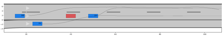
“Preserve Traffic Flow”

$$\centering\color[rgb]{.25,.25,.25}\scriptsize\square_{[0,\infty]}(\neg\text{slow\_leading\_vehicle}(x^{\textit{ego}},x^{o_{1}\dots o_{3}})\implies\text{preserves\_flow}(x^{\textit{ego}}))\@add@centering$$

Figure 1: Lane-change. Moving vehicles (blue) shown with trajectory. ‘Ego’ vehicle must avoid static obstacles (red). We monitor the safety constraint shown in English and stl.

This paper instead proposes an approach to av rare-event simulation based on merging Adaptive Multi-level Splitting (ams) [9] with stl monitoring. ams relies on estimating probabilities for a sequence of decreasing failure thresholds $\gamma_{1}>\gamma_{2}\dots>\gamma_{M}$, where the final $\gamma_{M}$ is equivalent to the rare failure event of interest. The key idea is that estimating any intermediate $\gamma_{i}$ (given $\gamma_{i-1}$) is easier than estimating $\gamma_{M}$ outright. To adapt ams from estimating isolated phenomena (e.g., particle transport [30]) to estimating complex av-system failures, we face two issues:

The main issue is how to consistently produce simulations which fall below those intermediate failure thresholds $\gamma_{0\dots M}$, and how to efficiently measure the distance to failure in the first place. Our approach measures failure using metrics for evaluating stl specification robustness. By leveraging online monitoring [13], we can cache the robustness values of partial trajectories, stop simulations at the point where they fall below the current threshold, and re-sample from this point onwards to produce trajectories which fall below subsequent failure thresholds.

A secondary issue is generating stochastic av perceptual errors. Approaches which assume noise follows a well-known (e.g., Gaussian) state-independent distribution [7] are insufficient to capture the perceptual variety of a typical av-system—a LiDAR detector may be great for close range traffic, but terrible for long range or occluded traffic [36]. We therefore use a Perception Error Model (pem) [37]—a surrogate trained on real sensor data which mimics perceptual errors encountered in regular operation (Sec II-A).

The main contribution of this paper is a new method for assessing failure probability in av-scenarios (Sec III), combining ams (Sec III-B), pems (Sec II-A), and online stl monitoring (Sec III-C). Our experiments focus on the case study of a highway lane-change scenario, and show our method can be used to test a full av-pipeline—perception down to control (Sec IV). Our approach outperforms Monte-Carlo sampling, as well as fixed and adaptive importance sampling, across various stl specifications (Sec IV-A).

To limit the scope of experiments, this paper exclusively considers probabilistic noise in the perception system as the primary source of simulation stochasticity (As is standard in other works [10]). However, our proposed sampling method can easily be applied to simulators which consider other sources of stochasticity such as those arising from traffic behaviour or physical uncertainties.

II Probability of Failure in Black Box Simulation

Consider the lane-change maneuver in Fig (1). Our car (the left-most ego vehicle), must change to the left lane to avoid an obstacle, then re-merge. Formally, let’s assume our scenario takes place over a total of $T$ time steps. We denote the $d$-dimensional state of our ego vehicle at time $t$ as $x^{ego}_{t}\in\mathds{R}^{d}$; other vehicles as $x^{o_{i}}_{t}$. For succinctness, we write $x_{t}=\{x^{ego}_{t},x^{o_{0}}_{t},\dots,x^{o_{M}}_{t}\}$ for the combined state. The state $x_{t}$ contains the position, velocity and rotation of each vehicle. At each time step $t$, the ego vehicle’s control system takes an action $a_{t}\in\mathds{R}^{2}$ (desired acceleration and turn-velocity) with the aim of minimizing costs associated with competing driving goals (e.g., maintaining a reference velocity and minimizing abrupt steering), and subject to constraints (e.g., limits on acceleration, avoiding collisions, staying within road boundaries). We can run a simulation of this system to generate a trajectory $\tau=[(x_{0},a_{0})\dots(x_{T},a_{T})]$, where $\tau_{[i{:}j]}=[(x_{i},a_{i})\dots,(x_{j},a_{j})]$) denotes a partial slice. For a given scenario, we wish to test whether our above av-system will violate an stl safety specification $\varphi$. Due to probabilistic noise in the perception system, our simulator is inherently stochastic. Therefore our aim is to calculate the probability that, for a random run of our simulator, our av-system will violate $\varphi$:

$$P_{\textit{fail}}=\mathds{E}\left[\mathds{1}\{\tau\nvDash\varphi\}\right]$$ (1)

Where $\mathds{1}\{\tau\nvDash\varphi\}$ is an indicator function which returns $1$ if $\tau$ violates $\varphi$ and $0$ otherwise. To explain how our method efficiently calculates (1), we first cover the pre-requisites for perception, tracking, and control for simulating our av (Sec II-A-II-B). We then cover defining safety specifications $\varphi$ in stl, and how to quantify their satisfaction using a robustness metric (III-A). We can then describe our main contribution—interleaving online monitoring and Adaptive Multi-level Splitting to estimate a failure probability for av-systems via statistical simulation (III-B).

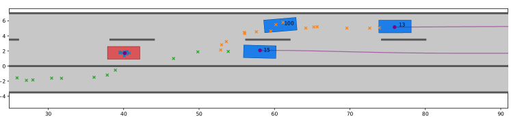
Figure 2: Lane change with pem observations, tracking, and prediction. Green/Orange crosses show pem obstacle observations. Purple dots/lines mark estimated/predicted positions.

II-A Simulated State Estimation with PEMs

Most av problems assume our system does not have access to the true state $x_{t}$. Instead our av must estimate this state via observations from its sensors (see Fig (2)). At time $t$, let us denote a full-snapshot of the world by $w_{t}$. This snapshot implicitly contains the relevant ground-truth state $x_{t}$, but also other scene information (e.g., vehicle types, dimensions etc.). A sensor $\mathcal{S}$ can be thought of as a function which takes $w_{t}$ and produces high-dimensional raw sensor data $\mathcal{S}(w_{t})$ (e.g., a LiDAR point-cloud). This sensor data is then passed to a perception function $f$ (e.g., a neural-network obstacle detector [38]), to produce an observation $y_{t}\in\mathbb{R}^{d^{\prime}}$ (e.g., the bounding boxes of other vehicles relative to the ego):

$$y_{t}=f(\mathcal{S}(w_{t}))$$ (2)

By using standard tracking algorithms [48], we can use these observations to get an estimate $\hat{x}_{t}$ of the current state:

$$\hat{x}_{t}=\mathds{E}\left[x\mid y_{0\dots t}\right]$$ (3)

If we have a one-step vehicle dynamics model $f_{\textit{dyn}}$, we can use it to predict the state in future time steps:

$$\hat{x}_{t+i\mid t}=\underbrace{f_{\textit{dyn}}\circ\dots\circ f_{\textit{dyn}}}_{\text{$i$ times}}(\hat{x}_{t})$$ (4)

Here, $\hat{x}_{t+i|t}$ denotes the predicted state at time $t$+$i$ given an estimate at $i$. In a real-world system, this setup allows us to sense, estimate, track and predict the state; in simulation, we have a problem: $f$ is typically a data-driven perception module trained on real sensors, but most simulators cannot generate high fidelity sensor inputs (e.g., photo-realistic images). We can resolve this issue by re-framing our perception system as a noisy projection from the state space to observation space:

$$y_{t}=f(\mathcal{S}(w_{t}))=Hx_{t}+\epsilon(g(w_{t})))$$ (5)

In this view, $f$ is composed of a $d^{\prime}\times d$ projection matrix $H$ on state $x_{t}$, plus stochastic error dependent on the current world state $w_{t}$. The $\epsilon$ function is a surrogate model known as a Perception Error Model [37]. This is a probabilistic model of the original av’s perception noise, dependent on salient features $g(w)$ extractable from simulated $w$. Salient features can include obstacle positions, dimensions, occlusion, or environment factors. We model $\epsilon$ as a gaussian process [49], where $m$, $\kappa$ are mean/kernel functions:

$$\epsilon(w)\sim\textsc{GP}(m(g(w)),\kappa(g(w),g(w^{\prime})))$$ (6)

Now, instead of using real-world sensor inputs directly, our simulator applies probabilistic noise from the pem based on the current simulated state. This makes each run of the simulator inherently stochastic, as different amounts of perceptual noise may be applied to observations on each run.

II-B Model Predictive Control for Highway Maneuvers

For a sufficiently complex control task such as lane changing, choosing the best actions $a_{t}$ at each time step is a non-linear constrained control task. We phrase the controller of our av system under test as a Receding-Horizon Model-Predictive Control optimization [41]. Eq (7) provides a formal definition of the optimization problem: At each time step $t$, the controller aims to choose actions $a_{t:(t+H)}$ over a finite time horizon $H$ which minimize a cost function $J(x,a)$. Actions must be chosen subject to a set of constraints $c_{j}(x,a)$ and obey physical dynamics $f_{dyn}$:

$$\begin{array}[]{@{}ll}\min\limits_{\begin{subarray}{c}x_{t:(t+H)}\\ a_{t:(t+H)}\end{subarray}}&\sum\limits_{k=t}^{t+H}J(x_{k},a_{k})\\ s.t.&x_{t}=\hat{x}_{t}\\ &\forall k,\ x_{k+1}=f_{\textit{dyn}}(x_{k},a_{k})\\ &\forall j,\ c_{j}(x_{k},a_{k})<0\\ \end{array}$$ (7)

Cost function $J(x,a)$ balances multiple factors such as tracking a reference velocity, minimizing abrupt movement, and staying close to the lane centre. The constraint functions $c_{j}(x,a)$ ensure states and actions remain feasible (e.g., that the car stays within road bounds and acceleration limits).

We give a further breakdown of the cost function and implementation in Section (IV). However, the purpose of describing Eq (7) here in the context of our testing problem is to highlight that our av-controller represents yet another “black-box” component of our system: Despite behaving deterministically, solvers for nonlinear control problems are not guaranteed to find a global solution, and can perform arbitrarily poorly [18]. Other typical methods (such as reinforcement learning), pose the same problem.

III Estimating Specification Failure Probability

We have defined our testing goal and outlined the components of our system-under-test. Now we can show how we formalize our safety properties, how we draw samples from the simulator, and how those aspects interact.

III-A Specifying Safety with Signal Temporal Logic

We can express av traffic rules involving statements about continuous values over time using Signal Temporal Logic [33]. stl has grammar:

$$\varphi:= \top\mid\eta\mid\neg\varphi\mid\varphi_{1}\wedge\varphi_{2}\mid\square_{I}\varphi\mid$$ (8)

$$\Diamond_{I}\varphi\mid\varphi_{1}\mathcal{U}_{I}\varphi_{2}\mid H_{I}\varphi\mid O_{I}\varphi$$

Here, $\eta$ is any predicate $\rho(s)-b\leq 0$ (with $b\in\mathbb{R}$ and $\rho:\mathcal{X}\rightarrow\mathbb{R}$). $\square_{I}\varphi$ means $\varphi$ is always true at every future time in interval $I$. $\Diamond_{I}\varphi$ means $\varphi$ must eventually be true in $I$, $\varphi_{1}\mathcal{U}_{I}\varphi_{2}$ means $\varphi_{1}$ must remain true within $I$ until $\varphi_{2}$ is true. $H_{I}$, $O_{I}$ are past versions of $\square_{I}$, $\Diamond_{I}$.

We can convert $\tau$ and $\varphi$ to a robustness metric $\mathcal{L}(\varphi,\tau,i)$ over trajectories [19]. This measures how strongly $\tau$ satisfied $\varphi$ (starting from time $i$). Large positive values indicate robust satisfaction; negative values a strong violation; near-zero values a trajectory on the boundary of satisfaction/violation. Eq (9) shows a subset of $\mathcal{L}$’s semantics. Other operators follow similar definitions [13].

$$\begin{array}[]{ll}\mathcal{L}(\rho(\tau)>0,\tau,i)&=\rho(x_{i})\\ \mathcal{L}(\neg\varphi,\tau,i)&=-\mathcal{L}(\varphi,\tau,i)\\ \mathcal{L}(\varphi_{1}\wedge\varphi_{2},\tau,i)&=\min(\mathcal{L}(\varphi_{1},\tau,i),\mathcal{L}(\varphi_{2},\tau,i))\\ \mathcal{L}(\square_{I}\varphi,\tau,i)&=\inf\limits_{i^{\prime}\in i+I}\mathcal{L}(\varphi,\tau,i^{\prime})\end{array}$$ (9)

III-B Estimating the Rare Event with Splitting

With our pem, av-controller, specification $\varphi$ and metric $\mathcal{L}$, we now describe our adaptive sampling contribution: Given $N$ simulated trajectories $\tau^{(1\dots N)}$, we wish to calculate Eq (1)—the probability a simulation violates $\varphi$. A naive approach might use Monte-Carlo sampling:

$$\mathds{E}\left[\mathds{1}\{\mathcal{L}(\varphi,\tau,0)<\gamma\}\right]\approx\frac{1}{N}\sum_{i=1}^{N}\mathds{1}\{\mathcal{L}(\varphi,\tau_{i},0)<\gamma\}$$ (10)

However, when violating $\varphi$ is rare, the number of simulations needed to achieve low relative error rapidly becomes infeasible [24]. We instead take a multi-level splitting approach [9]. Rather than immediately estimating failure ($\gamma=0$) we instead estimate decreasing thresholds $\gamma_{1}>\gamma_{2}>\dots>\gamma$. At each stage $m$, starting with $N$ trajectories we take two steps. First, we discard trajectories that do not fall below threshold $\gamma_{m}$. Second, we replenish back up to $N$ trajectories. To replenish discarded trajectories, we clone a random un-discarded $\tau^{(i)}$ up to $t^{\prime}$—the first time step where $\mathcal{L}(\tau^{(i)}_{[0{:}t^{\prime}]},\varphi,0)<\gamma_{m}$. Then, we re-simulate $\tau^{(i)}$ from $t^{\prime}$ to $T$. This ensures all $N$ trajectories at stage $m$ are below $\gamma_{m}$. With staged, partial re-samplings, Eq (1) becomes:

$$\prod\limits_{m=1}^{M}P(\mathcal{L}(\varphi,\tau,0)<\gamma_{m}|\mathcal{L}(\varphi,\tau,0)<\gamma_{m-1})$$ (11)

Given enough levels, each conditional probability should be significantly larger than $P(\mathcal{L}(\varphi,\tau,0)<\gamma)$. The final computation:

$$\hat{p}_{ams}=\left\{\prod^{M}_{m=1}\frac{N-K_{m}}{N}\right\}\times\frac{1}{N}\sum^{N}_{i=1}\mathds{1}\{\mathcal{L}(\varphi,\tau^{(i)},0)\}$$ (12)

has $M$ stages and $N$ initial simulations, where $K_{m}$ is the number discards per stage. Unlike adaptive importance sampling, ams guarantees convergence as $N\rightarrow\infty$ [8].

III-C Adaptive Splits via Online STL Monitors

To achieve our high-level goal of adapting ams to av testing of stl specifications, we currently face a slight computational dilemma: Our robustness metric $\mathcal{L}(\tau,\varphi,0)$ defines a single batch robustness value from the start to the end of a complete trajectory, and takes computation time proportional to the length of $\tau$. However in Section (III-B), we saw that the discard and replenishment steps require access to the robustness values at arbitrary prefixes of trajectories. In other words, ams re-simulation requires online computation of all partial trajectories:

$$\left\{\mathcal{L}(\tau^{(i)}_{[0{:}t^{\prime}]},\varphi,0)\mid t^{\prime}\in[0,T],i\in[0,N]\right\}$$ (13)

We resolve this dilemma by taking a key insight from the online monitoring literature—we can interleave partial computations into the ams process. To achieve this interleaving, we must first slightly alter our definition of $\mathcal{L}$ from (9) to define our metric in terms of partial rather than full trajectories. Eq (14) is a modified metric $\mathcal{L}_{n}$ (where $n$ references the “nominal semantics” of [13], augmented with past operators). This definition makes explicit that we only partially evaluate trajectory $\tau$ up to fixed time step $t$:

$$\begin{array}[]{@{}l@{}l@{}}\mathcal{L}_{\textit{n}}(\rho(x)>0,\tau_{[0{:}t]},i)&=\ \rho(\tau_{[i]})\\ \mathcal{L}_{\textit{n}}(\neg\varphi,\tau_{[0{:}t]},i)&=-\mathcal{L}_{\textit{n}}(\varphi,\tau_{[0{:}t]},i)\\ \mathcal{L}_{\textit{n}}(\square_{I}\varphi,\tau_{[0{:}t]},i)&=\inf\limits_{i^{\prime}\in(i+I\cap[0,t])}(\mathcal{L}_{\textit{n}}(\varphi,\tau_{[0{:}t]},i^{\prime}))\\ \mathcal{L}_{\textit{n}}(\Diamond_{I}\varphi,\tau_{[0{:}t]},i)&=\sup\limits_{i^{\prime}\in(i+I\cap[0,t])}(\mathcal{L}_{\textit{n}}(\varphi,\tau_{[0{:}t]},i^{\prime}))\\ \mathcal{L}_{\textit{n}}(O_{I}\varphi,\tau_{[0{:}t]},i)&=\sup\limits_{i^{\prime}\in(i-I\cap[0,t])}(\mathcal{L}_{\textit{n}}(\varphi,\tau_{[0{:}t]},i^{\prime}))\\ \mathcal{L}_{\textit{n}}(H_{I}\varphi,\tau_{[0{:}t]},i)&=\inf\limits_{i^{\prime}\in(i-I\cap[0,t])}(\mathcal{L}_{\textit{n}}(\varphi,\tau_{[0{:}t]},i^{\prime}))\\ \mathcal{L}_{\textit{n}}(\varphi_{1}\mathcal{U}_{I}\varphi_{2},\tau_{[0{:}t]},i)&=\sup\limits_{i_{2}\in(i+I\cap[0,t])}\min\left(\mathcal{L}_{\textit{n}}(\varphi_{2},\tau_{[0{:}t]},i_{2}),\vphantom{\inf\limits_{i_{i}\in[i,i_{2}]}}\right.\\ \end{array}$$ (14)

With the above definition, we could now naively compute all members of (13) by re-evaluating $\varphi$ at every $i$, up to every $t$, at every re-sampling step. This is computationally wasteful, as the robustness values of many partial trajectories share many operations with the computations of their prefixes. To take advantage of this fact, we instead maintain a work-list for each $\tau$. A work-list stores a mapping from specification $\varphi$ and time step $t$ to robustness value $\mathcal{L}_{n}(\varphi,\tau_{[0{:}t]},0)$. By using a work-list, we can obtain a robustness value for the partial trajectories at time $t$+$1$ using just the newly available state $x_{t+1}$ and the previous values of the work-list, rather than repeating computations over the entire trajectory.

Alg (1) takes as input the current work-list at time step $t$ and sketches how it is updated online using the newly arrived state $x_{t+1}$: For predicates $\rho(x)$, incoming state $x_{t+1}$ is added only if it is in $\varphi$’s time horizon. For example, for $\varphi=\square_{[0,2]}(\rho(x)>0)$, state $x_{3}$ would not be added, as it falls outside the relevant interval. For formulas like negation and conjunction, pointwise operators are leveraged to combine the existing results from previous sub-formula computations. Similarly for temporal operators, we can use the sliding min-max algorithm of [27] to compute running maxes over the relevant sub-formula intervals. Further optimizations can be added (e.g., replacing chunks of a work-list with ‘summaries’ as sufficient information arrives [13]) but we omit the details here. We can access the robustness of a partial trajectory from the updated work-list by querying $\textit{w-list}[\varphi][0]$.

1 Function upd-wl(w-list, $\varphi$, $x_{t+1}$)

2       switch $\varphi$ do

3             case $\rho(x)>0$ do

4                   if $t$+$1$ is within time horizon of $\varphi$ then  $\textit{w-list}[\varphi][t+1]\leftarrow\rho(x_{t+1})$ ;

5                  

6             case $\neg\psi$ do

7                   upd-wl(w-list, $\psi$, $x_{t+1}$)

8                  $\textit{w-list}[\varphi]\leftarrow$ Pointwise negation of $\textit{w-list}[\psi]$

9             case $\psi_{1}\wedge\psi_{2}$ do

10                   upd-wl(w-list, $\psi_{1}$, $x_{t+1}$)

11                  upd-wl(w-list, $\psi_{2}$, $x_{t+1}$)

12                  $\textit{w-list}[\varphi]\leftarrow$ Pointwise mins of $\textit{w-list}[\psi_{1}]$ and $\textit{w-list}[\psi_{2}]$

13             case $\square_{I}\psi$ do

14                   upd-wl(w-list, $\psi$, $x_{t+1}$)

15                  $\textit{w-list}[\varphi]\leftarrow\$Sliding min window of width $|I|$ across $\textit{w-list}[\psi]$

16             case $\Diamond_{I}\psi$ do

17                   upd-wl(w-list, $\psi$, $x_{t+1}$)

18                  $\textit{w-list}[\varphi]\leftarrow\$ Sliding max window of width $|I|$ across $\textit{w-list}[\psi]$

19            

20            case $\psi_{1}\mathcal{U}_{I}\psi_{2}$ do

21                   upd-wl(w-list, $\psi_{1}$, $x_{t+1}$)

22                  upd-wl(w-list, $\psi_{2}$, $x_{t+1}$)

23                  $\textit{lr-mins}\leftarrow$ Pointwise mins of $\textit{w-list}[\psi_{1}]$ and $\textit{w-list}[\psi_{2}]$

                  // Calculate backwards inductively

24                  

25                  for $i$ in descending timesteps do

26                         $\textit{us}[i]\leftarrow$$\max\left(\textit{lr-min}[i],\min(\textit{w-list}[\psi_{1}][i],us[i+1])\right)$

27                  $\textit{w-list}[\varphi]\leftarrow us$

28             case $H_{I}\psi$ do

29                   upd-wl(w-list, $\psi$, $x_{t+1}$)

30                  $\textit{w-list}[\varphi]\leftarrow$ Sliding min window of width $|I|$ across (reversed) $\textit{w-list}[\psi]$

31             case $O_{I}\psi$ do

32                   upd-wl(w-list, $\psi$, $x_{t+1}$)

33                  $\textit{w-list}[\varphi]\leftarrow$ Sliding max window of width $|I|$ across (reversed) $\textit{w-list}[\psi]$

34            

Algorithm 1 Update Work List (Adapted from [13])

1

2 Function stl-ams($x_{0}$, $\varphi$, $\gamma$, $T$, $K$, $N$)

3       for $i\in[1,N],t\in[0,T]$ do

4             $\epsilon_{t},y_{t},\hat{x}_{t},a_{t}\leftarrow$ Sample observations from PEM (5-6), track via (3) and choose actions by solving (7)

5            Append $\langle x_{t},a_{t}\rangle$ to trajectory $\tau^{(i)}$

            // Maintain work-list per trajectory (Alg 1)

6            

7            $\textit{w-list}^{(i)}_{t+1}\leftarrow$ upd-wl($\textit{w-list}^{(i)}_{t}$, $\varphi$, $x_{t+1}$)

            $L^{(i)}_{t+1}\leftarrow\textit{w-list}^{(i)}_{t+1}[\varphi][0]$ // Robustness of $\tau^{(i)}_{[0:t+1]}$

8            

9            $x_{t+1}\leftarrow$ Step forward simulation

10      Sort $\{L^{(0)}_{T}\dots L^{(N)}_{T}\}$ then set $\gamma_{0}\leftarrow L^{(K)}_{T}$

11      $m\leftarrow 0$

12      while $\gamma_{m}>\gamma$ do

13             $m\leftarrow m+1$

14            Discard all trajectories trajectories $\tau^{(i)}$ where $L^{(i)}_{T}\geq\gamma_{k}$

15            $\mathcal{I}_{k}\leftarrow$ Indices of remaining un-discarded trajectories

16            for $i\in[0,N]\setminus\mathcal{I}_{k}$ do

17                   Select a random $j\in{I}_{k}$

18                  Find the first time step $t^{\prime}$ where $L^{(j)}_{t^{\prime}}<\gamma_{k}$

19                  $\tau^{(i)}_{[0{:}t^{\prime}]},L^{(i)}_{[0{:}t^{\prime}]}\leftarrow$ Copy values from $\tau^{(j)}$

20                  $\tau^{(i)}_{[t^{\prime}{:}T]},L^{(i)}_{[t^{\prime}{:}T]}\leftarrow$ Re-simulate $\tau^{(j)}$ from time $t^{\prime}$

21            Sort $\{L^{(0)}_{T}\dots L^{(N)}_{T}\}$ then set $\gamma_{m}\leftarrow L^{(K)}_{T}$

22      return $\hat{p}_{ams}$ via Eqn (12)

Algorithm 2 Online stl-ams

Now that we can compute and cache stl robustness values for partial trajectories, we can interleave this with our ams sampler. Alg (2) provides an overview of our sampling technique for computing the probability that our av violates an stl specification in a stochastic simulation. It takes as input a starting state $x_{0}$, specification $\varphi$, failure threshold $\gamma$, initial simulation amount $N$ and discard rate $K$.

Lines (1-6) generate $N$ initial trajectories by simulating perceptual observations, control actions, and forward dynamics as outlined in sections (II-A-II-B). Lines (7-8) track the stl robustness value of trajectories at every intermediate time step by maintaining up-to-date work-lists as described in Alg (1). Lines (9, 17) adaptively set discard thresholds $\gamma_{m}$ such that the $K$ safest trajectories are discarded at each stage. To replenish those discarded trajectories, lines (14-16) copy one of the remaining un-discarded $\tau^{(i)}$ up until the first time step $j$ where the robustness value of the partial trajectory falls below $\gamma_{m}$. We then re-simulate starting from $j$ to produce a new trajectory. We repeat this process until the discard threshold $\gamma_{m}$ falls below the desired failure threshold $\gamma$, then calculate a final estimate $\hat{p}_{\textit{ams}}$ using Eq (12).

IV Experiments

The following experiments use our running example of an av lane-change maneuver to evaluate our method. They demonstrate that Alg (2) can provide failure estimates for a full black-box av-system across multiple common traffic rules. When compared to baselines, we find Alg (2) provides more accurate failure estimates in fewer simulations. Further, we investigate how sampling performance differs across discard-rates and rule types. Fig (1) shows our CommonRoad simulation setup [2]: The ego starts in the centre-lane at $15m$ with velocity $20\ m/s$. Its primary goal is to track a reference velocity of $v_{g}$=$30m/s$. Three obstacles impede it—a static obstacle at $40m$ (forcing the ego to change lanes); A centre-lane vehicle at $50m$ with velocity $5\ m/s$, which cuts into the overtake lane after $0.6$ seconds (slowing the ego or forcing a lane change); a right-lane vehicle at $50m$, velocity $10m$, which merges after $1$ second (preventing the ego from slowing abruptly). Simulations last $T$=$40$ steps ($4s$, $\Delta t$=$0.1s$). Dynamics evolve according to a kinematic single-track model [40].

Our av-system under test uses a standard pre-trained lidar-based obstacle detector—OpenPCDet’s Multi-Head PointPillar [26, 47]. As described in Section (II-A), we train a surrogate pem to replicate the behaviour of this detector in simulation. The pem is composed of two separate Gaussian Processes: The first is a binary classifier, which predicts whether the lidar perception system would have failed to detect a given obstacle. The second is a regression model, which predicts how much noise would typically be added to the true location of an obstacle’s bounding box. The gps were fitted using Pyro [4], with an rbf kernel and sparse variational regression with 100 inducing points. As training data for fitting the gps, we used $65500$ entries from the NuScenes Lidar Validation Set. The gp input features were a 7-d vector—the x/y obstacle position, rotation, length/width/height dimensions, obstacle “visibility category” (where “$1$” means $\leq 40\%$ occlusion; “$4$” means $\geq 80\%$). The gp outputs consist of a 1-d binary variable for successful/unsuccessful obstacle detection, and a 3-d real-valued variable for the offsets between the obstacle’s true x/y/rotation and the PointPillar estimate.

For tracking and predicting future vehicle locations, we used the interacting multiple models (imm) filter for lane-changes from [7]. This method operates similarly to a typical kalman filter, but instead of making estimates based on a single model, it maintains estimates from multiple models (i.e., for whether the vehicles will stay in the current lane, switch to the left lane, or switch to the right lane) and merges those estimates based on each model’s current likelihood.

For model predictive control (Eq (7)) we use the lane-change controller from [29]. At a high level, its cost function $J$ is comprised of 8 sub-goals: Reach a target destination; track a reference velocity, minimize acceleration, turn velocity, jerk and heading angle; stay close to the centre of the nearest lane; and avoid entering the “potential field” of other obstacles. To solve (7), we used the Gurobi [21] optimizer. To ensure a feasible control action is always available, we first pre-solve a convex simplification of (7) with CVXPy [14] (following [18]). For full implementation details of the cost-function sub-goals (and the weights used to balance them) see [29] and the associated code for our paper.

TABLE I: Interstate traffic rules (Predicate definitions in [32]).

Rule	Description	STL
$\varphi_{1}$	Safe Dist from Vehicles	$\begin{aligned} &\square_{[0,\infty]}(\texttt{in\_same\_lane}(x^{\textit{ego}},x^{o_{i}})\wedge\texttt{in\_front\_of}(x^{\textit{ego}},x^{o})\wedge\\ &\ \neg O_{[0,t_{\textit{cut}}]}(\texttt{cut\_in}(x^{o},x^{\textit{ego}})\wedge H_{[1,\infty]}(\neg\texttt{cut\_in}(x^{o},x^{\textit{ego}})))\\ &\ \implies\texttt{keeps\_safe\_distance\_prec}(x^{\textit{ego}},x^{o}))\end{aligned}$
$\varphi_{2}$	Unnecessary Braking	$\square_{[0,\infty]}\left(\neg\texttt{unnecessary\_braking}(x^{\textit{ego}},\{x^{o_{1},\dots,o_{3}}\})\right)$
$\varphi_{3}$	Preserve Traffic Flow	$\begin{aligned} &\square_{[0,\infty]}(\neg\texttt{slow\_leading\_vehicle}(x^{\textit{ego}},x^{o_{1}\dots o_{3}})\implies\texttt{preserves\_flow}(x^{\textit{ego}}))\end{aligned}$
$\varphi_{4}$	Don’t Drive Faster than Left Traffic	$\begin{aligned} &\square_{[0,\infty]}(\texttt{left\_of}(x^{o_{i}},x^{\textit{ego}})\wedge\texttt{drives\_faster}(x^{\textit{ego}},x^{o_{i}})\\ &\implies(\texttt{in\_slow\_traffic}(x^{o_{i}},x^{\{o_{1},\dots o_{3}\}\setminus x^{o_{i}}})\wedge\texttt{slightly\_higher\_speed}(x^{\textit{ego}},x^{o_{i}}))\\ &\quad\vee(\texttt{on\_access\_ramp}(x^{\textit{ego}})\wedge\texttt{on\_main\_carriageway}(x^{o_{i}})))\end{aligned}$

We test our sampling method with respect to 4 formalizations of rules from the Vienna Convention on Road Traffic (taken from [32]). Table (I) shows the stl for each rule. Full definitions of individual predicates (in_same_lane, drives_faster etc.) are in [32], but high level descriptions of each rule are as follows: $\bm{\varphi_{1}}$—maintain a minimum distance from vehicles in front (proportional to vehicle speed). If a vehicle “cuts in” from an adjacent lane, the ego gets $t_{\textit{cut}}$ seconds to re-establish distance. $\bm{\varphi_{2}}$—never drop acceleration below “unnecessary” levels (relative to vehicles in front). $\bm{\varphi_{3}}$—velocity should never fall below some minimum level (unless stuck in traffic). $\bm{\varphi_{4}}$—do not exceed the speed of left-lane vehicles unless merging from an access lane, or left-lane traffic is slow moving.

Our algorithm (listed as STL-AMS below) uses $N$=$250$ starting simulations, a discard amount of $K$=$25$, and final failure threshold of $\gamma=0$. We compare against three baselines: First, a Monte-Carlo sampler (Raw-MC), which runs $N$ simulations, estimating via (10). Second, an importance sampler with a fixed proposal (Imp-Naive). We choose a proposal distribution which deliberately fails to detect 50% of obstacles, and applies gaussian noise ($\mu$ = $0$, $\sigma^{2}$= $1$) to the bounding boxes of those it does detect. Third, a neural network-based importance sampler with an adaptive proposal learned via the cross-entropy method (Imp-CE) from [22]. Its inputs and outputs are the same as those of the gp-pem described previously. Similar to ams, adaptive importance sampling proceeds in stages: At each stage $m$ (for a total of $M=10$ stages), $N_{m}$=$250$ trajectories are sampled and sorted by robustness. Imp-CE then takes the lowest $K$=$0.1*N_{m}$ trajectories and minimizes their KL-divergence under the target pem versus current proposal. The intuition is that biasing our proposal towards the least robust trajectories in each stage should train a proposal which samples failure events with increasing probability.

IV-A Results and Discussion

TABLE II: Estimated Failure Probabilities (5 Repetitions)

Method	$\varphi_{1}$	$\varphi_{2}$	$\varphi_{3}$	$\varphi_{4}$
$\text{Raw-}\textsc{mc}_{250}$	$1.2\text{e-}02\ (\pm 4.0\text{e-}03)$	$0.0\ (\pm 0.0)$	$0.0\ (\pm 0.0)$	$0.0\ (\pm 0.0)$
Imp-Naive	$1.4\text{e-}08$ $(\pm 2.5\text{e-}08)$	$2.8\text{e-}08$ $(\pm 8.4\text{e-}08)$	$2.0\text{e-}08$ $(\pm 3.90\text{e-}08)$	$0.0$ $(\pm 0.0)$
Imp-ce	$7.1\text{e-}06$ $(\pm 2.1\text{e-}05)$	$7.6\text{e-}22$ $(\pm 2.2\text{e-}21)$	$4.4\text{e-}18$ $(\pm 8.9\text{e-}18)$	$0.0$ $(\pm 0.0)$
stl-ams (ours)	$8.8\text{e-}03$ $(\pm 6.2\text{e-}03)$	$1.5\text{e-}03$ $(\pm 2.1\text{e-}03)$	$4.7\text{e-}03$ $(\pm 3.4\text{e-}03)$	$3.5\text{e-}04$ $(\pm 1.8\text{e-}03)$
Ground Truth	$9.1\text{e-}03$	$2.0\text{e-}03$	$3.6\text{e-}03$	$4.8\text{e-}05$

Table (II) shows estimated probabilities per rule. For “ground-truth”, we computed Eq (10) using $100000$ simulations. Across rules, our method produces the most accurate estimates.

Raw-MC gives a reasonable estimate for $\varphi_{1}$ (the least rare). For other rules with lower probability, raw sampling yields zero simulation failures, resulting in $0\%$ estimates. Imp-Naive produces non-zero estimates for all specifications except $\varphi_{4}$, but vastly underestimates failure probability. This underscores the difficulty of fixed proposals—if a proposal distribution is too far from the original target, the likelihood weights per sample vary wildly, with estimates dominated by a tiny number of simulations. Imp-CE also produces unreliable estimates. Figs (3(a)-3(c)) provide insights why: As learning progresses for $\varphi_{3}$, the number of failures produced goes up, yet failure probability goes down. This suggests Imp-CE learns to bias its distribution towards a small set of unlikely failures, rather than approaching the true failure distribution. For $\varphi_{4}$, robustness thresholds initially decrease, but flatline around $m$=$6$—no failures found. We observe that this “flatlining” continues even past the $M=10$ stages documented in this paper. This highlights how challenging it can be to learn relevant features given longer horizons and state-spaces.

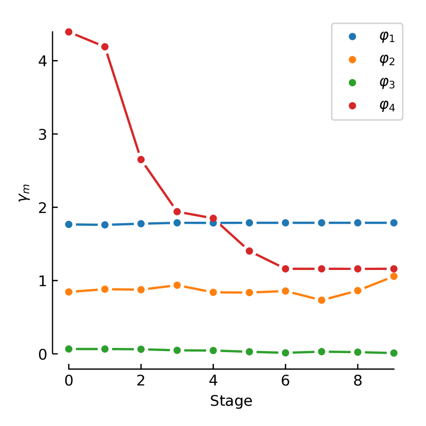
(a) Robustness Threshold

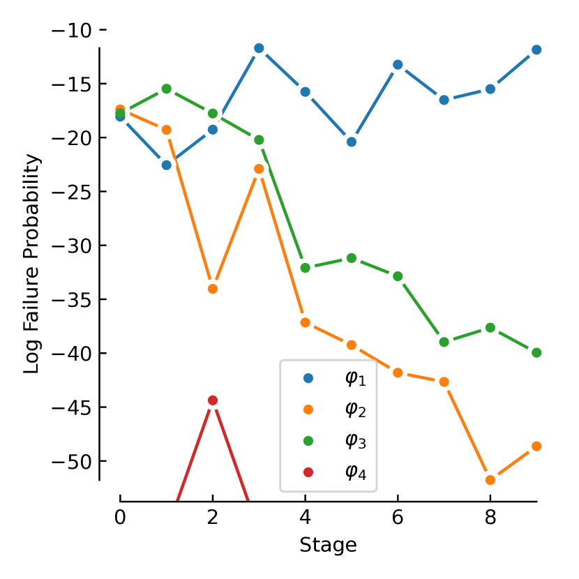
(b) Log Probs (-$\infty$ below axis)

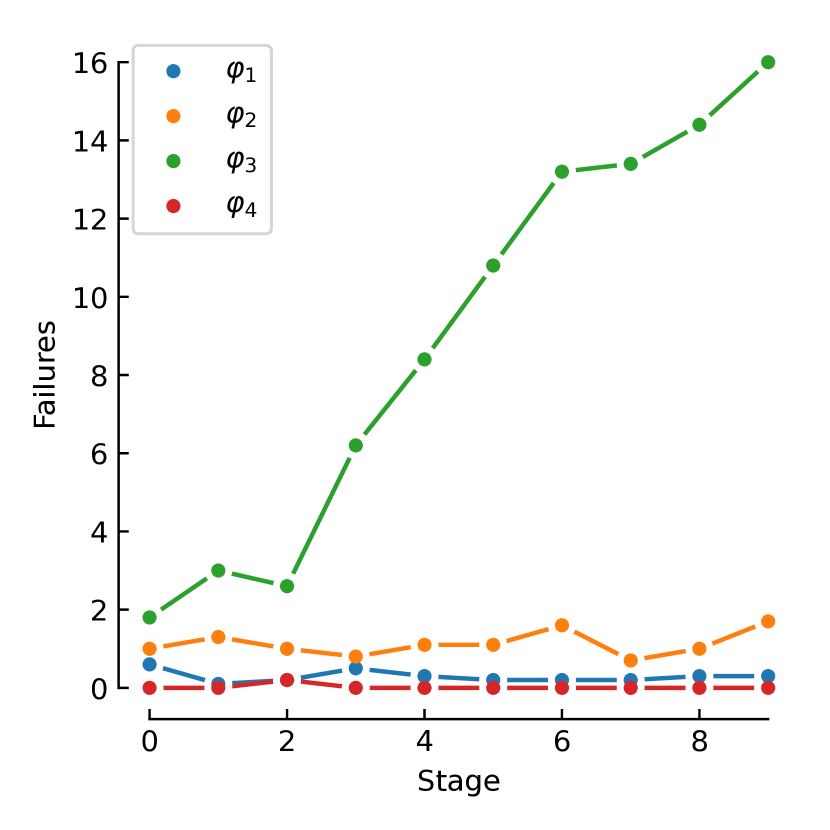
(c) Failures

Figure 3: Imp-CE baseline performance over 10 stages of proposal learning.

The results of Table (II) are encouraging, but we found Alg (2) was sensitive to discard rate $K$. Fig (4) shows how threshold levels evolve at each stage (for $K$ values from $2$ to $225$). For $\varphi_{4}$ (the rarest), we found that too low or high $K$s caused unacceptable numbers of “extinctions”[9]—stages where all trajectories have identical robustness, rendering replenishment impossible.

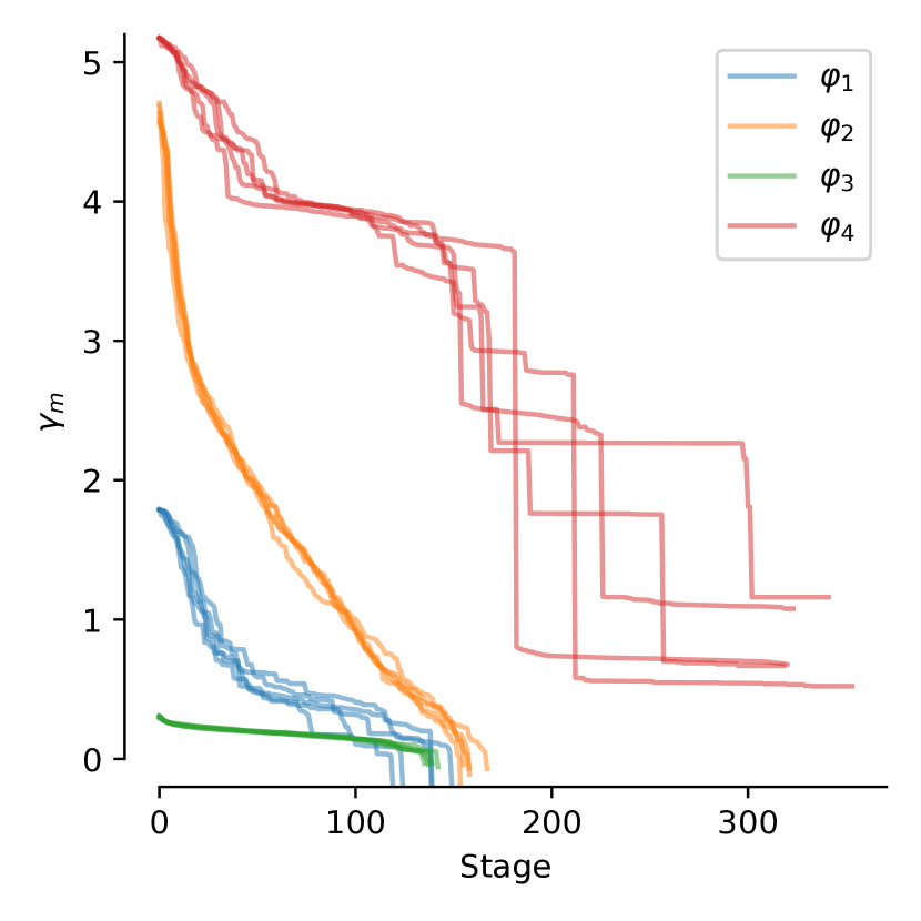
(a) $K=2$

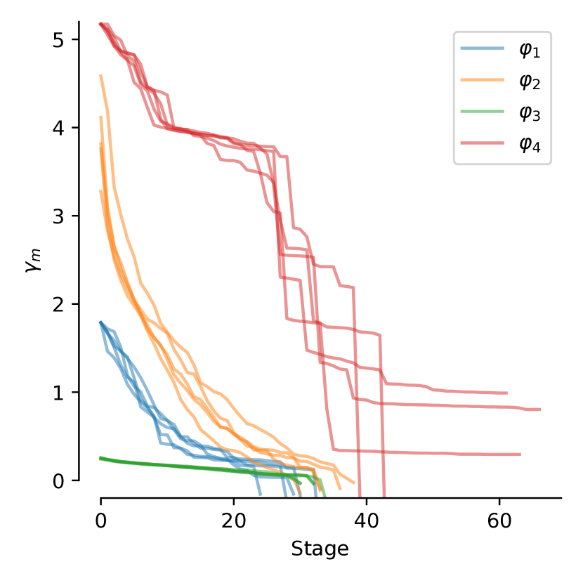
(b) $K=25$

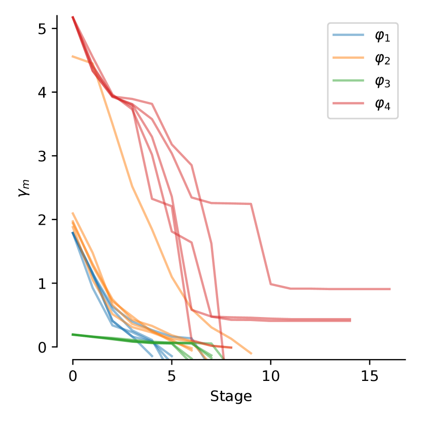
(c) $K=125$

(d) $K=225$

Figure 4: STL-AMS robustness thresholds by stage.

Experiments demonstrate Alg (2) is viable for accurately estimating specification failure for a black-box av-system. However, this case study looks only at a single interstate traffic scenario, and our experiments necessarily have limitations: We considered perceptual disturbance as the sole source of simulation stochasticity; vehicle starting configurations remained fixed. Such experiments could be extended by placing a prior distribution over starts [35], without altering the method. To trust our estimates, we also assume our simulator accurately represents reality. Whilst outside this paper’s scope, clearly this assumption may not hold: Our pem may be an inaccurate surrogate of the test domain (i.e., it would be beneficial to incorporate work on ml-uncertainty calibration [20]). Our scenario also had fixed traffic behaviour, but real traffic is reactive and stochastic. Other works explore these issues in detail [28]. Finally, while it can be seen as an advantage that our method adaptively selects an appropriate number of simulations, and re-uses results from previous simulations, these advantages complicate comparisons of our method to others in terms of sample efficiency. In future work, we aim to compare performance across a wider range of scenarios in terms of fixed computational effort across the full sampling pipeline.

V Related and Future Work

This paper estimates failure probabilities. Similar tasks include falsification (find one failure) and adaptive stress testing (find the most-likely failure) [11]. Such tasks do not directly accomplish our goal, but may contain insights for rapidly guiding initial simulations towards failure areas. A related task is synthesis—constructing controllers which explicitly obey $\varphi$ [1]. While synthesis can enforce adherence to specifications expressed in tractable stl subsets, the perceptual and control uncertainty in av scenarios means testing remains necessary.

Combining splitting and logic has been attempted previously [23]. Rather than use stl robustness, such works restrict themselves to heuristic decompositions of linear temporal logic formulae. This renders them unsuitable for cyber-physical domains like av.

One of our experiment baselines was importance sampling. Proposals are often represented by exponential distributions, since those have analytic solutions [44, 51]. Neural networks have also been used to represent the proposal (as we did), [34]. Most work considers rarity in the context of vehicle configurations or behaviour. Our work instead considers rarity in the context of perceptual disturbances. A sampler category unexplored in this paper are markov-chain methods [5]. With appropriate assumptions on metric smoothness and system linearizability, such techniques have shown promise in domains with long chains of dependent states [46, 43]. While out of scope, integrating such techniques with online stl monitoring may prove fruitful.

Despite the asymptotic normality of ams, both splitting and sampling lack guarantees on estimation error for fixed $N$. Certifiable sampling addresses this with efficiency certificates [3]—customized samplers with a bound on sampling error relative to $N$. However, certification methods depend on first being able to find the failure regions, so techniques from this paper remain relevant.

Online and offline algorithms exist to calculate stl robustness [16, 13]. Typically, efficiency is not considered in the context of a sampling regime. Yet recent advances in online monitoring could be leveraged within ams to discard infeasible trajectories early. For example, incorporating system dynamics, or causality [50, 12].

Our experiments target interstate lane changes. Others encode rules for intersections, and situational awareness [15, 31]. In future work, we aim to assess sampling effectiveness across this diversity of specifications.

References

- [1] Aasi, E., Vasile, C.I., Belta, C.: A control architecture for provably-correct autonomous driving. In: 2021 American Control Conference (ACC). pp. 2913–2918. IEEE (2021)
- [2] Althoff, M., Koschi, M., Manzinger, S.: Commonroad: Composable benchmarks for motion planning on roads. In: 2017 IEEE Intelligent Vehicles Symposium (IV). pp. 719–726. IEEE (2017)
- [3] Arief, M., Bai, Y., Ding, W., He, S., Huang, Z., Lam, H., Zhao, D.: Certifiable deep importance sampling for rare-event simulation of black-box systems. arXiv preprint arXiv:2111.02204 (2021)
- [4] Bingham, E., Chen, J.P., Jankowiak, M., Obermeyer, F., Pradhan, N., Karaletsos, T., Singh, R., Szerlip, P.A., Horsfall, P., Goodman, N.D.: Pyro: Deep universal probabilistic programming. J. Mach. Learn. Res. 20, 28:1–28:6 (2019), http://jmlr.org/papers/v20/18-403.html
- [5] Botev, Z.I., L’Ecuyer, P., Tuffin, B.: Markov chain importance sampling with applications to rare event probability estimation. Statistics and Computing 23, 271–285 (2013)
- [6] Bugallo, M.F., Elvira, V., Martino, L., Luengo, D., Miguez, J., Djuric, P.M.: Adaptive importance sampling: The past, the present, and the future. IEEE Signal Processing Magazine 34(4), 60–79 (2017)
- [7] Carvalho, A., Gao, Y., Lefevre, S., Borrelli, F.: Stochastic predictive control of autonomous vehicles in uncertain environments. In: 12th international symposium on advanced vehicle control. vol. 9 (2014)
- [8] Cérou, F., Guyader, A.: Fluctuation analysis of adaptive multilevel splitting. The Annals of Applied Probability 26(6), 3319 – 3380 (2016). https://doi.org/10.1214/16-AAP1177, https://doi.org/10.1214/16-AAP1177
- [9] Cérou, F., Guyader, A., Rousset, M.: Adaptive multilevel splitting: Historical perspective and recent results. Chaos: An Interdisciplinary Journal of Nonlinear Science 29(4) (2019)
- [10] Corso, A., Lee, R., Kochenderfer, M.J.: Scalable autonomous vehicle safety validation through dynamic programming and scene decomposition. In: 2020 IEEE 23rd International Conference on Intelligent Transportation Systems (ITSC). pp. 1–6. IEEE (2020)
- [11] Corso, A., Moss, R., Koren, M., Lee, R., Kochenderfer, M.: A survey of algorithms for black-box safety validation of cyber-physical systems. Journal of Artificial Intelligence Research 72, 377–428 (2021)
- [12] Deng, Z., Eshima, S.P., Nabity, J., Kong, Z.: Causal signal temporal logic for the environmental control and life support system’s fault analysis and explanation. IEEE Access 11, 26471–26482 (2023)
- [13] Deshmukh, J.V., Donzé, A., Ghosh, S., Jin, X., Juniwal, G., Seshia, S.A.: Robust online monitoring of signal temporal logic. Formal Methods in System Design 51, 5–30 (2017)
- [14] Diamond, S., Boyd, S.: CVXPY: A Python-embedded modeling language for convex optimization. Journal of Machine Learning Research 17(83), 1–5 (2016)
- [15] Dokhanchi, A., Amor, H.B., Deshmukh, J.V., Fainekos, G.: Evaluating perception systems for autonomous vehicles using quality temporal logic. In: Runtime Verification: 18th International Conference, RV 2018, Limassol, Cyprus, November 10–13, 2018, Proceedings 18. pp. 409–416. Springer (2018)
- [16] Donzé, A., Ferrere, T., Maler, O.: Efficient robust monitoring for stl. In: Computer Aided Verification: 25th International Conference, CAV 2013, Saint Petersburg, Russia, July 13-19, 2013. Proceedings 25. pp. 264–279. Springer (2013)
- [17] Duvenaud, D.: Automatic model construction with Gaussian processes. Ph.D. thesis, University of Cambridge (2014)
- [18] Eiras, F., Hawasly, M., Albrecht, S.V., Ramamoorthy, S.: A two-stage optimization-based motion planner for safe urban driving. IEEE Transactions on Robotics 38(2), 822–834 (2021)
- [19] Fainekos, G.E., Pappas, G.J.: Robustness of temporal logic specifications for continuous-time signals. Theoretical Computer Science 410(42), 4262–4291 (2009)
- [20] Guo, C., Pleiss, G., Sun, Y., Weinberger, K.Q.: On calibration of modern neural networks. In: International conference on machine learning. pp. 1321–1330. PMLR (2017)
- [21] Gurobi Optimization, LLC: Gurobi Optimizer Reference Manual (2023), https://www.gurobi.com
- [22] Innes, C., Ramamoorthy, S.: Testing rare downstream safety violations via upstream adaptive sampling of perception error models. In: 2023 IEEE International Conference on Robotics and Automation (ICRA). pp. 12744–12750. IEEE (2023)
- [23] Jegourel, C., Legay, A., Sedwards, S.: An effective heuristic for adaptive importance splitting in statistical model checking. In: International Symposium On Leveraging Applications of Formal Methods, Verification and Validation. pp. 143–159. Springer (2014)
- [24] Juneja, S., Shahabuddin, P.: Rare-event simulation techniques: An introduction and recent advances. Handbooks in operations research and management science 13, 291–350 (2006)
- [25] Kim, Y., Kochenderfer, M.J.: Improving aircraft collision risk estimation using the cross-entropy method. Journal of Air Transportation 24(2), 55–62 (2016)
- [26] Lang, A.H., Vora, S., Caesar, H., Zhou, L., Yang, J., Beijbom, O.: Pointpillars: Fast encoders for object detection from point clouds. In: Proceedings of the IEEE/CVF conference on computer vision and pattern recognition. pp. 12697–12705 (2019)
- [27] Lemire, D.: Streaming maximum-minimum filter using no more than three comparisons per element. arXiv preprint cs/0610046 (2006)
- [28] Li, J., Sun, L., Zhan, W., Tomizuka, M.: Interaction-aware behavior planning for autonomous vehicles validated with real traffic data. In: Dynamic Systems and Control Conference. vol. 84287, p. V002T31A005. American Society of Mechanical Engineers (2020)
- [29] Liu, C., Lee, S., Varnhagen, S., Tseng, H.E.: Path planning for autonomous vehicles using model predictive control. In: 2017 IEEE Intelligent Vehicles Symposium (IV). pp. 174–179. IEEE (2017)
- [30] Louvin, H., Dumonteil, E., Lelièvre, T., Rousset, M., Diop, C.M.: Adaptive multilevel splitting for monte carlo particle transport. In: EPJ Web of Conferences. vol. 153, p. 06006. EDP Sciences (2017)
- [31] Maierhofer, S., Moosbrugger, P., Althoff, M.: Formalization of intersection traffic rules in temporal logic. In: 2022 IEEE Intelligent Vehicles Symposium (IV). pp. 1135–1144. IEEE (2022)
- [32] Maierhofer, S., Rettinger, A.K., Mayer, E.C., Althoff, M.: Formalization of interstate traffic rules in temporal logic. In: 2020 IEEE Intelligent Vehicles Symposium (IV). pp. 752–759. IEEE (2020)
- [33] Maler, O., Nickovic, D.: Monitoring temporal properties of continuous signals. In: International Symposium on Formal Techniques in Real-Time and Fault-Tolerant Systems. pp. 152–166. Springer (2004)
- [34] Müller, T., McWilliams, B., Rousselle, F., Gross, M., Novák, J.: Neural importance sampling. ACM Transactions on Graphics (ToG) 38(5), 1–19 (2019)
- [35] O’Kelly, M., Sinha, A., Namkoong, H., Tedrake, R., Duchi, J.C.: Scalable end-to-end autonomous vehicle testing via rare-event simulation. Advances in neural information processing systems 31 (2018)
- [36] Pandharipande, A., Cheng, C.H., Dauwels, J., Gurbuz, S.Z., Ibanez-Guzman, J., Li, G., Piazzoni, A., Wang, P., Santra, A.: Sensing and machine learning for automotive perception: A review. IEEE Sensors Journal 23(11), 11097–11115 (2023). https://doi.org/10.1109/JSEN.2023.3262134
- [37] Piazzoni, A., Cherian, J., Dauwels, J., Chau, L.P.: Pem: Perception error model for virtual testing of autonomous vehicles. IEEE Transactions on Intelligent Transportation Systems (2023)
- [38] Qi, C.R., Yi, L., Su, H., Guibas, L.J.: Pointnet++: Deep hierarchical feature learning on point sets in a metric space. Advances in neural information processing systems 30 (2017)
- [39] Rajabli, N., Flammini, F., Nardone, R., Vittorini, V.: Software verification and validation of safe autonomous cars: A systematic literature review. IEEE Access 9, 4797–4819 (2020)
- [40] Rajamani, R.: Vehicle dynamics and control. Springer Science & Business Media (2011)
- [41] Rawlings, J.B., Mayne, D.Q., Diehl, M.: Model predictive control: theory, computation, and design, vol. 2. Nob Hill Publishing Madison, WI (2017)
- [42] Riedmaier, S., Ponn, T., Ludwig, D., Schick, B., Diermeyer, F.: Survey on scenario-based safety assessment of automated vehicles. IEEE access 8, 87456–87477 (2020)
- [43] Scher, G., Sadraddini, S., Tedrake, R., Kress-Gazit, H.: Elliptical slice sampling for probabilistic verification of stochastic systems with signal temporal logic specifications. In: Proceedings of the 25th ACM International Conference on Hybrid Systems: Computation and Control. pp. 1–11 (2022)
- [44] Schmerling, E., Pavone, M.: Evaluating trajectory collision probability through adaptive importance sampling for safe motion planning. arXiv preprint arXiv:1609.05399 (2016)
- [45] Schwarting, W., Alonso-Mora, J., Rus, D.: Planning and decision-making for autonomous vehicles. Annual Review of Control, Robotics, and Autonomous Systems 1, 187–210 (2018)
- [46] Sinha, A., O’Kelly, M., Tedrake, R., Duchi, J.C.: Neural bridge sampling for evaluating safety-critical autonomous systems. Advances in Neural Information Processing Systems 33, 6402–6416 (2020)
- [47] Team, O.D.: Openpcdet: An open-source toolbox for 3d object detection from point clouds. https://github.com/open-mmlab/OpenPCDet (2020)
- [48] Thrun, S.: Probabilistic robotics. Communications of the ACM 45(3), 52–57 (2002)
- [49] Williams, C.K., Rasmussen, C.E.: Gaussian processes for machine learning, vol. 2. MIT press Cambridge, MA (2006)
- [50] Yu, X., Dong, W., Yin, X., Li, S.: Online monitoring of dynamic systems for signal temporal logic specifications with model information. In: 2022 IEEE 61st Conference on Decision and Control (CDC). pp. 1553–1559. IEEE (2022)
- [51] Zhao, D., Lam, H., Peng, H., Bao, S., LeBlanc, D.J., Nobukawa, K., Pan, C.S.: Accelerated evaluation of automated vehicles safety in lane-change scenarios based on importance sampling techniques. IEEE transactions on intelligent transportation systems 18(3), 595–607 (2016)