\fnm

Rachel \surCarrington*

Post-selection inference for quantifying uncertainty in changes in variance

r.j.carrington@lancaster.ac.uk โ€ƒโ€ƒ \fnmPaul \surFearnhead p.fearnhead@lancaster.ac.uk \orgdivDepartment of Mathematics and Statistics, \orgnameLancaster University, \countryUK
Abstract

Quantifying uncertainty in detected changepoints is an important problem. However it is challenging as the naive approach would use the data twice, first to detect the changes, and then to test them. This will bias the test, and can lead to anti-conservative p๐‘p-values. One approach to avoid this is to use ideas from post-selection inference, which conditions on the information in the data used to choose which changes to test. As a result this produces valid p๐‘p-values; that is, p๐‘p-values that have a uniform distribution if there is no change. Currently such methods have been developed for detecting changes in mean only. This paper presents two approaches for constructing post-selection p๐‘p-values for detecting changes in variance. These vary depending on the method use to detect the changes, but are general in terms of being applicable for a range of change-detection methods and a range of hypotheses that we may wish to test.

keywords:
Changepoint detection; Breakpoint; Binary segmentation; Post-selection p๐‘p-value

1 Introduction

The problem of detecting changes in time series has received a great deal of attention in recent years, with applications in finance [33], quality control [2], climate modelling [31, 32], genome sequencing [26, 5], neuroscience [1], and epidemic modelling [21], amongst many others. Various methods have been developed for detecting different types of change, for example changes in mean, variance, and slope. These are often developed based on developing a test for a single change of a specific type. To detect multiple changes, this test can be used recursively within algorithms such as binary segmentation [35] and its variants such as wild binary segmentation [14], seeded binary segmentation [22], and narrowest over threshold [3]. Alternatively one can write down a likelihood for the data as a function of the number and location of changes and aim to estimate the changes by minimising a penalised version of this likelihood โ€“ for many models this optimisation can be performed exactly, see [23, 28]. See [13] and [34] for recent reviews of changepoint methods.

Recently, increasing attention has been given to the problem of estimating the uncertainty associated with detected changepoints [12, 25, 7]. This is challenging due to the interplay of different elements of uncertainty, in terms of the number and location of the changepoints. Bayesian approaches [4, 11, 30, 8] give a natural way of quantifying this uncertainty, but require specifying prior information with the results sensitive to these choices. Alternatively one can use the properties of test statistics under the assumption of no changepoints. For example, [15] and [16] use a probabilistic bound on the maximum of the test statistic for the presence of a change over all possible intervals of data to find the narrowest set of intervals which each must contain at least one changepoint with a certain probability. Similar bounds are used within the MOSUM method [29] to produce asymptotic p๐‘p-values for detected changepoints [10].

In this paper we consider a related approach, of post-selection inference [24]. The idea is to construct a p๐‘p-value for each detected changepoint, with the these p๐‘p-values being valid in finite samples, albeit under strong distributional assumptions for the data. This is a challenging problem in general as, if we were to use the data to estimate changepoint locations, naively re-using the same data to estimate the uncertainty associated with each changepoint will lead to biased results. The idea of post-selection inference is, when testing for the presence of a changepoint at some detected location ฯ„๐œ\tau, we condition on the information in the data that led to detection at ฯ„๐œ\tau when calculating the p๐‘p-value. To date, almost all work in this area has focused on the univariate change in mean case, e.g. [18, 20, 9, 6], or the piecewise constant polynomial model [27]. As far as we know, there are no current approaches for quantifying the evidence for detected changes in variance. In this paper we fill this gap by extending the post-selection inference ideas to cover the change in variance setting.

The post-selection inference methods for the change in mean problem use the fact that the natural test statistic for a change at a given location will have a standard normal distribution under the null. To account for the fact that we have used the same data to detect changes and thus to decide which locations to test, we need to condition this distribution on the fact that the tested location is a detected changepoint. This leads to a conditional null distribution that is constrained to lie on an interval [18] or a union of intervals [20] of the real line โ€“ depending on precisely what information is conditioned on. Importantly it is straightforward to calculate this interval or intervals for methods for detecting a change in mean that use the popular CUSUM statistic within a binary segmentation algorithm or within a penalised likelihood approach. One of the advantages of this approach is that it is general: it applies to a wide range of methods for detecting changes, and also to most natural null hypotheses that one may wish to test.

In this paper, we consider the two most common ways of detecting a change in variance. The first uses the idea that a change in variance in some time series, Xtsubscript๐‘‹๐‘กX_{t} say, will correspond to a change in mean in Xt2superscriptsubscript๐‘‹๐‘ก2X_{t}^{2}. Thus we can shift the data so it has mean zero, and apply a method for detecting a change in mean to the square of this shifted data. The second method is where we estimate changepoint locations by directly maximizing the likelihood of the piecewise constant variance model. In both cases we then use the same test statistic for testing whether a detected change is real. This test statistic is equivalent to the likelihood-ratio test statistic for a change in variance in Gaussian data, and is the proportion of the sum of squares of the data in the region prior to the putative change. If we had used separate information, or independent data, to choose which putative change location to test then the null distribution of this test statistic a Beta distribution with known parameters. For our setting we need to calculate the null distribution conditional on detecting the change, which leads to constraining the Beta distribution to a union of intervals of [0,1]01[0,1].

To calculate the post-selection p๐‘p-values requires us to calculate these intervals. For the first approach to detecting changes, this can be done analytically using the same ideas as for the change in mean setting. For the second approach, this is no longer possible so we show how Monte Carlo can be used to approximate the p๐‘p-values [see 36, for similar use of Monte Carlo in post-selection inference].

The rest of the paper is organized as follows. In Section 2 we define the model and set up the test we will use to detect changes in variance. Section 3 then describes the methods we will use to calculate p๐‘p-values. Section 4 details some extensions to different scenarios, such as different null hypotheses and changepoint detection methods. Section 5 presents results of our methods on simulated data, and in Section 6 we implement our method on a financial data set. Section 7 then concludes with some discussion of our results and suggestions for further research.

2 Testing for a change in variance

We consider the univariate Gaussian model with fixed mean and piecewise constant variance:

Xt=ฮผ+ฯƒtโ€‹ฯตt,t=1,โ€ฆ,T,formulae-sequencesubscript๐‘‹๐‘ก๐œ‡subscript๐œŽ๐‘กsubscriptitalic-ฯต๐‘ก๐‘ก1โ€ฆ๐‘‡X_{t}=\mu+\sigma_{t}\epsilon_{t},~{}~{}t=1,\ldots,T, (1)

where ฮผ๐œ‡\mu is assumed known, ฯตtโˆผNโ€‹(0,1)similar-tosubscriptitalic-ฯต๐‘ก๐‘01\epsilon_{t}\sim N(0,1), and ฯƒt+1=ฯƒtsubscript๐œŽ๐‘ก1subscript๐œŽ๐‘ก\sigma_{t+1}=\sigma_{t} except at K๐พK changepoints {ฯ„1,โ€ฆ,ฯ„K}subscript๐œ1โ€ฆsubscript๐œ๐พ\{\tau_{1},\ldots,\tau_{K}\}.

Given the model in (1), suppose that we have a dataset ๐‘ฟ=(X1,โ€ฆ,XT)๐‘ฟsubscript๐‘‹1โ€ฆsubscript๐‘‹๐‘‡\boldsymbol{X}=\left(X_{1},\ldots,X_{T}\right) and we have obtained a set of estimated changepoint locations โ„ณโ€‹(๐‘ฟ)={ฯ„^1,โ€ฆ,ฯ„^K}โ„ณ๐‘ฟsubscript^๐œ1โ€ฆsubscript^๐œ๐พ\mathcal{M}(\boldsymbol{X})=\{\hat{\tau}_{1},\ldots,\hat{\tau}_{K}\}, such that 0=ฯ„^0<ฯ„^1<โ€ฆ<ฯ„^K<ฯ„^K+1=T0subscript^๐œ0subscript^๐œ1โ€ฆsubscript^๐œ๐พsubscript^๐œ๐พ1๐‘‡0=\hat{\tau}_{0}<\hat{\tau}_{1}<\ldots<\hat{\tau}_{K}<\hat{\tau}_{K+1}=T. For a particular changepoint ฯ„^^๐œ\hat{\tau}, we want to test whether there is indeed a changepoint at, or close to, ฯ„^^๐œ\hat{\tau}.

First, we need to define our null hypothesis and choose a test statistic. Since we are generally interested in whether there is a change close to ฯ„^^๐œ\hat{\tau}, rather than exactly at ฯ„^^๐œ\hat{\tau}, it makes sense to set the null hypothesis to be that there is no changepoint within a certain window of ฯ„^^๐œ\hat{\tau}. There are various ways of choosing such a window, which will generally be informed by our particular application: for example, we can use a fixed window length, or allow the window to be determined by the locations of neighbouring changepoint estimates. For now we will assume that we have some fixed hโ„Žh such that the window is (ฯ„^โˆ’h,ฯ„^+h)^๐œโ„Ž^๐œโ„Ž(\hat{\tau}-h,\hat{\tau}+h), but note that the methods we describe are easily extended to other choices of H0subscript๐ป0H_{0}; we will discuss this in more detail in Section 4.1.

Hence, we have

H0:ฯƒฯ„^โˆ’h+12=โ€ฆ=ฯƒฯ„^2=ฯƒฯ„^+12=โ€ฆ=ฯƒฯ„^+h2,:subscript๐ป0superscriptsubscript๐œŽ^๐œโ„Ž12โ€ฆsuperscriptsubscript๐œŽ^๐œ2superscriptsubscript๐œŽ^๐œ12โ€ฆsuperscriptsubscript๐œŽ^๐œโ„Ž2H_{0}~{}:~{}\sigma_{\hat{\tau}-h+1}^{2}=\ldots=\sigma_{\hat{\tau}}^{2}=\sigma_{\hat{\tau}+1}^{2}=\ldots=\sigma_{\hat{\tau}+h}^{2}, (2)

with H1subscript๐ป1H_{1} being that there is at least one inequality.

Let Ct1:t22=โˆ‘t=t1t2Xt2superscriptsubscript๐ถ:subscript๐‘ก1subscript๐‘ก22superscriptsubscript๐‘กsubscript๐‘ก1subscript๐‘ก2superscriptsubscript๐‘‹๐‘ก2C_{t_{1}:t_{2}}^{2}=\sum_{t=t_{1}}^{t_{2}}X_{t}^{2}. A natural choice of test statistic is to consider what proportion of the total sum of squares within the region (ฯ„^โˆ’h,ฯ„^+h)^๐œโ„Ž^๐œโ„Ž(\hat{\tau}-h,\hat{\tau}+h) is accounted for by the data before the changepoint, i.e.

ฯ•=C(ฯ„^โˆ’h+1):ฯ„^2C(ฯ„^โˆ’h+1):(ฯ„^+h)2.italic-ฯ•superscriptsubscript๐ถ:^๐œโ„Ž1^๐œ2superscriptsubscript๐ถ:^๐œโ„Ž1^๐œโ„Ž2\phi=\frac{C_{(\hat{\tau}-h+1):\hat{\tau}}^{2}}{C_{(\hat{\tau}-h+1):(\hat{\tau}+h)}^{2}}.

Under H0subscript๐ป0H_{0}, ฯ•โˆผBetaโ€‹(h2,h2)similar-toitalic-ฯ•Betaโ„Ž2โ„Ž2\phi\sim\text{Beta}\left(\frac{h}{2},\frac{h}{2}\right), with Eโ€‹(ฯ•)=12๐ธitalic-ฯ•12E(\phi)=\frac{1}{2}. Under H1subscript๐ป1H_{1}, we would expect ฯ•italic-ฯ•\phi to be closer to 00 if the variance increases after ฯ„^^๐œ\hat{\tau}, and closer to 111 if ฯ„^^๐œ\hat{\tau} is followed by a decrease in variance.

Our test statistic, ฯ•italic-ฯ•\phi, is equivalent to the F statistic, F=C(ฯ„^โˆ’h+1):ฯ„^2C(ฯ„^+1):(ฯ„^+h)2๐นsubscriptsuperscript๐ถ2:^๐œโ„Ž1^๐œsubscriptsuperscript๐ถ2:^๐œ1^๐œโ„ŽF=\frac{C^{2}_{(\hat{\tau}-h+1):\hat{\tau}}}{C^{2}_{(\hat{\tau}+1):(\hat{\tau}+h)}}, a standard test statistic used to test for a change in variance, in the sense that each of ฯ•italic-ฯ•\phi and F๐นF can be derived from the other (ฯ•=F1+Fitalic-ฯ•๐น1๐น\phi=\frac{F}{1+F} and F=ฯ•1โˆ’ฯ•๐นitalic-ฯ•1italic-ฯ•F=\frac{\phi}{1-\phi}). Hence using either will lead to the same result. The formulation we define above is more convenient, as it allows us to write Xt2superscriptsubscript๐‘‹๐‘ก2X_{t}^{2} as a linear function of ฯ•italic-ฯ•\phi (see below), which will simplify the calculations in the next section.

Let ฯ•oโ€‹bโ€‹ssubscriptitalic-ฯ•๐‘œ๐‘๐‘ \phi_{obs} denote the observed value of ฯ•italic-ฯ•\phi. If ฯ„^^๐œ\hat{\tau} corresponds to an increase in variance, the one-sided p๐‘p-value is p=PrH0โก(ฯ•โ‰คฯ•oโ€‹bโ€‹s)๐‘subscriptPrsubscript๐ป0italic-ฯ•subscriptitalic-ฯ•๐‘œ๐‘๐‘ p=\Pr_{H_{0}}(\phi\leq\phi_{obs}); if ฯ„^^๐œ\hat{\tau} corresponds to a decrease in variance, then p=PrH0โก(ฯ•โ‰ฅฯ•oโ€‹bโ€‹s)๐‘subscriptPrsubscript๐ป0italic-ฯ•subscriptitalic-ฯ•๐‘œ๐‘๐‘ p=\Pr_{H_{0}}(\phi\geq\phi_{obs}). To calculate the two-sided p๐‘p-value, we need to first calculate ฯ•โˆ—subscriptitalic-ฯ•\phi_{*} such that

PrH0โก(ฯ•โ‰คฯ•โˆ—)=1โˆ’PrH0โก(ฯ•โ‰คฯ•oโ€‹bโ€‹s).subscriptPrsubscript๐ป0italic-ฯ•subscriptitalic-ฯ•1subscriptPrsubscript๐ป0italic-ฯ•subscriptitalic-ฯ•๐‘œ๐‘๐‘ \Pr_{H_{0}}\left(\phi\leq\phi_{*}\right)=1-\Pr_{H_{0}}\left(\phi\leq\phi_{obs}\right).

Then, we let ฯ•lโ€‹oโ€‹wโ€‹eโ€‹r=minโก{ฯ•oโ€‹bโ€‹s,ฯ•โˆ—}subscriptitalic-ฯ•๐‘™๐‘œ๐‘ค๐‘’๐‘Ÿsubscriptitalic-ฯ•๐‘œ๐‘๐‘ subscriptitalic-ฯ•\phi_{lower}=\min\{\phi_{obs},\phi_{*}\} and ฯ•uโ€‹pโ€‹pโ€‹eโ€‹r=maxโก{ฯ•oโ€‹bโ€‹s,ฯ•โˆ—}subscriptitalic-ฯ•๐‘ข๐‘๐‘๐‘’๐‘Ÿsubscriptitalic-ฯ•๐‘œ๐‘๐‘ subscriptitalic-ฯ•\phi_{upper}=\max\{\phi_{obs},\phi_{*}\}, and the two-sided p๐‘p-value is

p=PrH0โก(ฯ•โ‰คฯ•lโ€‹oโ€‹wโ€‹eโ€‹rโ€‹ย orย โ€‹ฯ•โ‰ฅฯ•uโ€‹pโ€‹pโ€‹eโ€‹r).๐‘subscriptPrsubscript๐ป0italic-ฯ•subscriptitalic-ฯ•๐‘™๐‘œ๐‘ค๐‘’๐‘Ÿย orย italic-ฯ•subscriptitalic-ฯ•๐‘ข๐‘๐‘๐‘’๐‘Ÿp=\Pr_{H_{0}}\left(\phi\leq\phi_{lower}\text{ or }\phi\geq\phi_{upper}\right). (3)

We will assume for the remainder of this paper that we are using the two-sided p๐‘p-value, i.e., we are not concerned about the direction of the change. However, our methods apply equally to the one-sided p๐‘p-value case.

2.1 Post-selection inference

The p๐‘p-value in (3) is valid if we use separate information, or independent data, to calculate the p๐‘p-value from that which we use to choose the location to test. However, if we use the same data to calculate the p๐‘p-value as we have used to estimate changepoint locations, this introduces bias into the p๐‘p-value. In order to get valid p๐‘p-values in this case, we need to calculate the probability of (3) and conditional on the information used to choose to test for a change at ฯ„^^๐œ\hat{\tau}: here, this is the fact that ฯ„^^๐œ\hat{\tau} is in the set of estimated changepoints. Letting โ„ณโ€‹(๐‘ฟ)โ„ณ๐‘ฟ\mathcal{M}(\boldsymbol{X}) denote the set of estimated changepoints {ฯ„^1,โ€ฆ,ฯ„^k}subscript^๐œ1โ€ฆsubscript^๐œ๐‘˜\{\hat{\tau}_{1},\ldots,\hat{\tau}_{k}\} which we obtain when we apply a particular changepoint algorithm to ๐‘ฟ๐‘ฟ\boldsymbol{X}, we therefore want to calculate the p๐‘p-value in (3) conditional on the fact that ฯ„^โˆˆโ„ณโ€‹(๐‘ฟ)^๐œโ„ณ๐‘ฟ\hat{\tau}\in\mathcal{M}(\boldsymbol{X}):

PrH0โก(ฯ•โ‰คฯ•lโ€‹oโ€‹wโ€‹eโ€‹rโ€‹ย orย โ€‹ฯ•โ‰ฅฯ•uโ€‹pโ€‹pโ€‹eโ€‹r|ฯ„^โˆˆโ„ณโ€‹(๐‘ฟ)).subscriptPrsubscript๐ป0italic-ฯ•subscriptitalic-ฯ•๐‘™๐‘œ๐‘ค๐‘’๐‘Ÿย orย italic-ฯ•conditionalsubscriptitalic-ฯ•๐‘ข๐‘๐‘๐‘’๐‘Ÿ^๐œโ„ณ๐‘ฟ\Pr_{H_{0}}\left(\phi\leq\phi_{lower}\text{ or }\phi\geq\phi_{upper}~{}|~{}\hat{\tau}\in\mathcal{M}(\boldsymbol{X})\right).

Our null hypothesis (2) is that the variance is constant inside the region {ฯ„^โˆ’h+1,โ€ฆ,ฯ„^+h}^๐œโ„Ž1โ€ฆ^๐œโ„Ž\{\hat{\tau}-h+1,\ldots,\hat{\tau}+h\}. This does not specify the value that ฯƒt2superscriptsubscript๐œŽ๐‘ก2\sigma_{t}^{2} takes for any t๐‘กt outside this window, nor the value of the fixed variance within the window. Therefore, in order for the test to be well-defined, we must condition on sufficient statistics for these parameters: the values of Xtsubscript๐‘‹๐‘กX_{t} outside of {ฯ„^โˆ’h+1,โ€ฆ,ฯ„^+h}^๐œโ„Ž1โ€ฆ^๐œโ„Ž\{\hat{\tau}-h+1,\ldots,\hat{\tau}+h\}, and the sum of squares within the window: C(ฯ„^โˆ’h+1):(ฯ„^+h)2=โˆ‘t=ฯ„^โˆ’h+1ฯ„^+hXt2superscriptsubscript๐ถ:^๐œโ„Ž1^๐œโ„Ž2superscriptsubscript๐‘ก^๐œโ„Ž1^๐œโ„Žsuperscriptsubscript๐‘‹๐‘ก2C_{(\hat{\tau}-h+1):(\hat{\tau}+h)}^{2}=\sum_{t=\hat{\tau}-h+1}^{\hat{\tau}+h}X_{t}^{2}.

For now, we will also condition on the parameters within the window which are orthogonal to ฯ•italic-ฯ•\phi, following the approach of [20] for the change in mean case. This makes the p๐‘p-values more straightforward to compute, whilst still resulting in a valid test (i.e. uniform p๐‘p-values under H0subscript๐ป0H_{0}), although it may result in some loss of power [17, 20]. Later on, in Section 5.3, we consider relaxing this condition.
Refer to caption
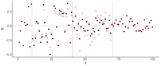
Figure 1: An example of how the data is transformed when we apply the transformation ๐‘ฟโ€ฒโ€‹(ฯ•)superscript๐‘ฟโ€ฒitalic-ฯ•\boldsymbol{X}^{\prime}(\phi). Here, the black points (filled circles) correspond to ๐‘ฟ๐‘ฟ\boldsymbol{X} and the red points (empty circles) to ๐‘ฟโ€ฒโ€‹(0.5)superscript๐‘ฟโ€ฒ0.5\boldsymbol{X}^{\prime}(0.5). Since ฯ•oโ€‹bโ€‹s>0.5subscriptitalic-ฯ•๐‘œ๐‘๐‘ 0.5\phi_{obs}>0.5 in this case, the points before ฯ„^^๐œ\hat{\tau} (shown by the dashed red line) are pulled in towards 0, and the points after the changepoint move away from 0. The overall sum of squares in the region {ฯ„^โˆ’h+1,โ€ฆ,ฯ„^+h}^๐œโ„Ž1โ€ฆ^๐œโ„Ž\{\hat{\tau}-h+1,\ldots,\hat{\tau}+h\} remains constant.

To make explicit the dependence of ๐‘ฟ๐‘ฟ\boldsymbol{X} on ฯ•italic-ฯ•\phi, we consider a re-parameterization of {Xฯ„^โˆ’h+1,โ€ฆ,Xฯ„^+h}subscript๐‘‹^๐œโ„Ž1โ€ฆsubscript๐‘‹^๐œโ„Ž\{X_{\hat{\tau}-h+1},\ldots,X_{\hat{\tau}+h}\}. Let C02=C(ฯ„^โˆ’h+1):(ฯ„^+h)2superscriptsubscript๐ถ02superscriptsubscript๐ถ:^๐œโ„Ž1^๐œโ„Ž2C_{0}^{2}=C_{(\hat{\tau}-h+1):(\hat{\tau}+h)}^{2}, the sum of the square of the data in the region being tested, and let

Wil=C(ฯ„^โˆ’h+1):(ฯ„^โˆ’h+i)2C(ฯ„^โˆ’h+1):(ฯ„^โˆ’h+i+1)2,i=1,โ€ฆ,hโˆ’1;Wir=C(ฯ„^+1):(ฯ„^+1)2C(ฯ„^+1):(ฯ„^+i+1)2,i=1,โ€ฆ,hโˆ’1.formulae-sequencesuperscriptsubscript๐‘Š๐‘–๐‘™superscriptsubscript๐ถ:^๐œโ„Ž1^๐œโ„Ž๐‘–2superscriptsubscript๐ถ:^๐œโ„Ž1^๐œโ„Ž๐‘–12formulae-sequence๐‘–1โ€ฆโ„Ž1formulae-sequencesuperscriptsubscript๐‘Š๐‘–๐‘Ÿsuperscriptsubscript๐ถ:^๐œ1^๐œ12superscriptsubscript๐ถ:^๐œ1^๐œ๐‘–12๐‘–1โ€ฆโ„Ž1\begin{split}W_{i}^{l}&=\frac{C_{(\hat{\tau}-h+1):(\hat{\tau}-h+i)}^{2}}{C_{(\hat{\tau}-h+1):(\hat{\tau}-h+i+1)}^{2}},~{}~{}i=1,\ldots,h-1;\\ W_{i}^{r}&=\frac{C_{(\hat{\tau}+1):(\hat{\tau}+1)}^{2}}{C_{(\hat{\tau}+1):(\hat{\tau}+i+1)}^{2}},~{}~{}i=1,\ldots,h-1.\end{split}

The following results shows how we can write the square of {Xฯ„^โˆ’h+1,โ€ฆ,Xฯ„^+h}subscript๐‘‹^๐œโ„Ž1โ€ฆsubscript๐‘‹^๐œโ„Ž\{X_{\hat{\tau}-h+1},\ldots,X_{\hat{\tau}+h}\} in terms of ฯ•italic-ฯ•\phi, C02subscriptsuperscript๐ถ20C^{2}_{0}, and Wkrsubscriptsuperscript๐‘Š๐‘Ÿ๐‘˜W^{r}_{k} and Wklsubscriptsuperscript๐‘Š๐‘™๐‘˜W^{l}_{k} for k=1,โ€ฆ,hโˆ’1๐‘˜1โ€ฆโ„Ž1k=1,\ldots,h-1, and that the latter set of variables are independent under the null hypothesis.

Lemma 1

We can write each Xtsubscript๐‘‹๐‘กX_{t}, for t=ฯ„^โˆ’h+1,โ€ฆ,ฯ„^+h๐‘ก^๐œโ„Ž1โ€ฆ^๐œโ„Žt=\hat{\tau}-h+1,\ldots,\hat{\tau}+h, in terms of W1l,โ€ฆ,Whโˆ’1lsuperscriptsubscript๐‘Š1๐‘™โ€ฆsuperscriptsubscript๐‘Šโ„Ž1๐‘™W_{1}^{l},\ldots,W_{h-1}^{l}, W1r,โ€ฆ,Whโˆ’1rsuperscriptsubscript๐‘Š1๐‘Ÿโ€ฆsuperscriptsubscript๐‘Šโ„Ž1๐‘ŸW_{1}^{r},\ldots,W_{h-1}^{r}, ฯ•italic-ฯ•\phi, and C02superscriptsubscript๐ถ02C_{0}^{2}. More specifically, for i=1,โ€ฆ,h๐‘–1โ€ฆโ„Ži=1,\ldots,h, we can write

Xฯ„^โˆ’h+i2={(1โˆ’Wiโˆ’1l)โ€‹โˆk=ihโˆ’1Wklโ€‹C02โ€‹ฯ•i=1,โ€ฆ,hโˆ’1(1โˆ’Wiโˆ’1l)โ€‹C02โ€‹ฯ•i=hXฯ„^+i2={(1โˆ’Wiโˆ’1r)โ€‹โˆk=ihโˆ’1Wkrโ€‹C02โ€‹(1โˆ’ฯ•)i=1,โ€ฆ,hโˆ’1(1โˆ’Wiโˆ’1r)โ€‹C02โ€‹(1โˆ’ฯ•)i=h,superscriptsubscript๐‘‹^๐œโ„Ž๐‘–2cases1superscriptsubscript๐‘Š๐‘–1๐‘™superscriptsubscriptproduct๐‘˜๐‘–โ„Ž1superscriptsubscript๐‘Š๐‘˜๐‘™superscriptsubscript๐ถ02italic-ฯ•๐‘–1โ€ฆโ„Ž11superscriptsubscript๐‘Š๐‘–1๐‘™superscriptsubscript๐ถ02italic-ฯ•๐‘–โ„Žsuperscriptsubscript๐‘‹^๐œ๐‘–2cases1superscriptsubscript๐‘Š๐‘–1๐‘Ÿsuperscriptsubscriptproduct๐‘˜๐‘–โ„Ž1superscriptsubscript๐‘Š๐‘˜๐‘Ÿsuperscriptsubscript๐ถ021italic-ฯ•๐‘–1โ€ฆโ„Ž11superscriptsubscript๐‘Š๐‘–1๐‘Ÿsuperscriptsubscript๐ถ021italic-ฯ•๐‘–โ„Ž\begin{split}X_{\hat{\tau}-h+i}^{2}&=\begin{cases}(1-W_{i-1}^{l})\prod_{k=i}^{h-1}W_{k}^{l}C_{0}^{2}\phi&i=1,\ldots,h-1\\ (1-W_{i-1}^{l})C_{0}^{2}\phi&i=h\end{cases}\\ X_{\hat{\tau}+i}^{2}&=\begin{cases}(1-W_{i-1}^{r})\prod_{k=i}^{h-1}W_{k}^{r}C_{0}^{2}(1-\phi)&i=1,\ldots,h-1\\ (1-W_{i-1}^{r})C_{0}^{2}(1-\phi)&i=h,\end{cases}\end{split} (4)

where for convenience we set W0l=W0r=0superscriptsubscript๐‘Š0๐‘™superscriptsubscript๐‘Š0๐‘Ÿ0W_{0}^{l}=W_{0}^{r}=0.

Lemma 2

Under H0subscript๐ป0H_{0}, W1l,โ€ฆ,Whโˆ’1l,W1r,โ€ฆ,Whโˆ’1r,ฯ•,C02superscriptsubscript๐‘Š1๐‘™โ€ฆsuperscriptsubscript๐‘Šโ„Ž1๐‘™superscriptsubscript๐‘Š1๐‘Ÿโ€ฆsuperscriptsubscript๐‘Šโ„Ž1๐‘Ÿitalic-ฯ•superscriptsubscript๐ถ02W_{1}^{l},\ldots,W_{h-1}^{l},W_{1}^{r},\ldots,W_{h-1}^{r},\phi,C_{0}^{2} are all independent.

Lemma 1 is easily verified. The proof of Lemma 2 is given in the supplementary material.

Therefore, conditioning on the dimensions of the data which are orthogonal to ฯ•italic-ฯ•\phi is equivalent to conditioning on the values of W1l,โ€ฆ,Whโˆ’1lsuperscriptsubscript๐‘Š1๐‘™โ€ฆsuperscriptsubscript๐‘Šโ„Ž1๐‘™W_{1}^{l},\ldots,W_{h-1}^{l}, W1r,โ€ฆ,Whโˆ’1rsuperscriptsubscript๐‘Š1๐‘Ÿโ€ฆsuperscriptsubscript๐‘Šโ„Ž1๐‘ŸW_{1}^{r},\ldots,W_{h-1}^{r}, and C02superscriptsubscript๐ถ02C_{0}^{2}. We can see from (4) above that doing this while allowing only ฯ•italic-ฯ•\phi to change has the effect of multiplying Xฯ„^โˆ’h+1,โ€ฆ,Xฯ„^subscript๐‘‹^๐œโ„Ž1โ€ฆsubscript๐‘‹^๐œX_{\hat{\tau}-h+1,\ldots,X_{\hat{\tau}}} by ฯ•ฯ•oโ€‹bโ€‹sitalic-ฯ•subscriptitalic-ฯ•๐‘œ๐‘๐‘ \sqrt{\frac{\phi}{\phi_{obs}}} and multiplying Xฯ„^+1,โ€ฆ,Xฯ„^+hsubscript๐‘‹^๐œ1โ€ฆsubscript๐‘‹^๐œโ„ŽX_{\hat{\tau}+1},\ldots,X_{\hat{\tau}+h} by 1โˆ’ฯ•1โˆ’ฯ•oโ€‹bโ€‹s1italic-ฯ•1subscriptitalic-ฯ•๐‘œ๐‘๐‘ \sqrt{\frac{1-\phi}{1-\phi_{obs}}}. (This transformation is illustrated in Figure 1.) Hence, let

Xtโ€ฒโ€‹(ฯ•)={Xttโ‰คฯ„^โˆ’hโ€‹ย orย โ€‹tโ‰ฅฯ„^+h+1ฯ•ฯ•oโ€‹bโ€‹sโ€‹Xtฯ„^โˆ’h+1โ‰คtโ‰คฯ„^1โˆ’ฯ•1โˆ’ฯ•oโ€‹bโ€‹sโ€‹Xtฯ„^+1โ‰คtโ‰คฯ„^+h.superscriptsubscript๐‘‹๐‘กโ€ฒitalic-ฯ•casessubscript๐‘‹๐‘ก๐‘ก^๐œโ„Žย orย ๐‘ก^๐œโ„Ž1italic-ฯ•subscriptitalic-ฯ•๐‘œ๐‘๐‘ subscript๐‘‹๐‘ก^๐œโ„Ž1๐‘ก^๐œ1italic-ฯ•1subscriptitalic-ฯ•๐‘œ๐‘๐‘ subscript๐‘‹๐‘ก^๐œ1๐‘ก^๐œโ„ŽX_{t}^{\prime}(\phi)=\begin{cases}X_{t}&t\leq\hat{\tau}-h\text{ or }t\geq\hat{\tau}+h+1\\ \sqrt{\frac{\phi}{\phi_{obs}}}X_{t}&\hat{\tau}-h+1\leq t\leq\hat{\tau}\\ \sqrt{\frac{1-\phi}{1-\phi_{obs}}}X_{t}&\hat{\tau}+1\leq t\leq\hat{\tau}+h.\end{cases} (5)

We consider only the subset of possible data sets {๐‘ฟโ€ฒโ€‹(ฯ•):ฯ•โˆˆโ„}conditional-setsuperscript๐‘ฟโ€ฒitalic-ฯ•italic-ฯ•โ„\{\boldsymbol{X}^{\prime}(\phi):\phi\in\mathbb{R}\}. Letting ๐’ฎ๐’ฎ\mathcal{S} denote the set ๐’ฎ={ฯ•:ฯ„^โˆˆโ„ณโ€‹(๐‘ฟโ€ฒโ€‹(ฯ•))}๐’ฎconditional-setitalic-ฯ•^๐œโ„ณsuperscript๐‘ฟโ€ฒitalic-ฯ•\mathcal{S}=\{\phi:\hat{\tau}\in\mathcal{M}(\boldsymbol{X}^{\prime}(\phi))\}, the post-selection p๐‘p-value we want to calculate is

p=Prโก(ฯ•โ‰คฯ•lโ€‹oโ€‹wโ€‹eโ€‹rโ€‹ย orย โ€‹ฯ•โ‰ฅฯ•uโ€‹pโ€‹pโ€‹eโ€‹r|ฯ•โˆˆ๐’ฎ).๐‘Pritalic-ฯ•subscriptitalic-ฯ•๐‘™๐‘œ๐‘ค๐‘’๐‘Ÿย orย italic-ฯ•conditionalsubscriptitalic-ฯ•๐‘ข๐‘๐‘๐‘’๐‘Ÿitalic-ฯ•๐’ฎp=\Pr\left(\phi\leq\phi_{lower}\text{ or }\phi\geq\phi_{upper}~{}|~{}\phi\in\mathcal{S}\right). (6)

Since we know that, under H0subscript๐ป0H_{0}, ฯ•โˆผBetaโ€‹(h2,h2)similar-toitalic-ฯ•Betaโ„Ž2โ„Ž2\phi\sim\text{Beta}\left(\frac{h}{2},\frac{h}{2}\right), the conditional distribution of ฯ•|ฯ•โˆˆ๐’ฎconditionalitalic-ฯ•italic-ฯ•๐’ฎ\phi|\phi\in\mathcal{S} is Betaโ€‹(h2,h2)Betaโ„Ž2โ„Ž2\text{Beta}\left(\frac{h}{2},\frac{h}{2}\right) truncated to ๐’ฎ๐’ฎ\mathcal{S}. Hence, calculating p๐‘p depends on calculating ๐’ฎ๐’ฎ\mathcal{S}. Calculation of ๐’ฎ๐’ฎ\mathcal{S} depends on the method used to estimate changepoints. In the following sections we describe how to do this for two classes of methods: in Section 3.1, we cover approaches based on finding changes in mean in Xt2superscriptsubscript๐‘‹๐‘ก2X_{t}^{2} using cumulative sums of squares, whilst in Section 3.2 we develop a more general approach, focusing on changepoint detection methods which attempt to maximize the likelihood ratio statistic.

3 Methods

3.1 CUSUM for change in variance

As a reminder, our model is

Xt=ฮผ+ฯƒtโ€‹ฯตt,t=1,โ€ฆ,T,formulae-sequencesubscript๐‘‹๐‘ก๐œ‡subscript๐œŽ๐‘กsubscriptitalic-ฯต๐‘ก๐‘ก1โ€ฆ๐‘‡X_{t}=\mu+\sigma_{t}\epsilon_{t},~{}~{}t=1,\ldots,T,

where ฯตtโˆผNโ€‹(0,1)similar-tosubscriptitalic-ฯต๐‘ก๐‘01\epsilon_{t}\sim N(0,1), and we assume that ฮผ๐œ‡\mu is known. Suppose, without loss of generality, that ฮผ=0๐œ‡0\mu=0 (if this is not the case, we can just replace Xtsubscript๐‘‹๐‘กX_{t} with Xtโˆ’ฮผsubscript๐‘‹๐‘ก๐œ‡X_{t}-\mu). Then a change in variance in ๐‘ฟ๐‘ฟ\boldsymbol{X} will correspond to a change in mean in ๐‘ฟ2superscript๐‘ฟ2\boldsymbol{X}^{2}. Therefore, one approach to detecting a change in variance in ๐‘ฟ๐‘ฟ\boldsymbol{X} is to look for a change in mean in ๐’€=๐‘ฟ2๐’€superscript๐‘ฟ2\boldsymbol{Y}=\boldsymbol{X}^{2}, for example by maximizing the cumulative sum (CUSUM) statistic, which is defined on a interval (s,e)={t:sโ‰คtโ‰คe}๐‘ ๐‘’conditional-set๐‘ก๐‘ ๐‘ก๐‘’(s,e)=\{t:s\leq t\leq e\} as

Gs,eโ€‹(t)=(tโˆ’s+1)โ€‹(eโˆ’t)eโˆ’s+1โ€‹(Yยฏs:tโˆ’Yยฏ(t+1):e),t=s,โ€ฆ,eโˆ’1.formulae-sequencesubscript๐บ๐‘ ๐‘’๐‘ก๐‘ก๐‘ 1๐‘’๐‘ก๐‘’๐‘ 1subscriptยฏ๐‘Œ:๐‘ ๐‘กsubscriptยฏ๐‘Œ:๐‘ก1๐‘’๐‘ก๐‘ โ€ฆ๐‘’1G_{s,e}(t)=\sqrt{\frac{(t-s+1)(e-t)}{e-s+1}}\left(\bar{Y}_{s:t}-\bar{Y}_{(t+1):e}\right),~{}~{}t=s,\ldots,e-1.

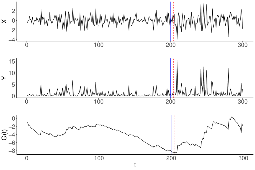
Figure 2 illustrates this process for a single changepoint. We will focus on using the CUSUM statistic with binary segmentation [35]; our approach to calculating p๐‘p-values will also extend to variants of this such as wild binary segmentation, as well as to the iterated cumulative sums of squares method of [19], which uses a different statistic based on the cumulative sums of squares.

To detect whether there is a change in mean in an interval (s,e)๐‘ ๐‘’(s,e), where 1โ‰คs<eโ‰คT1๐‘ ๐‘’๐‘‡1\leq s<e\leq T, we take

ฯ„^=argโ€‹maxtโก|Gs,eโ€‹(t)|,^๐œsubscriptargmax๐‘กsubscript๐บ๐‘ ๐‘’๐‘ก\hat{\tau}=\operatorname*{arg\,max}_{t}|G_{s,e}(t)|,

and determine that there is a changepoint at ฯ„^^๐œ\hat{\tau} if |Gs,eโ€‹(ฯ„^)|subscript๐บ๐‘ ๐‘’^๐œ|G_{s,e}(\hat{\tau})| is greater than some threshold. To detect multiple changepoints using binary segmentation, we start by maximizing |G1,Tโ€‹(t)|subscript๐บ1๐‘‡๐‘ก|G_{1,T}(t)| across the whole dataset; we then split the data at ฯ„^^๐œ\hat{\tau} and search for changepoints using Gs,eโ€‹(t)subscript๐บ๐‘ ๐‘’๐‘กG_{s,e}(t) calculated on each segment. This process is repeated until no more changepoints are detected.

Using this approach to detecting changes in variance is not always optimal, as the CUSUM statistic is derived under the assumption that the data follows a normal distribution with constant variance, which is not the case for our ๐’€๐’€\boldsymbol{Y}: when the variance of ๐‘ฟ๐‘ฟ\boldsymbol{X} changes, the variance of ๐’€๐’€\boldsymbol{Y} will also change. This leads to a higher false discovery rate in regions of higher variance, and a tendency to miss changepoints in less variable regions. However, it can still work well when the changes in variance are not too large. It also gives us the advantage of being able to adapt existing post-selection inference methods for the change in mean model, as we shall see in the next section.
Refer to caption
Figure 2: A simulated dataset with one change in variance. The data are simulated from Nโ€‹(0,1)๐‘01N(0,1) for t=1,โ€ฆ,200๐‘ก1โ€ฆ200t=1,\ldots,200 and from Nโ€‹(0,1.7)๐‘01.7N(0,1.7) for t=201,โ€ฆ,300๐‘ก201โ€ฆ300t=201,\ldots,300. The blue line shows the true changepoint location and the dashed red line the changepoint location estimated by maximizing |G1,Tโ€‹(t)|subscript๐บ1๐‘‡๐‘ก|G_{1,T}(t)|.

3.1.1 Calculating the post-selection p๐‘p-value

To calculate the p๐‘p-value in (6), we must compute ๐’ฎ={ฯ•:ฯ„^โˆˆโ„ณโ€‹(๐‘ฟโ€ฒโ€‹(ฯ•))}๐’ฎconditional-setitalic-ฯ•^๐œโ„ณsuperscript๐‘ฟโ€ฒitalic-ฯ•\mathcal{S}=\{\phi:\hat{\tau}\in\mathcal{M}(\boldsymbol{X}^{\prime}(\phi))\} โ€“ in other words, we need to find the set of ฯ•italic-ฯ•\phi values such that our changepoint algorithm detects a changepoint at ฯ„^^๐œ\hat{\tau}. ๐’ฎ๐’ฎ\mathcal{S} is therefore dependent on our choice of changepoint algorithm. We will focus initially on binary segmentation; the method generalizes straightforwardly to other related algorithms.

To calculate ๐’ฎ๐’ฎ\mathcal{S} we can borrow ideas from methods used for the change in mean model. [18] showed that by conditioning on the set of changes โ„ณโ€‹(๐‘ฟ)โ„ณ๐‘ฟ\mathcal{M}(\boldsymbol{X}), the order in which the changes are found, and the direction of each change (positive or negative), we can write down a set of inequalities which must be satisfied by the CUSUM statistic. For a given segment (s,e)๐‘ ๐‘’(s,e), in order to detect a change point at ฯ„^^๐œ\hat{\tau} we must have |Gs,eโ€‹(ฯ„^)|โ‰ฅฮปsubscript๐บ๐‘ ๐‘’^๐œ๐œ†|G_{s,e}(\hat{\tau})|\geq\lambda, where ฮป๐œ†\lambda is the changepoint detection threshold, and

{(โˆ’d^)โ‹…Gs,eโ€‹(ฯ„^)>Gs,eโ€‹(t)(โˆ’d^)โ‹…Gs,eโ€‹(ฯ„^)>โˆ’Gs,eโ€‹(t)โ€‹forย โ€‹t=s,โ€ฆ,eโˆ’1;tโ‰ ฯ„^,formulae-sequencecasesโ‹…^๐‘‘subscript๐บ๐‘ ๐‘’^๐œsubscript๐บ๐‘ ๐‘’๐‘กotherwiseโ‹…^๐‘‘subscript๐บ๐‘ ๐‘’^๐œsubscript๐บ๐‘ ๐‘’๐‘กotherwiseforย ๐‘ก๐‘ โ€ฆ๐‘’1๐‘ก^๐œ\begin{cases}(-\hat{d})\cdot G_{s,e}(\hat{\tau})>G_{s,e}(t)\\ (-\hat{d})\cdot G_{s,e}(\hat{\tau})>-G_{s,e}(t)\end{cases}\text{for }t=s,\ldots,e-1;t\neq\hat{\tau},

where d^โˆˆ{+1,โˆ’1}^๐‘‘11\hat{d}\in\{+1,-1\} is the direction of the change. For no changepoint to be detected in the interval (s,e)๐‘ ๐‘’(s,e), we must have

{Gs,eโ€‹(t)<ฮปGs,eโ€‹(t)>โˆ’ฮปโ€‹forย โ€‹t=s,โ€ฆ,eโˆ’1casessubscript๐บ๐‘ ๐‘’๐‘ก๐œ†otherwisesubscript๐บ๐‘ ๐‘’๐‘ก๐œ†otherwiseforย ๐‘ก๐‘ โ€ฆ๐‘’1\begin{cases}G_{s,e}(t)<\lambda\\ G_{s,e}(t)>-\lambda\end{cases}\text{for }t=s,\ldots,e-1

Hence, we can write down a set of linear inequalities in the data for each iteration of binary segmentation, which must all be satisfied for the particular set of changepoints, with the order and directions of change, to be found. For the change in mean model, the test statistic is defined as ฯ•=๐‚โŠคโ€‹๐‘ฟitalic-ฯ•superscript๐‚top๐‘ฟ\phi=\boldsymbol{\nu}^{\top}\boldsymbol{X}, where

ฮฝt={0tโ‰คฯ„^โˆ’h1hฯ„^โˆ’h+1โ‰คtโ‰คฯ„^โˆ’1hฯ„^+1โ‰คtโ‰คฯ„^+h0tโ‰ฅฯ„^+h+1.subscript๐œˆ๐‘กcases0๐‘ก^๐œโ„Ž1โ„Ž^๐œโ„Ž1๐‘ก^๐œ1โ„Ž^๐œ1๐‘ก^๐œโ„Ž0๐‘ก^๐œโ„Ž1\nu_{t}=\begin{cases}0&t\leq\hat{\tau}-h\\ \frac{1}{h}&\hat{\tau}-h+1\leq t\leq\hat{\tau}\\ -\frac{1}{h}&\hat{\tau}+1\leq t\leq\hat{\tau}+h\\ 0&t\geq\hat{\tau}+h+1.\end{cases}

As for our model, we can then introduce perturbations of the data that correspond to changes in ฯ•italic-ฯ•\phi whilst fixing the information orthogonal to ฯ•italic-ฯ•\phi:

๐‘ฟโ€ฒโ€‹(ฯ•)=๐‘ฟoโ€‹bโ€‹sโˆ’๐‚โ€–๐‚โ€–22โ€‹ฯ•oโ€‹bโ€‹s+๐‚โ€–๐‚โ€–22โ€‹ฯ•.superscript๐‘ฟโ€ฒitalic-ฯ•subscript๐‘ฟ๐‘œ๐‘๐‘ ๐‚superscriptsubscriptnorm๐‚22subscriptitalic-ฯ•๐‘œ๐‘๐‘ ๐‚superscriptsubscriptnorm๐‚22italic-ฯ•\boldsymbol{X}^{\prime}(\phi)=\boldsymbol{X}_{obs}-\frac{\boldsymbol{\nu}}{||\boldsymbol{\nu}||_{2}^{2}}\phi_{obs}+\frac{\boldsymbol{\nu}}{||\boldsymbol{\nu}||_{2}^{2}}\phi.

Since Gs,eโ€‹(t)subscript๐บ๐‘ ๐‘’๐‘กG_{s,e}(t) is a linear function of ๐‘ฟ๐‘ฟ\boldsymbol{X}, and ๐‘ฟโ€ฒโ€‹(ฯ•)superscript๐‘ฟโ€ฒitalic-ฯ•\boldsymbol{X}^{\prime}(\phi) is a linear function of ฯ•italic-ฯ•\phi, the CUSUM statistic in terms of ฯ•italic-ฯ•\phi is also linear in ฯ•italic-ฯ•\phi. Hence, we can write the set of inequalities in Gs,eโ€‹(t)subscript๐บ๐‘ ๐‘’๐‘กG_{s,e}(t) as linear inequalities in ฯ•italic-ฯ•\phi, and they will therefore hold for an interval of ฯ•italic-ฯ•\phi values, which it is straightforward to calculate. [20] shows that we can increase power by extending this idea to avoid conditioning on the order and directions of the changes, by calculating the intervals associated with each possible combination of changes which yield ฯ„^โˆˆโ„ณโ€‹(๐‘ฟ)^๐œโ„ณ๐‘ฟ\hat{\tau}\in\mathcal{M}(\boldsymbol{X}). This gives us the set ๐’ฎ๐’ฎ\mathcal{S} which is the union of all such intervals.

For the change in variance model, we can use the same approach, as the inequalities we write down in terms of Gs,eโ€‹(t)subscript๐บ๐‘ ๐‘’๐‘กG_{s,e}(t) are the same. As a reminder, the CUSUM statistic is

Gs,eโ€‹(t)=((tโˆ’s+1)โ€‹(eโˆ’t)eโˆ’s+1)1/2โ€‹(Yยฏs:tโˆ’Yยฏ(t+1):e)=((tโˆ’s+1)โ€‹(eโˆ’t)eโˆ’s+1)1/2โ€‹(1tโˆ’s+1โ€‹โˆ‘j=stXj2โˆ’1eโˆ’tโ€‹โˆ‘j=t+1eXj2),subscript๐บ๐‘ ๐‘’๐‘กsuperscript๐‘ก๐‘ 1๐‘’๐‘ก๐‘’๐‘ 112subscriptยฏ๐‘Œ:๐‘ ๐‘กsubscriptยฏ๐‘Œ:๐‘ก1๐‘’superscript๐‘ก๐‘ 1๐‘’๐‘ก๐‘’๐‘ 1121๐‘ก๐‘ 1superscriptsubscript๐‘—๐‘ ๐‘กsuperscriptsubscript๐‘‹๐‘—21๐‘’๐‘กsuperscriptsubscript๐‘—๐‘ก1๐‘’superscriptsubscript๐‘‹๐‘—2\begin{split}G_{s,e}(t)&=\left(\frac{(t-s+1)(e-t)}{e-s+1}\right)^{1/2}\left(\bar{Y}_{s:t}-\bar{Y}_{(t+1):e}\right)\\ &=\left(\frac{(t-s+1)(e-t)}{e-s+1}\right)^{1/2}\left(\frac{1}{t-s+1}\sum_{j=s}^{t}X_{j}^{2}-\frac{1}{e-t}\sum_{j=t+1}^{e}X_{j}^{2}\right),\end{split}

so

Gs,eโ€‹(ฯ•,t)=((tโˆ’s+1)โ€‹(eโˆ’t)eโˆ’s+1)1/2โ€‹(1tโˆ’s+1โ€‹โˆ‘j=stXjโ€ฒโ€‹(ฯ•)2โˆ’1eโˆ’tโ€‹โˆ‘j=t+1eXjโ€ฒโ€‹(ฯ•)2)subscript๐บ๐‘ ๐‘’italic-ฯ•๐‘กsuperscript๐‘ก๐‘ 1๐‘’๐‘ก๐‘’๐‘ 1121๐‘ก๐‘ 1superscriptsubscript๐‘—๐‘ ๐‘กsuperscriptsubscript๐‘‹๐‘—โ€ฒsuperscriptitalic-ฯ•21๐‘’๐‘กsuperscriptsubscript๐‘—๐‘ก1๐‘’superscriptsubscript๐‘‹๐‘—โ€ฒsuperscriptitalic-ฯ•2G_{s,e}(\phi,t)=\left(\frac{(t-s+1)(e-t)}{e-s+1}\right)^{1/2}\left(\frac{1}{t-s+1}\sum_{j=s}^{t}X_{j}^{\prime}(\phi)^{2}-\frac{1}{e-t}\sum_{j=t+1}^{e}X_{j}^{\prime}(\phi)^{2}\right) (7)

Using the definition of ๐‘ฟโ€ฒโ€‹(ฯ•)superscript๐‘ฟโ€ฒitalic-ฯ•\boldsymbol{X}^{\prime}(\phi) from (5), we can write each element of this as Xjโ€ฒโ€‹(ฯ•)=aj+bjโ€‹ฯ•superscriptsubscript๐‘‹๐‘—โ€ฒitalic-ฯ•subscript๐‘Ž๐‘—subscript๐‘๐‘—italic-ฯ•X_{j}^{\prime}(\phi)=a_{j}+b_{j}\phi where

aj={Xj2ฯ•โ‰คฯ„^โˆ’hโ€‹ย orย โ€‹ฯ•>ฯ„^+h0ฯ„^โˆ’h<ฯ•โ‰คฯ„^11โˆ’ฯ•oโ€‹bโ€‹sโ€‹Xj2ฯ„^<ฯ•โ‰คฯ„^+hsubscript๐‘Ž๐‘—casessuperscriptsubscript๐‘‹๐‘—2italic-ฯ•^๐œโ„Žย orย italic-ฯ•^๐œโ„Ž0^๐œโ„Žitalic-ฯ•^๐œ11subscriptitalic-ฯ•๐‘œ๐‘๐‘ superscriptsubscript๐‘‹๐‘—2^๐œitalic-ฯ•^๐œโ„Ža_{j}=\begin{cases}X_{j}^{2}&\phi\leq\hat{\tau}-h\text{ or }\phi>\hat{\tau}+h\\ 0&\hat{\tau}-h<\phi\leq\hat{\tau}\\ \frac{1}{1-\phi_{obs}}X_{j}^{2}&\hat{\tau}<\phi\leq\hat{\tau}+h\end{cases}
bj={0ฯ•โ‰คฯ„^โˆ’hโ€‹ย orย โ€‹ฯ•>ฯ„^+h1ฯ•oโ€‹bโ€‹sโ€‹Xj2ฯ„^โˆ’h<ฯ•โ‰คฯ„^โˆ’11โˆ’ฯ•oโ€‹bโ€‹sโ€‹Xj2ฯ„^<ฯ•โ‰คฯ„^+hsubscript๐‘๐‘—cases0italic-ฯ•^๐œโ„Žย orย italic-ฯ•^๐œโ„Ž1subscriptitalic-ฯ•๐‘œ๐‘๐‘ superscriptsubscript๐‘‹๐‘—2^๐œโ„Žitalic-ฯ•^๐œ11subscriptitalic-ฯ•๐‘œ๐‘๐‘ superscriptsubscript๐‘‹๐‘—2^๐œitalic-ฯ•^๐œโ„Žb_{j}=\begin{cases}0&\phi\leq\hat{\tau}-h\text{ or }\phi>\hat{\tau}+h\\ \frac{1}{\phi_{obs}}X_{j}^{2}&\hat{\tau}-h<\phi\leq\hat{\tau}\\ -\frac{1}{1-\phi_{obs}}X_{j}^{2}&\hat{\tau}<\phi\leq\hat{\tau}+h\end{cases}

Hence, letting G0=((tโˆ’s+1)โ€‹(eโˆ’t)eโˆ’s+1)1/2subscript๐บ0superscript๐‘ก๐‘ 1๐‘’๐‘ก๐‘’๐‘ 112G_{0}=\left(\frac{(t-s+1)(e-t)}{e-s+1}\right)^{1/2}, we can write (7) as

Gs,eโ€‹(ฯ•,t)=G0โ€‹(1tโˆ’s+1โ€‹โˆ‘j=st(aj+bj)โ€‹ฯ•โˆ’1eโˆ’tโ€‹โˆ‘j=t+1e(aj+bj)โ€‹ฯ•)=G0โ€‹((1tโˆ’s+1โ€‹โˆ‘j=stajโˆ’1eโˆ’tโ€‹โˆ‘j=t+1eaj)+(1tโˆ’s+1โ€‹โˆ‘j=stbjโˆ’1eโˆ’tโ€‹โˆ‘j=t+1ebj)โ€‹ฯ•).subscript๐บ๐‘ ๐‘’italic-ฯ•๐‘กsubscript๐บ01๐‘ก๐‘ 1superscriptsubscript๐‘—๐‘ ๐‘กsubscript๐‘Ž๐‘—subscript๐‘๐‘—italic-ฯ•1๐‘’๐‘กsuperscriptsubscript๐‘—๐‘ก1๐‘’subscript๐‘Ž๐‘—subscript๐‘๐‘—italic-ฯ•subscript๐บ01๐‘ก๐‘ 1superscriptsubscript๐‘—๐‘ ๐‘กsubscript๐‘Ž๐‘—1๐‘’๐‘กsuperscriptsubscript๐‘—๐‘ก1๐‘’subscript๐‘Ž๐‘—1๐‘ก๐‘ 1superscriptsubscript๐‘—๐‘ ๐‘กsubscript๐‘๐‘—1๐‘’๐‘กsuperscriptsubscript๐‘—๐‘ก1๐‘’subscript๐‘๐‘—italic-ฯ•\begin{split}G_{s,e}(\phi,t)&=G_{0}\left(\frac{1}{t-s+1}\sum_{j=s}^{t}(a_{j}+b_{j})\phi-\frac{1}{e-t}\sum_{j=t+1}^{e}(a_{j}+b_{j})\phi\right)\\ &=G_{0}\left(\left(\frac{1}{t-s+1}\sum_{j=s}^{t}a_{j}-\frac{1}{e-t}\sum_{j=t+1}^{e}a_{j}\right)+\left(\frac{1}{t-s+1}\sum_{j=s}^{t}b_{j}-\frac{1}{e-t}\sum_{j=t+1}^{e}b_{j}\right)\phi\right).\end{split}

This is linear in ฯ•italic-ฯ•\phi, so we can once again compute each possible interval by resolving a set of linear inequalities in ฯ•italic-ฯ•\phi. We can use the method of [20] to efficiently compute ๐’ฎ๐’ฎ\mathcal{S} (and hence p๐‘p).

3.2 Likelihood-ratio based detection of changes
Refer to caption
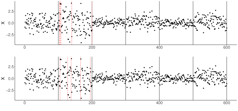
Figure 3: Estimating changepoints using binary segmentation and wild binary segmentation with the CUSUM statistic for a simulated data set with multiple changes. The solid black lines correspond to true changes, the dashed red lines to estimated changepoints. The method tends to over-estimate changepoints within the region of highest variance, whilst missing changes in other regions.

Whilst post-selection inference is relatively straightforward for the piecewise constant variance model when estimating changepoint locations using the CUSUM statistic, the use of the CUSUM statistic can lead to poor detection of changes. For example, Figure 3 shows an example of a simulated data set with 5 changepoints, where we apply binary segmentation and wild binary segmentation to detect changepoints. Both methods overestimate the number of changes in the region with highest variance, but fail to detect changes in other regions.

We can achieve more accurate changepoint detection by maximizing the likelihood ratio statistic, which on an interval (s,e)๐‘ ๐‘’(s,e) is defined as

ฮ›s,eโ€‹(ฯ„)=(sโˆ’e+1)โ€‹logโ€‹โˆ‘t=seXt2โˆ’(ฯ„โˆ’s+1)โ€‹logโ€‹โˆ‘t=sฯ„Xt2โˆ’(eโˆ’ฯ„)โ€‹logโ€‹โˆ‘t=ฯ„+1eXt2subscriptฮ›๐‘ ๐‘’๐œ๐‘ ๐‘’1superscriptsubscript๐‘ก๐‘ ๐‘’superscriptsubscript๐‘‹๐‘ก2๐œ๐‘ 1superscriptsubscript๐‘ก๐‘ ๐œsuperscriptsubscript๐‘‹๐‘ก2๐‘’๐œsuperscriptsubscript๐‘ก๐œ1๐‘’superscriptsubscript๐‘‹๐‘ก2\Lambda_{s,e}(\tau)=(s-e+1)\log\sum_{t=s}^{e}X_{t}^{2}-(\tau-s+1)\log\sum_{t=s}^{\tau}X_{t}^{2}-(e-\tau)\log\sum_{t=\tau+1}^{e}X_{t}^{2} (8)

To estimate a single changepoint, we calculate ฮ›1,Tโ€‹(ฯ„)subscriptฮ›1๐‘‡๐œ\Lambda_{1,T}(\tau) for ฯ„=1,โ€ฆ,Tโˆ’1๐œ1โ€ฆ๐‘‡1\tau=1,\ldots,T-1, and take ฯ„^=argโ€‹maxฯ„โกฮ›1,Tโ€‹(ฯ„)^๐œsubscriptargmax๐œsubscriptฮ›1๐‘‡๐œ\hat{\tau}=\operatorname*{arg\,max}_{\tau}\Lambda_{1,T}(\tau). For multiple changepoints, we can either use an iterative method such as binary segmentation, or a penalized likelihood method such as PELT [23]. The approach we develop below will apply in both cases.

Table 1: Proportion of runs in which binary segmentation detected a changepoint within 10 of each true changepoint, using CUSUM and likelihood ratio approaches.
CUSUM LRS
ฯ„=100๐œ100\tau=100 0.755 0.915
ฯ„=200๐œ200\tau=200 0.972 0.992
ฯ„=300๐œ300\tau=300 0.012 0.914

Table 1 demonstrates how this leads to increased accuracy compared with using the CUSUM statistic. We simulated data from a model with T=400๐‘‡400T=400 and 3 changepoints at ฯ„=100,200,300๐œ100200300\tau=100,200,300; the variances on the four segments being {1,4,0.25,1}140.251\{1,4,0.25,1\}, and for each simulated data set we used binary segmentation to estimate three changepoint locations, using both the CUSUM statistic and the likelihood ratio statistic to determine a change. The table records the proportion of runs in which a changepoint was detected within 10 of each true changepoint. We see that CUSUM does reasonably well at detecting the first two changes, but does very badly at locating the third, smaller change. Using the likelihood ratio statistic, however, all three changepoints are detected in over 90%percent9090\% of cases.

3.2.1 Post-selection inference

As a reminder, the post-selection p๐‘p-value we want to calculate is

Prโก(ฯ•โ‰คฯ•lโ€‹oโ€‹wโ€‹eโ€‹rโ€‹ย orย โ€‹ฯ•โ‰ฅฯ•uโ€‹pโ€‹pโ€‹eโ€‹r|ฯ•โˆˆ๐’ฎ),Pritalic-ฯ•subscriptitalic-ฯ•๐‘™๐‘œ๐‘ค๐‘’๐‘Ÿย orย italic-ฯ•conditionalsubscriptitalic-ฯ•๐‘ข๐‘๐‘๐‘’๐‘Ÿitalic-ฯ•๐’ฎ\Pr\left(\phi\leq\phi_{lower}\text{ or }\phi\geq\phi_{upper}~{}|~{}\phi\in\mathcal{S}\right),

where ๐’ฎ={ฯ•:ฯ„^โˆˆโ„ณโ€‹(๐‘ฟโ€ฒโ€‹(ฯ•))}๐’ฎconditional-setitalic-ฯ•^๐œโ„ณsuperscript๐‘ฟโ€ฒitalic-ฯ•\mathcal{S}=\{\phi:\hat{\tau}\in\mathcal{M}(\boldsymbol{X}^{\prime}(\phi))\}. Previously, when detecting changes based on the CUSUM statistic, we were able to write down a set of linear inequalities in ฯ•italic-ฯ•\phi which defined the set ๐’ฎ๐’ฎ\mathcal{S}. However, while we can write down inequalities in ฮ›s,eโ€‹(ฯ•,ฯ„)subscriptฮ›๐‘ ๐‘’italic-ฯ•๐œ\Lambda_{s,e}(\phi,\tau) as we did for Gs,eโ€‹(ฯ•,ฯ„)subscript๐บ๐‘ ๐‘’italic-ฯ•๐œG_{s,e}(\phi,\tau), ฮ›s,eโ€‹(ฯ•,ฯ„)subscriptฮ›๐‘ ๐‘’italic-ฯ•๐œ\Lambda_{s,e}(\phi,\tau) is not a linear function of ฯ•italic-ฯ•\phi: we can show that

ฮ›s,eโ€‹(ฯ„,ฯ•)=logโก((As,eโ€‹ฯ•+Bs,e)sโˆ’e+1(As,ฯ„โ€‹ฯ•+Bs,ฯ„)ฯ„โˆ’s+1โ€‹((As,eโˆ’As,ฯ„)โ€‹ฯ•+Bs,eโˆ’Bs,ฯ„)eโˆ’ฯ„),subscriptฮ›๐‘ ๐‘’๐œitalic-ฯ•superscriptsubscript๐ด๐‘ ๐‘’italic-ฯ•subscript๐ต๐‘ ๐‘’๐‘ ๐‘’1superscriptsubscript๐ด๐‘ ๐œitalic-ฯ•subscript๐ต๐‘ ๐œ๐œ๐‘ 1superscriptsubscript๐ด๐‘ ๐‘’subscript๐ด๐‘ ๐œitalic-ฯ•subscript๐ต๐‘ ๐‘’subscript๐ต๐‘ ๐œ๐‘’๐œ\Lambda_{s,e}(\tau,\phi)=\log\left(\frac{(A_{s,e}\phi+B_{s,e})^{s-e+1}}{(A_{s,\tau}\phi+B_{s,\tau})^{\tau-s+1}((A_{s,e}-A_{s,\tau})\phi+B_{s,e}-B_{s,\tau})^{e-\tau}}\right), (9)

where As,esubscript๐ด๐‘ ๐‘’A_{s,e} and Bs,esubscript๐ต๐‘ ๐‘’B_{s,e} are constants depending on s๐‘ s, e๐‘’e, hโ„Žh, and ฯ•oโ€‹bโ€‹ssubscriptitalic-ฯ•๐‘œ๐‘๐‘ \phi_{obs} (see the Appendix for more details). In general, it is not possible to analytically solve these inequalities for ฯ•italic-ฯ•\phi as it was earlier.

However ๐’ฎ๐’ฎ\mathcal{S} still consists of a union of intervals as the inequalities are smooth functions of ฯ•italic-ฯ•\phi. To illustrate this, Figure 4 shows a plot of ฮ›โ€‹(ฯ„,ฯ•)ฮ›๐œitalic-ฯ•\Lambda(\tau,\phi) against ฯ•italic-ฯ•\phi for a simulated data set for different values of ฯ„๐œ\tau; the red line corresponds to ฯ„^^๐œ\hat{\tau}. The values of ฯ•italic-ฯ•\phi which are in ๐’ฎ๐’ฎ\mathcal{S} are hence those for which the red line is higher than any of the other lines on the plot.

Refer to caption
Figure 4: Example plots of ฮ›ฮ›\Lambda against ฯ•italic-ฯ•\phi; each line corresponds to ฮ›โ€‹(ฯ„,ฯ•)ฮ›๐œitalic-ฯ•\Lambda(\tau,\phi) for a different value of ฯ„โˆˆ1,โ€ฆ,Tโˆ’1๐œ1โ€ฆ๐‘‡1\tau\in 1,\ldots,T-1. Each shaded region corresponds to a range of ฯ•italic-ฯ•\phi values where a different ฯ„๐œ\tau maximizes ฮ›โ€‹(ฯ„,ฯ•)ฮ›๐œitalic-ฯ•\Lambda(\tau,\phi).

Although we cannot compute ๐’ฎ๐’ฎ\mathcal{S} directly, we can find out whether a given ฯ•italic-ฯ•\phi is in ๐’ฎ๐’ฎ\mathcal{S} by computing ๐‘ฟโ€ฒโ€‹(ฯ•)superscript๐‘ฟโ€ฒitalic-ฯ•\boldsymbol{X}^{\prime}(\phi), as in (5), and re-running the changepoint algorithm to obtain the set of estimated changepoints โ„ณโ€‹(๐‘ฟโ€ฒโ€‹(ฯ•))โ„ณsuperscript๐‘ฟโ€ฒitalic-ฯ•\mathcal{M}(\boldsymbol{X}^{\prime}(\phi)). Hence, one way to approximate ๐’ฎ๐’ฎ\mathcal{S} is by randomly sampling ฯ•italic-ฯ•\phi values and calculating whether each is in ๐’ฎ๐’ฎ\mathcal{S}. We can then estimate p๐‘p by calculating what proportion of ฯ•italic-ฯ•\phi values which are in ๐’ฎ๐’ฎ\mathcal{S} are also in the critical region ๐’ž={ฯ•:ฯ•โ‰คฯ•lโ€‹oโ€‹wโ€‹eโ€‹rโ€‹ย orย โ€‹ฯ•โ‰ฅฯ•uโ€‹pโ€‹pโ€‹eโ€‹r}๐’žconditional-setitalic-ฯ•italic-ฯ•subscriptitalic-ฯ•๐‘™๐‘œ๐‘ค๐‘’๐‘Ÿย orย italic-ฯ•subscriptitalic-ฯ•๐‘ข๐‘๐‘๐‘’๐‘Ÿ\mathcal{C}=\{\phi:\phi\leq\phi_{lower}\text{ or }\phi\geq\phi_{upper}\}:

p^=โˆ‘i=1N๐•€{ฯ„^โˆˆโ„ณโ€‹(๐‘ฟโ€ฒโ€‹(ฯ•(i))),ฯ•(i)โˆˆ๐’ž}โˆ‘i=1N๐•€{ฯ„^โˆˆโ„ณโ€‹(๐‘ฟโ€ฒโ€‹(ฯ•(i)))}.^๐‘superscriptsubscript๐‘–1๐‘subscript๐•€formulae-sequence^๐œโ„ณsuperscript๐‘ฟโ€ฒsuperscriptitalic-ฯ•๐‘–superscriptitalic-ฯ•๐‘–๐’žsuperscriptsubscript๐‘–1๐‘subscript๐•€^๐œโ„ณsuperscript๐‘ฟโ€ฒsuperscriptitalic-ฯ•๐‘–\hat{p}=\frac{\sum_{i=1}^{N}\mathbb{I}_{\{\hat{\tau}\in\mathcal{M}(\boldsymbol{X}^{\prime}(\phi^{(i)})),~{}~{}\phi^{(i)}\in\mathcal{C}\}}}{\sum_{i=1}^{N}\mathbb{I}_{\{\hat{\tau}\in\mathcal{M}(\boldsymbol{X}^{\prime}(\phi^{(i)}))\}}}. (10)

However, sampling ฯ•italic-ฯ•\phi from its unconditional distribution Betaโ€‹(h2,h2)Betaโ„Ž2โ„Ž2\text{Beta}\left(\frac{h}{2},\frac{h}{2}\right) often leads to very slow convergence of p^^๐‘\hat{p}, as Prโก(ฯ•โˆˆ๐’ฎ)Pritalic-ฯ•๐’ฎ\Pr(\phi\in\mathcal{S}) is typically small, so only a small proportion of samples will contribute to p^^๐‘\hat{p}: the rest are discarded.

Since sampling in this way requires re-applying the changepoint algorithm for each ฯ•(i)superscriptitalic-ฯ•๐‘–\phi^{(i)}, which may be computationally demanding (the length of time taken to apply the algorithm will scale with the number of data points and the number of detected changes), using a large number of samples to estimate the p๐‘p-value is undesirable. We therefore want to find ways to reduce the number of samples necessary to get a good p๐‘p-value estimate p^^๐‘\hat{p}.

One way to reduce the variance of p^^๐‘\hat{p}, without increasing the computation time, is to use stratified sampling. For i=1,โ€ฆ,N๐‘–1โ€ฆ๐‘i=1,\ldots,N, we sample z(i)โˆผUโ€‹(iโˆ’1N,iN)similar-tosuperscript๐‘ง๐‘–๐‘ˆ๐‘–1๐‘๐‘–๐‘z^{(i)}\sim U(\frac{i-1}{N},\frac{i}{N}). We then calculate ฯ•(i)superscriptitalic-ฯ•๐‘–\phi^{(i)} to satisfy Prโก(ฯ•<ฯ•(i))=z(i)Pritalic-ฯ•superscriptitalic-ฯ•๐‘–superscript๐‘ง๐‘–\Pr(\phi<\phi^{(i)})=z^{(i)}. (Section C.2 in the supplementary material shows how the variance of p^^๐‘\hat{p} decreases using stratified, compared to random sampling.) Doing this ensures that our set of sampled ฯ•italic-ฯ•\phi values are spread evenly across the sample space, which can help to give more accurate estimates. However, it is not infrequently the case that Prโก(ฯ•โˆˆ๐’ฎ)Pritalic-ฯ•๐’ฎ\Pr(\phi\in\mathcal{S}) is of the order of 1N1๐‘\frac{1}{N} or smaller, in which case using stratified sampling is unlikely to significantly improve the estimate p^^๐‘\hat{p}, as we will still have very few ฯ•(i)โˆˆ๐’ฎsuperscriptitalic-ฯ•๐‘–๐’ฎ\phi^{(i)}\in\mathcal{S}.

To overcome this we resort to using simulation to estimate the intervals that contribute to ๐’ฎ๐’ฎ\mathcal{S}. These estimates can then be used to directly estimate the post-selection p๐‘p-value or to construct better proposal distributions for an importance sampling based Monte Carlo approach.

3.2.2 Estimating ๐’ฎ๐’ฎ\mathcal{S} using Gaussian processes

If we can calculate ๐’ฎ๐’ฎ\mathcal{S} then it is straightforward to calculate the p๐‘p-value. Whilst ๐’ฎ๐’ฎ\mathcal{S} is intractable, as mentioned above, for any value of ฯ•italic-ฯ•\phi we can calculate ๐•€ฯ•โˆˆ๐’ฎsubscript๐•€italic-ฯ•๐’ฎ\mathbb{I}_{\phi\in\mathcal{S}}. We can represent our beliefs about ๐•€ฯ•โˆˆ๐’ฎsubscript๐•€italic-ฯ•๐’ฎ\mathbb{I}_{\phi\in\mathcal{S}} as a function of ฯ•italic-ฯ•\phi, through a probability distribution pโ€‹(ฯ•)=Prโก(๐•€ฯ•โˆˆ๐’ฎ)๐‘italic-ฯ•Prsubscript๐•€italic-ฯ•๐’ฎp(\phi)=\Pr(\mathbb{I}_{\phi\in\mathcal{S}}) that gives a probability to ๐•€ฯ•โˆˆ๐’ฎsubscript๐•€italic-ฯ•๐’ฎ\mathbb{I}_{\phi\in\mathcal{S}} for each ฯ•โˆˆ[0,1]italic-ฯ•01\phi\in[0,1]. We can then model this function as a Gaussian process (GP) (see e.g. [37]). This means that we treat pโ€‹(ฯ•)๐‘italic-ฯ•p(\phi) as a random function such that for any set of ฯ•italic-ฯ•\phi values, {ฯ•1,โ€ฆ,ฯ•N}subscriptitalic-ฯ•1โ€ฆsubscriptitalic-ฯ•๐‘\{\phi_{1},\ldots,\phi_{N}\}, (pโ€‹(ฯ•1),โ€ฆ,pโ€‹(ฯ•N))๐‘subscriptitalic-ฯ•1โ€ฆ๐‘subscriptitalic-ฯ•๐‘\left(p(\phi_{1}),\ldots,p(\phi_{N})\right) follows a multivariate Gaussian distribution. We can then take as our estimate, Prโก(๐•€ฯ•โˆˆ๐’ฎ)Prsubscript๐•€italic-ฯ•๐’ฎ\Pr(\mathbb{I}_{\phi\in\mathcal{S}}), the mean of the Gaussian process. Given an observation ฯ•โˆˆ๐’ฎitalic-ฯ•๐’ฎ\phi\in\mathcal{S} or ฯ•โˆ‰๐’ฎitalic-ฯ•๐’ฎ\phi\notin\mathcal{S}, the GP will force pโ€‹(ฯ•)๐‘italic-ฯ•p(\phi) to take the value either 0 or 1. In between, the mean of the Gaussian process will smooth the function values between these observations.

To implement this, we first need to choose a kernel function, ๐‘ฒโ€‹(ฯ•,ฯ•โ€ฒ)๐‘ฒitalic-ฯ•superscriptitalic-ฯ•โ€ฒ\boldsymbol{K}(\phi,\phi^{\prime}), which specifies the covariance between each pair of ฯ•italic-ฯ•\phi values. It is natural to choose an exponential kernel ๐‘ฒโ€‹(ฯ•1,ฯ•2)=eโˆ’12โ€‹l2โ€‹|ฯ•1โˆ’ฯ•2|๐‘ฒsubscriptitalic-ฯ•1subscriptitalic-ฯ•2superscript๐‘’12superscript๐‘™2subscriptitalic-ฯ•1subscriptitalic-ฯ•2\boldsymbol{K}(\phi_{1},\phi_{2})=e^{-\frac{1}{2l^{2}}|\phi_{1}-\phi_{2}|}, as this is Markov. (This requires us to choose the value of l๐‘™l: we investigate this in Section C.3 of the supplementary material, where we find that at long as l๐‘™l is at least 1, the value we use does not have a noticeable effect on the results.) If we have evaluated ๐•€ฯ•โˆˆ๐’ฎsubscript๐•€italic-ฯ•๐’ฎ\mathbb{I}_{\phi\in\mathcal{S}} at ฯ•1<โ‹ฏ<ฯ•Nsubscriptitalic-ฯ•1โ‹ฏsubscriptitalic-ฯ•๐‘\phi_{1}<\cdots<\phi_{N}, and ฯ•i<ฯ•<ฯ•i+1subscriptitalic-ฯ•๐‘–italic-ฯ•subscriptitalic-ฯ•๐‘–1\phi_{i}<\phi<\phi_{i+1} the Markov property means that our Gaussian approximation to pโ€‹(ฯ•)๐‘italic-ฯ•p(\phi) will only depend on the values of ๐•€ฯ•iโˆˆ๐’ฎsubscript๐•€subscriptitalic-ฯ•๐‘–๐’ฎ\mathbb{I}_{\phi_{i}\in\mathcal{S}} and ๐•€ฯ•i+1โˆˆ๐’ฎsubscript๐•€subscriptitalic-ฯ•๐‘–1๐’ฎ\mathbb{I}_{\phi_{i+1}\in\mathcal{S}}. Furthermore, for such a kernel the mean of the Gaussian process will be an average of these values and the prior mean โ€“ and thus will always lie within [0,1]01[0,1].

We first choose a stratified sample from Uโ€‹(0,1)๐‘ˆ01U(0,1), ฯ•1<โ‹ฏ<ฯ•Nsubscriptitalic-ฯ•1โ‹ฏsubscriptitalic-ฯ•๐‘\phi_{1}<\cdots<\phi_{N}, and calculate ๐•€ฯ•iโˆˆ๐’ฎsubscript๐•€subscriptitalic-ฯ•๐‘–๐’ฎ\mathbb{I}_{\phi_{i}\in\mathcal{S}} for each i=1,โ€ฆ,N๐‘–1โ€ฆ๐‘i=1,\ldots,N. As before, we have to re-apply the changepoint algorithm to calculate each ๐•€ฯ•iโˆˆ๐’ฎsubscript๐•€subscriptitalic-ฯ•๐‘–๐’ฎ\mathbb{I}_{\phi_{i}\in\mathcal{S}}.

We calculate the estimate of pโ€‹(ฯ•)๐‘italic-ฯ•p(\phi) at discrete locations ฯ•โ€ฒ={ฯ•1โ€ฒ,โ€ฆ,ฯ•nโ€ฒ}superscriptbold-italic-ฯ•โ€ฒsuperscriptsubscriptitalic-ฯ•1โ€ฒโ€ฆsuperscriptsubscriptitalic-ฯ•๐‘›โ€ฒ\boldsymbol{\phi}^{\prime}=\{\phi_{1}^{\prime},\ldots,\phi_{n}^{\prime}\}, as

๐’‘^โ€‹(ฯ•โ€ฒ)=๐‘ฒโ€‹(ฯ•,ฯ•โ€ฒ)โŠคโ€‹๐‘ฒโ€‹(ฯ•,ฯ•)โˆ’1โ€‹๐’‘โ€‹(ฯ•).^๐’‘superscriptbold-italic-ฯ•โ€ฒ๐‘ฒsuperscriptbold-italic-ฯ•superscriptbold-italic-ฯ•โ€ฒtop๐‘ฒsuperscriptbold-italic-ฯ•bold-italic-ฯ•1๐’‘bold-italic-ฯ•\hat{\boldsymbol{p}}(\boldsymbol{\phi}^{\prime})=\boldsymbol{K}(\boldsymbol{\phi},\boldsymbol{\phi}^{\prime})^{\top}\boldsymbol{K}(\boldsymbol{\phi},\boldsymbol{\phi})^{-1}\boldsymbol{p}(\boldsymbol{\phi}).

The most expensive step here computationally is calculating the inverse of ๐‘ฒโ€‹(ฯ•,ฯ•)๐‘ฒbold-italic-ฯ•bold-italic-ฯ•\boldsymbol{K}(\boldsymbol{\phi},\boldsymbol{\phi}), which is an Nร—N๐‘๐‘N\times N matrix. However the Markov property of our kernel means that this scales linearly with N๐‘N.

From the output of the Gaussian process, we can estimate the distribution of ฯ•italic-ฯ•\phi given ฯ•โˆˆ๐’ฎitalic-ฯ•๐’ฎ\phi\in\mathcal{S} by

q^โ€‹(ฯ•)=p^โ€‹(ฯ•)โ€‹ฯ€โ€‹(ฯ•)โˆซ01p^โ€‹(ฯ•)โ€‹ฯ€โ€‹(ฯ•)โ€‹๐‘‘ฯ•,^๐‘žitalic-ฯ•^๐‘italic-ฯ•๐œ‹italic-ฯ•superscriptsubscript01^๐‘italic-ฯ•๐œ‹italic-ฯ•differential-ditalic-ฯ•\hat{q}(\phi)=\frac{\hat{p}(\phi)\pi(\phi)}{\int_{0}^{1}\hat{p}(\phi)\pi(\phi)d\phi},

which is easy to evaluate numerically.

To estimate the p๐‘p-value, we have two options. The p๐‘p-value is

p=Prโก(ฯ•โ‰คฯ•lโ€‹oโ€‹wโ€‹eโ€‹rโ€‹ย orย โ€‹ฯ•โ‰ฅฯ•uโ€‹pโ€‹pโ€‹eโ€‹r|ฯ•โˆˆ๐’ฎ).๐‘Pritalic-ฯ•subscriptitalic-ฯ•๐‘™๐‘œ๐‘ค๐‘’๐‘Ÿย orย italic-ฯ•conditionalsubscriptitalic-ฯ•๐‘ข๐‘๐‘๐‘’๐‘Ÿitalic-ฯ•๐’ฎp=\Pr(\phi\leq\phi_{lower}\text{ or }\phi\geq\phi_{upper}~{}|~{}\phi\in\mathcal{S}). (11)

Since q^โ€‹(ฯ•)^๐‘žitalic-ฯ•\hat{q}(\phi) is an estimate of the density of ฯ•|ฯ•โˆˆ๐’ฎconditionalitalic-ฯ•italic-ฯ•๐’ฎ\phi|\phi\in\mathcal{S}, we can use this directly to estimate the p๐‘p-value, i.e.

p^=q^โ€‹(ฯ•โ‰คฯ•lโ€‹oโ€‹wโ€‹eโ€‹rโ€‹ย orย โ€‹ฯ•โ‰ฅฯ•uโ€‹pโ€‹pโ€‹eโ€‹r).^๐‘^๐‘žitalic-ฯ•subscriptitalic-ฯ•๐‘™๐‘œ๐‘ค๐‘’๐‘Ÿย orย italic-ฯ•subscriptitalic-ฯ•๐‘ข๐‘๐‘๐‘’๐‘Ÿ\hat{p}=\hat{q}(\phi\leq\phi_{lower}\text{ or }\phi\geq\phi_{upper}).

Alternatively, we can use importance sampling with q^^๐‘ž\hat{q} as the proposal distribution. This means that we sample ฯ•~1,โ€ฆ,ฯ•~N~โˆผq^โ€‹(ฯ•)similar-tosubscript~italic-ฯ•1โ€ฆsubscript~italic-ฯ•~๐‘^๐‘žitalic-ฯ•\tilde{\phi}_{1},\ldots,\tilde{\phi}_{\tilde{N}}\sim\hat{q}(\phi); then, denoting the true distribution of ฯ•italic-ฯ•\phi by f๐‘“f, the p๐‘p-value estimate is

p^=โˆ‘j=1N๐•€โ€‹(ฯ•~jโˆˆ๐’ฎ&(ฯ•~jโ‰คฯ•lโ€‹oโ€‹wโ€‹eโ€‹rโ€‹ย orย โ€‹ฯ•~jโ‰ฅฯ•uโ€‹pโ€‹pโ€‹eโ€‹r))โ€‹fโ€‹(ฯ•~j)q^โ€‹(ฯ•~j)โˆ‘j=1N๐•€โ€‹(ฯ•~jโˆˆ๐’ฎ)โ€‹fโ€‹(ฯ•~j)q^โ€‹(ฯ•~j).^๐‘superscriptsubscript๐‘—1๐‘๐•€subscript~italic-ฯ•๐‘—๐’ฎsubscript~italic-ฯ•๐‘—subscriptitalic-ฯ•๐‘™๐‘œ๐‘ค๐‘’๐‘Ÿย orย subscript~italic-ฯ•๐‘—subscriptitalic-ฯ•๐‘ข๐‘๐‘๐‘’๐‘Ÿ๐‘“subscript~italic-ฯ•๐‘—^๐‘žsubscript~italic-ฯ•๐‘—superscriptsubscript๐‘—1๐‘๐•€subscript~italic-ฯ•๐‘—๐’ฎ๐‘“subscript~italic-ฯ•๐‘—^๐‘žsubscript~italic-ฯ•๐‘—\hat{p}=\frac{\sum_{j=1}^{N}\mathbb{I}\left(\tilde{\phi}_{j}\in\mathcal{S}~{}\&~{}\left(\tilde{\phi}_{j}\leq\phi_{lower}\text{ or }\tilde{\phi}_{j}\geq\phi_{upper}\right)\right)\frac{f(\tilde{\phi}_{j})}{\hat{q}(\tilde{\phi}_{j})}}{\sum_{j=1}^{N}\mathbb{I}\left(\tilde{\phi}_{j}\in\mathcal{S}\right)\frac{f(\tilde{\phi}_{j})}{\hat{q}(\tilde{\phi}_{j})}}. (12)

Since we have already calculated ๐•€ฯ•โˆˆ๐’ฎsubscript๐•€italic-ฯ•๐’ฎ\mathbb{I}_{\phi\in\mathcal{S}} for the ฯ•italic-ฯ•\phi in our original sample (that we used to fit the Gaussian process), we can also include these points in our importance sampling estimator.

Refer to caption

(a)(b)(c)

Figure 5: Estimating qโ€‹(ฯ•)๐‘žitalic-ฯ•q(\phi) using a Gaussian process. Left: ๐•€ฯ•โˆˆ๐’ฎsubscript๐•€italic-ฯ•๐’ฎ\mathbb{I}_{\phi\in\mathcal{S}} plotted against ฯ•italic-ฯ•\phi for 100 samples. Middle: posterior mean of the Gaussian process (blue line) with 95%percent9595\% predicted interval (red) for ๐•€ฯ•โˆˆ๐’ฎsubscript๐•€italic-ฯ•๐’ฎ\mathbb{I}_{\phi\in\mathcal{S}}. Right: Estimate of q^โ€‹(ฯ•)^๐‘žitalic-ฯ•\hat{q}(\phi) (black line); the dotted red line shows ฯ€โ€‹(ฯ•)๐œ‹italic-ฯ•\pi(\phi).

Figure 5 shows an outline of this process. First, we sample ฯ•1,โ€ฆ,ฯ•Nsubscriptitalic-ฯ•1โ€ฆsubscriptitalic-ฯ•๐‘\phi_{1},\ldots,\phi_{N} โ€” we here sample from Uโ€‹(0,1)๐‘ˆ01U(0,1) to ensure that we get good coverage of the range of ฯ•italic-ฯ•\phi values. For each ฯ•isubscriptitalic-ฯ•๐‘–\phi_{i}, we calculate ๐‘ฟโ€ฒโ€‹(ฯ•i)superscript๐‘ฟโ€ฒsubscriptitalic-ฯ•๐‘–\boldsymbol{X}^{\prime}(\phi_{i}) and apply the changepoint algorithm to evaluate pโ€‹(ฯ•i)=๐•€ฯ•iโˆˆ๐’ฎ๐‘subscriptitalic-ฯ•๐‘–subscript๐•€subscriptitalic-ฯ•๐‘–๐’ฎp(\phi_{i})=\mathbb{I}_{\phi_{i}\in\mathcal{S}}. Panel (a) shows a plot of pโ€‹(ฯ•)๐‘italic-ฯ•p(\phi) for our samples. Then we fit a Gaussian process: panel (b) shows the posterior mean p^โ€‹(ฯ•)^๐‘italic-ฯ•\hat{p}(\phi). We then estimate q^โ€‹(ฯ•)^๐‘žitalic-ฯ•\hat{q}(\phi) as described above: this is shown by the black line in panel (c), with the dotted red line showing ฯ€โ€‹(ฯ•)๐œ‹italic-ฯ•\pi(\phi) for comparison.

4 Extensions

In this section we discuss several extensions to the methods we have discussed so far: we consider (i) applying our method to different null hypotheses; (ii) different changepoint detection methods; (iii) reducing the amount of information we condition on using the method of [6].

4.1 Different null hypotheses

As mentioned in Section 2, we generally want to choose a null hypothesis that there are no changes close to the detected changepoint ฯ„^^๐œ\hat{\tau}. A common way to do this is to use the approach we have used so far, to define H0subscript๐ป0H_{0} to be the statement that there is no change within a fixed window {ฯ„^โˆ’h+1,โ€ฆ,ฯ„^+h}^๐œโ„Ž1โ€ฆ^๐œโ„Ž\{\hat{\tau}-h+1,\ldots,\hat{\tau}+h\}. However, there are modifications or alternatives to this which could be used. For example, we could decide to truncate the region if we find another changepoint (other than ฯ„^^๐œ\hat{\tau}) within the region. Alternatively, if we denote our changepoint of interest ฯ„^jsubscript^๐œ๐‘—\hat{\tau}_{j}, we can take the null hypothesis that there is no changepoint within {ฯ„^jโˆ’1+1,โ€ฆ,ฯ„^j+1โˆ’1}subscript^๐œ๐‘—11โ€ฆsubscript^๐œ๐‘—11\{\hat{\tau}_{j-1}+1,\ldots,\hat{\tau}_{j+1}-1\} (by convention setting ฯ„^0=0subscript^๐œ00\hat{\tau}_{0}=0 and ฯ„^K+1=Tsubscript^๐œ๐พ1๐‘‡\hat{\tau}_{K+1}=T, where K๐พK is the number of changepoints). (This approach is considered for the change in mean case, for example, in [20] and [6].)

In general, the methods we have described above will work in the same way for these different alternatives. However, in the case where the region of interest is determined by the locations of other estimated changepoints, it is necessary to redefine the conditioning set to take account of this. If the window is determined by the locations of neighbouring changepoints, then we also need to condition on the fact that these changepoint locations are included in the set of changepoints โ„ณโ€‹(๐‘ฟ)โ„ณ๐‘ฟ\mathcal{M}(\boldsymbol{X}). This can be done, for example, by conditioning on the set of all estimated changepoints โ€” i.e. โ„ณโ€‹(๐‘ฟโ€ฒโ€‹(ฯ•))=โ„ณโ€‹(๐‘ฟoโ€‹bโ€‹s)โ„ณsuperscript๐‘ฟโ€ฒitalic-ฯ•โ„ณsubscript๐‘ฟ๐‘œ๐‘๐‘ \mathcal{M}(\boldsymbol{X}^{\prime}(\phi))=\mathcal{M}(\boldsymbol{X}_{obs}) โ€” rather than just on the fact that ฯ„^โˆˆโ„ณโ€‹(๐‘ฟโ€ฒโ€‹(ฯ•))^๐œโ„ณsuperscript๐‘ฟโ€ฒitalic-ฯ•\hat{\tau}\in\mathcal{M}(\boldsymbol{X}^{\prime}(\phi)). To do this, for the CUSUM method we construct the set of intervals in the same way, but only choose the ones for which this new condition holds to be in ๐’ฎ๐’ฎ\mathcal{S}. For the more general case, it is straightforward to implement this.

4.2 Different changepoint detection methods

We have focused on two approaches to post-selection inference for the change in variance model. The CUSUM approach (Section 3.1) depends on being able to write down a set of linear inequalities in ฯ•italic-ฯ•\phi which can be resolved to obtain the set ๐’ฎ๐’ฎ\mathcal{S}. We have focused on doing this for binary segmentation, as this is the most straightforward case; however, it is easy to show that we can do the same for variants such as wild binary segmentation, which also involve maximizing Gs,eโ€‹(t)subscript๐บ๐‘ ๐‘’๐‘กG_{s,e}(t) on a series of intervals. In this case, we condition also on the set of random intervals; provided we do this, we can construct linear inequalities in ฯ•italic-ฯ•\phi and calculate ๐’ฎ๐’ฎ\mathcal{S} in the same way.

For our second, more general, approach (Section 3.2), we can use any method for changepoint estimation, since we just re-apply the algorithm for each sampled ฯ•italic-ฯ•\phi. This approach can also be used for the CUSUM case if we use a changepoint algorithm for which we cannot determine ๐’ฎ๐’ฎ\mathcal{S} explicitly.

For some methods it is not necessary to re-run the algorithm from scratch each time. For example, to implement methods such as wild binary segmentation and narrowest over threshold we have to calculate the likelihood ratio statistic on a set of intervals [s,e]โŠ†[1,T]๐‘ ๐‘’1๐‘‡[s,e]\subseteq[1,T]. The set of intervals is the same each time we implement the algorithm on ๐‘ฟโ€ฒโ€‹(ฯ•)superscript๐‘ฟโ€ฒitalic-ฯ•\boldsymbol{X}^{\prime}(\phi). Since ฮ›s,eโ€‹(t,ฯ•)subscriptฮ›๐‘ ๐‘’๐‘กitalic-ฯ•\Lambda_{s,e}(t,\phi) is constant on intervals which do not overlap with the region of interest (i.e., eโ‰คฯ„^โˆ’h๐‘’^๐œโ„Že\leq\hat{\tau}-h or sโ‰ฅฯ„^+h+1๐‘ ^๐œโ„Ž1s\geq\hat{\tau}+h+1), for these intervals we only have to calculate ฮ›s,eโ€‹(t)subscriptฮ›๐‘ ๐‘’๐‘ก\Lambda_{s,e}(t) once. Therefore, at each sampling iteration we only have to re-calculate ฮ›s,eโ€‹(t,ฯ•)subscriptฮ›๐‘ ๐‘’๐‘กitalic-ฯ•\Lambda_{s,e}(t,\phi) on intervals which overlap with the region of interest. This can help to speed up the process of estimating p^^๐‘\hat{p}.

4.3 Increasing power by conditioning on less information

So far, we have calculated p๐‘p-values by conditioning on all aspects of the data except for the test statistic ฯ•italic-ฯ•\phi. However, whilst it is necessary to condition on sufficient statistics for the parameters which are not specified under H0subscript๐ป0H_{0}, it is possible to define a p๐‘p-value which is not conditional on ๐‘พ={W1l,โ€ฆ,Whโˆ’1l,W1r,โ€ฆ,Whโˆ’1r}๐‘พsuperscriptsubscript๐‘Š1๐‘™โ€ฆsuperscriptsubscript๐‘Šโ„Ž1๐‘™superscriptsubscript๐‘Š1๐‘Ÿโ€ฆsuperscriptsubscript๐‘Šโ„Ž1๐‘Ÿ\boldsymbol{W}=\{W_{1}^{l},\ldots,W_{h-1}^{l},W_{1}^{r},\ldots,W_{h-1}^{r}\}, i.e.

Prโก(ฯ•โ‰คฯ•lโ€‹oโ€‹wโ€‹eโ€‹rโ€‹ย orย โ€‹ฯ•โ‰ฅฯ•uโ€‹pโ€‹pโ€‹eโ€‹r|ฯ„^โˆˆโ„ณโ€‹(๐‘ฟโ€ฒโ€‹(ฯ•,๐‘พ))).Pritalic-ฯ•subscriptitalic-ฯ•๐‘™๐‘œ๐‘ค๐‘’๐‘Ÿย orย italic-ฯ•conditionalsubscriptitalic-ฯ•๐‘ข๐‘๐‘๐‘’๐‘Ÿ^๐œโ„ณsuperscript๐‘ฟโ€ฒitalic-ฯ•๐‘พ\Pr\left(\phi\leq\phi_{lower}\text{ or }\phi\geq\phi_{upper}~{}|~{}\hat{\tau}\in\mathcal{M}(\boldsymbol{X}^{\prime}(\phi,\boldsymbol{W}))\right).

where here both ฯ•italic-ฯ•\phi and ๐‘พ๐‘พ\boldsymbol{W} and allowed to vary.

This adds complication in calculating the conditional distribution of ฯ•italic-ฯ•\phi as the W๐‘ŠWโ€™s are nuisance parameters: although, unconditionally, ๐‘พ๐‘พ\boldsymbol{W} and ฯ•italic-ฯ•\phi are independent, when the distribution of ฯ•italic-ฯ•\phi is calculated truncated to the region of interest this is not the case, as the truncation region also depends on ๐‘พ๐‘พ\boldsymbol{W}. Conditioning on the observed value of ๐‘พ๐‘พ\boldsymbol{W} is one way of dealing with this. An alternative approach, as in [6] for the change in mean model, is to sample values of ๐‘พ๐‘พ\boldsymbol{W}, calculate the truncation region for each, and then to calculate the p๐‘p-value as a weighted average of these individual p๐‘p-values, i.e.

p^=โˆ‘j=1NWPr(ฯ•โ‰ฅฯ•uโ€‹pโ€‹pโ€‹eโ€‹rย orย ฯ•โ‰คฯ•lโ€‹oโ€‹wโ€‹eโ€‹r,ฯ„^โˆˆโ„ณ(๐‘ฟ),|๐‘พ=๐‘พ(j))โˆ‘j=1NWPrโก(ฯ„^โˆˆโ„ณโ€‹(๐‘ฟ)|๐‘พ=๐‘พ(j)).\hat{p}=\frac{\sum_{j=1}^{N_{W}}\Pr\left(\phi\geq\phi_{upper}\text{ or }\phi\leq\phi_{lower},\hat{\tau}\in\mathcal{M}(\boldsymbol{X}),~{}|~{}\boldsymbol{W}=\boldsymbol{W}^{(j)}\right)}{\sum_{j=1}^{N_{W}}\Pr\left(\hat{\tau}\in\mathcal{M}(\boldsymbol{X})~{}|~{}\boldsymbol{W}=\boldsymbol{W}^{(j)}\right)}.

Under H0subscript๐ป0H_{0}, Wil,WirโˆผBetaโ€‹(i2,12)similar-tosuperscriptsubscript๐‘Š๐‘–๐‘™superscriptsubscript๐‘Š๐‘–๐‘ŸBeta๐‘–212W_{i}^{l},W_{i}^{r}\sim\text{Beta}\left(\frac{i}{2},\frac{1}{2}\right). As long as we include the observed value of ๐‘พ๐‘พ\boldsymbol{W} as one of the samples, the p๐‘p-value estimates we obtain will be valid, in the sense that they will follow a uniform distribution under H0subscript๐ป0H_{0}. We investigate applying this method on simulated data in Section 5.3.

5 Simulations

In this section we implement our methods on simulated data. All simulation results are based on 1000 replicates.

5.1 Detecting changes using CUSUM

Refer to caption

ฯƒ22=1superscriptsubscript๐œŽ221\sigma_{2}^{2}=1(a)ฯƒ22=0.5superscriptsubscript๐œŽ220.5\sigma_{2}^{2}=0.5(b)ฯƒ22=2superscriptsubscript๐œŽ222\sigma_{2}^{2}=2(c)ฯƒ22=4superscriptsubscript๐œŽ224\sigma_{2}^{2}=4(d)

Figure 6: QQ plots of p๐‘p-values obtained using the CUSUM method. We set T=200๐‘‡200T=200, and sampled data under H0subscript๐ป0H_{0} (no change) and with a single changepoint at ฯ„=100๐œ100\tau=100. The variance before the change was ฯƒ12=1superscriptsubscript๐œŽ121\sigma_{1}^{2}=1 in each case; the variance after the change is ฯƒ2โˆˆ{1,0.5,2,4}superscript๐œŽ210.524\sigma^{2}\in\{1,0.5,2,4\}. In each case we estimate a single changepoint using binary segmentation. We calculated p๐‘p-values for different values of hโ„Žh, including the case where the window size is equal to the whole data set.

Figure 6 shows QQ plots of p๐‘p-values obtained by sampling from a model with T=200๐‘‡200T=200. In (a) we sample from H0subscript๐ป0H_{0}; in (b)โ€“(d) we sample from a model with a single change at ฯ„=100๐œ100\tau=100, where in each case the variance before the changepoint is 1, and the variance after the changepoint is 0.5, 2, 4. We see that under H0subscript๐ป0H_{0}, pโˆผUโ€‹(0,1)similar-to๐‘๐‘ˆ01p\sim U(0,1), and under H1subscript๐ป1H_{1} the test has power to detect changes, which increases with the window size hโ„Žh and the size of the change.

Refer to caption

ฯƒ22=2superscriptsubscript๐œŽ222\sigma_{2}^{2}=2(a)ฯƒ22=4superscriptsubscript๐œŽ224\sigma_{2}^{2}=4(b)ฯƒ22=2superscriptsubscript๐œŽ222\sigma_{2}^{2}=2(c)ฯƒ22=4superscriptsubscript๐œŽ224\sigma_{2}^{2}=4(d)

Figure 7: QQ plots of p๐‘p-values obtained using the CUSUM method, where we sample data from a model with T=200๐‘‡200T=200 and 4 changepoints. In (a) and (b), the changes are equally spaced at ฯ„=40,80,120,160๐œ4080120160\tau=40,80,120,160; in (c) and (d) they are random, sampled uniformly from {h,โ€ฆ,Tโˆ’h}โ„Žโ€ฆ๐‘‡โ„Ž\{h,\ldots,T-h\} with the constraint that the distance between any two changes is at least hโ„Žh. The plots show sorted p๐‘p-values for all estimated changepoints (up to 4 for each sampled data set).

Figure 7 shows similar results where we simulate from a model with 4 changes, with T=200๐‘‡200T=200. In panels (a) and (b) we simulated from a model with 4 equally spaced changes, ฯ„=40,80,120,160๐œ4080120160\tau=40,80,120,160. In (c) and (d), changepoints were chosen from a uniform distribution, with the constraint that the minimum distance between changepoints was hโ„Žh. In each case we calculated the p๐‘p-value associated with the first changepoint.

5.2 Detecting changes using the likelihood-ratio test

In Section 3.2.2, we discussed how we can estimate the p๐‘p-value using a Gaussian process. To implement this we must decide on the number of random samples N๐‘N, and also to decide whether we will estimate p^^๐‘\hat{p} directly from the posterior of the Gaussian process, as in (11), or use importance sampling from the posterior distribution to estimate p^^๐‘\hat{p}, as in (12). We here investigate difference choices of this for several different simulated scenarios. In particular, we are interested in knowing what happens when the number of samples N๐‘N is relatively small.

Refer to caption

N=50๐‘50N=50N=100๐‘100N=100N=200๐‘200N=200

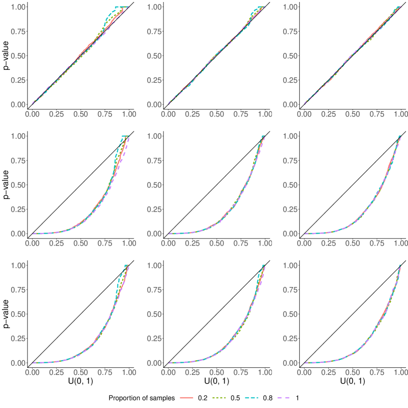
Figure 8: QQ plots of p๐‘p-values obtained using the likelihood ratio for three scenarios, using binary segmentation to estimate changepoints. Each line corresponds to the proportion of samples that were used to fit the Gaussian process.

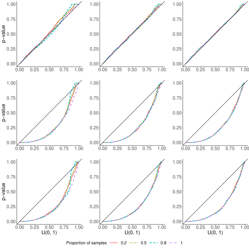
Figures 8 and 9 show QQ plots of estimated p๐‘p-values we obtain on simulated data for three different scenarios: (1) no change; (2) three changes at fixed equidistant locations, ฯ„=T4,T2,3โ€‹T4๐œ๐‘‡4๐‘‡23๐‘‡4\tau=\frac{T}{4},\frac{T}{2},\frac{3T}{4}; (3) three changes at random locations, sampled uniformly from {h,โ€ฆ,Tโˆ’h}โ„Žโ€ฆ๐‘‡โ„Ž\{h,\ldots,T-h\} and constrained to be at least hโ„Žh apart. In each case we set T=200๐‘‡200T=200 and h=20โ„Ž20h=20. For the cases with three changes, the variances on each segment were (1,4,1,0.25)1410.25(1,4,1,0.25). For each simulated data set, we estimated changepoints using binary segmentation (Figure 8) or PELT (Figure 9) and calculated an estimate of the p๐‘p-value corresponding to the first detected changepoint using a Gaussian process (as outlined in Section 3.2.2), and using a Gaussian process followed by importance sampling from the posterior distribution, for N=50,100,200๐‘50100200N=50,100,200.

Under H0subscript๐ป0H_{0}, the p๐‘p-values obtained using just a Gaussian process (i.e. the proportion of GP samples is 1) lie along the straight line implying they follow the distribution Uโ€‹(0,1)๐‘ˆ01U(0,1), whilst if we use a GP followed by importance sampling the p๐‘p-values are slightly conservative for small N๐‘N, although still close to uniform. Similarly, when we sample data with changepoints, for small N๐‘N we get slightly greater power if we just use a GP. For N=200๐‘200N=200 there seems to be very little difference between these methods. Overall, it appears that using just a Gaussian process generally gives at least as good results as using a Gaussian process followed by importance sampling.
Refer to caption

N=50๐‘50N=50N=100๐‘100N=100N=200๐‘200N=200

Figure 9: QQ plots of p๐‘p-values obtained using the likelihood ratio for three scenarios, using PELT to estimate changepoints. Each line corresponds to the proportion of samples that were used to fit the Gaussian process: where this is less than 1, the remaining samples were drawn from the posterior of the Gaussian process.

How do we know when we have enough samples? We see that N=50๐‘50N=50 seems to be sufficient in the above cases, as the estimated p๐‘p-values follow a uniform distribution under H0subscript๐ป0H_{0}, and under H1subscript๐ป1H_{1} increasing N๐‘N from 50 to 200 does not seem to lead to increased power. It is possible that we would need more samples if the number of data points T๐‘‡T or the number of changes was larger.

5.3 Increasing power

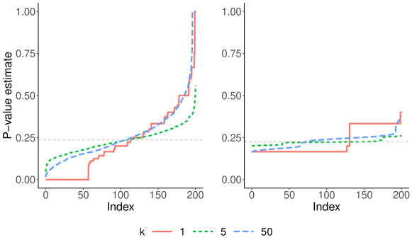
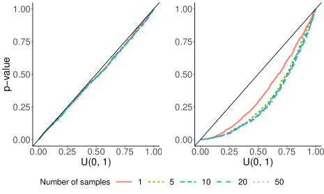
Figure 10 shows p๐‘p-values we obtained where we estimated a single changepoint using the CUSUM statistic and used the method described in Section 4.3 to calculate p๐‘p-values. We can see that under H0subscript๐ป0H_{0} (left) we obtain valid p๐‘p-values for any value of the number of samples NWsubscript๐‘๐‘ŠN_{W}. When we sample from a model with a single change at T2๐‘‡2\frac{T}{2} (right), increasing NWsubscript๐‘๐‘ŠN_{W} from 1 to 5 gives greater power against H0subscript๐ป0H_{0}, although increasing it beyond this does not seem to make much difference.
Refer to caption

H0subscript๐ป0H_{0}H1subscript๐ป1H_{1}

Figure 10: QQ plots of p๐‘p-values obtained when estimating a single changepoint using the CUSUM statistic, and calculating p๐‘p-values using the method of 4.3.

Figure 11 shows similar plots where we simulate from a model with a change at T2๐‘‡2\frac{T}{2}, and use the likelihood ratio to estimate changepoints, and a Gaussian process with Nฯ•subscript๐‘italic-ฯ•N_{\phi} samples to estimate p๐‘p-values. We see a similar pattern, where increasing the number of W๐‘ŠW samples initially leads to greater power.
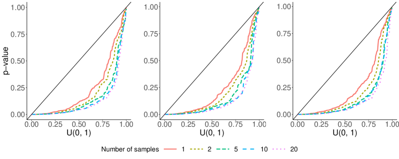
Refer to caption

Nฯ•=50subscript๐‘italic-ฯ•50N_{\phi}=50Nฯ•=100subscript๐‘italic-ฯ•100N_{\phi}=100Nฯ•=200subscript๐‘italic-ฯ•200N_{\phi}=200

Figure 11: P๐‘ƒP-values obtained sampling under H1subscript๐ป1H_{1}, and estimating a single changepoint using a Gaussian process, using the method of 4.3. Nฯ•subscript๐‘italic-ฯ•N_{\phi} is the number of ฯ•italic-ฯ•\phi samples for the Gaussian process.

6 Application to financial data

Refer to caption
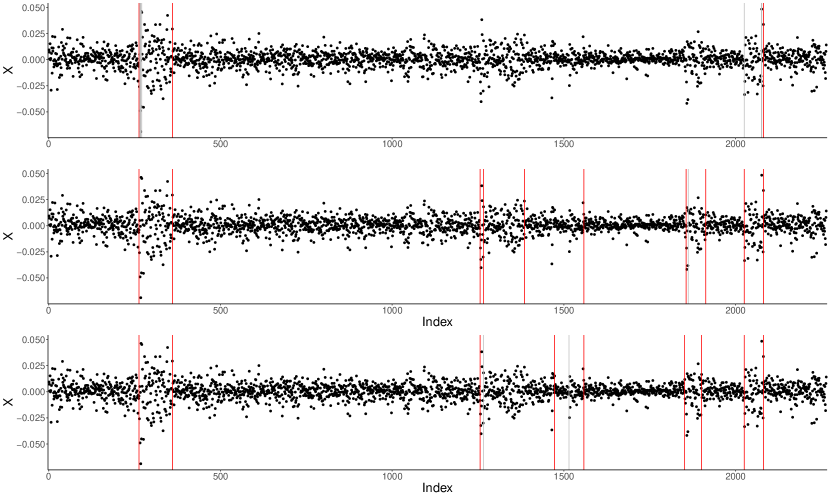
Figure 12: Application of our method to financial log returns data. Changepoints are estimated using (i) CUSUM statistic with binary segmentation (top); (ii) likelihood ratio statistic with binary segmentation (middle); (iii) likelihood ratio statistic with PELT (bottom). In each case we estimated 11 changepoints. Vertical lines indicate changepoints: those with a p๐‘p-value smaller than 0.05 (after controlling for multiple testing using the Holm-Bonferroni method) are shown in red, and those with a p๐‘p-value larger than 0.05 in grey.

To investigate how well our method works in a real-world setting, we applied our method to finanical data (Figure 12). The data is log returns from S&P500 stock market data for 2264 days from July 2010 to October 2019111The data was downloaded from https://www.kaggle.com/datasets/mathisjander/s-and-p500-volatility-prediction-time-series-data. We can see from Figure 12 that the data appears to have zero mean and several changes in variance. We estimated changepoints using three different methods: binary segmentation with the CUSUM statistic (top) and the likelihood ratio statistic (middle) and PELT (bottom), and calculated p๐‘p-values for each estimated changepoint. We set thresholds so that in each case we estimated 11 changepoints, and set h=50โ„Ž50h=50. For the cases where we had to estimate p๐‘p-values, we used a Gaussian process with N=100๐‘100N=100. On each plot estimated changepoints are shown by vertical lines, with red lines corresponding to estimated changepoint locations whose p๐‘p-values were smaller than 0.050.050.05 (after controlling for multiple testing using the Holm-Bonferroni method) and grey lines corresponding to p๐‘p-values which were not significant. Using the likelihood ratio statistic generally seems to give better results than CUSUM, where there are more instances of multiple changepoints being estimated close together. However, these spurious changepoints generally have non-significant p๐‘p-values associated with them, showing that our method for post-selection inference is effective at distinguishing true from false changepoint estimates.

7 Discussion

In this paper we have proposed a test for the piecewise constant change in variance model. We have developed methods for post-selection inference, which allow us to quantify uncertainty by computing p๐‘p-values for estimated changes, and we have shown that our methods work on simulated and real data.

We have worked on the assumption that the data is i.i.d. Gaussian except for abrupt changes in variance. In practice, less restrictive models may be more appropriate in many cases, for example allowing the mean to change as well as the variance, or allowing autocorrelation between data points. Further work in this area could include extending or adapting our approach to apply to such models.

The strategies we have developed using Gaussian processes and importance sampling may be useful for other similar situations where we conduct post-selection inference but cannot characterise the selection event explicitly.

Acknowledgement

This work is supported by EPSRC grant number EP/V053590/1.

References

  • \bibcommenthead
  • Anastasiou etย al. [2022] Anastasiou, A., Cribben, I., Fryzlewicz, P.: Cross-covariate isolate detect: A new change-point method for estimating dynamic functional connectivity. Medical Image Analysis 75, 102252 (2022)
  • Amiri etย al. [2015] Amiri, A., Niaki, S.T.A., Moghadam, A.T.: A probabilistic artificial neural network-based procedure for variance change point estimation. Soft Computing 19, 691โ€“700 (2015)
  • Baranowski etย al. [2019] Baranowski, R., Chen, Y., Fryzlewicz, P.: Narrowest-over-threshold detection of multiple change points and change-point-like features. Journal of the Royal Statistical Society: Series B 81(3), 649โ€“672 (2019)
  • Barry and Hartigan [1993] Barry, D., Hartigan, J.A.: A Bayesian analysis for change point problems. Journal of the American Statistical Association 88(421), 309โ€“319 (1993)
  • Caron etย al. [2012] Caron, F., Doucet, A., Gottardo, R.: On-line changepoint detection and parameter estimation with application to genomic data. Statistics and Computing 22, 579โ€“595 (2012)
  • Carrington and Fearnhead [2023] Carrington, R., Fearnhead, P.: Improving power by conditioning on less in post-selection inference for changepoints. arXiv preprint arXiv:2301.05636 (2023)
  • Chen etย al. [2023] Chen, Y.T., Jewell, S.W., Witten, D.M.: Quantifying uncertainty in spikes estimated from calcium imaging data. Biostatistics 24(2), 481โ€“501 (2023)
  • Cappello and Padilla [2023] Cappello, L., Padilla, O.H.M.: Bayesian variance change point detection with credible sets. arXiv preprint arXiv:2211.14097 (2023)
  • Duy and Takeuchi [2022] Duy, V.N.L., Takeuchi, I.: More powerful conditional selective inference for generalized lasso by parametric programming. The Journal of Machine Learning Research 23(1), 13544โ€“13580 (2022)
  • Eichinger and Kirch [2018] Eichinger, B., Kirch, C.: A mosum procedure for the estimation of multiple random change points. Bernoulli 24, 526โ€“564 (2018)
  • Fearnhead [2006] Fearnhead, P.: Exact and efficient Bayesian inference for multiple changepoint problems. Statistics and Computing 16, 203โ€“213 (2006)
  • Frick etย al. [2014] Frick, K., Munk, A., Sieling, H.: Multiscale change point inference. Journal of the Royal Statistical Society: Series B 76(3), 495โ€“580 (2014)
  • Fearnhead and Rigaill [2020] Fearnhead, P., Rigaill, G.: Relating and comparing methods for detecting changes in mean. Stat 9(1), 291 (2020)
  • Fryzlewicz [2014] Fryzlewicz, P.: Wild binary segmentation for multiple change-point detection. The Annals of Statistics 42(6), 2243โ€“2281 (2014)
  • Fryzlewicz [2023] Fryzlewicz, P.: Narrowest significance pursuit: inference for multiple change-points in linear models. Journal of the American Statistical Association, 1โ€“14 (2023)
  • Fryzlewicz [2024] Fryzlewicz, P.: Robust narrowest significance pursuit: Inference for multiple change-points in the median. Journal of Business & Economic Statistics, 1โ€“14 (2024)
  • Fithian etย al. [2014] Fithian, W., Sun, D., Taylor, J.: Optimal inference after model selection. arXiv:1410.2597 (2014)
  • Hyun etย al. [2021] Hyun, S., Lin, K.Z., Gโ€™Sell, M., Tibshirani, R.J.: Post-selection inference for changepoint detection algorithms with application to copy number variation data. Biometrics 77(3), 1037โ€“1049 (2021)
  • Inclan and Tiao [1994] Inclan, C., Tiao, G.C.: Use of cumulative sums of squares for retrospective detection of changes of variance. Journal of the American Statistical Association 89(427), 913โ€“923 (1994)
  • Jewell etย al. [2022] Jewell, S., Fearnhead, P., Witten, D.: Testing for a change in mean after changepoint detection. Journal of the Royal Statistical Society: Series B 84(4), 1082โ€“1104 (2022)
  • Jiang etย al. [2023] Jiang, F., Zhao, Z., Shao, X.: Time series analysis of covid-19 infection curve: A change-point perspective. Journal of econometrics 232(1), 1โ€“17 (2023)
  • Kovรกcs etย al. [2023] Kovรกcs, S., Bรผhlmann, P., Li, H., Munk, A.: Seeded binary segmentation: a general methodology for fast and optimal changepoint detection. Biometrika 110(1), 249โ€“256 (2023)
  • Killick etย al. [2012] Killick, R., Fearnhead, P., Eckley, I.A.: Optimal detection of changepoints with a linear computational cost. Journal of the American Statistical Association 107(500), 1590โ€“1598 (2012)
  • Kuchibhotla etย al. [2022] Kuchibhotla, A.K., Kolassa, J.E., Kuffner, T.A.: Post-selection inference. Annual Review of Statistics and Its Application 9, 505โ€“527 (2022)
  • Li etย al. [2016] Li, H., Munk, A., Sieling, H.: Fdr-control in multiscale change-point segmentation. Electronic Journal of Statistics 10, 918โ€“959 (2016)
  • Muggeo and Adelfio [2011] Muggeo, V.M., Adelfio, G.: Efficient change point detection for genomic sequences of continuous measurements. Bioinformatics 27(2), 161โ€“166 (2011)
  • Mehrizi and Chenouri [2021] Mehrizi, R.V., Chenouri, S.: Valid post-detection inference for change points identified using trend filtering. arXiv preprint arXiv:2104.12022 (2021)
  • Maidstone etย al. [2017] Maidstone, R., Hocking, T., Rigaill, G., Fearnhead, P.: On optimal multiple changepoint algorithms for large data. Statistics and Computing 27, 519โ€“533 (2017)
  • Meier etย al. [2021] Meier, A., Kirch, C., Cho, H.: mosum: A package for moving sums in change point analysis. Journal of Statistical Software 97(8), 1โ€“42 (2021)
  • Nam etย al. [2012] Nam, C.F., Aston, J.A., Johansen, A.M.: Quantifying the uncertainty in change points. Journal of Time Series Analysis 33(5), 807โ€“823 (2012)
  • Reeves etย al. [2007] Reeves, J., Chen, J., Wang, X.L., Lund, R., Lu, Q.Q.: A review and comparison of changepoint detection techniques for climate data. Journal of Applied Meteorology and Climatology 46(6), 900โ€“915 (2007)
  • Shi etย al. [2022] Shi, X., Beaulieu, C., Killick, R., Lund, R.: Changepoint detection: An analysis of the central England temperature series. Journal of Climate 35(19), 2729โ€“2742 (2022)
  • Schrรถder and Fryzlewicz [2013] Schrรถder, A.L., Fryzlewicz, P.: Adaptive trend estimation in financial time series via multiscale change-point-induced basis recovery. Statistics and Its Interface 6, 449โ€“461 (2013)
  • Shi etย al. [2022] Shi, X., Gallagher, C., Lund, R., Killick, R.: A comparison of single and multiple changepoint techniques for time series data. Computational Statistics & Data Analysis 170, 107433 (2022)
  • Scott and Knott [1974] Scott, A.J., Knott, M.: A cluster analysis method for grouping means in the analysis of variance. Biometrics 30, 507โ€“512 (1974)
  • Saha etย al. [2022] Saha, A., Witten, D., Bien, J.: Inferring independent sets of Gaussian variables after thresholding correlations. arXiv:2211.01521 (2022)
  • Williams and Rasmussen [2005] Williams, C.K., Rasmussen, C.E.: Gaussian Processes for Machine Learning. MIT press, Cambridge, MA (2005)

Supplementary Material for โ€œPost-selection inference for quantifying uncertainty in changes in varianceโ€
Rachel Carrington and Paul Fearnhead

Appendix A Details for (9)

As,esubscript๐ด๐‘ ๐‘’A_{s,e} and Bs,esubscript๐ต๐‘ ๐‘’B_{s,e} from (9) are given below.

As,e={0s,eโ‰คฯ„^โˆ’h1ฯ•oโ€‹bโ€‹sโ€‹โˆ‘t=ฯ„^โˆ’h+1eXt2sโ‰คฯ„^โˆ’h<eโ‰คฯ„^1ฯ•oโ€‹bโ€‹sโ€‹โˆ‘t=ฯ„^โˆ’h+1ฯ„^Xt2โˆ’11โˆ’ฯ•oโ€‹bโ€‹sโ€‹โˆ‘t=ฯ„^+1eXt2sโ‰คฯ„^โˆ’h,ฯ„^<e<ฯ„^+h1ฯ•oโ€‹bโ€‹sโ€‹โˆ‘t=ฯ„^โˆ’h+1ฯ„^Xt2โˆ’11โˆ’ฯ•oโ€‹bโ€‹sโ€‹โˆ‘t=ฯ„^+1ฯ„^+hXt2sโ‰คฯ„^โˆ’h,ฯ„^+h<e1ฯ•oโ€‹bโ€‹sโ€‹โˆ‘t=seXt2ฯ„^โˆ’h<s<eโ‰คฯ„^1ฯ•oโ€‹bโ€‹sโ€‹โˆ‘t=sฯ„^Xt2โˆ’11โˆ’ฯ•oโ€‹bโ€‹sโ€‹โˆ‘t=ฯ„^+1minโก{ฯ„^+h,e}Xt2ฯ„^โˆ’h<sโ‰คฯ„^<eโˆ’11โˆ’ฯ•oโ€‹bโ€‹sโ€‹โˆ‘t=sminโก{ฯ„^+h,e}Xt2ฯ„^<sโ‰คฯ„^+h,e>s0s,e>ฯ„^+hsubscript๐ด๐‘ ๐‘’cases0๐‘ ๐‘’^๐œโ„Ž1subscriptitalic-ฯ•๐‘œ๐‘๐‘ superscriptsubscript๐‘ก^๐œโ„Ž1๐‘’superscriptsubscript๐‘‹๐‘ก2๐‘ ^๐œโ„Ž๐‘’^๐œ1subscriptitalic-ฯ•๐‘œ๐‘๐‘ superscriptsubscript๐‘ก^๐œโ„Ž1^๐œsuperscriptsubscript๐‘‹๐‘ก211subscriptitalic-ฯ•๐‘œ๐‘๐‘ superscriptsubscript๐‘ก^๐œ1๐‘’superscriptsubscript๐‘‹๐‘ก2formulae-sequence๐‘ ^๐œโ„Ž^๐œ๐‘’^๐œโ„Ž1subscriptitalic-ฯ•๐‘œ๐‘๐‘ superscriptsubscript๐‘ก^๐œโ„Ž1^๐œsuperscriptsubscript๐‘‹๐‘ก211subscriptitalic-ฯ•๐‘œ๐‘๐‘ superscriptsubscript๐‘ก^๐œ1^๐œโ„Žsuperscriptsubscript๐‘‹๐‘ก2formulae-sequence๐‘ ^๐œโ„Ž^๐œโ„Ž๐‘’1subscriptitalic-ฯ•๐‘œ๐‘๐‘ superscriptsubscript๐‘ก๐‘ ๐‘’superscriptsubscript๐‘‹๐‘ก2^๐œโ„Ž๐‘ ๐‘’^๐œ1subscriptitalic-ฯ•๐‘œ๐‘๐‘ superscriptsubscript๐‘ก๐‘ ^๐œsuperscriptsubscript๐‘‹๐‘ก211subscriptitalic-ฯ•๐‘œ๐‘๐‘ superscriptsubscript๐‘ก^๐œ1^๐œโ„Ž๐‘’superscriptsubscript๐‘‹๐‘ก2^๐œโ„Ž๐‘ ^๐œ๐‘’11subscriptitalic-ฯ•๐‘œ๐‘๐‘ superscriptsubscript๐‘ก๐‘ ^๐œโ„Ž๐‘’superscriptsubscript๐‘‹๐‘ก2formulae-sequence^๐œ๐‘ ^๐œโ„Ž๐‘’๐‘ 0๐‘ ๐‘’^๐œโ„ŽA_{s,e}=\begin{cases}0&s,e\leq\hat{\tau}-h\\ \frac{1}{\phi_{obs}}\sum_{t=\hat{\tau}-h+1}^{e}X_{t}^{2}&s\leq\hat{\tau}-h<e\leq\hat{\tau}\\ \frac{1}{\phi_{obs}}\sum_{t=\hat{\tau}-h+1}^{\hat{\tau}}X_{t}^{2}-\frac{1}{1-\phi_{obs}}\sum_{t=\hat{\tau}+1}^{e}X_{t}^{2}&s\leq\hat{\tau}-h,\hat{\tau}<e<\hat{\tau}+h\\ \frac{1}{\phi_{obs}}\sum_{t=\hat{\tau}-h+1}^{\hat{\tau}}X_{t}^{2}-\frac{1}{1-\phi_{obs}}\sum_{t=\hat{\tau}+1}^{\hat{\tau}+h}X_{t}^{2}&s\leq\hat{\tau}-h,\hat{\tau}+h<e\\ \frac{1}{\phi_{obs}}\sum_{t=s}^{e}X_{t}^{2}&\hat{\tau}-h<s<e\leq\hat{\tau}\\ \frac{1}{\phi_{obs}}\sum_{t=s}^{\hat{\tau}}X_{t}^{2}-\frac{1}{1-\phi_{obs}}\sum_{t=\hat{\tau}+1}^{\min{\{\hat{\tau}+h,e\}}}X_{t}^{2}&\hat{\tau}-h<s\leq\hat{\tau}<e\\ -\frac{1}{1-\phi_{obs}}\sum_{t=s}^{\min{\{\hat{\tau}+h,e\}}}X_{t}^{2}&\hat{\tau}<s\leq\hat{\tau}+h,e>s\\ 0&s,e>\hat{\tau}+h\end{cases}
Bs,e={โˆ‘t=sminโก{e,ฯ„^โˆ’h}Xt2sโ‰คฯ„^โˆ’h,eโ‰คฯ„^โˆ‘t=sฯ„^โˆ’hXt2+11โˆ’ฯ•oโ€‹bโ€‹sโ€‹โˆ‘t=ฯ„^+1eXt2sโ‰คฯ„^โˆ’h<ฯ„^<eโ‰คฯ„^+hโˆ‘t=sฯ„^โˆ’hXt2+11โˆ’ฯ•oโ€‹bโ€‹sโ€‹โˆ‘t=ฯ„^+1ฯ„^+hXt2+โˆ‘t=ฯ„^+h+1eXt2sโ‰คฯ„^โˆ’h<ฯ„^+h<e0ฯ„^โˆ’h<s<eโ‰คฯ„^11โˆ’ฯ•oโ€‹bโ€‹sโ€‹โˆ‘t=ฯ„^+1eXt2ฯ„^โˆ’h<sโ‰คฯ„^<eโ‰คฯ„^+h11โˆ’ฯ•oโ€‹bโ€‹sโ€‹โˆ‘t=ฯ„^+1ฯ„^+hXt2+โˆ‘t=ฯ„^+h+1eXt2ฯ„^โˆ’h<sโ‰คฯ„^<ฯ„^+h<e11โˆ’ฯ•oโ€‹bโ€‹sโ€‹โˆ‘t=seXt2ฯ„^<s<eโ‰คฯ„^+h11โˆ’ฯ•oโ€‹bโ€‹sโ€‹โˆ‘t=sฯ„^+hXt2+โˆ‘t=ฯ„^+h+1eXt2ฯ„^<sโ‰คฯ„^+h<eโˆ‘t=seXt2s,e>ฯ„^+hsubscript๐ต๐‘ ๐‘’casessuperscriptsubscript๐‘ก๐‘ ๐‘’^๐œโ„Žsuperscriptsubscript๐‘‹๐‘ก2formulae-sequence๐‘ ^๐œโ„Ž๐‘’^๐œsuperscriptsubscript๐‘ก๐‘ ^๐œโ„Žsuperscriptsubscript๐‘‹๐‘ก211subscriptitalic-ฯ•๐‘œ๐‘๐‘ superscriptsubscript๐‘ก^๐œ1๐‘’superscriptsubscript๐‘‹๐‘ก2๐‘ ^๐œโ„Ž^๐œ๐‘’^๐œโ„Žsuperscriptsubscript๐‘ก๐‘ ^๐œโ„Žsuperscriptsubscript๐‘‹๐‘ก211subscriptitalic-ฯ•๐‘œ๐‘๐‘ superscriptsubscript๐‘ก^๐œ1^๐œโ„Žsuperscriptsubscript๐‘‹๐‘ก2superscriptsubscript๐‘ก^๐œโ„Ž1๐‘’superscriptsubscript๐‘‹๐‘ก2๐‘ ^๐œโ„Ž^๐œโ„Ž๐‘’0^๐œโ„Ž๐‘ ๐‘’^๐œ11subscriptitalic-ฯ•๐‘œ๐‘๐‘ superscriptsubscript๐‘ก^๐œ1๐‘’superscriptsubscript๐‘‹๐‘ก2^๐œโ„Ž๐‘ ^๐œ๐‘’^๐œโ„Ž11subscriptitalic-ฯ•๐‘œ๐‘๐‘ superscriptsubscript๐‘ก^๐œ1^๐œโ„Žsuperscriptsubscript๐‘‹๐‘ก2superscriptsubscript๐‘ก^๐œโ„Ž1๐‘’superscriptsubscript๐‘‹๐‘ก2^๐œโ„Ž๐‘ ^๐œ^๐œโ„Ž๐‘’11subscriptitalic-ฯ•๐‘œ๐‘๐‘ superscriptsubscript๐‘ก๐‘ ๐‘’superscriptsubscript๐‘‹๐‘ก2^๐œ๐‘ ๐‘’^๐œโ„Ž11subscriptitalic-ฯ•๐‘œ๐‘๐‘ superscriptsubscript๐‘ก๐‘ ^๐œโ„Žsuperscriptsubscript๐‘‹๐‘ก2superscriptsubscript๐‘ก^๐œโ„Ž1๐‘’superscriptsubscript๐‘‹๐‘ก2^๐œ๐‘ ^๐œโ„Ž๐‘’superscriptsubscript๐‘ก๐‘ ๐‘’superscriptsubscript๐‘‹๐‘ก2๐‘ ๐‘’^๐œโ„ŽB_{s,e}=\begin{cases}\sum_{t=s}^{\min{\{e,\hat{\tau}-h\}}}X_{t}^{2}&s\leq\hat{\tau}-h,e\leq\hat{\tau}\\ \sum_{t=s}^{\hat{\tau}-h}X_{t}^{2}+\frac{1}{1-\phi_{obs}}\sum_{t=\hat{\tau}+1}^{e}X_{t}^{2}&s\leq\hat{\tau}-h<\hat{\tau}<e\leq\hat{\tau}+h\\ \sum_{t=s}^{\hat{\tau}-h}X_{t}^{2}+\frac{1}{1-\phi_{obs}}\sum_{t=\hat{\tau}+1}^{\hat{\tau}+h}X_{t}^{2}+\sum_{t=\hat{\tau}+h+1}^{e}X_{t}^{2}&s\leq\hat{\tau}-h<\hat{\tau}+h<e\\ 0&\hat{\tau}-h<s<e\leq\hat{\tau}\\ \frac{1}{1-\phi_{obs}}\sum_{t=\hat{\tau}+1}^{e}X_{t}^{2}&\hat{\tau}-h<s\leq\hat{\tau}<e\leq\hat{\tau}+h\\ \frac{1}{1-\phi_{obs}}\sum_{t=\hat{\tau}+1}^{\hat{\tau}+h}X_{t}^{2}+\sum_{t=\hat{\tau}+h+1}^{e}X_{t}^{2}&\hat{\tau}-h<s\leq\hat{\tau}<\hat{\tau}+h<e\\ \frac{1}{1-\phi_{obs}}\sum_{t=s}^{e}X_{t}^{2}&\hat{\tau}<s<e\leq\hat{\tau}+h\\ \frac{1}{1-\phi_{obs}}\sum_{t=s}^{\hat{\tau}+h}X_{t}^{2}+\sum_{t=\hat{\tau}+h+1}^{e}X_{t}^{2}&\hat{\tau}<s\leq\hat{\tau}+h<e\\ \sum_{t=s}^{e}X_{t}^{2}&s,e>\hat{\tau}+h\end{cases}

Appendix B Proof of Lemma 2

We want to show that W1l,โ€ฆ,Whโˆ’1l,W1r,โ€ฆ,Whโˆ’1r,C02,ฯ•superscriptsubscript๐‘Š1๐‘™โ€ฆsuperscriptsubscript๐‘Šโ„Ž1๐‘™superscriptsubscript๐‘Š1๐‘Ÿโ€ฆsuperscriptsubscript๐‘Šโ„Ž1๐‘Ÿsuperscriptsubscript๐ถ02italic-ฯ•W_{1}^{l},\ldots,W_{h-1}^{l},W_{1}^{r},\ldots,W_{h-1}^{r},C_{0}^{2},\phi are independent. To do this we calculate the joint density of these variables and show that it can be factorized into functions of each variable.

Let gisubscript๐‘”๐‘–g_{i} (i=1,โ€ฆ,2h)i=1,\ldots,2h) denote the function such that Xฯ„^โˆ’h+i2=giโ€‹(๐‘พ,ฯ•,C02)superscriptsubscript๐‘‹^๐œโ„Ž๐‘–2subscript๐‘”๐‘–๐‘พitalic-ฯ•superscriptsubscript๐ถ02X_{\hat{\tau}-h+i}^{2}=g_{i}(\boldsymbol{W},\phi,C_{0}^{2}), and let ๐‘ฑ๐‘ฑ\boldsymbol{J} denote the Jacobian matrix of partial derivatives

๐‘ฑ=(โˆ‚Xฯ„^โˆ’h+12โˆ‚W1lโ€ฆโˆ‚Xฯ„^โˆ’h+12โˆ‚Whโˆ’1lโˆ‚Xฯ„^โˆ’h+12โˆ‚W1rโ€ฆโˆ‚Xฯ„^โˆ’h+12โˆ‚Whโˆ’1rโˆ‚Xฯ„^โˆ’h+12โˆ‚ฯ•โˆ‚Xฯ„^โˆ’h+12โˆ‚C02โ‹ฎโ‹ฎโˆ‚Xฯ„^+h2โˆ‚W1lโ€ฆโˆ‚Xฯ„^+h2โˆ‚Whโˆ’1lโˆ‚Xฯ„^+h2โˆ‚W1rโ€ฆโˆ‚Xฯ„^+h2โˆ‚Whโˆ’1rโˆ‚Xฯ„^+h2โˆ‚ฯ•โˆ‚Xฯ„^+h2โˆ‚C02).๐‘ฑsuperscriptsubscript๐‘‹^๐œโ„Ž12superscriptsubscript๐‘Š1๐‘™โ€ฆsuperscriptsubscript๐‘‹^๐œโ„Ž12superscriptsubscript๐‘Šโ„Ž1๐‘™superscriptsubscript๐‘‹^๐œโ„Ž12superscriptsubscript๐‘Š1๐‘Ÿโ€ฆsuperscriptsubscript๐‘‹^๐œโ„Ž12superscriptsubscript๐‘Šโ„Ž1๐‘Ÿsuperscriptsubscript๐‘‹^๐œโ„Ž12italic-ฯ•superscriptsubscript๐‘‹^๐œโ„Ž12superscriptsubscript๐ถ02โ‹ฎmissing-subexpressionmissing-subexpressionmissing-subexpressionmissing-subexpressionmissing-subexpressionmissing-subexpressionโ‹ฎsuperscriptsubscript๐‘‹^๐œโ„Ž2superscriptsubscript๐‘Š1๐‘™โ€ฆsuperscriptsubscript๐‘‹^๐œโ„Ž2superscriptsubscript๐‘Šโ„Ž1๐‘™superscriptsubscript๐‘‹^๐œโ„Ž2superscriptsubscript๐‘Š1๐‘Ÿโ€ฆsuperscriptsubscript๐‘‹^๐œโ„Ž2superscriptsubscript๐‘Šโ„Ž1๐‘Ÿsuperscriptsubscript๐‘‹^๐œโ„Ž2italic-ฯ•superscriptsubscript๐‘‹^๐œโ„Ž2superscriptsubscript๐ถ02\boldsymbol{J}=\left(\begin{array}[]{cccccccc}\frac{\partial X_{\hat{\tau}-h+1}^{2}}{\partial W_{1}^{l}}&\ldots&\frac{\partial X_{\hat{\tau}-h+1}^{2}}{\partial W_{h-1}^{l}}&\frac{\partial X_{\hat{\tau}-h+1}^{2}}{\partial W_{1}^{r}}&\ldots&\frac{\partial{X}_{\hat{\tau}-h+1}^{2}}{\partial W_{h-1}^{r}}&\frac{\partial X_{\hat{\tau}-h+1}^{2}}{\partial\phi}&\frac{\partial X_{\hat{\tau}-h+1}^{2}}{\partial C_{0}^{2}}\\ \vdots&&&&&&&\vdots\\ \frac{\partial X_{\hat{\tau}+h}^{2}}{\partial W_{1}^{l}}&\ldots&\frac{\partial X_{\hat{\tau}+h}^{2}}{\partial W_{h-1}^{l}}&\frac{\partial X_{\hat{\tau}+h}^{2}}{\partial W_{1}^{r}}&\ldots&\frac{\partial X_{\hat{\tau}+h}^{2}}{\partial W_{h-1}^{r}}&\frac{\partial X_{\hat{\tau}+h}^{2}}{\partial\phi}&\frac{\partial X_{\hat{\tau}+h}^{2}}{\partial C_{0}^{2}}\end{array}\right).

Then the density function of (๐‘พ,ฯ•,C02)๐‘พitalic-ฯ•superscriptsubscript๐ถ02(\boldsymbol{W},\phi,C_{0}^{2}) is given by

fโ€‹(๐‘พ,ฯ•,C02)=โˆi=12โ€‹hfXฯ„^โˆ’h+i2โ€‹(giโˆ’1โ€‹(๐‘พ,ฯ•,C02))โ€‹|๐‘ฑ|.๐‘“๐‘พitalic-ฯ•superscriptsubscript๐ถ02superscriptsubscriptproduct๐‘–12โ„Žsubscript๐‘“superscriptsubscript๐‘‹^๐œโ„Ž๐‘–2superscriptsubscript๐‘”๐‘–1๐‘พitalic-ฯ•superscriptsubscript๐ถ02๐‘ฑf(\boldsymbol{W},\phi,C_{0}^{2})=\prod_{i=1}^{2h}f_{X_{\hat{\tau}-h+i}^{2}}(g_{i}^{-1}(\boldsymbol{W},\phi,C_{0}^{2}))|\boldsymbol{J}|.

By (4) we have

Xฯ„^โˆ’h+i2={(1โˆ’Wiโˆ’1l)โ€‹โˆk=ihโˆ’1Wklโ€‹C02โ€‹ฯ•i=1,โ€ฆ,hโˆ’1(1โˆ’Wiโˆ’1l)โ€‹C02โ€‹ฯ•i=hXฯ„^+i2={(1โˆ’Wiโˆ’1r)โ€‹โˆk=ihโˆ’1Wkrโ€‹C02โ€‹(1โˆ’ฯ•)i=1,โ€ฆ,hโˆ’1(1โˆ’Wiโˆ’1r)โ€‹C02โ€‹(1โˆ’ฯ•)i=h.superscriptsubscript๐‘‹^๐œโ„Ž๐‘–2cases1superscriptsubscript๐‘Š๐‘–1๐‘™superscriptsubscriptproduct๐‘˜๐‘–โ„Ž1superscriptsubscript๐‘Š๐‘˜๐‘™superscriptsubscript๐ถ02italic-ฯ•๐‘–1โ€ฆโ„Ž11superscriptsubscript๐‘Š๐‘–1๐‘™superscriptsubscript๐ถ02italic-ฯ•๐‘–โ„Žsuperscriptsubscript๐‘‹^๐œ๐‘–2cases1superscriptsubscript๐‘Š๐‘–1๐‘Ÿsuperscriptsubscriptproduct๐‘˜๐‘–โ„Ž1superscriptsubscript๐‘Š๐‘˜๐‘Ÿsuperscriptsubscript๐ถ021italic-ฯ•๐‘–1โ€ฆโ„Ž11superscriptsubscript๐‘Š๐‘–1๐‘Ÿsuperscriptsubscript๐ถ021italic-ฯ•๐‘–โ„Ž\begin{split}X_{\hat{\tau}-h+i}^{2}&=\begin{cases}(1-W_{i-1}^{l})\prod_{k=i}^{h-1}W_{k}^{l}C_{0}^{2}\phi&i=1,\ldots,h-1\\ (1-W_{i-1}^{l})C_{0}^{2}\phi&i=h\end{cases}\\ X_{\hat{\tau}+i}^{2}&=\begin{cases}(1-W_{i-1}^{r})\prod_{k=i}^{h-1}W_{k}^{r}C_{0}^{2}(1-\phi)&i=1,\ldots,h-1\\ (1-W_{i-1}^{r})C_{0}^{2}(1-\phi)&i=h.\end{cases}\end{split}

Each Xt2โˆผGโ€‹aโ€‹mโ€‹mโ€‹aโ€‹(12,2โ€‹ฯƒ2)similar-tosuperscriptsubscript๐‘‹๐‘ก2๐บ๐‘Ž๐‘š๐‘š๐‘Ž122superscript๐œŽ2X_{t}^{2}\sim Gamma\left(\frac{1}{2},2\sigma^{2}\right), so fXtโ€‹(x)=(2โ€‹ฯƒ2)1/2ฮ“โ€‹(12)โ€‹xโˆ’1/2โ€‹eโˆ’2โ€‹ฯƒ2โ€‹xsubscript๐‘“subscript๐‘‹๐‘ก๐‘ฅsuperscript2superscript๐œŽ212ฮ“12superscript๐‘ฅ12superscript๐‘’2superscript๐œŽ2๐‘ฅf_{X_{t}}(x)=\frac{(2\sigma^{2})^{1/2}}{\Gamma(\frac{1}{2})}x^{-1/2}e^{-2\sigma^{2}x}.

We get

โˆi=12โ€‹hfXโ€‹(giโˆ’1โ€‹(๐‘พ,ฯ•,C02))=(2โ€‹ฯƒ2)hฮ“โ€‹(12)2โ€‹hโ€‹(โˆi=12โ€‹hXฯ„^โˆ’h+i2)โˆ’1/2โ€‹eโˆ’2โ€‹ฯƒ2โ€‹โˆ‘i=12โ€‹hXฯ„^โˆ’h+i2=(2โ€‹ฯƒ2)hฮ“โ€‹(12)2โ€‹hโ€‹โˆi=1hโˆ’1(1โˆ’Wil)โˆ’1/2โ€‹โˆi=1hโˆ’1(Wil)โˆ’i/2โ€‹โˆi=1hโˆ’1(1โˆ’Wir)โˆ’1/2โ€‹โˆi=1hโˆ’1(Wir)โˆ’i/2โ€‹eโˆ’2โ€‹ฯƒ2โ€‹C02superscriptsubscriptproduct๐‘–12โ„Žsubscript๐‘“๐‘‹superscriptsubscript๐‘”๐‘–1๐‘พitalic-ฯ•superscriptsubscript๐ถ02superscript2superscript๐œŽ2โ„Žฮ“superscript122โ„Žsuperscriptsuperscriptsubscriptproduct๐‘–12โ„Žsuperscriptsubscript๐‘‹^๐œโ„Ž๐‘–212superscript๐‘’2superscript๐œŽ2superscriptsubscript๐‘–12โ„Žsuperscriptsubscript๐‘‹^๐œโ„Ž๐‘–2superscript2superscript๐œŽ2โ„Žฮ“superscript122โ„Žsuperscriptsubscriptproduct๐‘–1โ„Ž1superscript1superscriptsubscript๐‘Š๐‘–๐‘™12superscriptsubscriptproduct๐‘–1โ„Ž1superscriptsuperscriptsubscript๐‘Š๐‘–๐‘™๐‘–2superscriptsubscriptproduct๐‘–1โ„Ž1superscript1superscriptsubscript๐‘Š๐‘–๐‘Ÿ12superscriptsubscriptproduct๐‘–1โ„Ž1superscriptsuperscriptsubscript๐‘Š๐‘–๐‘Ÿ๐‘–2superscript๐‘’2superscript๐œŽ2superscriptsubscript๐ถ02\begin{split}\prod_{i=1}^{2h}f_{X}(g_{i}^{-1}(\boldsymbol{W},\phi,C_{0}^{2}))&=\frac{\left(2\sigma^{2}\right)^{h}}{\Gamma\left(\frac{1}{2}\right)^{2h}}\left(\prod_{i=1}^{2h}X_{\hat{\tau}-h+i}^{2}\right)^{-1/2}e^{-2\sigma^{2}\sum_{i=1}^{2h}X_{\hat{\tau}-h+i}^{2}}\\ &=\frac{\left(2\sigma^{2}\right)^{h}}{\Gamma\left(\frac{1}{2}\right)^{2h}}\prod_{i=1}^{h-1}\left(1-W_{i}^{l}\right)^{-1/2}\prod_{i=1}^{h-1}\left(W_{i}^{l}\right)^{-i/2}\prod_{i=1}^{h-1}\left(1-W_{i}^{r}\right)^{-1/2}\prod_{i=1}^{h-1}\left(W_{i}^{r}\right)^{-i/2}e^{-2\sigma^{2}C_{0}^{2}}\end{split}

To calculate the determinant of ๐‘ฑ๐‘ฑ\boldsymbol{J}, note that using elementary row operations, we can show that |๐‘ฑ|๐‘ฑ|\boldsymbol{J}| is equal to the determinant of the matrix

โˆ‚Xฯ„^โˆ’h+12โˆ‚W1lโ€ฆโˆ‚Xฯ„^โˆ’h+12โˆ‚Whโˆ’1lโˆ‚Xฯ„^โˆ’h+12โˆ‚W1rโ€ฆโˆ‚Xฯ„^โˆ’h+12โˆ‚Whโˆ’1rโˆ‚Xฯ„^โˆ’h+12โˆ‚ฯ•โˆ‚Xฯ„^โˆ’h+12โˆ‚C02โˆ‘i=12โˆ‚Xฯ„^โˆ’h+i2โˆ‚W1lโ€ฆโˆ‘i=12โˆ‚Xฯ„^โˆ’h+i2โˆ‚Whโˆ’1lโˆ‘i=12โˆ‚Xฯ„^โˆ’h+i2โˆ‚W1rโ€ฆโˆ‘i=12โˆ‚Xฯ„^โˆ’h+i2โˆ‚Whโˆ’1rโˆ‘i=12โˆ‚Xฯ„^โˆ’h+i2โˆ‚ฯ•โˆ‘i=12โˆ‚Xฯ„^โˆ’h+i2โˆ‚C02โ‹ฎโ‹ฎโ‹ฎโ‹ฎโ‹ฎโ‹ฎโˆ‘i=1hโˆ’1โˆ‚Xฯ„^โˆ’h+i2โˆ‚W1lโ€ฆโˆ‘i=1hโˆ’1โˆ‚Xฯ„^โˆ’h+i2โˆ‚Whโˆ’1lโˆ‘i=1hโˆ’1โˆ‚Xฯ„^โˆ’h+i2โˆ‚W1rโ€ฆโˆ‘i=1hโˆ’1โˆ‚Xฯ„^โˆ’h+i2โˆ‚Whโˆ’1rโˆ‘i=1hโˆ’1โˆ‚Xฯ„^โˆ’h+i2โˆ‚ฯ•โˆ‘i=1hโˆ’1โˆ‚Xฯ„^โˆ’h+i2โˆ‚C02โˆ‚Xฯ„^+12โˆ‚W1lโ€ฆโˆ‚Xฯ„^+12โˆ‚Whโˆ’1lโˆ‚Xฯ„^+12โˆ‚W1rโ€ฆโˆ‚Xฯ„^+12โˆ‚Whโˆ’1rโˆ‚Xฯ„^+12โˆ‚ฯ•โˆ‚Xฯ„^+12โˆ‚C02โˆ‘i=12โˆ‚Xฯ„^+i2โˆ‚W1lโ€ฆโˆ‘i=12โˆ‚Xฯ„^+i2โˆ‚Whโˆ’1lโˆ‘i=12โˆ‚Xฯ„^+i2โˆ‚W1rโ€ฆโˆ‘i=12โˆ‚Xฯ„^+i2โˆ‚Whโˆ’1rโˆ‘i=12โˆ‚Xฯ„^+i2โˆ‚ฯ•โˆ‘i=12โˆ‚Xฯ„^+i2โˆ‚C02โ‹ฎโ‹ฎโ‹ฎโ‹ฎโ‹ฎโ‹ฎโˆ‘i=1hโˆ’1โˆ‚Xฯ„^+i2โˆ‚W1lโ€ฆโˆ‘i=1hโˆ’1โˆ‚Xฯ„^+i2โˆ‚Whโˆ’1lโˆ‘i=1hโˆ’1โˆ‚Xฯ„^+i2โˆ‚W1rโ€ฆโˆ‘i=1hโˆ’1โˆ‚Xฯ„^+i2โˆ‚Whโˆ’1rโˆ‘i=1hโˆ’1โˆ‚Xฯ„^+i2โˆ‚ฯ•โˆ‘i=1hโˆ’1โˆ‚Xฯ„^+i2โˆ‚C02โˆ‘i=1hโˆ‚Xฯ„^โˆ’h+i2โˆ‚W1lโ€ฆโˆ‘i=1hโˆ‚Xฯ„^โˆ’h+i2โˆ‚Whโˆ’1lโˆ‘i=1hโˆ‚Xฯ„^โˆ’h+i2โˆ‚W1rโ€ฆโˆ‘i=1hโˆ‚Xฯ„^โˆ’h+i2โˆ‚Whโˆ’1rโˆ‘i=1hโˆ‚Xฯ„^โˆ’h+i2โˆ‚ฯ•โˆ‘i=1hโˆ‚Xฯ„^โˆ’h+i2โˆ‚C02โˆ‘i=12โ€‹hโˆ‚Xฯ„^โˆ’h+i2โˆ‚W1lโ€ฆโˆ‘i=12โ€‹hโˆ‚Xฯ„^โˆ’h+i2โˆ‚Whโˆ’1lโˆ‘i=12โ€‹hโˆ‚Xฯ„^โˆ’h+i2โˆ‚W1rโ€ฆโˆ‘i=12โ€‹hโˆ‚Xฯ„^โˆ’h+i2โˆ‚Whโˆ’1rโˆ‘i=12โ€‹hโˆ‚Xฯ„^โˆ’h+i2โˆ‚ฯ•โˆ‘i=12โ€‹hโˆ‚Xฯ„^โˆ’h+i2โˆ‚C02.superscriptsubscript๐‘‹^๐œโ„Ž12superscriptsubscript๐‘Š1๐‘™โ€ฆsuperscriptsubscript๐‘‹^๐œโ„Ž12superscriptsubscript๐‘Šโ„Ž1๐‘™superscriptsubscript๐‘‹^๐œโ„Ž12superscriptsubscript๐‘Š1๐‘Ÿโ€ฆsuperscriptsubscript๐‘‹^๐œโ„Ž12superscriptsubscript๐‘Šโ„Ž1๐‘Ÿsuperscriptsubscript๐‘‹^๐œโ„Ž12italic-ฯ•superscriptsubscript๐‘‹^๐œโ„Ž12superscriptsubscript๐ถ02superscriptsubscript๐‘–12superscriptsubscript๐‘‹^๐œโ„Ž๐‘–2superscriptsubscript๐‘Š1๐‘™โ€ฆsuperscriptsubscript๐‘–12superscriptsubscript๐‘‹^๐œโ„Ž๐‘–2superscriptsubscript๐‘Šโ„Ž1๐‘™superscriptsubscript๐‘–12superscriptsubscript๐‘‹^๐œโ„Ž๐‘–2superscriptsubscript๐‘Š1๐‘Ÿโ€ฆsuperscriptsubscript๐‘–12superscriptsubscript๐‘‹^๐œโ„Ž๐‘–2superscriptsubscript๐‘Šโ„Ž1๐‘Ÿsuperscriptsubscript๐‘–12superscriptsubscript๐‘‹^๐œโ„Ž๐‘–2italic-ฯ•superscriptsubscript๐‘–12superscriptsubscript๐‘‹^๐œโ„Ž๐‘–2superscriptsubscript๐ถ02โ‹ฎmissing-subexpressionโ‹ฎโ‹ฎmissing-subexpressionโ‹ฎโ‹ฎโ‹ฎsuperscriptsubscript๐‘–1โ„Ž1superscriptsubscript๐‘‹^๐œโ„Ž๐‘–2superscriptsubscript๐‘Š1๐‘™โ€ฆsuperscriptsubscript๐‘–1โ„Ž1superscriptsubscript๐‘‹^๐œโ„Ž๐‘–2superscriptsubscript๐‘Šโ„Ž1๐‘™superscriptsubscript๐‘–1โ„Ž1superscriptsubscript๐‘‹^๐œโ„Ž๐‘–2superscriptsubscript๐‘Š1๐‘Ÿโ€ฆsuperscriptsubscript๐‘–1โ„Ž1superscriptsubscript๐‘‹^๐œโ„Ž๐‘–2superscriptsubscript๐‘Šโ„Ž1๐‘Ÿsuperscriptsubscript๐‘–1โ„Ž1superscriptsubscript๐‘‹^๐œโ„Ž๐‘–2italic-ฯ•superscriptsubscript๐‘–1โ„Ž1superscriptsubscript๐‘‹^๐œโ„Ž๐‘–2superscriptsubscript๐ถ02superscriptsubscript๐‘‹^๐œ12superscriptsubscript๐‘Š1๐‘™โ€ฆsuperscriptsubscript๐‘‹^๐œ12superscriptsubscript๐‘Šโ„Ž1๐‘™superscriptsubscript๐‘‹^๐œ12superscriptsubscript๐‘Š1๐‘Ÿโ€ฆsuperscriptsubscript๐‘‹^๐œ12superscriptsubscript๐‘Šโ„Ž1๐‘Ÿsuperscriptsubscript๐‘‹^๐œ12italic-ฯ•superscriptsubscript๐‘‹^๐œ12superscriptsubscript๐ถ02superscriptsubscript๐‘–12superscriptsubscript๐‘‹^๐œ๐‘–2superscriptsubscript๐‘Š1๐‘™โ€ฆsuperscriptsubscript๐‘–12superscriptsubscript๐‘‹^๐œ๐‘–2superscriptsubscript๐‘Šโ„Ž1๐‘™superscriptsubscript๐‘–12superscriptsubscript๐‘‹^๐œ๐‘–2superscriptsubscript๐‘Š1๐‘Ÿโ€ฆsuperscriptsubscript๐‘–12superscriptsubscript๐‘‹^๐œ๐‘–2superscriptsubscript๐‘Šโ„Ž1๐‘Ÿsuperscriptsubscript๐‘–12superscriptsubscript๐‘‹^๐œ๐‘–2italic-ฯ•superscriptsubscript๐‘–12superscriptsubscript๐‘‹^๐œ๐‘–2superscriptsubscript๐ถ02โ‹ฎmissing-subexpressionโ‹ฎโ‹ฎmissing-subexpressionโ‹ฎโ‹ฎโ‹ฎsuperscriptsubscript๐‘–1โ„Ž1superscriptsubscript๐‘‹^๐œ๐‘–2superscriptsubscript๐‘Š1๐‘™โ€ฆsuperscriptsubscript๐‘–1โ„Ž1superscriptsubscript๐‘‹^๐œ๐‘–2superscriptsubscript๐‘Šโ„Ž1๐‘™superscriptsubscript๐‘–1โ„Ž1superscriptsubscript๐‘‹^๐œ๐‘–2superscriptsubscript๐‘Š1๐‘Ÿโ€ฆsuperscriptsubscript๐‘–1โ„Ž1superscriptsubscript๐‘‹^๐œ๐‘–2superscriptsubscript๐‘Šโ„Ž1๐‘Ÿsuperscriptsubscript๐‘–1โ„Ž1superscriptsubscript๐‘‹^๐œ๐‘–2italic-ฯ•superscriptsubscript๐‘–1โ„Ž1superscriptsubscript๐‘‹^๐œ๐‘–2superscriptsubscript๐ถ02superscriptsubscript๐‘–1โ„Žsuperscriptsubscript๐‘‹^๐œโ„Ž๐‘–2superscriptsubscript๐‘Š1๐‘™โ€ฆsuperscriptsubscript๐‘–1โ„Žsuperscriptsubscript๐‘‹^๐œโ„Ž๐‘–2superscriptsubscript๐‘Šโ„Ž1๐‘™superscriptsubscript๐‘–1โ„Žsuperscriptsubscript๐‘‹^๐œโ„Ž๐‘–2superscriptsubscript๐‘Š1๐‘Ÿโ€ฆsuperscriptsubscript๐‘–1โ„Žsuperscriptsubscript๐‘‹^๐œโ„Ž๐‘–2superscriptsubscript๐‘Šโ„Ž1๐‘Ÿsuperscriptsubscript๐‘–1โ„Žsuperscriptsubscript๐‘‹^๐œโ„Ž๐‘–2italic-ฯ•superscriptsubscript๐‘–1โ„Žsuperscriptsubscript๐‘‹^๐œโ„Ž๐‘–2superscriptsubscript๐ถ02superscriptsubscript๐‘–12โ„Žsuperscriptsubscript๐‘‹^๐œโ„Ž๐‘–2superscriptsubscript๐‘Š1๐‘™โ€ฆsuperscriptsubscript๐‘–12โ„Žsuperscriptsubscript๐‘‹^๐œโ„Ž๐‘–2superscriptsubscript๐‘Šโ„Ž1๐‘™superscriptsubscript๐‘–12โ„Žsuperscriptsubscript๐‘‹^๐œโ„Ž๐‘–2superscriptsubscript๐‘Š1๐‘Ÿโ€ฆsuperscriptsubscript๐‘–12โ„Žsuperscriptsubscript๐‘‹^๐œโ„Ž๐‘–2superscriptsubscript๐‘Šโ„Ž1๐‘Ÿsuperscriptsubscript๐‘–12โ„Žsuperscriptsubscript๐‘‹^๐œโ„Ž๐‘–2italic-ฯ•superscriptsubscript๐‘–12โ„Žsuperscriptsubscript๐‘‹^๐œโ„Ž๐‘–2superscriptsubscript๐ถ02\begin{array}[]{cccccccc}\frac{\partial X_{\hat{\tau}-h+1}^{2}}{\partial W_{1}^{l}}&\ldots&\frac{\partial X_{\hat{\tau}-h+1}^{2}}{\partial W_{h-1}^{l}}&\frac{\partial X_{\hat{\tau}-h+1}^{2}}{\partial W_{1}^{r}}&\ldots&\frac{\partial X_{\hat{\tau}-h+1}^{2}}{\partial W_{h-1}^{r}}&\frac{\partial X_{\hat{\tau}-h+1}^{2}}{\partial\phi}&\frac{\partial X_{\hat{\tau}-h+1}^{2}}{\partial C_{0}^{2}}\\ \sum_{i=1}^{2}\frac{\partial X_{\hat{\tau}-h+i}^{2}}{\partial W_{1}^{l}}&\ldots&\sum_{i=1}^{2}\frac{\partial X_{\hat{\tau}-h+i}^{2}}{\partial W_{h-1}^{l}}&\sum_{i=1}^{2}\frac{\partial X_{\hat{\tau}-h+i}^{2}}{\partial W_{1}^{r}}&\ldots&\sum_{i=1}^{2}\frac{\partial X_{\hat{\tau}-h+i}^{2}}{\partial W_{h-1}^{r}}&\sum_{i=1}^{2}\frac{\partial X_{\hat{\tau}-h+i}^{2}}{\partial\phi}&\sum_{i=1}^{2}\frac{\partial X_{\hat{\tau}-h+i}^{2}}{\partial C_{0}^{2}}\\ \vdots&&\vdots&\vdots&&\vdots&\vdots&\vdots\\ \sum_{i=1}^{h-1}\frac{\partial X_{\hat{\tau}-h+i}^{2}}{\partial W_{1}^{l}}&\ldots&\sum_{i=1}^{h-1}\frac{\partial X_{\hat{\tau}-h+i}^{2}}{\partial W_{h-1}^{l}}&\sum_{i=1}^{h-1}\frac{\partial X_{\hat{\tau}-h+i}^{2}}{\partial W_{1}^{r}}&\ldots&\sum_{i=1}^{h-1}\frac{\partial X_{\hat{\tau}-h+i}^{2}}{\partial W_{h-1}^{r}}&\sum_{i=1}^{h-1}\frac{\partial X_{\hat{\tau}-h+i}^{2}}{\partial\phi}&\sum_{i=1}^{h-1}\frac{\partial X_{\hat{\tau}-h+i}^{2}}{\partial C_{0}^{2}}\\ \frac{\partial X_{\hat{\tau}+1}^{2}}{\partial W_{1}^{l}}&\ldots&\frac{\partial X_{\hat{\tau}+1}^{2}}{\partial W_{h-1}^{l}}&\frac{\partial X_{\hat{\tau}+1}^{2}}{\partial W_{1}^{r}}&\ldots&\frac{\partial X_{\hat{\tau}+1}^{2}}{\partial W_{h-1}^{r}}&\frac{\partial X_{\hat{\tau}+1}^{2}}{\partial\phi}&\frac{\partial X_{\hat{\tau}+1}^{2}}{\partial C_{0}^{2}}\\ \sum_{i=1}^{2}\frac{\partial X_{\hat{\tau}+i}^{2}}{\partial W_{1}^{l}}&\ldots&\sum_{i=1}^{2}\frac{\partial X_{\hat{\tau}+i}^{2}}{\partial W_{h-1}^{l}}&\sum_{i=1}^{2}\frac{\partial X_{\hat{\tau}+i}^{2}}{\partial W_{1}^{r}}&\ldots&\sum_{i=1}^{2}\frac{\partial X_{\hat{\tau}+i}^{2}}{\partial W_{h-1}^{r}}&\sum_{i=1}^{2}\frac{\partial X_{\hat{\tau}+i}^{2}}{\partial\phi}&\sum_{i=1}^{2}\frac{\partial X_{\hat{\tau}+i}^{2}}{\partial C_{0}^{2}}\\ \vdots&&\vdots&\vdots&&\vdots&\vdots&\vdots\\ \sum_{i=1}^{h-1}\frac{\partial X_{\hat{\tau}+i}^{2}}{\partial W_{1}^{l}}&\ldots&\sum_{i=1}^{h-1}\frac{\partial X_{\hat{\tau}+i}^{2}}{\partial W_{h-1}^{l}}&\sum_{i=1}^{h-1}\frac{\partial X_{\hat{\tau}+i}^{2}}{\partial W_{1}^{r}}&\ldots&\sum_{i=1}^{h-1}\frac{\partial X_{\hat{\tau}+i}^{2}}{\partial W_{h-1}^{r}}&\sum_{i=1}^{h-1}\frac{\partial X_{\hat{\tau}+i}^{2}}{\partial\phi}&\sum_{i=1}^{h-1}\frac{\partial X_{\hat{\tau}+i}^{2}}{\partial C_{0}^{2}}\\ \sum_{i=1}^{h}\frac{\partial X_{\hat{\tau}-h+i}^{2}}{\partial W_{1}^{l}}&\ldots&\sum_{i=1}^{h}\frac{\partial X_{\hat{\tau}-h+i}^{2}}{\partial W_{h-1}^{l}}&\sum_{i=1}^{h}\frac{\partial X_{\hat{\tau}-h+i}^{2}}{\partial W_{1}^{r}}&\ldots&\sum_{i=1}^{h}\frac{\partial X_{\hat{\tau}-h+i}^{2}}{\partial W_{h-1}^{r}}&\sum_{i=1}^{h}\frac{\partial X_{\hat{\tau}-h+i}^{2}}{\partial\phi}&\sum_{i=1}^{h}\frac{\partial X_{\hat{\tau}-h+i}^{2}}{\partial C_{0}^{2}}\\ \sum_{i=1}^{2h}\frac{\partial X_{\hat{\tau}-h+i}^{2}}{\partial W_{1}^{l}}&\ldots&\sum_{i=1}^{2h}\frac{\partial X_{\hat{\tau}-h+i}^{2}}{\partial W_{h-1}^{l}}&\sum_{i=1}^{2h}\frac{\partial X_{\hat{\tau}-h+i}^{2}}{\partial W_{1}^{r}}&\ldots&\sum_{i=1}^{2h}\frac{\partial X_{\hat{\tau}-h+i}^{2}}{\partial W_{h-1}^{r}}&\sum_{i=1}^{2h}\frac{\partial X_{\hat{\tau}-h+i}^{2}}{\partial\phi}&\sum_{i=1}^{2h}\frac{\partial X_{\hat{\tau}-h+i}^{2}}{\partial C_{0}^{2}}\\ \end{array}.

We can show that this matrix is upper triangular, which allows us to calculate the determinant as the product of its diagonal elements. Since

โˆ‘i=1kXฯ„^โˆ’h+i2=โˆj=khโˆ’1Wjlโ€‹C02โ€‹ฯ•,superscriptsubscript๐‘–1๐‘˜superscriptsubscript๐‘‹^๐œโ„Ž๐‘–2superscriptsubscriptproduct๐‘—๐‘˜โ„Ž1superscriptsubscript๐‘Š๐‘—๐‘™superscriptsubscript๐ถ02italic-ฯ•\sum_{i=1}^{k}X_{\hat{\tau}-h+i}^{2}=\prod_{j=k}^{h-1}W_{j}^{l}C_{0}^{2}\phi,

it follows that โˆ‘i=1kโˆ‚Xฯ„^โˆ’h+i2โˆ‚Wjl=0superscriptsubscript๐‘–1๐‘˜superscriptsubscript๐‘‹^๐œโ„Ž๐‘–2superscriptsubscript๐‘Š๐‘—๐‘™0\sum_{i=1}^{k}\frac{\partial X_{\hat{\tau}-h+i}^{2}}{\partial W_{j}^{l}}=0 for j<k๐‘—๐‘˜j<k, and clearly we also have โˆ‘i=1kโˆ‚Xฯ„^โˆ’h+i2โˆ‚Wjr=0superscriptsubscript๐‘–1๐‘˜superscriptsubscript๐‘‹^๐œโ„Ž๐‘–2superscriptsubscript๐‘Š๐‘—๐‘Ÿ0\sum_{i=1}^{k}\frac{\partial X_{\hat{\tau}-h+i}^{2}}{\partial W_{j}^{r}}=0 for all j๐‘—j. Similarly, we can show that โˆ‘i=1kโˆ‚Xฯ„^+i2โˆ‚Wjr=0superscriptsubscript๐‘–1๐‘˜superscriptsubscript๐‘‹^๐œ๐‘–2superscriptsubscript๐‘Š๐‘—๐‘Ÿ0\sum_{i=1}^{k}\frac{\partial X_{\hat{\tau}+i}^{2}}{\partial W_{j}^{r}}=0 for j<k๐‘—๐‘˜j<k, and โˆ‘i=1kโˆ‚Xฯ„^+i2โˆ‚Wjl=0superscriptsubscript๐‘–1๐‘˜superscriptsubscript๐‘‹^๐œ๐‘–2superscriptsubscript๐‘Š๐‘—๐‘™0\sum_{i=1}^{k}\frac{\partial X_{\hat{\tau}+i}^{2}}{\partial W_{j}^{l}}=0 for all k๐‘˜k. In the bottom row, as โˆ‘i=12โ€‹hXฯ„^โˆ’h+i2=C02superscriptsubscript๐‘–12โ„Žsuperscriptsubscript๐‘‹^๐œโ„Ž๐‘–2superscriptsubscript๐ถ02\sum_{i=1}^{2h}X_{\hat{\tau}-h+i}^{2}=C_{0}^{2}, all the matrix entries except the last are 0.

We get

โˆ‘i=1jโˆ‚Xฯ„^โˆ’h+i2โˆ‚Wjl=ฯ•C02โˆk=j+1hโˆ’1Wklj,=1,โ€ฆ,hโˆ’1โˆ‘i=1jโˆ‚Xฯ„^+i2โˆ‚Wjr=(1โˆ’ฯ•)โ€‹C02โ€‹โˆk=j+1hโˆ’1Wkr,j=1,โ€ฆ,hโˆ’1โˆ‘i=1hโˆ‚Xฯ„^โˆ’h+i2โˆ‚ฯ•=C02โˆ‘i=12โ€‹hโˆ‚Xฯ„^โˆ’h+i2โˆ‚C02=1.\begin{split}\sum_{i=1}^{j}\frac{\partial X_{\hat{\tau}-h+i}^{2}}{\partial W_{j}^{l}}&=\phi C_{0}^{2}\prod_{k=j+1}^{h-1}W_{k}^{l}~{}~{}~{}j,=1,\ldots,h-1\\ \sum_{i=1}^{j}\frac{\partial X_{\hat{\tau}+i}^{2}}{\partial W_{j}^{r}}&=(1-\phi)C_{0}^{2}\prod_{k=j+1}^{h-1}W_{k}^{r},~{}~{}~{}j=1,\ldots,h-1\\ \sum_{i=1}^{h}\frac{\partial X_{\hat{\tau}-h+i}^{2}}{\partial\phi}&=C_{0}^{2}\\ \sum_{i=1}^{2h}\frac{\partial X_{\hat{\tau}-h+i}^{2}}{\partial C_{0}^{2}}&=1.\end{split}

Hence,

|๐‘ฑ|=โˆi=1hโˆ’1(Wil)iโˆ’1โ€‹โˆi=1hโˆ’1(Wir)iโˆ’1โ€‹ฯ•hโˆ’1โ€‹(1โˆ’ฯ•)hโˆ’1โ€‹(C02)2โ€‹hโˆ’1.๐‘ฑsuperscriptsubscriptproduct๐‘–1โ„Ž1superscriptsuperscriptsubscript๐‘Š๐‘–๐‘™๐‘–1superscriptsubscriptproduct๐‘–1โ„Ž1superscriptsuperscriptsubscript๐‘Š๐‘–๐‘Ÿ๐‘–1superscriptitalic-ฯ•โ„Ž1superscript1italic-ฯ•โ„Ž1superscriptsuperscriptsubscript๐ถ022โ„Ž1|\boldsymbol{J}|=\prod_{i=1}^{h-1}\left(W_{i}^{l}\right)^{i-1}\prod_{i=1}^{h-1}\left(W_{i}^{r}\right)^{i-1}\phi^{h-1}(1-\phi)^{h-1}\left(C_{0}^{2}\right)^{2h-1}.

Hence, we get

fโ€‹(๐‘พ,ฯ•,C02)=(2โ€‹ฯƒ2)hฮ“โ€‹(12)2โ€‹hโˆi=1hโˆ’1((Wil)i(1โˆ’Wil))โˆ’1/2โˆi=1hโˆ’1((Wir)i)(1โˆ’Wir))โˆ’1/2(ฯ•(1โˆ’ฯ•))โˆ’h/2C0โˆ’2โ€‹heโˆ’2โ€‹ฯƒ2โ€‹C02.\begin{split}f(\boldsymbol{W},\phi,C_{0}^{2})&=\frac{(2\sigma^{2})^{h}}{\Gamma(\frac{1}{2})^{2h}}\prod_{i=1}^{h-1}\left((W_{i}^{l})^{i}(1-W_{i}^{l})\right)^{-1/2}\prod_{i=1}^{h-1}\left((W_{i}^{r})^{i})(1-W_{i}^{r})\right)^{-1/2}\left(\phi(1-\phi)\right)^{-h/2}C_{0}^{-2h}e^{-2\sigma^{2}C_{0}^{2}}.\end{split}

This can be factorized as h0โ€‹โˆi=1hโˆ’1hiโ€‹(Wil)โ€‹โˆi=1hโˆ’1hiโ€‹(Wir)โ€‹hฯ•โ€‹(ฯ•)โ€‹hCโ€‹(C02)subscriptโ„Ž0superscriptsubscriptproduct๐‘–1โ„Ž1subscriptโ„Ž๐‘–superscriptsubscript๐‘Š๐‘–๐‘™superscriptsubscriptproduct๐‘–1โ„Ž1subscriptโ„Ž๐‘–superscriptsubscript๐‘Š๐‘–๐‘Ÿsubscriptโ„Žitalic-ฯ•italic-ฯ•subscriptโ„Ž๐ถsuperscriptsubscript๐ถ02h_{0}\prod_{i=1}^{h-1}h_{i}(W_{i}^{l})\prod_{i=1}^{h-1}h_{i}(W_{i}^{r})h_{\phi}(\phi)h_{C}(C_{0}^{2}). It is also verifiable that all these variables have domain [0,1]01[0,1] (except for C02superscriptsubscript๐ถ02C_{0}^{2} which is [0,โˆž)0[0,\infty)) regardless of the values of the others. Hence these variables are all independent.

Appendix C Additional simulations

Here we include some additional simulations to those in Section 5, where we include different changepoint algorithms and parameter values.

C.1 Detecting changes using CUSUM

Refer to caption

ฯƒ22=1superscriptsubscript๐œŽ221\sigma_{2}^{2}=1(a)ฯƒ22=0.5superscriptsubscript๐œŽ220.5\sigma_{2}^{2}=0.5(b)ฯƒ22=2superscriptsubscript๐œŽ222\sigma_{2}^{2}=2(c)ฯƒ22=4superscriptsubscript๐œŽ224\sigma_{2}^{2}=4(d)

Figure 13: QQ plots of p๐‘p-values obtained using the CUSUM method, as for Figure 6, with T=1000๐‘‡1000T=1000. Data is simulated from a model with a single change at ฯ„=T/2๐œ๐‘‡2\tau=T/2, with a pre-change variance of 1, and post-change variance ฯƒ22superscriptsubscript๐œŽ22\sigma_{2}^{2}.

Figure 6 showed QQ plots of p๐‘p-values obtained for simulated data sets, where changepoints were estimated using binary segmentation with the CUSUM statistic. Here, we present similar results for two different scenarios: in Figure 13 we simulate data with T=1000๐‘‡1000T=1000 data points (compared to T=200๐‘‡200T=200 in Figure 6) and once again estimate changepoints using binary segmentation; in Figure 14 we set T=200๐‘‡200T=200 and estimate changepoints using wild binary segmentation.

In each figure, panel (a) shows the results when data was simulated under H0subscript๐ป0H_{0}; panels (b)โ€“(d) show p๐‘p-values obtained when we simulated from a model with a single changepoint at ฯ„=T/2๐œ๐‘‡2\tau=T/2, with three different values of the post-change variance. In each case we see a similar pattern of results to Figure 6.

Refer to caption

ฯƒ22=1superscriptsubscript๐œŽ221\sigma_{2}^{2}=1(a)ฯƒ22=0.5superscriptsubscript๐œŽ220.5\sigma_{2}^{2}=0.5(b)ฯƒ22=2superscriptsubscript๐œŽ222\sigma_{2}^{2}=2(c)ฯƒ22=4superscriptsubscript๐œŽ224\sigma_{2}^{2}=4(d)

Figure 14: QQ plots of p๐‘p-values obtained using the CUSUM method, as for Figure 6. Data is simulated from a model with a single change at ฯ„=T/2๐œ๐‘‡2\tau=T/2, with a pre-change variance of 1, and post-change variance ฯƒ22superscriptsubscript๐œŽ22\sigma_{2}^{2}. Here, we use wild binary segmentation to estimate changepoints.

C.2 Sampling with and without stratification

In Section 3.2.1, we discussed using stratified sampling to estimate the p๐‘p-value. Figure 15 shows plots of the p๐‘p-values we obtained for a given simulated data set, using importance sampling with and without stratification, with 200 samples in each case. (Values of ฯ•italic-ฯ•\phi are sampled from Bโ€‹eโ€‹tโ€‹aโ€‹(h2โ€‹k,h2โ€‹k)๐ต๐‘’๐‘ก๐‘Žโ„Ž2๐‘˜โ„Ž2๐‘˜Beta(\frac{h}{2k},\frac{h}{2k}) for kโˆˆ{1,5,50}๐‘˜1550k\in\{1,5,50\}; the true distribution of ฯ•italic-ฯ•\phi is Bโ€‹eโ€‹tโ€‹aโ€‹(h2,h2)๐ต๐‘’๐‘ก๐‘Žโ„Ž2โ„Ž2Beta(\frac{h}{2},\frac{h}{2}).) We can see that although the two methods have the same mean, using stratified sampling results in a much smaller variance in the p๐‘p-value estimate.

Refer to caption
Figure 15: Each plot shows the ordered p๐‘p-value estimates obtained over 1000 runs using importance sampling without stratification (left) and with stratification (right), for a simulated data set with T=200๐‘‡200T=200, and using N=200๐‘200N=200 samples each time. The importance sampling distribution is Bโ€‹eโ€‹tโ€‹aโ€‹(h2โ€‹k,h2โ€‹k)๐ต๐‘’๐‘ก๐‘Žโ„Ž2๐‘˜โ„Ž2๐‘˜Beta(\frac{h}{2k},\frac{h}{2k}) where k=1,5,50๐‘˜1550k=1,5,50. The dashed grey line corresponds to the mean estimate. The same data set was used for all p๐‘p-value estimates.

C.3 Extra simulations for Gaussian process approach

For the Gaussian process model, we use a kernel of the form

๐‘ฒโ€‹(ฯ•1,ฯ•2)=eโˆ’12โ€‹l2โ€‹|ฯ•1โˆ’ฯ•2|,๐‘ฒsubscriptitalic-ฯ•1subscriptitalic-ฯ•2superscript๐‘’12superscript๐‘™2subscriptitalic-ฯ•1subscriptitalic-ฯ•2\boldsymbol{K}(\phi_{1},\phi_{2})=e^{-\frac{1}{2l^{2}}|\phi_{1}-\phi_{2}|}, (13)

where ฯ•1,ฯ•2โˆˆ[0,1]subscriptitalic-ฯ•1subscriptitalic-ฯ•201\phi_{1},\phi_{2}\in[0,1] are two possible values of ฯ•italic-ฯ•\phi. The value l๐‘™l is a hyperparameter, which must be chosen before we fit the model. A larger l๐‘™l will lead to a smoother function p^โ€‹(ฯ•)^๐‘italic-ฯ•\hat{p}(\phi), as it will more strongly force p^โ€‹(ฯ•1)^๐‘subscriptitalic-ฯ•1\hat{p}(\phi_{1}) and p^โ€‹(ฯ•2)^๐‘subscriptitalic-ฯ•2\hat{p}(\phi_{2}) to take the same value when ฯ•1subscriptitalic-ฯ•1\phi_{1} and ฯ•2subscriptitalic-ฯ•2\phi_{2} are close together.

In Figure 16, we investigate the effect of using six different values of l๐‘™l (lโˆˆ{0.01,0.1,1,10,100,1000}๐‘™0.010.11101001000l\in\{0.01,0.1,1,10,100,1000\}), for a simulated data set. The figure displays p^โ€‹(ฯ•)^๐‘italic-ฯ•\hat{p}(\phi), shown by a black line, with observed values pโ€‹(ฯ•)๐‘italic-ฯ•p(\phi) shown as red points. For l=1,10,100,1000๐‘™1101001000l=1,10,100,1000, the estimates we obtain of pโ€‹(ฯ•)๐‘italic-ฯ•p(\phi) are very similar, and appropriately smooth: most ฯ•italic-ฯ•\phi values have p^โ€‹(ฯ•)^๐‘italic-ฯ•\hat{p}(\phi) in {0,1}01\{0,1\} (or very close to one of these values), and we expect that ๐’ฎ๐’ฎ\mathcal{S} will consist of a small number of intervals. Using l=0.01๐‘™0.01l=0.01 or l=0.1๐‘™0.1l=0.1 gives less good results. So, it seems like a value lโ‰ฅ1๐‘™1l\geq 1 is likely to give good results. In the paper we set l=100๐‘™100l=100 for all simulations and data analyses.
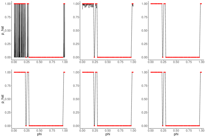
Refer to caption

l=0.01๐‘™0.01l=0.01l=0.1๐‘™0.1l=0.1l=1๐‘™1l=1l=10๐‘™10l=10l=100๐‘™100l=100l=1000๐‘™1000l=1000

Figure 16: Plots showing p^โ€‹(ฯ•)^๐‘italic-ฯ•\hat{p}(\phi) where we fit a Gaussian process with the kernel defined in (13), where l={0.01,0.1,1,10,100,1000}๐‘™0.010.11101001000l=\{0.01,0.1,1,10,100,1000\}.