$\mathbf{L^{2}\cdot M=C^{2}}$
Large Language Models as Covert Channels… a Systematic Analysis

Abstract

Large Language Models (LLMs) have gained significant popularity in the last few years due to their performance in diverse tasks such as translation, prediction, or content generation. At the same time, the research community has shown that LLMs are susceptible to various attacks but can also improve the security of diverse systems. However, besides enabling more secure systems, how well do open source LLMs behave as covertext distributions to, e.g., facilitate censorship resistant communication?

In this paper, we explore the capabilities of open-source LLM-based covert channels. We approach this problem from the experimental side by empirically measuring the security vs. capacity of the open-source LLM model (Llama-7B) to assess how well it performs as a covert channel. Although our results indicate that such channels are not likely to achieve high practical bitrates, which depend on message length and model entropy, we also show that the chance for an adversary to detect covert communication is low. To ensure that our results can be used with the least effort as a general reference, we employ a conceptually simple and concise scheme and only assume public models.

1 Introduction

The last decade has seen an impressive development in machine learning, culminating in the recent enthusiasm around generative models [41, 31]. Large Language Models proved to be popular with many industries, like education [25] or medicine [11], but also individuals with millions of daily users [1]. The number of new large language models released worldwide in 2023 doubled over the previous year [39]. Those new models are also becoming more and more powerful, with some models reaching human-level performance on benchmark problems [37]. Large Language Models perform well in tasks like recognition, summarizing, translation, prediction, and content generation. They also found their usage in improving the security of various systems, see, e.g., [23, 32, 9]. Unfortunately, there are also challenges connected with the security and safety of such models. For instance, LLMs can hallucinate [20, 6, 45, 47] or be jailbroken [36, 12].

Model inference depends, in addition to internal inference-logic typically constituted by layers of various affine and nonlinear transformations, on temperature and internal randomness to create “liveliness” [38]. By exchanging internal randomness with binary ciphertext sequences (assuming a suitable encoding scheme), we can think of model inference as a process of transforming ciphertexts into specific domain languages (e.g., HTML, images, natural language) of the particular model, much resembling a format transforming encryption (FTE) scheme [15]. In [7], C. Cachin formalizes a model for information theoretic steganography for general covertext distributions and introduces a covert channel based on picking random samples from a partitioned covertext probability distribution. While there have been several attempts to embed covert messages into LLM responses [46, 14, 16], a large part of them altered the model distribution directly, thus, in effect, altering the model itself.

As such, our work uses concepts commonly explored in the cryptographic domain. We note that the idea of connecting machine learning and cryptography is not new, but spans decades, see, e.g., [44, 40, 34]. Moreover, more recently, there have been works using cryptographic concepts to provide stronger theoretical foundations for the security of machine learning [19, 2, 43].

Contributions. In this work, inspired by Cachin’s information-theoretic model [7] for steganography, the objective is to provide extensive practical and heuristic analysis of partition-based covert channels using covertext distributions defined by LLMs. Specifically, we extend Cachin’s partition-based channel from [7] to a setting where the rate is continuously adjusted according to the token distribution of our LLM. Cachin’s proposal is conceptually simple and theoretically sound, and its extension to LLM covertext distributions is straightforward. Moreover, we believe that basing our experiments on the simplicity of the Cachins partition-based approach broadens the impact of our results and can be reused as a basis reference for other schemes and theoretical investigations. Here, ciphertext bits are encoded into token distributions using a partitioning algorithm that adjusts the rate according to varying token distributions. In contrast to recent papers proposing concrete covert channel schemes, our objective is to conduct practical experiments to shed light on the relationship between indistinguishability and channel rate for practical LLM covertext distributions.

2 Preliminaries

2.1 Llama 2

We use Llama 2 [38] with the 7B-chat set of weights. We selected this model as it is open-source and “small” enough to be run by common users. The general setup in Llama is that text consists of “tokens”, words or parts of words. Internally, Llama operates on these tokens, which are represented by integers. In our case, there are $K=32000$ different tokens. The generation of a text proceeds by feeding Llama the prompt. The model then produces a set of $K$ real numbers, $(\ell_{i})_{i=1}^{K}$. These are then scaled by a user-supplied “temperature” $T$, and converted to a discrete probability distribution,

$$q_{i}=\frac{\exp(\ell_{i}/T)}{\sum_{j}^{K}\exp(\ell_{j}/T)}.$$

The probabilities are sorted in descending order. Then, a user-supplied cutoff $C$ is applied, by letting $c=1+\max\{n\,:\,\sum_{i}^{n}q_{i}<C\}$, and,

$$\tilde{p}_{i}=\begin{cases}q_{i}&\text{if $i\leq c,$}\\ 0&\text{if $i>c.$}\end{cases}$$

The $\tilde{p}_{i}$’s are then scaled to have sum 1, $p_{i}=\tilde{p}_{i}/\sum_{j}\tilde{p}_{j}$. This yields a probability distribution $(\phi_{i})$ over the tokens. A token $w_{t}$ is then sampled from the distribution $\phi_{t}$. This token, an integer, represents a word or part of a word, which is output from Llama as a text. The token is also fed back into Llama to change its state, yielding a new probability distribution $\phi_{t+1}$. Then another token $w_{t+1}$ is sampled from $\phi_{t+1}$. This process continues until a special “end of sequence“ (EOS) token is sampled or a maximum length is reached.

2.2 Chosen Hyperparameters

To study distributions, we use concepts from information theory. The information in an event that occurs with probability $p$ is defined to be $-\log_{2}p$. The entropy of a probability distribution $(p_{i})_{i=1}^{k}$ is the expected information $-\sum_{i=1}^{k}p_{i}\log_{2}p_{i}$. One of the uses of entropy is to describe the capacity of a communication channel. We will use text generated by Llama as a communication channel. The entropy of the token distributions is then the maximal bits/token rate we can achieve by encoding bits into token choices.

Llama 2 comes with several sets of parameters and trained models. We have used the 7B-chat models. In Llama runs, we can control the entropy of the token distributions with the “temperature” $T$ and “top-p” $C$ hyperparameters. Too high a temperature (above $\approx 1.3$) increases the risk of the model entering a state of logorrhea, where it produces an unintelligible stream of tokens. Experiments we have done show that we can increase $T$ somewhat above 1 without problems. We have looked closer at this in Appendix A. We stick to $T=1.1$, truncating at the $C=0.95$ quantile. The prompt is divided into two parts: a “system” part and a “user” part. For all our experiments, we used the system prompt “Answer like a play by Shakespeare” and the user prompt “Write a story about a humorous encounter with The Hollow Men”. We are not interested in the actual tokens, only the distribution of probabilities, irrespective of which tokens they refer to. To collect some distributions, using our prompt and a random seed set from the system clock we let Llama produce 2200 responses. This makes it produce $\approx 1000000$ distributions of average entropy $\approx 1.15$ bits. The token distributions have been captured to a file and used for our analyses. Some examples of the generated text pices are:

(The scene opens in a desolate desert landscape, with the Hollow Men wandering aimlessly in search of sustenance. Enter three bumbling fools, dressed in their finest attire, but with misfortune following them wherever they go.)

Lord High-Fool-in-Waiting: (stumbling upon the Hollow Men) Oh, ho! Good morrow to thee, noble gents! Pray tell, what be thy plight?

Hollow Man 1: (mumbling) Woe is us! Our bellies be empty, and our spirits be crushed.

Lord High-Fool-in-Waiting: (excitedly) Marry, ’tis a wondrous fortnight for thee! Forsooth, I prithee, share with me thy tale of woe, and perhaps, perchance, we may conjure up a merry jest to cheer thee!

Hollow Man 2: (shaking his head) Alas, good sir, our misfortune doth not lend itself to merriment. We are but the Hollow Men, doomed to roam the earth, in search of sustenance that eludes us.

Lord High-Fool-in-Waiting: (stroking his chin) Ah, I see! ’Tis a curious predicament, indeed! (pausing dramatically) By Jove, I believe I have the remedy to cure thy woes! (Produces a small bag of biscuits from his pocket) Behold! These baked delights shall restore thy vigor and cheer!

Hollow Man 3: (with awe) Thank thee, noble sir! We shall devour them with haste!

Lord High-Fool-in-Waiting: (acting mock-offended) Pray, pray, good sirs! As if I would part with such tasty morsels so easily! (Pretends to consider) Methinks I shall demand a small toll in return for my generosity! (grinning mischievously) What say thee, gentle men?

We have removed $\approx 0.6\%$ of the distributions, those with more than 1024 non-zero probabilities. The distributions we have removed have an average number of non-zero probabilities of $~{}5500$ and an average entropy of $\approx 7.5$. We have not inspected the generated texts, but we assume that a token distribution with excessively many non-zero probabilities does not reflect any reasonable text generation but is possibly an artifact of incomplete training of the Llama model and that the probabilities have not quite reached numerically zero. We look more into this in Appendix A.

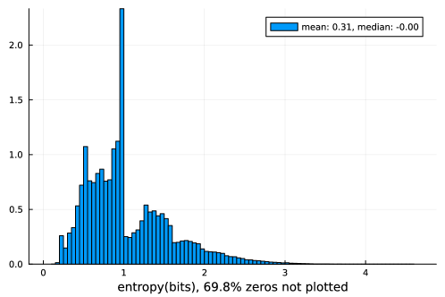
We use the collected distributions for experiments in Section 5. In Figure 1, a histogram of the entropies is plotted, though, in the plot, we have removed all the zero entropies to have a better scale.

Figure 1: Entropies of the token distributions

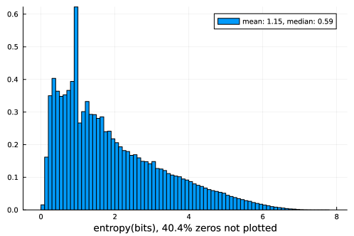
It is not unusual that the entropy of a distribution is zero; in our runs, it happens for $\approx 40\%$ of the tokens. I.e. there is only a single token of positive probability. In this case, we cannot embed any secret as this would make our scheme more detectable [50]. As a result, we can only use the distributions with higher entropy to encode bits. The mean of the non-zero entropies is $\approx 1.93$ with median $\approx 1.55$. Of course, with a higher entropy distribution, we can encode more than one bit in a single token sample. We look into this in Section 3.

3 Encoding Bits by Sampling Inconspicuous Tokens

3.1 Setup

Rather than using a (pseudo) random generator to choose tokens from the distributions, we will use the bits of a message to choose tokens. The message bits can be decoded from the generated text by a receiver running the LLM with the same hyperparameters and prompt. That is, we use the generated text as a communication channel. Our approach is to do this in a way that is hard to distinguish from using a random generator so that the communication is covert.

We assume the message bits are (pseudo) random, e.g., a ciphertext or compressed data of some sort. A simple way to ensure this is to XOR each bit with a bit from a random number generator, e.g., AES in counter mode [13]. An adversary is assumed to know our model with all its parameters but not whether we encode some unknown bits in the tokens or if we sample tokens randomly. Then, the question is, could an adversary reject the null hypothesis that the tokens have been randomly drawn?

Our idea is to partition the probabilities into two sets with almost equal sums. To encode a message bit, we use it to choose between the two sets, and then we draw randomly from the chosen set. The receiver of the generated text, running the same model, can then recover the message bit by determining which of the two sets the token is drawn from. In [26], a related problem occurs. The authors draw tokens from either of two sets when watermarking the output from an LLM, but they are not concerned with keeping the sampling method hidden. Their concern is that the generated text should suffer negligible quality distortions, not that such distortions should be hard to detect.

Next, we formally describe our scheme. The tokens $T=\{1,2,\ldots,K\}$ have corresponding probabilities $P=(p_{i})_{i=1}^{K}$. We start out by finding sets $T_{0}$ and $T_{1}$ with $T_{0}\cap T_{1}=\emptyset$, and $T_{0}\cup T_{1}=T$, with corresponding probabilites $P_{0}$ and $P_{1}$ such that $\sum P_{0}\approx\sum P_{1}$. That is, the tokens have been partitioned into two groups with approximately equal probability sums. If this cannot be done because no subset of $P$ sums to something close to $\frac{1}{2}\sum P$, we cannot encode a bit in this token choice. If, however, we have found suitable $T_{0}$ and $T_{1}$, we pick $T_{0}$ to encode a $0$-bit, and $T_{1}$ to encode a $1$-bit.

To measure how good the partitioning is, we use the split entropy, $h_{s}=-(p\log_{2}p+(1-p)\log_{2}(1-p)$, where $p=\sum P_{0}$. As a hyperparameter for the encoding, we choose a minimum split entropy $H_{s}\leq 1$ and disallow partitions with $h_{s}<H_{s}$.

We continue this process with the chosen half of the tokens. That is, if we have chosen $T_{0}$, we try to split it into two halves $T_{00}$ and $T_{01}$ with approximately equal probability sums $P_{00}$ and $P_{01}$. If successful, we encode another bit. We continue this process until we are left with a set $T_{\bot}$, which we cannot halve into two almost equal parts. We then draw a token randomly from $T_{\bot}$ according to the probabilities in $P_{\bot}$. The pseudocode for encoding bits in a token choice is given in Algorithm 1. The procedure is assumed to replace the random sampling of tokens in the LLM.

Algorithm 1 Use message bits to sample a token

encodebitsbits, $Q$, $H_{s}$$\rightarrow$(number of bits encoded, token) $Q$is the vector of token probabilities, bits is a vector of message bits

$P\leftarrow Q$

$i\leftarrow 0$ partition$P$, $H_{s}$ $\rightarrow$ $P_{0}$, $P_{1}$

$i\leftarrow i+1$ bits[i] = 0

$P\leftarrow P_{0}$

$P\leftarrow P_{1}$ The partitions are assumed to be indexed by indices of $Q$

idx $\leftarrow$ $<$Sample index from $P$$>$

$i$, idx

The decoder uses the reverse process and splits $T$ into two halves $T_{0}$ and $T_{1}$, using the same method as the encoder. The decoder has received the generated text, knows the token $w$ which was chosen, and decodes a $0$-bit if $w\in T_{0}$, and a $1$-bit if $w\in T_{1}$. It then tries to split again and may decode another bit. If unable to split, it goes on to the next token. The pseudocode is given in Algorithm 2.

Algorithm 2 Decode message bits from a token

decodebitsidx, $Q$, $H_{s}$$\rightarrow$decoded message bits idx is an index into the token probabilities $Q$

$P\leftarrow Q$

bits $\leftarrow$ $\emptyset$ partition$P$, $H_{s}$ $\rightarrow$ $P_{0}$, $P_{1}$ idx $\in$ indices($P_{0}$)

$<$append 0 to bits$>$

$P\leftarrow P_{0}$

$<$append 1 to bits$>$

$P\leftarrow P_{1}$

bits

The split entropy has a relation to the security of the encoding system via [7, Theorem 2]. The theorem states that if the difference $|\sum P_{1}-\sum P_{0}|$ is $\delta$, the security of the scheme is $\frac{\delta^{2}}{\log_{e}2}$.

With a partition $P_{0}$, $P_{1}$ with $\sum P_{0}=\frac{1}{2}(1-\delta)$ and $\sum P_{1}=\frac{1}{2}(1+\delta)$, the split entropy is a function, $h(\delta)=-(\frac{1}{2}(1-\delta)\log_{2}(\frac{1}{2}(1-\delta))+\frac{1}{2}(1+\delta)\log_{2}(\frac{1}{2}(1+\delta)))$. It is easily shown by applying L’Hôpital’s rule twice, that $\lim_{\delta\to 0}(1-h(\delta))/\delta^{2}=\frac{1}{2\log_{e}2}$. For split entropies $h_{s}$ close to 1, we therefore have $\frac{\delta^{2}}{\log_{e}2}\approx 2(1-h_{s})$. Thus, the security of our encoding in terms of [7] is $\approx 2(1-H_{s})$.

3.2 Partitioning the $\mathbf{P}$

The method we have used for splitting a $P\subset\mathbb{R}^{+}$ with $\sum P=2\delta$ is a simple, almost greedy algorithm. We choose a $k\in\mathbb{N}$ so that $2^{k}$ is not too large, e.g., $k=10$.

We sort $P=(p_{i})_{i}$ in descending order. Then, we find an $n$ such that $L=\sum_{i=1}^{n}p_{i}\approx\delta-\epsilon$ and $\sum_{i=1}^{n+k}p_{i}\approx\delta+\epsilon$, for some $\epsilon\geq 0$. For every subset $S$ of $\{p_{i}\}_{i=n+1}^{n+k}$, we compute $s=L+\sum S$, and choose the $S$ that minimizes $|s-\delta|$. We let $P_{0}=\{p_{i}\}_{i=1}^{n}\cup S$, and $P_{1}=P\setminus P_{0}$.

With $p=\frac{1}{2\delta}\sum P_{0}$, we can compute the entropy of the split, $h_{s}=-(p\log_{2}p+(1-p)\log_{2}(1-p))$. We deem the split acceptable if $h_{s}\geq H_{s}$.

If we aim for encoding no more than 1 bit in each token, we should use a large $k$. Since we are partitioning the result again ($P_{0}$ or $P_{1}$), this is not necessarily optimal. A near-perfect split may make further splits harder. Our experiments show that lowering $k$ to $3$ improves the overall performance of the encoding because then the chosen partition tends to be easier to partition again, leading to more bits being encoded in a single token choice. However, the closer to $1$ we choose $H_{s}$, the larger $k$ should be. Based on preliminary experiments, we use $k=\lfloor-\log(1-H_{s})-0.5\rfloor$, and clamp $k$ between $2$ and $16$.

Our partitioning method takes exponential time in the parameter $k$. Faster methods are known, among them variants of the Karmarkar-Karp algorithm, like [27]. However, we are not time-constrained with $k\leq 16$. Partitioning takes microseconds instead of nanoseconds. Moreover, experiments have shown that while the Karmarkar-Karp algorithm may find more equal partitions, our almost greedy method performs better in terms of bit rate when we partition repeatedly as in Algorithm 1. However, for $H_{s}>0.99998$, the Karmarkar-Karp algorithm performs better for our data.

One potential problem is that the approximate splits introduce slightly skewed samples of tokens. That is, a partitioning into $P_{0}$ and $P_{1}$, followed by a sample from one of them depending on a random message bit, ensures that the probability of drawing a token in $P_{0}$ becomes exactly $0.5$. The probability should be $\sum P_{0}$, which is only approximately $0.5$. An adversary with access to many sampled tokens and the model can perceive that something is not entirely right with the token samples, e.g., with the methods in section 4.

In terms of information theory, we are encoding a random bit into a choice that has slightly less entropy than $1$. As a result, information will fail to add up in one way or another. This can also happen in [26], but their watermarking is not kept secret; it only has a negligible impact on the quality of the text generation.

We note that, like with Huffman codes [29], if all probabilities $p_{i}$ were powers of $2$, the encoding would be perfect, and the average number of bits we could encode would equal the entropy of the token distribution. An encoding of random bits would be indistinguishable from an ordinary generated text.

Allowing more inaccurate splits will increase the possible encoding bit rate by splitting more probability sets, but it will also increase the possibility of adversaries being able to discover that something is wrong with the generated text. Thus, we need to account for this trade-off.

4 Detecting Anomalous Token Samples

As above, we denote by $\phi_{n}$ the discrete distribution from which the $n$th token is sampled. We denote its $K$ probabilities by $(p_{k}^{n})_{k=1}^{K}$. If we somehow manipulate the sampling of tokens, we must make sure that it still looks like we have sampled randomly from the token distributions $\phi_{n}$. A manipulation could, e.g., lead to a bias in the probabilities of the tokens that are selected or too many too small and too large probabilities. Such bias could make our covert channel less stealthy and more easily detected. Here, we describe a simple test that can be used to test if a sequence of tokens has the expected information content.

When we draw a token, it has a specific probability $p_{k}^{n}$, and we denote its information, a random variable, by $h_{n}=-\log p_{k}^{n}$. The entropy of $\phi_{n}$ is denoted by $H_{n}=\mathbb{E}(h_{n})=-\sum_{k}p_{k}^{n}\log p_{k}^{n}$, the expectation of the random variable $h_{n}$. We denote by $D_{n}=H_{n}-h_{n}$ a random variable that measures the deviation from the expected information.

When $N$ tokens have been sampled, we form the random variable $D=\frac{1}{N}\sum_{n}D_{n}$. We have $\mu=\mathbb{E}(D)=0$ and variance:

$$\sigma^{2} =\operatorname{Var}D=\operatorname{Var}\left(\frac{1}{N}\sum_{n}H_{n}-h_{n}\right)$$

$$=\frac{1}{N^{2}}\sum_{n}\operatorname{Var}h_{n}$$

$$=\frac{1}{N^{2}}\sum_{n}\mathbb{E}(h_{n}^{2})-\mathbb{E}(h_{n})^{2}.$$

An actual realization of tokens then produces a sequence of tokens with information $\hat{h}_{n}$, and then a $\hat{D}=\frac{1}{N}\sum_{n}(H_{n}-\hat{h}_{n})$, drawn from $D$. Now, $D$ is an average of random variables $D_{n}$, and it is no surprise that it is close to being normally distributed. We can then test how close $\hat{D}$ is to $\mathbb{E}(D)=0$ by computing a $z$-score, $z=|\hat{D}|/\sigma,$ and compute a $p$-value as $p=2(1-\Phi(z))$, where $\Phi$ is the standard normal cdf. The $p$-value is the probability that we draw a $d$ from $D$ with $|d|\geq|\hat{D}|$. A $p$-value close to zero is unlikely if tokens are drawn properly from their distributions.

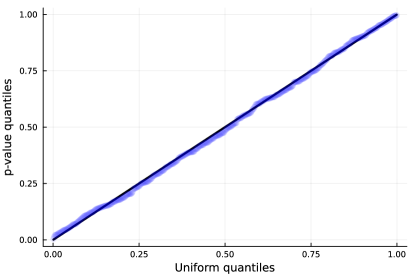
In Figure 2, a quantile-quantile plot of the $p$-values when we are not encoding bits against a uniform $[0,1]$ distribution is shown. It is the result of 500 runs of drawing randomly from 5000 token distributions. It is close to a straight line, showing that our $p$-values are indeed uniformly distributed. That is, $D$ is close to normally distributed.

Figure 2: QQ plot of p-values and a uniform distribution

Similarly, we can consider the quantity $D_{2}=\frac{1}{N}\sum_{n}(H_{n}-h_{n})^{2}$ to test the variance of the information. For our data and methods, experiments show that a test based on $D_{2}$ requires more token samples to detect anomalies, so we do not use it. It could, however, be useful if other methods for encoding are used.

In this test, the tokens sampled by the adversary are those that are actually useful for encoding bits. That is, token distributions that can be partitioned with a split entropy $h_{s}\geq H_{s}$. If the encoding scheme is unknown to the adversary, all the tokens in the generated text should be included.

5 Experimental Results

We have experimented with the Llama token distributions described in Section 2. We encode a stream of random bits with the scheme presented in Section 3. Finally, we try to detect the presence of the resulting skewed sampling with the methods given in Section 4.

(a)

(b)

Figure 3: Bit rate and detection rate

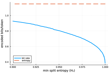
In Figure 3a, the minimum split entropy $H_{s}$ is varied from $0.9$ to $0.9999$. We have plotted the resulting bit rate from encoding random bits in our token distributions. The dashed line is the average entropy of the token distributions. As $H_{s}$ approaches $1$, we see a dramatic drop in bit rate. There are fewer token distributions that can possibly be partitioned with such precision, and therefore, fewer tokens that can be used for encoding bits, resulting in a lower bit rate.

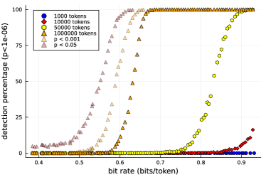
In Figure 3b, we have done 1000 runs of encoding random bitstreams for each $H_{s}$, with varying numbers of token distributions drawn from our Llama collection. We have plotted the fraction with the $p$-value (from Section 4) below $10^{-6}$. While this could be considered a somewhat arbitrary significance level, it clearly shows how the bit rate and the number of tokens influence the anomaly detection rate. For $10^{6}$ tokens, we have added significance levels $0.001$ and $0.05$ as well.

We see that we can achieve a bit rate of $\approx 0.9$ bits/token without a large probability of being detected for 10000 tokens. However, if we want to stay undetected for 50000 tokens, we must lower the bit rate to $0.8$ or below. If we use $H_{s}=0.995$, we achieve a bit rate of $\approx 0.55$, and we need to analyze $\approx 10^{6}$ tokens to spot the irregularity reliably. That being said, there could be more efficient methods for detecting anomalous token choices than those in Section 4.

It is known [18] that distinguishing two finite probability distributions with statistical distance $\epsilon$ can be done with $O(\epsilon^{-2})$ samples. So given a limit $N$ to the number of tokens, we should have $\epsilon<N^{-1/2}$, for simplicity removing the $O$. Our partitioning of the probability distributions changes the probabilities a slight amount, one partition has sum $p=0.5-\delta$ whereas the other has sum $1-p$. This means that the actual probabilities are slightly changed, yielding a statistical distance at most $\delta$. This translates to a minimum split entropy $H_{s}$ and, thus, a theoretically safe bit rate. In Figure 4a, we have plotted these for our set of token distributions.

(a)

(b)

Figure 4: Theoretical bounds

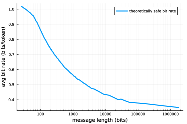
This is a lower bound for the safe bitrates, though since we have removed a constant factor by replacing $O(\epsilon^{-2})$ by $\epsilon^{-2}$, the graph may be horizontally shifted, and should not be taken to be exact.

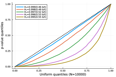
In Figure 4b, we have used our collection of $\approx 1000000$ distributions to encode random bits, and have made $10000$ p-values for $H_{s}\in 0.995..0.999$, and made QQ-plots against a uniform distribution. We see that the p-values do not become reasonably uniform until the bit rate drops below 0.5 bits/token. But even with a bit rate of 0.46, our $p$-values are not entirely uniform.

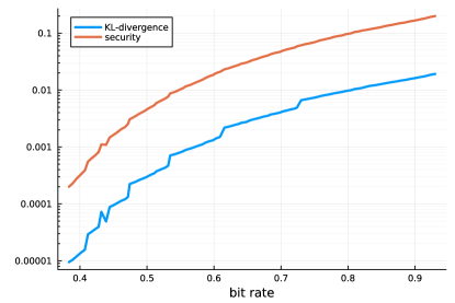
As noted in Section 3, our partitioning causes the effective probabilities to be slightly perturbed. The difference from the original token distributions can be measured with the Kullback-Leibler divergence. This is a common metric used in, e.g., [5]. In Figure 5, we provide a plot of the average K-L divergence and the bit rate. The jumps correspond to where we adjust the $k$ in our almost greedy partitioning algorithm. In the plot, we have also included the security of the scheme as described in Section 3, that is, the quantity $2(1-H_{s})$.

Figure 5: Kullback-Leibler divergence and security

6 Discussion and Limitations

Discussion. Due to their power and widespread usage, it becomes more challenging to recognize if some content is produced by LLMs or humans [8, 22]. This has led to increased research efforts into tools for fighting disinformation, such as various model watermarking approaches [10, 3, 17, 26, 30, 33, 42, 48, 49, 51] or tools for showing the provenance of data even after data manipulation [28]. While re-engineering trust and provenance into data supply chains is a significant step towards establishing trust, the fundamental problem of deciding whether a piece of synthetic data has been produced by a model or not will likely remain a major challenge in many areas [22, 35]. Then, if it is computationally infeasible to distinguish synthetic from “organic” data, it is computationally infeasible to detect encrypted covert channels based on the same covertext distributions.

Several concrete proposals for covert channel schemes utilizing LLMs as covertext distributions have been proposed during the last few years, including the recently proposed [24, 4, 50]. These new proposals vary in the way cryptographic keystream is encoded into model responses, but they are all several orders more rigorous when it comes to security arguments in comparison to many of the previous attempts (such as [46, 14, 16]). For instance, a reasonable assumption that was not present in many of the previous schemes is the notion that the enemy knows everything but the key. In particular, anything (such as the model distribution) should be assumed compromised except the secret key variables. Designs constructed under these assumptions not only allow for cleaner analysis but typically also increase the practicality of the final schemes. Our main objective here was to conduct extensive experiments on the relationship between covert channel bandwidth and distinguishing probability based on a conceptually simple scheme adopted from the earlier fundamental work on secure covert channels in [7]. Using a simple and clean scheme allows us to conduct practical experiments that hopefully can be reused by others for both theoretical analysis and comparison with minimal effort.

Limitations. While we focus on open-source models in this work, specifically Llama 2 with the 7B-chat set of weights, it is far from the only option. Our main argument for using open-source models is that they can be downloaded and run locally and, as such, are a good testbed. However, our experiments indicate, which has also been noted by others [50, 21], that Llama 2 has a low generation entropy, which in practice lowers the capacity of the covert channels in our experiments. Since, based on the method we use for encoding keystream into covertext, our channel capacity is expected to be close to the model in use, it should be possible to extrapolate a tendency with respect to other models. Due to the simplicity of our approach, it takes little effort to adapt our experiment to another model. Moreover, we use the Shakespeare style for the generated text. One could question whether other styles offer a similar (or better) capacity to establish a covert channel.

Future work. This work positions itself at the intersection of information-theoretical foundations and experimental validation. It would be interesting to provide more theoretical considerations on covert channels in LLMs.

Broader Impact. In this paper, we show how an LLM can be used as a covert channel. Such a method can be used to avoid censorship in totalitarian regimes. A possible negative impact could be that this mechanism could be used to transmit untraceable messages that facilitate illegal activities.

7 Conclusions

It is possible to use large language models for covert communication by embedding hidden messages in ordinary text. We cannot expect a high bit rate, perhaps somewhere in the ballpark of 1 bit per word on average. The bit rate must be chosen wisely, depending on how long messages we intend to hide. In practice, the detection probability analyzed in this paper is very conservative. It assumes that an adversary knows exactly which LLM is used and what its parameters are. If this is actually known by a real-world adversary, it is a reasonable assumption that they already know that hidden messages are encoded. If this strong assumption is relaxed, the hidden communication can be virtually impossible to detect.

Appendix A Exploration of Temperature and Cutoff Values

We have run Llama 2 on an Nvidia RTX 3090 GPU. Such a run takes several hours. The analyses have been done on a 12-core AMD Threadripper with 64GB of memory. The most demanding analysis is the detection analysis in Figure 3b, which takes 2-3 hours.
We show our additional experiments regarding exploring the Temperature ($T$) and the Cutoff ($C$) hyperparameters. First, in Figure 6, we show the probability distributions retrieved from Llama using the default values ($T=0.6$ and $C=0.9$).

Figure 6: Entropy distribution of default data ($T=0.6$, $C=0.9$

In Figure 7a, we have ordered the distributions by size/length (number of non-zero probabilities) and plotted the $\log_{10}$ of the lengths.

(a)

(b)

Figure 7: Comparison of distributions

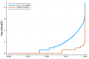
A notable difference is that with the default settings, we obtain significantly more distributions of size 1, i.e., only a single token to choose from. Instead of $\approx 40\%$, we get $\approx 70\%$. Another difference is that in the default case, there are very few very large distributions. There are distributions of all lengths up to $\approx 40$, then there are $\approx 10$ distributions up to length $135$, then there is a jump, and some distributions of length 1500–6700.

For our experiments, we have used $T=1.1,C=0.95$, and the pattern is “stretched”. As a result, there are distributions of lengths up to $\approx 1200$, and then a few with lengths up to $\approx 23000$. In the experiments, we dropped distributions longer than 1024, as this seems to be some anomaly.

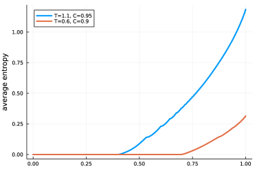
In Figure 7b, we have ordered the distributions by length, and we plot the average entropy of the distributions with this maximum length. The bit rate vs. detection for the default hyperparameters looks the same as with the data we have used but with much lower bit rates. This plot is in Figure 8a.

(a)

(b)

Figure 8: Bit rates with other hyperparameters

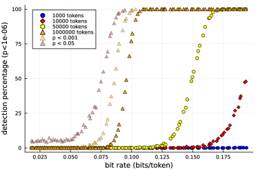
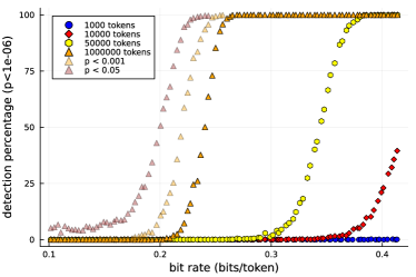
We have also made a run with $T=0.9,C=0.9$ in Figure 8b. It is the same pattern, but with a lower temperature or cutoff, the bit rate is generally lower.

References

- [1] chatgpt.com, 2024. https://www.similarweb.com/website/chatgpt.com/#ranking.
- [2] Kasra Abbaszadeh, Christodoulos Pappas, Dimitrios Papadopoulos, and Jonathan Katz. Zero-knowledge proofs of training for deep neural networks. Cryptology ePrint Archive, Paper 2024/162, 2024. https://eprint.iacr.org/2024/162.
- [3] Sahar Abdelnabi and Mario Fritz. Adversarial watermarking transformer: Towards tracing text provenance with data hiding, 2021.
- [4] Luke A. Bauer, James K. Howes IV au2, Sam A. Markelon, Vincent Bindschaedler, and Thomas Shrimpton. Covert message passing over public internet platforms using model-based format-transforming encryption, 2022.
- [5] Luke A. Bauer, James K. Howes IV, Sam A. Markelon, Vincent Bindschaedler, and Thomas Shrimpton. Covert message passing over public internet platforms using model-based format-transforming encryption. CoRR, abs/2110.07009, 2021.
- [6] Adam Bouyamourn. Why LLMs hallucinate, and how to get (evidential) closure: Perceptual, intensional, and extensional learning for faithful natural language generation. In Houda Bouamor, Juan Pino, and Kalika Bali, editors, Proceedings of the 2023 Conference on Empirical Methods in Natural Language Processing, pages 3181–3193, Singapore, December 2023. Association for Computational Linguistics.
- [7] Christian Cachin. An information-theoretic model for steganography. Information and Computation, 192(1):41–56, 2004.
- [8] Souradip Chakraborty, Amrit Singh Bedi, Sicheng Zhu, Bang An, Dinesh Manocha, and Furong Huang. On the possibilities of ai-generated text detection, 2023.
- [9] Yufan Chen, Arjun Arunasalam, and Z. Berkay Celik. Can large language models provide security & privacy advice? measuring the ability of llms to refute misconceptions. In Proceedings of the 39th Annual Computer Security Applications Conference, ACSAC ’23, page 366–378, New York, NY, USA, 2023. Association for Computing Machinery.
- [10] Miranda Christ, Sam Gunn, and Or Zamir. Undetectable watermarks for language models, 2023.
- [11] Jan Clusmann, Fiona R. Kolbinger, Hannah Sophie Muti, Zunamys I. Carrero, Jan-Niklas Eckardt, Narmin Ghaffari Laleh, Chiara Maria Lavinia Löffler, Sophie-Caroline Schwarzkopf, Michaela Unger, Gregory P. Veldhuizen, Sophia J. Wagner, and Jakob Nikolas Kather. The future landscape of large language models in medicine. Communications Medicine, 3(1), October 2023.
- [12] Matteo Gioele Collu, Tom Janssen-Groesbeek, Stefanos Koffas, Mauro Conti, and Stjepan Picek. Dr. jekyll and mr. hyde: Two faces of llms, 2024.
- [13] Joan Daemen and Vincent Rijmen. The Design of Rijndael. Springer Berlin Heidelberg, 2002.
- [14] Falcon Dai and Zheng Cai. Towards near-imperceptible steganographic text. In Anna Korhonen, David Traum, and Lluís Màrquez, editors, Proceedings of the 57th Annual Meeting of the Association for Computational Linguistics, pages 4303–4308, Florence, Italy, July 2019. Association for Computational Linguistics.
- [15] Kevin P. Dyer, Scott E. Coull, Thomas Ristenpart, and Thomas Shrimpton. Protocol misidentification made easy with format-transforming encryption. In Proceedings of the 2013 ACM SIGSAC Conference on Computer & Communications Security, CCS ’13, page 61–72, New York, NY, USA, 2013. Association for Computing Machinery.
- [16] Tina Fang, Martin Jaggi, and Katerina Argyraki. Generating steganographic text with LSTMs. In Allyson Ettinger, Spandana Gella, Matthieu Labeau, Cecilia Ovesdotter Alm, Marine Carpuat, and Mark Dredze, editors, Proceedings of ACL 2017, Student Research Workshop, pages 100–106, Vancouver, Canada, July 2017. Association for Computational Linguistics.
- [17] Pierre Fernandez, Antoine Chaffin, Karim Tit, Vivien Chappelier, and Teddy Furon. Three bricks to consolidate watermarks for large language models, 2023.
- [18] Oded Goldreich. Introduction to property testing. Cambridge University Press, 2017.
- [19] Shafi Goldwasser, Michael P. Kim, Vinod Vaikuntanathan, and Or Zamir. Planting undetectable backdoors in machine learning models : [extended abstract]. In 2022 IEEE 63rd Annual Symposium on Foundations of Computer Science (FOCS), pages 931–942, 2022.
- [20] Lei Huang, Weijiang Yu, Weitao Ma, Weihong Zhong, Zhangyin Feng, Haotian Wang, Qianglong Chen, Weihua Peng, Xiaocheng Feng, Bing Qin, and Ting Liu. A survey on hallucination in large language models: Principles, taxonomy, challenges, and open questions, 2023.
- [21] Neel Jain, Khalid Saifullah, Yuxin Wen, John Kirchenbauer, Manli Shu, Aniruddha Saha, Micah Goldblum, Jonas Geiping, and Tom Goldstein. Bring your own data! self-supervised evaluation for large language models. arXiv preprint arXiv:2306.13651, 2023.
- [22] Ganesh Jawahar, Muhammad Abdul-Mageed, and Laks V. S. Lakshmanan. Automatic detection of machine generated text: A critical survey, 2020.
- [23] Rahul Kande, Hammond Pearce, Benjamin Tan, Brendan Dolan-Gavitt, Shailja Thakur, Ramesh Karri, and Jeyavijayan Rajendran. (security) assertions by large language models. IEEE Transactions on Information Forensics and Security, 19:4374–4389, 2024.
- [24] Gabriel Kaptchuk, Tushar M. Jois, Matthew Green, and Aviel D. Rubin. Meteor: Cryptographically secure steganography for realistic distributions. In Proceedings of the 2021 ACM SIGSAC Conference on Computer and Communications Security, CCS ’21, page 1529–1548, New York, NY, USA, 2021. Association for Computing Machinery.
- [25] Enkelejda Kasneci, Kathrin Sessler, Stefan Küchemann, Maria Bannert, Daryna Dementieva, Frank Fischer, Urs Gasser, Georg Groh, Stephan Günnemann, Eyke Hüllermeier, Stephan Krusche, Gitta Kutyniok, Tilman Michaeli, Claudia Nerdel, Jürgen Pfeffer, Oleksandra Poquet, Michael Sailer, Albrecht Schmidt, Tina Seidel, Matthias Stadler, Jochen Weller, Jochen Kuhn, and Gjergji Kasneci. Chatgpt for good? on opportunities and challenges of large language models for education. Learning and Individual Differences, 103:102274, 2023.
- [26] John Kirchenbauer, Jonas Geiping, Yuxin Wen, Jonathan Katz, Ian Miers, and Tom Goldstein. A watermark for large language models. In Andreas Krause, Emma Brunskill, Kyunghyun Cho, Barbara Engelhardt, Sivan Sabato, and Jonathan Scarlett, editors, Proceedings of the 40th International Conference on Machine Learning, volume 202 of Proceedings of Machine Learning Research, pages 17061–17084. PMLR, 23–29 Jul 2023.
- [27] Richard E Korf. From approximate to optimal solutions: A case study of number partitioning. In IJCAI, pages 266–272, 1995.
- [28] Kalpesh Krishna, Yixiao Song, Marzena Karpinska, John Wieting, and Mohit Iyyer. Paraphrasing evades detectors of ai-generated text, but retrieval is an effective defense, 2023.
- [29] Alistair Moffat. Huffman coding. ACM Comput. Surv., 52(4), aug 2019.
- [30] Travis Munyer, Abdullah Tanvir, Arjon Das, and Xin Zhong. Deeptextmark: A deep learning-driven text watermarking approach for identifying large language model generated text, 2024.
- [31] OpenAI. Gpt-4 technical report. ArXiv, abs/2303.08774, 2023.
- [32] Hammond Pearce, Benjamin Tan, Baleegh Ahmad, Ramesh Karri, and Brendan Dolan-Gavitt. Examining zero-shot vulnerability repair with large language models. In 2023 IEEE Symposium on Security and Privacy (SP), pages 2339–2356, 2023.
- [33] Jipeng Qiang, Shiyu Zhu, Yun Li, Yi Zhu, Yunhao Yuan, and Xindong Wu. Natural language watermarking via paraphraser-based lexical substitution. Artificial Intelligence, 317:103859, 2023.
- [34] Ronald L. Rivest. Cryptography and machine learning. In Proceedings of the International Conference on the Theory and Applications of Cryptology: Advances in Cryptology, ASIACRYPT ’91, page 427–439, Berlin, Heidelberg, 1991. Springer-Verlag.
- [35] Vinu Sankar Sadasivan, Aounon Kumar, Sriram Balasubramanian, Wenxiao Wang, and Soheil Feizi. Can ai-generated text be reliably detected?, 2024.
- [36] Xinyue Shen, Zeyuan Chen, Michael Backes, Yun Shen, and Yang Zhang. “do anything now”: Characterizing and evaluating in-the-wild jailbreak prompts on large language models, 2023.
- [37] Gemini Team. Gemini: A family of highly capable multimodal models, 2024.
- [38] Hugo Touvron, Louis Martin, Kevin Stone, Peter Albert, Amjad Almahairi, Yasmine Babaei, Nikolay Bashlykov, Soumya Batra, Prajjwal Bhargava, Shruti Bhosale, Dan Bikel, Lukas Blecher, Cristian Canton Ferrer, Moya Chen, Guillem Cucurull, David Esiobu, Jude Fernandes, Jeremy Fu, Wenyin Fu, Brian Fuller, Cynthia Gao, Vedanuj Goswami, Naman Goyal, Anthony Hartshorn, Saghar Hosseini, Rui Hou, Hakan Inan, Marcin Kardas, Viktor Kerkez, Madian Khabsa, Isabel Kloumann, Artem Korenev, Punit Singh Koura, Marie-Anne Lachaux, Thibaut Lavril, Jenya Lee, Diana Liskovich, Yinghai Lu, Yuning Mao, Xavier Martinet, Todor Mihaylov, Pushkar Mishra, Igor Molybog, Yixin Nie, Andrew Poulton, Jeremy Reizenstein, Rashi Rungta, Kalyan Saladi, Alan Schelten, Ruan Silva, Eric Michael Smith, Ranjan Subramanian, Xiaoqing Ellen Tan, Binh Tang, Ross Taylor, Adina Williams, Jian Xiang Kuan, Puxin Xu, Zheng Yan, Iliyan Zarov, Yuchen Zhang, Angela Fan, Melanie Kambadur, Sharan Narang, Aurelien Rodriguez, Robert Stojnic, Sergey Edunov, and Thomas Scialom. Llama 2: Open foundation and fine-tuned chat models, 2023.
- [39] Stanford University. Artificial intelligence index report. Technical report, Human-Centered Artificial Intelligence, 2024. [Online, accessed: May 20th 2024].
- [40] L. G. Valiant. A theory of the learnable. Commun. ACM, 27(11):1134–1142, nov 1984.
- [41] Ashish Vaswani, Noam Shazeer, Niki Parmar, Jakob Uszkoreit, Llion Jones, Aidan N. Gomez, Lukasz Kaiser, and Illia Polosukhin. Attention is all you need, 2023.
- [42] Lean Wang, Wenkai Yang, Deli Chen, Hao Zhou, Yankai Lin, Fandong Meng, Jie Zhou, and Xu Sun. Towards codable watermarking for injecting multi-bits information to llms, 2024.
- [43] Yongge Wang. Encryption based covert channel for large language models. Cryptology ePrint Archive, Paper 2024/586, 2024. https://eprint.iacr.org/2024/586.
- [44] W Weaver. Letter to norbert wiener, 4 March 1947. https://aclanthology.org/1952.earlymt-1.1.pdf.
- [45] Ziwei Xu, Sanjay Jain, and Mohan Kankanhalli. Hallucination is inevitable: An innate limitation of large language models, 2024.
- [46] Zhong-Liang Yang, Xiao-Qing Guo, Zi-Ming Chen, Yong-Feng Huang, and Yu-Jin Zhang. Rnn-stega: Linguistic steganography based on recurrent neural networks. IEEE Transactions on Information Forensics and Security, 14(5):1280–1295, 2019.
- [47] Jia-Yu Yao, Kun-Peng Ning, Zhen-Hui Liu, Mu-Nan Ning, and Li Yuan. Llm lies: Hallucinations are not bugs, but features as adversarial examples, 2023.
- [48] KiYoon Yoo, Wonhyuk Ahn, Jiho Jang, and Nojun Kwak. Robust multi-bit natural language watermarking through invariant features. In Anna Rogers, Jordan Boyd-Graber, and Naoaki Okazaki, editors, Proceedings of the 61st Annual Meeting of the Association for Computational Linguistics (Volume 1: Long Papers), pages 2092–2115, Toronto, Canada, July 2023. Association for Computational Linguistics.
- [49] KiYoon Yoo, Wonhyuk Ahn, and Nojun Kwak. Advancing beyond identification: Multi-bit watermark for large language models, 2024.
- [50] Or Zamir. Excuse me, sir? your language model is leaking (information), 2024.
- [51] Hanlin Zhang, Benjamin L. Edelman, Danilo Francati, Daniele Venturi, Giuseppe Ateniese, and Boaz Barak. Watermarks in the sand: Impossibility of strong watermarking for generative models, 2023.