remarkRemark \headersGeneralized breathers in time-periodic nonlinear latticesC. Chong, D. E. Pelinovsky, G. Schneider
On the Existence of Generalized Breathers and Transition Fronts in Time-Periodic Nonlinear Lattices
Abstract
We prove the existence of a class of time-localized and space-periodic breathers (called -gap breathers) in nonlinear lattices with time-periodic coefficients. These -gap breathers are the counterparts to the classical space-localized and time-periodic breathers found in space-periodic systems. Using normal form transformations, we establish rigorously the existence of such solutions with oscillating tails (in the time domain) that can be made arbitrarily small, but finite. Due to the presence of the oscillating tails, these solutions are coined generalized -gap breathers. Using a multiple-scale analysis, we also derive a tractable amplitude equation that describes the dynamics of breathers in the limit of small amplitude. In the presence of damping, we demonstrate the existence of transition fronts that connect the trivial state to the time-periodic ones. The analytical results are corroborated by systematic numerical simulations.
1 Introduction
The classical discrete breather is a fundamental coherent structure of nonlinear lattices. They can be found in many fields, ranging from photonics, electrical circuits, condensed matter physics, molecular biology, chemistry, and phononics [12]. Breathers are relevant for applications, such as information storage and transfer in the context of photonic crystals [4], but are also rich mathematically and have inspired countless numerical and analytical studies [23, 9]. The discrete breather is localized in space and periodic in time with temporal frequency lying within a frequency gap [12]. Spatially periodic media can have frequency gaps, and hence, discrete breathers are possible in such systems [21].
If breathers can be found in the frequency gap of spatially periodic media, what can be found in the wavenumber gap of temporally periodic media? While this question is a natural one to ask, it has only been very recently addressed. In the context of a photonic time crystal, it was formally shown in [34] that structures that are localized in time and periodic in space can be found in the wavenumber bandgap of temporally periodic media. The structure reported on had same defining features as the classic breather, but with the role of space and time switched. Such solutions are called -gap breathers, where stands for the wavenumber.
In the presence of damping, so-called transition fronts are possible in a -gap, which connect the trivial state to time-periodic ones. -gap breathers and transition fronts were studied numerically and experimentally in the context of a nonlinear phononic lattice in [7]. The experimental platform therein was based on the one developed in [25], where bifurcations of time-periodic solutions were studied.
It is the purpose of this paper to establish rigorously the existence of -gap breathers and transition fronts and to provide a tractable analytical approximation of their dynamics. -gap breathers are a new type of structure, and are distinct from -breathers, which are localized in wavenumber and periodic in time [13]. Temporal localization can also be achieved via other mechanisms, including zero-wavenumber gain modulation instability [29] and nonlinear resonances [5, 46]. Integrable equations admit such solutions explicitly, e.g., the Akhmediev breathers of the nonlinear Schrödinger (NLS) equation [1] and its discrete counterpart, the Ablowitz-Ladik lattice [2]. A feature that distinguishes -gap breathers from other temporally localized structures, like the ones just described, is the fact that the underlying wavenumber lies in a -gap.
Wavenumber bandgaps for the (possible) existence of -gap breathers can be found in a wide class of temporally periodic lattices. Indeed, there have been many recent advances in experimental platforms for time-varying systems, including photonic [41, 44, 45, 32], electric [35, 27, 36], and phononic examples [38, 42, 31, 33, 24]. Controllable temporal localization has potential applications in the creation of phononic frequency combs [16] (see also [5, 46]), energy harvesting [28, 39], or acoustic signal processing [19]. The alternate mechanism for temporal localization that -gap breathers afford and the wide availability of platforms in which they may be implemented suggest the potential utility of -gap breathers in photonic, phononic, electrical, and even chemical or biological applications [7].
1.1 Model equations and physical motivation
The mathematical model for the present study is a time-periodic nonlinear lattice,
| (1) |
with mass , damping parameter , the time-periodic modulation of the spring parameter for a period , and the inter-particle force . Assuming Dirichlet boundary conditions for some integer , we have a -dimensional dynamical system obtained from (1) at . We use for further references in the main results.
We will consider a polynomial form of the inter-particle force
| (2) |
in which Eq. (1) corresponds to the classical Fermi-Pasta-Ulam-Tsingou (FPUT) lattice if and [11, 15]. The FPUT lattice is a central equation in the study of nonlinear waves [43], partly due to its relevance as a model in phononic, electrical, and biological systems (among others), its mathematical richness [3], and its place in history as the first test-bed for numerical simulations [8].
One concrete motivation for studying system (1) with a time-periodic stiffness term is that it describes an array of repelling magnets surrounded by time modulated coils. It was in this setting that -gap breathers were observed experimentally [7]. In this case models the repulsive force of the magnets, and is given by
| (3) |
where are material parameters. Using the Taylor expansion of Eq. (3) at gives a correspondence to the FPUT model with given by Eq. (2) with
| (4) |
For , we will use a specific choice for illustrations that is motivated by the experimental set-up of [7]. In particular, we consider a piecewise constant time-periodic parameter function in the form:
| (5) |
for a and where are the so-called modulation amplitude parameters and is the duty-cycle. Using the rescaling
leads to the normalized parameter values with . We note that the results of this paper are applicable for more general parameter choices and time-periodic coefficients and to lattices with for .
(a)
 (b)
(b)
(c)
 (d)
(d)
1.2 Summary of main results
We will develop rigorous proofs of the existence of oscillating homoclinic solutions for and heteroclinic solutions for small damping of Eq. (1) with time-periodic stiffness . Since the tails of homoclinic solutions have small oscillations that do not vanish at infinity, the solutions can also be thought of as generalized -gap breathers. Similar nomenclature has been adopted of the description of classical breathers with non-zero tails in space-time continuous systems [17] and with spatially periodic coefficients [10]. See [14] for discussion of how the interchange of time and space variables affects derivation and justification of the homoclinic solutions.
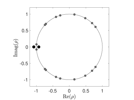
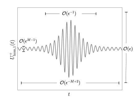
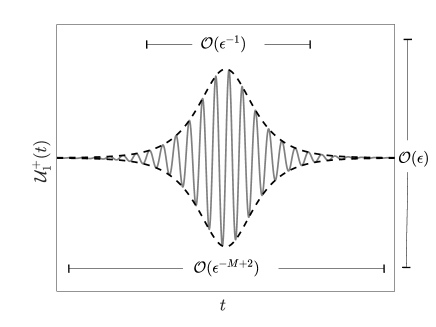
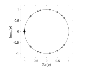
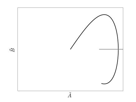
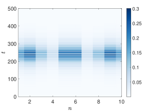
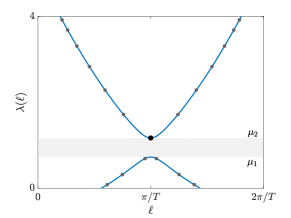
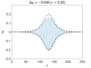
Before stating the main theorems of the paper, let us describe intuitively the generalized -gap breathers for . In the presence of time-periodic stiffness , some wavenumbers may fit into the gap in the dispersion relationship, as seen in Fig. 1(a). The corresponding Floquet multipliers are shown in panel (b) (details on the Floquet theory follow in Sec. 2). Unlike the situation for frequency gaps in (linear) spatially periodic media, exponential growth of Fourier modes occurs if the wavenumber is inside the gap of the dispersion relation since the Floquet exponent in the gap has positive real part, or equivalently, the Floquet multiplier has modulus exceeding unity. Due to this (parametric) instability, initializing Eq. (1) with such a Fourier mode will initially lead to growth. However, as the amplitude increases, the nonlinearity of the system comes into play, and, as we shall prove later, has a localizing affect on the dynamics, see Fig. 1(c). This solution, however, cannot decay to zero. This is due to the presence of neutrally stable modes (i.e., the Floquet multipliers lying on the unit circle). During the dynamic evolution, all of the Fourier modes will couple (due to the nonlinearity). The presence of the neutrally stable modes causes the small oscillations, as seen in the tails of Fig. 1(c). From a dynamical systems point of view, the trivial state has one unstable direction, one stable direction, and neutral directions. While genuine homoclinic solutions could be found in the intersection of the associated one-dimensional stable and unstable manifolds, it cannot be expected that such an intersection exists in an -dimensional phase space. Thus, only homoclinic solutions with small oscillating ripples for exist. These solutions lie in the intersection of the -dimensional center-stable manifold with the -dimensional center-unstable manifold of the origin, for which we use the time-reversibility of the system (1) with given by (5). The distance the wavenumber of the unstable Fourier mode is to the edge of the gap defines a small parameter (how exactly is detailed in Sec. 2). With normal form transformations for time-periodic systems (details in Secs. 3-6) it can be shown that the oscillating ripples can be made arbitrarily small, i.e., of order at the time scale of with some arbitrarily large but fixed, see Fig. 1(c). Using a multiple-scale analysis (details in Sec. 7), one can derive an explicit approximation of a genuine homoclinic orbit, see Fig. 1(d), which agrees with the leading order of the generalized breather’s profile.
We are now ready to present the main theorem on the existence of two homoclinic orbits with oscillating ripples, i.e., generalized -gap breathers. The assumptions (Spec) and (Coeff) are described in Secs. 2 and 5 respectively. The small parameter is defined in (Spec) and explicitly in the representation for .
Theorem 1.1.
Assume the spectral condition (Spec) and the normal form coefficient condition (Coeff) are satisfied. Then for every with there exists an and such that for all the system (1) with the time-periodic coefficient (5) and possesses two generalized homoclinic solutions satisfying
where satisfy and can be approximated as
where and are uniquely defined, real-valued functions with some , see Eq. (69) below.
In case of small damping each of the two homoclinic orbits of Theorem 1.1 breaks up. There exist two non-zero anti-periodic solutions with a -dimensional stable manifold for .
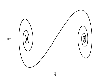
Therefore, as can be seen by counting the dimensions, the one-dimensional unstable manifold from the zero equilibrium intersects the -dimensional stable manifolds of one the two non-zero anti-periodic solutions transversally. In contrast to the oscillating homoclinic orbits, the heteroclinic orbits have no oscillating ripples as and converge to the orbits of the anti-periodic solutions as , see Figure 2.
Existence of the anti-periodic solutions is guaranteed by the following theorem.
Theorem 1.2.
The following theorem presents the main result on the existence of the heteroclinic orbits (transition fronts) between the trivial solution and the anti-periodic solutions .
Theorem 1.3.
Assume the spectral condition (Spec) and the normal form coefficient condition (Coeff). Fix . Then there exists an such that for all the system (1) with the time-periodic coefficient (5) and possesses two heteroclinic solutions such that
and
where are the anti-periodic solutions of (1) from Theorem 1.2.
Remark 1.4.
Because of the quadratic nonlinearity in the FPUT system (1), the homoclinic, anti-periodic, and heteroclinic orbits in Theorems 1.1-1.3 are not related by the sign reflection even though the leading orders obtained from the cubic normal form are related by the sign reflection, see Eq. (66). However, if , these orbits are related by the sign reflection up to any orders due to the symmetry of the FPUT system (1).
The article is organized as follows. Section 2 presents the Floquet and spectral analysis of the linearized FPUT system and introduce assumption (Spec). Preparations for the normal form transformations are described in Section 3. Normal form transformations are described in Section 4. The proof of Theorem 1.1 is given in Section 5, where assumption (Coeff) is introduced. Section 6 contains the proof of Theorems 1.2 and 1.3. A multiple-scale analysis is carried out in Section 7, which provides tractable approximations for both breathers and fronts. It also allows verification of (Coeff) through direct computation. Numerical illustrations of the main results are described in Section 8. Section 9 concludes the paper with a summary and brief discussions.
Funding: This work was partially supported by the National Science Foundation under grant number DMS-2107945 (C. Chong). D. E. Pelinovsky is partially supported by AvHumboldt Foundation as Humboldt Research Award. G. Schneider is partially supported by the Deutsche Forschungsgemeinschaft DFG through the cluster of excellence ’SimTech’ under EXC 2075-390740016.
2 The linearized system
The linearized FPUT system at the trivial (zero) equilibrium is given by
| (6) |
for with Dirichlet boundary conditions . The linearized system (6) is solved by a linear superposition of the discrete Fourier sine modes:
The -th Fourier mode has the amplitude for which the linear FPUT equation (6) transforms to the linear Schrödinger equation
| (7) |
where
and
We will review solutions of the spectral problem (7) by using the Floquet theory and the spectral theory of the Schrödinger operators.
2.1 Floquet theory
To obtain the monodromy matrix associated to (7) for general time-periodic coefficients , one may resort to numerical computation or perturbation analysis [26]. However, in the case of piecewise constant as in (5), this can be done explicitly [6, 37] (see also [7]). For the convenience of the readers, we summarize the relevant results.
Let for each , and define by
| (8) |
Note that also depend on but the index is dropped from the notation for simplicity. We obtain the exact solution of (7):
| (9) |
with some constants . By -continuity across , we obtain
| (10) |
The monodromy matrix is obtained as a mapping
| (11) |
with
| (20) |
Since and
| (21) |
the eigenvalues and of satisfies
with only three possibilities:
-
•
implies ,
-
•
implies with ,
-
•
implies .
The Floquet exponents of the mapping (11) are given by , where
-
•
implies ,
-
•
implies ,
-
•
implies .
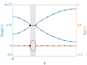
If , the trivial solution is spectrally stable if all Floquet exponents are purely imaginary. This corresponds to the case with . Figure 3(a) shows the Floquet multipliers in the critical case where with . The corresponding Floquet exponents are shown in Fig. 3(b).
(a)
 (b)
(b)
 (c)
(c)
2.2 Spectral theory
Let us review the spectral properties of the Schrödinger operator
with a -periodic coefficient in the particular case of . The spectrum of is purely continuous and consists of bands disjoint from each other by some gaps:
| (22) |
where are eigenvalues of with periodic boundary conditions and are eigenvalues of with anti-periodic boundary conditions . Eigenvalues correspond to of the Floquet theory, whereas eigenvalues correspond to and the spectral bands correspond to .
Remark 2.1.
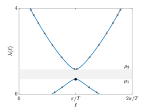
Note that is parameterized by the wavenumber in , which in turn determines the Floquet exponent . Within the spectral bands, the corresponding Floquet exponents are purely imaginary and are of the form . An example plot showing the dependence of on is shown in Fig. 3(c). For this example there is one band gap, which is the shaded region in the figure. The band gap edges are given by (the bottom of the gap) and (the top of the gap). This representation of the spectrum will be useful later when we derive an amplitude equation for the description of the envelope of the breather in Sec. 7. In particular, the concavity of will play a key role.
We define the bifurcation for a particular stiffness , for which , if there exists an integer such that coincides with the end point of and for are located inside . For the bifurcation shown in Figure 3, coincides with , for which the two bifurcating Floquet exponents are given by with . This bifurcation corresponds to and
| (23) |
Equivalently, we can obtain a bifurcation when coincides with with and
| (24) |
The two bifurcating Floquet exponents correspond to the Floquet multiplier at . All other Floquet exponents are assumed to be on the imaginary axis bounded away from and . The corresponding Floquet multipliers are on the unit circle bounded away from and .
2.3 Spectral assumption and defining the small parameter
With the linear theory in hand, we can now specify the spectral assumption as follows.
(Spec) There exists a periodic coefficient , for which all Floquet exponents lie on the imaginary axis. With the exception of two exponents at , they are assumed to be simple and non-zero. For small we assume that the two Floquet exponents at split symmetrically from the imaginary axis along the real axis to the order of .
We can define more explicitly by using the decomposition
| (25) |
where is a proper sign factor. For , the small parameter is related to the distance of the critical Floquet exponents from the imaginary axis in the following way. The real part of the Floquet exponent which depends on is given by
Since we know from (Spec) that with (for ), a series expansion of the real part of the Floquet exponent about yields , where we used the fact that and . In Sec. 7.2 we will show that
| (26) |
where is the corresponding band of at and the sign of is selected to be the opposite of the sign of .
Remark 2.2.
One can relate the small parameter to the distance of the bifurcating wavenumber to the band edge in the following way. For a fixed , suppose the wavenumber bandgap is , where the left edge and right edge depend on and can be found by solving trace() with . Suppose that the critical wavenumber coincides with the left band edge at the bifurcation point, (i.e., when ). Then, for , the distance to the band edge is . By inspection of (8) and (21), if one knows the critical values of and then can be determined by solving which yields
| (27) |
Thus .
3 Normal form transformations
The FPUT system (1) consists of oscillators with Dirichlet boundary conditions. By augmenting the vector with as the vector , we rewrite the -dimensional time-periodic system in the abstract form:
| (28) |
with the time-periodic coefficient matrix being piecewise continuous on for a period and the nonlinear function being smooth at with and . The solutions of the linear system
| (29) |
are, according to Floquet’s theorem, of the form
| (30) |
with a -time-periodic matrix function and a time-independent matrix , eigenvalues of which coincide with Floquet exponents in Section 2.
Remark 3.1.
Eigenvalues of the matrix are uniquely defined in the strip:
| (31) |
Eigenvalues of are generally complex-valued but we use the presentation (30) with real and real for convenience of the normal form transformations. For example, if are two complex-conjugate eigenvalues of , then the canonical form for the corresponding block of is
Remark 3.2.
As preparations for the normal form transformation, we can consider the time-periodic system (28) on the double period . The advantage of this approach is that the bifurcating Floquet exponents in the stripe (31) correspond to zero Floquet exponents in the -periodic system. The solution (30) of the linear system (29) can be rewritten in the form:
| (32) |
with the time-periodic matrix function and the time-independent matrix . According to the assumption (Spec) at the bifurcation point, has a double zero eigenvalue and all other (purely imaginary) eigenvalues of are simple and bounded away from .
Remark 3.3.
For the normal form transformation in Section 4 we need the following property of . Comparing the two representations of the fundamental matrix solution
we obtain
with being constant -matrices.
We now transform the system (28) on the double period to a convenient form for which the linear part is autonomous in . Let , then satisfies the time-periodic system:
| (33) |
We define the projection on the subspace associated with the double zero eigenvalue of by
| (34) |
where is a closed curve surrounding the origin in the plane counter-clockwise. The projection on the two other eigenvalues of on the imaginary axis is defined by . The range of is two-dimensional and the range of is -dimensional.
We apply these projections on system (33) and find for and that
| (35) | |||||
| (36) |
where we have introduced , ,
The splitting into is justified with . System (35)-(36) is extended by the additional equation , where is the bifurcation parameter in (Spec).
Remark 3.4.
In the context of the time-periodic system (33) on the double period, we recall that represents the modes associated to the two Floquet exponents which split from the double zero and leave the imaginary axis and that represents the modes associated to the other Floquet exponents which stay on the imaginary axis for small bifurcation parameter .
We use the normal form transformations to reduce the order of in terms of powers of .
Lemma 3.5.
Proof 3.6.
We set and then inductively
with being a -linear mapping in . After the transformations we have a system of the form
| (39) | |||||
| (40) |
with
and so . In order to have if we have to choose such that
| (41) |
where is the -linear part of , i.e. . Since
we also have to choose . Using Fourier series
it is easy to see that (41) can be solved w.r.t. since according to the assumption (Spec), none of the eigenvalues of are located at and has a double zero eigenvalue. As a result, the term can be made arbitrarily small in terms of powers of .
Remark 3.7.
The sequence of normal form transformations is not convergent and so we stop after transformations with some large but fixed , for which we have . Note that the minimum of is attained for -many transformations, after which is exponentially small in terms of , cf. [30].
4 Normal form transformations for the reduced system
If we ignore the terms in (37)-(38), then is an invariant subspace for (37)-(38). In this two-dimensional subspace the reduced system is obtained by setting in the first equation. So we consider the two-dimensional ODE
| (42) |
At the bifurcation point posseses a double eigenvalue with algebraic multiplicity two and geometric multiplicity one. Thus, we have a Jordan-block of size two. The eigenvector of is denoted with and the generalized eigenvector with , i.e. and . If we introduce coordinates , by
| (43) |
we can rewrite (42) as the following two-dimensional system
| (44a) | |||||
| (44b) | |||||
where and stand for real-valued nonlinear terms which are of the form
and similarly for , where and are independent of time. To simplify notations, we introduce here the normalized small parameter for the distance of the two Floquet exponents from the imaginary axis. According to the expansion (26), we have
| (45) |
For analyzing (44) we simplify this system by eliminating a number of terms by another normal form transformation
Lemma 4.1.
Proof 4.2.
It is well known that all terms which have a pre-factor which is oscillating in time can be eliminated by a normal form transform or equivalently by averaging, cf. [18, 40]. The technique is elaborated in the Normal Form Theorem III of [22, Theorem III.13]. For the quadratic terms there is no term which has a pre-factor which is constant in time and so all quadratic terms can be eliminated by a transformation
By suitably choosing the coefficients and we find
with new time-independent coefficients and . For simplifying the cubic terms we make a near identity transformation
Again by suitably choosing the coefficients and we find
with new coefficients and .
5 Proof of Theorem 1.1
Here we obtain the oscillating homoclinic solutions with small tails for . The bifurcating solutions scale as and , with . For the rescaled variables we find
| (46a) | |||||
| (46b) | |||||
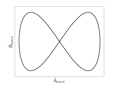
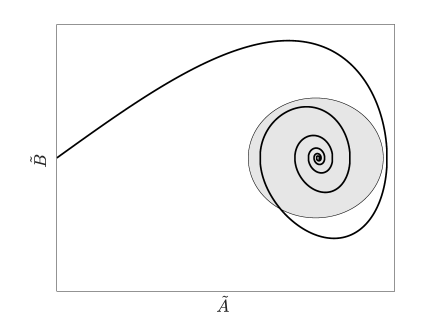
Ignoring the terms of order we find two homoclinic solutions to the origin, see the left panel of Figure 4, if the following sign condition holds.
(Coeff) Assume that
Remark 5.1.
Remark 5.2.
The truncated system (46), with terms neglected, admits an explicit solution
| (47) |
where and is to our disposal.
In the invariant subspace the homoclinic orbits persist in the reduced system (42) if the following reversibility condition holds.
(Rev) Assume that there exists such that .
Remark 5.3.
As a consequence of the reversibility, if is a solution, so is
Hence, the one-dimensional unstable manifold of the origin of the time -mapping transversely intersects the fixed space of reversibility and continue from the upper half to the lower half of the phase plane, see the right panel of Figure 4. Hence, by extending by its mirror picture at the fixed space of reversibility we constructed a homoclinic orbit
for the reduced system (44), where and with the leading-order solution given by (47). In the original variables the homoclinic orbit is denoted with and corresponds to the truncation for a given .
(a)
 (b)
(b)
The rest of this section contains the proof of Theorem 1.1, which we rewrite in notations of Sections 3 and 4 as follows.
Theorem 5.4.
Proof 5.5.
To prove persistence of if the terms are taken into account, we use again the reversibility. Obviously, it is impossible that the one-dimensional unstable manifold transversally intersects the -dimensional fixed space of reversibility for the full system (37)-(38). Therefore, it can only be expected that the homoclinic solutions persist as solutions with small tails for . This can rigorously be shown by intersecting the -dimensional center-unstable manifold with the fixed space of reversibility. Obviously this intersection is a transversal intersection.
On the center-unstable manifold the solutions converge towards the center manifold for with some exponential rate. However, the solutions on the center manifold can grow slowly, hence it remains to obtain bounds for such solutions. In a first step we apply another normal form transformation
to eliminate the bilinear terms which are linear in and linear in from the full system (37)-(38), where the
are bilinear mappings in their arguments. With some slight abuse of notation we skip the tildes and reconsider the system (37)-(38) but now with and additionally satisfying
The transformations are possible due to the spectral assumption (Spec).
In a second step we introduce the deviation from the homoclinic orbit by . The subsequent estimates on the deviation have already been carried out in a number of papers, cf. [17, 10]. We use the cutoff functions to estimate the solutions on with a suitable chosen large as .
The homoclinic orbit can be estimated pointwise by with a smooth . We denote the stable part of by and the projection on the stable part by . We find for a large determined below that
where
If the solution is in the fixed space of reversibility at we find
Summarizing the estimates yields
and so for and . This completes the proof of the theorem in view of the normal form transformations.
6 Proof of Theorem 1.2 and Theorem 1.3
Here we consider the case of small damping where reversibility no longer holds. For consistency of our analysis, we assume that with fixed. With the same analysis as for (44) and (46) we end up in at the reduced system for the rescaled variables which is now given by
| (48a) | |||||
| (48b) | |||||
where we used the expression for the Floquet exponents of the mapping (11) in Section 2.1. Ignoring the terms of order we first find two fixed points if . Since the fixed points are hyperbolic they persist as fixed points of the time--mapping even if the terms of order are included. This proves Theorem 1.2.
(a)
 (b)
(b)
Next we find two heteroclinic solutions connecting the origin with the two fixed points . In order to prove the persistence of these heteroclinic solutions we use that the one-dimensional unstable manifold of the origin transversely intersects the two-dimensional stable manifold of the two other fixed points of the reduced system. These heteroclinic solutions are shown on Figure 5.
To prove the persistence of heteroclinic solutions if the terms are taken into account we use that the stable manifold of the two other fixed points is -dimensional and so the one-dimensional unstable manifold of the origin transversally intersects the -dimensional stable manifold of the two anti-periodic solutions from Theorem 1.2. Theorem 1.3 is proven by using the transformations of Sections 3 and 4, with the decomposition .
7 Multiple-scale analysis and checking the assumption (Coeff)
For the system (1) with (2) we already checked the spectral condition (Spec) used in Theorems 1.1-1.3. Here we establish the validity of the normal form coefficient condition (Coeff).
We do so by formally deriving the reduced systems (46) and (48) via a multiple-scale analysis, which will yield an explicit and convenient formula for after adjusting the notations. Truncating (48) with terms neglected yields the scalar equation:
| (49) |
Remark 7.1.
The scalar equation (49) is recovered in Eq. (66) below with the correspondence between and given by (45). Note that the definition , see Eq. (43), is different from the definition , see Eq. (61) below. For Eq. (49), the amplitude is introduced based on the Floquet theorem, the decomposition into subspaces, and the normal form transformations. For Eq. (66), the amplitude is introduced directly by the perturbation expansions in powers of , see Eq. (60).
We define as in (25),
| (50) |
where is the potential for the bifurcation (23) or (24), is a small parameter for the asymptotic expansion, and is a proper sign factor.
7.1 Bloch modes of the unperturbed linear problem
We start with the linear problem for . In order to construct the asymptotic expansion, we define the Bloch function for the -th spectral band of , where . The parameter is defined in the Brillouin zone with and being at the ends of each spectral band corresponding to periodic and anti-periodic solutions respectively.
Let be the Hilbert space of -periodic functions with the inner product and the induced norm . The -normalized Bloch function is a -periodic solution of the spectral problem
| (51) |
which can be differentiated in as
| (52) |
and
| (53) |
Projecting to in yields from (52) and (53):
| (54) |
and
| (55) |
where the normalization condition has been used.
7.2 Perturbation of the linear problem
Let us consider asymptotic solutions of the linear equation
| (56) |
which follows from (7) and (50) at . As in (23), we take for which is selected in the first spectral band . The set-up for the second spectral band when as in (24) is essentially identical (see remark 7.3). Expanding
with and to be determined, we obtain for at the order of that
Since and , comparing with (52) yields
At the order of , we obtain the linear inhomogeneous equation,
| (57) |
Comparing (57) with (53) yields and if and only if , satisfies the amplitude equation
| (58) |
Alternatively, the amplitude equation (58) can be obtained by projecting the linear inhomogeneous equation (57) to in and using equations (54) and (55) with .
7.3 Perturbation of the nonlinear problem
Let us now consider asymptotic solutions of the nonlinear equation (1) with (50) and , where is fixed and . As in (23), we take , for which is selected in the first spectral band . To simplify computations, we will use expansions in terms of real-valued functions only. Expanding
| (60) |
we select the leading order in the form
| (61) |
where the amplitude is real according to (49) and the eigenfunction
| (62) |
is a real-valued, -anti-periodic solution of satisfying . At the order of we obtain
with
where and is the coefficient of the quadratic term in (1). In the explicit form, we obtain
with
The solution for can be written in the form
where and are solutions of the linear inhomogeneous equations:
| (63) | ||||
| (64) |
It follows from the linear theory that the real, -anti-periodic solution for exists in the form:
There exists a unique -periodic solutions for if and only if the non-resonance condition is met:
| (65) |
This non-resonance condition is satisfied if the spectral assumption (Spec) is satisfied.
By using Euler’s formulas, we obtain
and
Hence, we obtain
where we are only interested to write explicitly the coefficient for the bifurcating mode:
Projecting to gives the amplitude equation for :
| (66) |
where
| (67) |
and
| (68) |
Since the linear part of (66) should be identical to the linear amplitude equation (58), the new formula for must be identical to the previous equation (55) with . The expression for is defined in terms of real quantities only.
Remark 7.4.
Equation (66) for is analogous to the stationary NLS equation that can be derived in the context of spatially periodic media for the description of breathers [21]. A similar equation was derived in [34] for a (space-time continuous) photonic time crystal. Eq. (66) is equivalent to (49) with the correspondence (45) and the appropriate definitions of amplitudes and . The coefficient is constant proportional to .
Remark 7.5.
The coefficient in front of the second derivative in the amplitude equation (66) comes from an expansion of the imaginary parts of the spectral curves at the spectral gaps, see Fig. 3(c). The coefficient in front of the second derivative changes sign at every spectral boundary. Since the coefficient in front of the cubic coefficient in (66) does not change sign, the homoclinic and heteroclinic solutions exist as bifurcating solutions at every spectral gap associated with the anti-periodic eigenfunctions. In other words, if , then we pick the bifurcating mode at (23) with and . If , then we pick the bifurcating mode at (24) with and .
8 Comparison with numerical simulations
We now conduct a number of numerical simulations to illustrate the main results of the paper. We start with the simplest case, and work up in complexity.
Equation (66) with and has the following homoclinic solution
| (69) |
See Fig. 4(a) for an example plot of this solution in the phase plane. Returning to ansatz Eq. (60), we have the following leading order approximation in terms of the original lattice variables,
| (70) |
To make practical use of this approximation, the first step is to identify the bifurcation value (namely the critical modulation amplitude values and ) and critical mode number such that where is the monodromy matrix defined in Eq. (20). This corresponds to the bifurcation scenario shown in Fig. 3. In this case, the Floquet exponent corresponding to will be purely imaginary and will be of the form . The corresponding Bloch mode is obtained by solving Eq. (51). This can be done explicitly, see Sec. 2.1 or the appendix of [7] for details. Next, we compute using Eq. (55) with which depends only on and its derivatives, which can also be computed explicitly. Equivalently, one can determine using Eq. (67).
8.1 Examples with and
The nonlinear coefficient can be computed from if , i.e., if there is no quadratic nonlinearity (the case of is discussed below). To compute in this case, we substitute into Eq. (68) and evaluate.
As our first example, we chose parameters that correspond to the spectral picture in Fig. 3 and and . In this case the critical mode lies at the top of the first spectral band, namely . This demonstrates that the spectral condition (Spec) is satisfied and we choose . It can be seen from Fig. 3(c), or via direct calculation, that . By choosing , we have that , and thus (Coeff) is satisfied.
(a)
 (b)
(b)
 (c)
(c)
To generate the generalized -gap breather, we keep all parameters fixed, but select and , . With these parameter values, the mode lies in the spectral gap. The corresponding Floquet multipliers and exponents and are shown in Fig. 1(a,b). We initialize the numerical simulation with
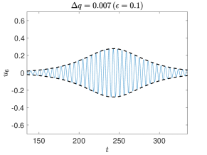
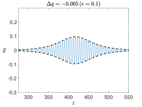
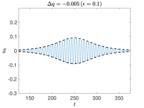
For initial data with such small amplitude, the dynamics will initially be nearly linear, and hence the solution will grow exponentially with rate given by Re(), which is the real part the Floquet exponent associated to mode (see the larger black dot in Fig. 1(a)). According to Eq. (58), an approximation of this growth rate is given by (59) with . As the amplitude increases in the dynamic evolution, the affect of the nonlinearity comes into play, which will cause the solution to experience decay, such that the resulting waveform is localized in time. The time series of the node is shown in Fig. 6(a). The temporal localization occurs uniformly throughout the lattice, as seen in the intensity plot of Fig. 6(b). By construction, the wavenumber lies in a wavenumber bandgap. Thus, the solution shown in Fig. 6(a,b) is a generalized -gap breather. The analytical prediction based on Eq. (70) is shown as the dashed-line in panel (a). For the sake of clarity, only the envelope of the approximation is shown, which is simply a plot of the local maximums (and minimums) of Eq. (70).
(a)
 (b)
(b)
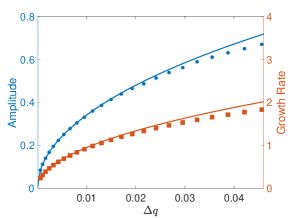
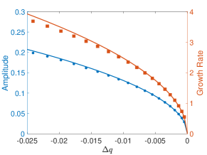
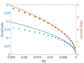
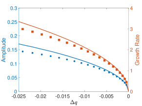
For , the distance of the wavenumber to the edge of the gap is , where is the wavenumber at the (left) edge of the gap. Recall from Eq. (27) that . Since the amplitude of the breather is , see Eq. (70), the amplitude grows like . This observation was made numerically and experimentally in [7], which we have now proved. This amplitude trend is consistent with the trend found for discrete breathers in space-periodic systems where it is well known that the breather amplitude grows like , where is the difference between the breather frequency and the edge of the frequency spectrum [12]. Using (27) and Eq. (70) allows us to obtain an analytical prediction of the breather amplitude dependence of the distance to the band edge, see Fig. 6(c). For small values of (and hence ) the agreement is very good. The growth parameter gives an indication of how wide or narrow the breather will be, with larger growth parameters corresponding to narrower solutions. The prediction from the linear theory is given by the real part of the Floquet exponent corresponding to mode , and the approximation from the perturbation analysis is (59). A comparison of these two quantities are shown as the red markers and lines, respectively of Fig. 6(c). The trends in Fig. 6(c) demonstrate that the -gap breathers becomes larger in amplitude and more narrow as the wavenumber goes deeper into the gap.
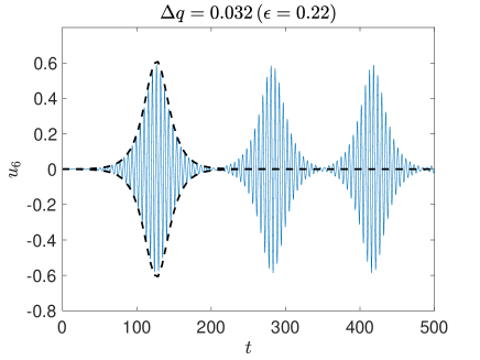
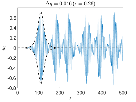
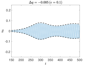
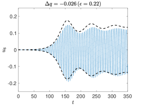
In Fig. 6(c) the -gap breathers are generated up until (which corresponds to ). For , the width of the wavenumber bandgap is (where , are the right and left edges of the bandgap, respectively). Thus, the branch of solutions shown Fig. 6(c) extends to roughly 15% of the width of the bandgap. For we did not observe a coherent temporal localization. Indeed, for all the breathers observed numerically, the localization is obtained for a finite interval of time. For longer time simulations the amplitude of the breather can grow again (leading to a repeated appearance of breathers), see Fig. 7(a). Similar observations have been made for k-gap solitons in photonic systems [34]. While Theorem 1.1 guarantees that a temporally localized structures exists over a finite temporal interval, there is no statement about the dynamics beyond this interval. The numerical simulations suggest the tail of the breather can experience repeated growth. We observed as becomes larger, the time between consecutive peaks of the pulses becomes smaller. In other words, the emergence of the “second” breather occurs faster as becomes larger. Thus, for sufficiently large the structure is not temporally localized since the second breather emerges “too soon”, see Fig. 7(b). This is the reason why we only show in Fig. 6(c).
(a)
 (b)
(b)
 (c)
(c)
Next, we consider an example where the breathers bifurcate from . The spectral bands corresponding to , , , and are shown in Fig. 8(a). For these parameter values the mode lies at the bottom of the second spectral band, namely . Notice that the concavity of the second spectral band is opposite of the first band, namely . Thus, in order to satisfy the (Coeff) condition, we require . If this implies that and the sign parameter is now Thus, for the next numerical simulations, we fix and The approximation given in Eq. (70) is identical in this case, but we replace with , and likewise for the underlying Bloch modes (where should be replaced by , etc.).
Figure 8(b) shows an example of the generalized -gap breather with , with corresponding envelope prediction given by Eq. (70). Qualitatively, the results are similar to the example shown in Fig. 6(a). Figure 8(c) shows the dependence of the breather amplitude and growth rate on the parameter . Note, since the breather is bifurcating from the right edge of the wavenumber bandgap, the quantity will be negative. The breather amplitude grows like .
8.2 Examples with and
Here we will consider . In particular, we will chose values of the nonlinear coefficients in (4) that correspond to the modulated magnetic lattice described in Sec. 1.1 so that the results obtained here are directly relevant for the experimental set-up described in [7]. In the re-scaled variables the interaction coefficients are and . Since the sign of must be computed directly to see if the relevant eigenvalue to bifurcate from is or . will depend on the function , which we can obtain by solving Eq. (64). It will be convenient to estimate numerically under the constraint that is periodic, which we achieve using a shooting method. In particular, we apply Newton iterations on the map where is the solution of Eq. (64) with initial condition . The Jacobian of the map is simply , where is the 2x2 identity matrix and is the solution to the variational equation with initial value where is the Jacobian corresponding to Eq. (64) [20].
(a)
 (b)
(b)
 (c)
(c)
In this example, we consider the spectral situation as shown in Fig. 8(a), such that is the critical mode bifurcating from . In this case, , so we chose and we must have to satisfy (Coeff). Upon computing with the shooting method and substituting into Eq. (68) with and we find , as desired.
Figure 9(a) shows a numerical simulation of the lattice with initial displacement and , and panel (b) shows a simulation with . By comparing panels (a) and (b), we see once again that the -gap breather becomes more narrow and larger in amplitude as (and thus ) increases in magnitude. What is also apparent, especially in panel (b), is that the numerical simulation is asymmetric, namely, the maximum is not simply the minimum reflected about the line. Evidently, the asymmetric nature of the FPUT potential with is manifested through a lack of reflection symmetry in the -gap breather profile. Asymmetric breathing profiles are well known in space-periodic FPUT systems with quadratic nonlinearities [21]. The approximation given by Eq. (70) remains symmetric, however, and thus one would expect the approximation not to do as well as in the case. Indeed, inspection of Fig. 8(c) confirms this, where the difference in amplitude between simulation and theory is larger than in the case (see e.g., Fig. 8(c)). Nonetheless, the asymptotic behavior as is correct, and in particular the breather amplitude grows like .
8.3 Examples with and
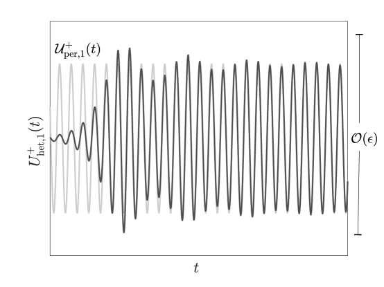
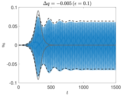
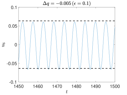
In our final example, we include the effect of damping and select . By definition, , so the critical parameter set (when ) will have , like before. Thus, we consider once again the parameter set that corresponds to Fig. 9(a). However, the numerical solutions and asymptotic approximations will have non-zero damping affect for . Since the bifurcation scenario is the same as in Fig. 9(a) the initial condition for simulations will be of the same form, namely . An example lattice simulation with is shown in Fig. 10(a) where the underlying damping constant is . The solution experiences an initial growth, with growth rate given by the real part of the Floquet exponent, but rather then decaying to a near zero amplitude, like in all the previous examples with , the solution approaches steady periodic motion with period . A longer time evolution of the same solution is shown in Fig. 11. In particular, panel (b) shows the dynamics are essentially periodic for sufficiently larger.
In terms of the Poincaré map , the trivial solution is clearly a fixed point. The -periodic solution that is approached in the dynamic simulation is another fixed point. Thus, the solution shown in Fig. 10(a) is a transition front, since it connects two different fixed points.
Another example of the transition front for a larger value of is shown in Fig. 10(b). Despite the fact that the structure is not temporally localized, the initial dynamics still resemble the “left” side of the -gap breather. Indeed, the homoclinic approximation from Eq. (70) is quite close to the initial front dynamics (see the solid gray line of Fig. 10(a)). For this reason, it is still reasonable to measure the amplitude of the front in the same way we measured the amplitude for the -gap breathers. A plot of the front amplitude and real part of the Floquet exponent is shown in 10(c). The amplitude trend is similar to the non-damped case, but the magnitude of the amplitude is smaller, as expected (compare panel (c) of Figs. 9 and 10).
(a)
 (b)
(b)
 (c)
(c)
(a)
 (b)
(b)
The amplitude equation Eq. (66) can be used to approximate the front dynamics. However, the equation does not yield an explicit solution in the presence of damping and so we will employ a qualitative and numerical analysis of Eq. (66). A straightforward phase plane analysis shows that the trivial fixed point is a saddle with corresponding eigenvalues and the fixed points are spiral-sinks with corresponding eigenvalues where the are the coefficients of Eq. (66), namely,
In the phase plane, there is a heteroclinic orbit that leaves the trivial fixed point along the unstable eigenvector and approaches the fixed point. There is another heteroclinic orbit that leaves the trivial fixed point along the unstable eigenvector and approaches the fixed point, see Fig. 5. To approximate the heteroclinic orbit, we numerically solve Eq. (66) with initial condition . The resulting solution is then used in Eq. (60) to generate the approximation of the lattice dynamics.
Examples are shown in Fig. 10(a,b), where the envelopes are shown for and , respectively. Once again, the envelope dynamics are captured well by Eq. (60), especially for small . The periodic oscillation of the envelope can be approximated by the imaginary part of the eigenvalue associated to the non-trivial fixed point, namely . In terms of the original lattice variables this translates to . For the example shown in Fig. 11(a) with , the average peak-to-peak time of the envelope is time units, where as , which is quite close.
The front amplitude as a function of is shown as the solid blue line in panel (c), and an approximation of the initial growth rate is shown as the red line. Once again the asymptotic behavior as is correct. Despite the presence of damping, the front amplitude grows like .
9 Conclusions
Generalized -gap breathers are coherent structures that are localized in time, periodic in space, and have wavenumber in a -gap. They are the natural counterpart of the discrete breathers of spatially periodic lattices, which themselves are of fundamental importance in a diverse range of fields.
In the absence of damping, we proved rigorously the existence of generalized -gap breathers in a time-periodic FPUT lattice using normal form theory. In particular, we proved the existence of oscillating homoclinic solutions over a finite time interval with tails that can be made arbitrarily small, but finite. These solutions bifurcate from one edge of the -gap. Which of the edges is determined by the nonlinear coefficients and the concavity of the spectral band from which the solution bifurcates. The amplitude of the -gap breather grows like , where is the distance of the underlying wavenumber to the band edge. This result makes rigorous the numerical and experimental observations of such -gap breathers in [7]. We also provided a tractable analytical approximation of such solutions using a multiple-scale analysis and corroborated results with direct numerical simulations.
In the presence of damping we proved the existence of solutions that connect the zero state to a time-periodic one, which we called the transition fronts. The multiple-scale analysis also provided an accurate description of the front solutions, although the underlying amplitude equation needed to be solved numerically. The initial stage of the front dynamics were well described by the undamped -gap breather approximations.
Generalized -gap breathers and transition fronts represent new types of nonlinear wave structures. This work provided the first rigorous results in their study, complementing earlier experimental and numerical work. Nonetheless, there are still many open questions regarding -gap breathers and transition fronts. This includes the possible existence of genuine -gap breathers (i.e., with both tails decaying to zero), the numerically exact computation of -gap breathers (i.e., numerical roots of the appropriate map up to a user-prescribed tolerance) and the exploration of such structures in higher spatial dimensions or in settings beyond the FPUT realm. Indeed, any system that is already described by a nonlinear wave equation that could be adapted to be time-varying (in order to induce a -gap) would be a candidate for the implementation of -gap breathers. This suggests that -gap breathers’ relevance, and hence the results of this work, could extend to a wide range of fields.
References
- [1] N. Akhmediev, A. Ankiewicz, and J. M. Soto-Crespo, Rogue waves and rational solutions of the nonlinear Schrödinger equation, Phys. Rev. E, 80 (2009), p. 026601.
- [2] A. Ankiewicz, N. Akhmediev, and J. M. Soto-Crespo, Discrete rogue waves of the Ablowitz-Ladik and Hirota equations, Phys. Rev. E, 82 (2010), p. 026602.
- [3] G. P. Berman and F. M. Izrailev, The fermi-pasta-ulam problem: Fifty years of progress, Chaos, 15 (2005).
- [4] M. Butt, S. Khonina, and N. Kazanskiy, Recent advances in photonic crystal optical devices: A review, Optics and Laser Technology, 142 (2021), p. 107265.
- [5] L. S. Cao, D. X. Qi, R. W. Peng, M. Wang, and P. Schmelcher, Phononic frequency combs through nonlinear resonances, Phys. Rev. Lett., 112 (2014), p. 075505.
- [6] M. Centurion, M. A. Porter, Y. Pu, P. G. Kevrekidis, D. J. Frantzeskakis, and D. Psaltis, Modulational instability in nonlinearity-managed optical media, Phys. Rev. A, 75 (2007), p. 063804.
- [7] C. Chong, B. Kim, E. Wallace, and C. Daraio, Modulation instability and wavenumber bandgap breathers in a time layered phononic lattice, Phys. Rev. Research, 6 (2024), p. 023045.
- [8] T. Dauxois, Fermi, Pasta, Ulam, and a mysterious lady, Phys. Today, 61(1) (2008), p. 55.
- [9] S. V. Dmitriev, E. A. Korznikova, Y. A. Baimova, and M. G. Velarde, Discrete breathers in crystals, Physics-Uspekhi, 59 (2016), pp. 446–461.
- [10] T. Dohnal, D. E. Pelinovsky, and G. Schneider, Travelling modulating pulse solutions with small tails for a nonlinear wave equation in periodic media, Nonlinearity, 37 (2024), p. 055005.
- [11] E. Fermi, J. Pasta, S. Ulam, and M. Tsingou, Studies of nonlinear problems i, 1955.
- [12] S. Flach and A. Gorbach, Discrete breathers: advances in theory and applications, Phys. Rep., 467 (2008), p. 1.
- [13] S. Flach, M. V. Ivanchenko, and O. I. Kanakov, -Breathers and the Fermi-Pasta-Ulam Problem, Phys. Rev. Lett., 95 (2005), p. 064102.
- [14] R. Fukuizumi and G. Schneider, Interchanging space and time in nonlinear optics modeling and dispersion management models, J. Nonlinear Sci., 32 (2022), pp. 29, 39.
- [15] G. Gallavotti, The Fermi–Pasta–Ulam Problem: A Status Report, Springer-Verlag, Berlin, Germany, 2008.
- [16] A. Ganesan, C. Do, and A. Seshia, Phononic frequency comb via intrinsic three-wave mixing, Phys. Rev. Lett., 118 (2017), p. 033903.
- [17] M. D. Groves and G. Schneider, Modulating pulse solutions for quasilinear wave equations, Journal of Differential Equations, 219 (2005), pp. 221–258.
- [18] J. Guckenheimer and P. Holmes, Nonlinear oscillations, dynamical systems, and bifurcations of vector fields, vol. 42 of Appl. Math. Sci., Springer, Cham, 1983.
- [19] W. Hartmann, Acoustic Signal Processing, Springer New York, New York, NY, 2007, pp. 503–530.
- [20] M. Hirsch, S. Smale, and R. Devaney, Differential Equations, Dynamical Systems, and an Introduction to Chaos, Pure and Applied Mathematics - Academic Press, Elsevier Science, 2004.
- [21] G. Huang and B. Hu, Asymmetric gap soliton modes in diatomic lattices with cubic and quartic nonlinearity, Phys. Rev. B, 57 (1998), p. 5746.
- [22] G. Iooss and M. Adelmeyer, Topics in bifurcation theory and applications., vol. 3 of Adv. Ser. Nonlinear Dyn., Singapore: World Scientific, 2nd ed. ed., 1998.
- [23] P. G. Kevrekidis, Non-linear waves in lattices: Past, present, future, IMA J. Appl. Math., 76 (2011), pp. 389–423.
- [24] B. L. Kim, C. Chong, S. Hajarolasvadi, Y. Wang, and C. Daraio, Dynamics of time-modulated, nonlinear phononic lattices, Phys. Rev. E, 107 (2023), p. 034211.
- [25] B. L. Kim, C. Daraio, C. Chong, S. Hajarolasvadi, and Y. Wang, Dynamics of time-modulated, nonlinear phononic lattices, arxiv:, (2022), p. 2209.06511.
- [26] I. Kovacic, R. Rand, and S. M. Sah, Mathieu’s equation and its generalizations: Overview of stability charts and their features, Applied Mechanics Reviews, 70 (2018).
- [27] A. B. Kozyrev, H. Kim, and D. W. van der Weide, Parametric amplification in left-handed transmission line media, Applied Physics Letters, 88 (2006), p. 264101.
- [28] G. Lee, D. Lee, J. Park, Y. Jang, M. Kim, and J. Rho, Piezoelectric energy harvesting using mechanical metamaterials and phononic crystals, Commun Phys, 5 (2022), p. 94.
- [29] L. Liu, W.-R. Sun, B. A. Malomed, and P. G. Kevrekidis, Time-localized dark modes generated by zero-wave-number-gain modulational instability, Phys. Rev. A, 108 (2023), p. 033504.
- [30] E. Lombardi, Orbits homoclinic to exponentially small periodic orbits for a class of reversible systems. Application to water waves, Arch. Ration. Mech. Anal., 137 (1997), pp. 227–304.
- [31] J. Marconi, E. Riva, M. Di Ronco, G. Cazzulani, F. Braghin, and M. Ruzzene, Experimental Observation of Nonreciprocal Band Gaps in a Space-Time-Modulated Beam Using a Shunted Piezoelectric Array, Physical Review Applied, 13 (2020), p. 031001.
- [32] S. Mukherjee and M. C. Rechtsman, Observation of unidirectional solitonlike edge states in nonlinear floquet topological insulators, Phys. Rev. X, 11 (2021), p. 041057.
- [33] H. Nassar, B. Yousefzadeh, R. Fleury, M. Ruzzene, A. Alù, C. Daraio, A. N. Norris, G. Huang, and M. R. Haberman, Nonreciprocity in acoustic and elastic materials, Nature Reviews Materials, 5 (2020), p. 667–685.
- [34] Y. Pan, M.-I. Cohen, and M. Segev, Superluminal -gap solitons in nonlinear photonic time crystals, Phys. Rev. Lett., 130 (2023), p. 233801.
- [35] D. A. Powell, I. V. Shadrivov, and Y. S. Kivshar, Multistability in nonlinear left-handed transmission lines, Applied Physics Letters, 92 (2008), p. 264104.
- [36] , Asymmetric parametric amplification in nonlinear left-handed transmission lines, Applied Physics Letters, 94 (2009), p. 084105.
- [37] Z. Rapti, G. Theocharis, P. G. Kevrekidis, D. J. Frantzeskakis, and B. A. Malomed, Modulational instability in bose–einstein condensates under feshbach resonance management, Physica Scripta, 2004 (2004), p. 27.
- [38] J. R. Reyes-Ayona and P. Halevi, Observation of genuine wave vector ( or ) gap in a dynamic transmission line and temporal photonic crystals, Applied Physics Letters, 107 (2015), p. 074101.
- [39] M. Safaei, H. A. Sodano, and S. R. Anton, A review of energy harvesting using piezoelectric materials: state-of-the-art a decade later (2008–2018), Smart Materials and Structures, 28 (2019), p. 113001.
- [40] J. A. Sanders, F. Verhulst, and J. Murdock, Averaging methods in nonlinear dynamical systems, vol. 59 of Appl. Math. Sci., New York, NY: Springer, 2nd ed. ed., 2007.
- [41] M. Soljačić, M. Ibanescu, S. G. Johnson, Y. Fink, and J. D. Joannopoulos, Optimal bistable switching in nonlinear photonic crystals, Physical Review E, 66 (2002), p. 055601.
- [42] G. Trainiti, Y. Xia, J. Marconi, G. Cazzulani, A. Erturk, and M. Ruzzene, Time-Periodic Stiffness Modulation in Elastic Metamaterials for Selective Wave Filtering: Theory and Experiment, Physical Review Letters, 122 (2019), p. 124301.
- [43] A. Vainchtein, Solitary waves in fpu-type lattices, Physica D, 434 (2022), p. 133252.
- [44] F. Y. Wang, G. X. Li, H. L. Tam, K. W. Cheah, and S. N. Zhu, Optical bistability and multistability in one-dimensional periodic metal-dielectric photonic crystal, Applied Physics Letters, 92 (2008), p. 211109.
- [45] C.-P. Wen, W. Liu, and J.-W. Wu, Tunable terahertz optical bistability and multistability in photonic metamaterial multilayers containing nonlinear dielectric slab and graphene sheet, Applied Physics A, 126 (2020), p. 426.
- [46] M. Yu, J. K. Jang, Y. Okawachi, A. G. Griffith, K. Luke, S. A. Miller, X. Ji, M. Lipson, and A. L. Gaeta, Breather soliton dynamics in microresonators, Nature Communication, 8 (2017), p. 14569.