Nonlinear studies of modifications to general relativity: Comparing different approaches

Abstract

Studying the dynamical, nonlinear regime of modified theories of gravity remains a theoretical challenge that limits our ability to test general relativity. Here we consider two generally applicable, but approximate methods for treating modifications to full general relativity that have been used to study binary black hole mergers and other phenomena in this regime, and compare solutions obtained by them to those from solving the full equations of motion. The first method evolves corrections to general relativity order by order in a perturbative expansion, while the second method introduces extra dynamical fields in such a way that strong hyperbolicity is recovered. We use shift-symmetric Einstein-scalar-Gauss-Bonnet gravity as a benchmark theory to illustrate the differences between these methods for several spacetimes of physical interest. We study the formation of scalar hair about initially non-spinning black holes, the collision of black holes with scalar charge, and the inspiral and merger of binary black holes. By directly comparing predictions, we assess the extent to which those from the approximate treatments can be meaningfully confronted with gravitational wave observations. We find that the order-by-order approach cannot faithfully track the solutions when the corrections to general relativity are non-negligible. The second approach, however, can provide consistent solutions, provided the ad-hoc timescale over which the dynamical fields are driven to their target values is made short compared to the physical timescales.

I Introduction

Remarkably, the theory of general relativity (GR) has passed all experimental and observational tests to date Will (2014), including on cosmological Clifton et al. (2012) and short scales Lee et al. (2020); Kapner et al. (2007), in slow-motion, weak-curvature Abuter et al. (2020) and strong-curvature Kramer et al. (2021); Akiyama et al. (2019, 2022); Völkel et al. (2021); Psaltis et al. (2020); Kocherlakota et al. (2021) regimes, as well as in the nonlinear, high-velocity, strong-field regime Abbott et al. (2016a); Yunes et al. (2016); Baker et al. (2017); Isi et al. (2019, 2020); Okounkova et al. (2022); Abbott et al. (2019a, b, 2020, 2021a). The last-named has been probed, in recent years, through the gravitational wave (GW) observations of compact object binary mergers by the LIGO, Virgo and KAGRA detectors Aasi et al. (2015); Acernese et al. (2015); Somiya (2012); Aso et al. (2013). In general, tests of GR with GW observations fall into two categories: those that look for generic types of deviations from GR, and those that target specific theories. The former assumes the underlying gravitational signal is well described by GR (potentially adding independent parametric deviations to the signal, whether for the inspiral, the merger or the ringdown stages, to characterize potential deviations) Abbott et al. (2019a, b, 2021b, 2021a); Ghosh (2022). However, in general, a consistent modified theory will introduce deviations in a more complicated and correlated manner, which such tests may be insensitive to. Even when such searches are sensitive, there could be subtleties in trying to map constraints on parameteric deviations to constraints on parameters in specific theories related to the choice of priors and the actual parameters on which the measurements are done. Example predictions from specific theories could be used to test, improve, and motivate new generic tests. They could also be directly compared to the data, in principle allowing us to place the most stringent constraints on deformations of GR Yunes and Siemens (2013); Berti et al. (2015, 2018a, 2018b). However, in order to make predictions of the GW signals from the final stages of compact object mergers to compare to the observations, solutions in beyond GR theories are required.

There are a number of challenges associated with studying compact object mergers in modified theories, the foremost of which is that in any theory that modifies the principal part of the Einstein equations, the issue of a well-posed initial value problem must be revisited. In order to address this issue, several strategies have emerged in the literature for simulating compact object mergers in modified theories:

1. Focus on specific modified theories where a formulation leading to well posed initial value problem is known (at least for some range of parameters), and solve the full evolution equations.

2. Exploit the observation that corrections to GR ought to be subleading, and incorporate their effects on the dynamics in a perturbative fashion, order by order, where corrections are evaluated with respect to the solution obtained at lower order, thereby maintaining the same principal structure as in GR.

3. Take the effective field theory (EFT) viewpoint that a modified theory is only valid up to some short length/timescale, and “fix" the evolution equations below this scale by introducing new dynamical fields that replace high derivative terms in the original evolution equations, allowing them to maintain the same principal structure as in GR, while including the effect of correcting terms via suitable coupling among relevant fields. These new fields are given evolution equations that drive them to the values they would have in the original theory on some short timescale.

We expound on these different strategies below.

Applications of approach (i), solving the full evolution equations, have mostly focused on theories with second order equations of motion. (Though it should be noted that some special theories with higher than second order equations of motion can still be well-posed and evolved nonlinearly. An example of this is quadratic gravity, which gives fourth order equations Noakes (1983); Held and Lim (2021, 2023); East and Siemonsen (2023).) In this case, at sufficiently weak coupling, the modified theory can be seen as having the principal part one would have in GR, with some small correction. Crucially, even at weak coupling such modifications can lead to the loss of well-posedness when using standard formulations of the equations of motion. For example, generic examples of Horndeski theories—scalar-tensor theories with second order equations of motion—do not lead to well posed problems in the harmonic formulation Papallo and Reall (2017) (as the resulting equations of motion are weakly, but not strongly hyperbolic). However, general Horndeski theories have been shown to lead to a (locally) well-posed initial value problem in a modified generalized harmonic (MGH) formulation Kovacs and Reall (2020a, b), so long as the length scale associated with the beyond-GR coupling is much smaller than all the other length scales in the problem. (At larger couplings, such theories can exhibit the complete breakdown of hyperbolicity, e.g. Ripley and Pretorius (2019a); Bernard et al. (2019).) The MGH formulation has been used to simulate compact object mergers and compute GW signals in example modified theories East and Ripley (2021a, b); East and Pretorius (2022); Corman et al. (2023), and has been extended to the modified CCZ4 formulation Aresté Saló et al. (2022, 2023). Related to this are studies of compact object mergers in Horndeski theories where the metric evolution can be treated the same way as in GR, but the principal part of the scalar field evolution is modified from that of the wave equation Figueras and França (2022); Bezares et al. (2022). With this approach, the dynamics of binary black holes and other compact object mergers can be studied, and predictions for the resulting GW signals can be extracted, without approximation (beyond that of numerical discretization error), at least within some range of the parameter space of theories where a well-posed formulation is known. However, there exist many classes of modified gravity theories which almost certainly define ill-posed problems if treated as complete theories, regardless of the value that the coupling parameter controlling the modifications. Taking an EFT perspective, this can be seen as a natural consequence of a specific truncation of the theory. In order to treat such theories, a different strategy, making use of the perturbative nature of the modifications to GR, is necessary.

Approach (ii), the order-by-order approach, treats mathematical pathologies in modified theories by evolving separately the corrections to GR at each order (in the coupling controlling the modifications to GR) and only evaluating corrections through solutions to previous orders. Backreaction of corrections to the GR solution are thus only passively and perturbatively accounted for through higher order corrections to the solution, ensuring the principal part of the equations is unaltered. For example, and focusing primarily on the two body problem, studies of dynamical Chern Simons gravity Alexander and Yunes (2009) and Einstein scalar Gauss Bonnet (EsGB) gravity (discussed below) have been pursued using this strategy to solve for the leading order correction to the metric Okounkova et al. (2017, 2019a, 2020); Okounkova (2020). However, the quality (or faithfulness) of the solutions that are obtained depends not only on the corrections being small, but also on secular effects due to the accumulation of errors introduced at the perturbative order staying small. In the inspiral of a binary black hole, strong secular effects accumulate in the order-by-order approach on the radiation-reaction timescale Okounkova et al. (2020); Okounkova (2020), making it unclear what parts of the computed GW signal can accurately be extracted from such a computation.

An alternative approach is fixing the equations (iii), where extra fields are introduced in a way that mocks up degrees of freedom that would have been integrated out in an EFT truncation in such a way that they play a subleading role in the dynamics. An ad-hoc prescription is used to drive these fields towards satisfying specific identities on a certain chosen time/lengthscale, while modes below this scale are effectively damped away. As a consequence of replacing higher order terms with these extra fields, well posedness is achieved. Correcting terms actively backreact, and are treated consistently within the approximation in the limit of the prescription’s timescale is much smaller than the other physical timescales in the problem. Obtaining quality solutions this way requires that the ad-hoc timescale be made short compared to the other physical timescales, and that the dynamics does not lead to a significant UV cascade, so that the solution is not sensitive to the ad-hoc scale. For instance, an EFT which introduces higher order modifications to GR without new fields Endlich et al. (2017) was studied in recent works Cayuso and Lehner (2020); Lara et al. (2022); Franchini et al. (2022); Bezares et al. (2022). Assessing whether one can obtain an answer that is insensitive to the fixing scale for the problem of interest is essential to being able to draw physical conclusions and examine the viability of the theory under study. In some cases, this may pose a practical challenge, as simulating compact object mergers is computationally expensive, and this approach, by construction, introduces an additional small scale that must be resolved.

The goal of this study is to focus on binary black hole mergers in a benchmark modified gravity theory where the full equations can be solved [approach (i)], and employ such solutions to evaluate the order-by-order approach (ii) and the fixing-the-equations approach (iii). (As well, all solutions can be compared to those in GR for comparable physical parameters). In Ref. Allwright and Lehner (2019), a comparison between these three approaches was carried out for a scalar field toy-model with a known UV completion, highlighting some of the clear shortcomings of the order-by-order strategy, while in Ref. Franchini et al. (2022), spherically-symmetric scalar field collapse in EsGB was studied using approaches (i) and (iii). Here we study specifically the case of binary black hole dynamics. As binary black holes in GR do not display a significant UV-cascade Allwright and Lehner (2019) and solutions remain smooth throughout, it could be argued that corrections in a modified theory likely remain small, and potentially all approaches could be useful. By leveraging full solutions of binary black hole mergers, we are able to directly quantify the errors introduced by secular effects in the order-by-order approach and by different prescriptions for the ad-hoc dynamical fields with non-zero damping timescales in the fixing-the-equations approach, in order to study their accuracy.

The particular benchmark theory we will focus on is shift-symmetric EsGB gravity. This theory introduces deviations from GR at small curvature length scales and yields solutions that are distinct from those in GR. Indeed, vacuum black holes evolve to develop stable scalar clouds Kanti et al. (1998); Yunes and Stein (2011); Sotiriou and Zhou (2014a, b), and hence can differ qualitatively from GR in the strong field regime, while still passing weak field tests. EsGB is thus a promising theory to perform theory-specific tests of GR in the strong field, dynamical regime. From a theoretical point of view, shift-symmetric EsGB gravity can be motivated as the leading order scalar-tensor theory of gravity whose resulting equations of motion are invariant under a shift in the scalar field. As a result, significant recent work has gone into modeling compact object mergers in EsGB gravity both in post-Newtonian Yagi et al. (2012); Sennett et al. (2016); Shiralilou et al. (2021a, b); van Gemeren et al. (2023); Julié et al. (2023); Julié (2023) and numerical relativity using either approach (i) East and Ripley (2021a, a); Ripley (2022); East and Pretorius (2022); Corman et al. (2023); Aresté Saló et al. (2022, 2023) or (ii) Witek et al. (2019); Silva et al. (2021); Okounkova (2020); Elley et al. (2022). From a practical standpoint, we will study this theory because we can make use of recently developed computational methods East and Ripley (2021a) to solve the equations of motion for black hole spacetimes without approximation, using the MGH formulation. Another practical reason is that one can use an EFT argument to motivate this theory Weinberg (2008) which, as mentioned, underlies the use of the order-by-order and fixing the equation approaches.

In this paper, we describe our methods for numerically solving the equations of EsGB gravity using the MGH formulation, order-by-order, and fixing-the-equations approaches, all within the same infrastructure, and apply these to study the dynamics of black hole scalar hair formation and black hole mergers. One of our main results is to highlight the inability of the order-by-order approach to faithfully track the solution in the regime where the corrections to the GR waveform become non-negligible. We also confirm that the fixing equations approach can provide consistent solutions when the ad-hoc timescales are made sufficiently small, and motivate how to choose the associated parameters in this method. Interestingly, we find here (as in Ref. Corman et al. (2023)) that the inspiral-merger-ring down waveforms primarily differ from those in GR by their phase evolution, without significantly deviating in amplitude, elevating options for encoding beyond GR waveforms by restricting to changes in phase (see e.g. Abbott and et.al. (2019); Agathos et al. (2014); Mehta et al. (2023); Dideron et al. (2023)).

The remainder of this work is organized as follows. In Sec. II, we review shift-symmetric EsGB gravity. In Sec. III, we describe the three different approaches we consider to evolve this theory, including the equations of motion we numerically solve for. We discuss their numerical implementation as well as the numerical methods for analyzing the results in Sec. IV. In Sec. V, we present and discuss our results for several physically interesting spacetimes, including the dynamical formation of scalar hair around non-spinning black holes in axisymmetry and head-on and quasi-circular binary black hole mergers. We conclude in Sec. VI. We give details on the numerical implementation of the evolution equations in Appendix A, and discuss the numerical accuracy of our simulations in Appendix B. In Appendix C, we describe how constraints behave in the fixing-the-equations approach, while in Appendices D and E, we present toy models to illustrate potential pitfalls in the order-by-order and fixing-the-equations approaches, respectively. We use geometric units: $G=c=1$, a metric sign convention of $-+++$, lower case Latin letters to index spacetime indices, and lower case Greek letters to index spatial indices.

II Einstein scalar Gauss Bonnet gravity

The benchmark modified gravity theory that we consider in this study is shift-symmetric EsGB gravity, which has an action given by

$$S= \frac{1}{16\pi}\int d^{4}x\sqrt{-g}\left(R-\left(\nabla\phi\right)^{2}+2\lambda\phi\mathcal{G}\right),$$ (1)

where $g$ is the determinant of the spacetime metric and $\mathcal{G}$ is the Gauss-Bonnet scalar given by

$$\mathcal{G}\equiv R^{2}-4R_{ab}R^{ab}+R_{abcd}R^{abcd}.$$ (2)

Here, $\lambda$ is a constant coupling parameter that, in geometric units, has dimensions of length squared. As the Gauss-Bonnet scalar $\mathcal{G}$ is a total derivative in four dimensions, the action of EsGB gravity is preserved up to total derivatives under constant shifts in the scalar field: $\phi\to\phi+\textrm{constant}$. Schwarzschild and Kerr black holes are not stationary solutions to this theory: starting with vacuum initial data, black holes dynamically develop stable scalar clouds (scalar hair). The stationary state is a black hole with a nonzero scalar charge $Q_{\rm SF}$, so long as the coupling normalized by the black hole mass $M$, $\lambda/M^{2}$, is sufficiently small so that the theory does not breakdown Sotiriou and Zhou (2014a, b); Ripley and Pretorius (2020); East and Ripley (2021a). In particular, studies have found that the regularity of black hole solutions and hyperbolicity of the corresponding equations of motion sets $\lambda/M^{2}\lesssim 0.23$ for non-spinning black holes Sotiriou and Zhou (2014b); Ripley and Pretorius (2020). Neutron stars, in contrast to black holes, do not have a scalar charge in EsGB gravity Yagi et al. (2012). For black holes, at large radius the scalar field falls off like $\phi=Q_{\rm{SF}}/r+\mathcal{O}\left(1/r^{2}\right)$, and therefore one expects black hole binaries to emit scalar radiation, thus increasing the inspiral rate of binaries Yagi et al. (2016, 2012). The most stringent observational bounds on the theory come from comparing several black hole-neutron star GW signals to post-Newtonian results for EsGB and give a constraint of (after restoring dimensions) $\sqrt{\lambda}\lesssim 2.5$ km Lyu et al. (2022).

The covariant equations of motion for shift-symmetric EsGB gravity are

$$\Box\phi+\lambda\mathcal{G} =0,$$ (3)

$$R_{ab}-\frac{1}{2}g_{ab}R-\nabla_{a}\phi\nabla_{b}\phi+\frac{1}{2}\left(\nabla\phi\right)^{2}g_{ab}+$$

$$2\lambda\delta^{efcd}_{ijg(a}g_{b)d}R^{ij}{}_{ef}\nabla^{g}\nabla_{c}\phi =0,$$ (4)

where $\delta^{abcd}_{efgh}$ is the generalized Kronecker delta tensor. In the next section, we describe the three approaches we follow to study relevant systems governed by these equations of motion.

III Formalism

III.1 Modified generalized harmonic formulation

We study the full, nonperturbative, shift-symmetric EsGB equations in the MGH formulation Kovacs and Reall (2020a, b) using the implementation and methods of Ref. East and Ripley (2021a). In this formulation, one introduces two auxiliary Lorenzian metrics $\tilde{g}^{mn}$ and $\hat{g}^{mn}$ that obey certain causality conditions. Adopting a gauge in the MGH formulation amounts to choosing the functional form of the auxiliary metrics, as well as the functional form of the source function $H^{c}$. There is a large degree of freedom in choosing the auxiliary metrics as functions of the physical metric $g_{ab}$, but as in Ref. East and Ripley (2021a) we choose $\tilde{g}^{ab}=g^{ab}-\tilde{A}n^{a}n^{b}$ and $\hat{g}^{ab}=g^{ab}-\hat{A}n^{a}n^{b}$, where $n^{a}$ is the (timelike) unit vector orthogonal to the spacelike hypersurfaces we evolve on, and $\tilde{A}$ and $\hat{A}$ are constants set to 0.2 and 0.4, respectively.

III.2 Order by order approach

We first review the order-by-order approach, and refer the reader to Refs. Okounkova et al. (2017, 2019b, 2019c); Witek et al. (2019); Okounkova et al. (2019a); Okounkova (2019); Okounkova et al. (2020); Okounkova (2020); Okounkova et al. (2022, 2023) for more details on the theory, implementation in generalized harmonic coordinates, and application to computing GWs.

The method outlined here is applicable to any beyond-GR theory with a continuous limit to GR, but we will restrict ourselves to shift-symmetric ESGB gravity. For such theories, the approach is as follows. We perturb the theory about GR in powers of the small coupling parameter. We collect equations of motion at each order in the coupling, creating a tower of equations, with each level acquiring the same principal part as the background GR system. That way, well-posedness of the initial value problem in GR carries over to this framework, even though the original theory may not have a well-posed initial value formulation.

More concretely, we introduce a dimensionless order-counting parameter $\epsilon$ which keeps track of powers of $\lambda$ ($\epsilon$ can be set to one later on), and expand the metric and scalar field as power series in $\epsilon$

$$g_{ab} =g_{ab}^{(0)}+\sum_{k=1}^{\infty}\epsilon^{k}h_{ab}^{(k)},$$ (5a)

$$\phi =\sum_{k=0}^{\infty}\epsilon^{k}\phi^{(k)}.$$ (5b)

We emphasize that this is not a weak field expansion. We always raise and lower indices with the background metric $g_{ab}^{(0)}$, e.g.,

$$h^{(k)ab}=g^{(0)ac}g^{(0)bd}h_{cd}^{(k)}.$$ (6)

This expansion is now inserted into the field equations, which are likewise expanded in powers of $\epsilon$, and collected at orders homogeneous in $\epsilon^{k}$. This results in a tower of equations that need to be solved at progressively increasing order.

At zeroth order in $\epsilon$ we obtain,

$$G_{ab}^{(0)}\left[g_{ab}^{(0)}\right] =8\pi T_{ab}^{(0)},$$ (7a)

$$\Box^{(0)}\phi^{(0)} =0,$$ (7b)

where $G_{ab}^{(0)}\left[g_{ab}^{(0)}\right]$ is the Einstein tensor of the background metric $g^{(0)}$, $\Box^{(0)}$ is the associated d’Alembert operator, $T_{ab}^{(0)}$ is the stress-energy tensor of $\phi^{(0)}$ with derivatives constructed from $g_{ab}^{(0)}$. Since the zeroth order scalar field has no source, we can take $\phi^{(0)}=0$. This implies that at zeroth order, the system will simply be

$$G_{ab}^{(0)}\left[g_{ab}^{(0)}\right]=0,$$ (8)

i.e., the GR Einstein field equations with solution

$$\left(g_{ab}^{(0)},\phi^{(0)}\right)=\left(g_{ab}^{\rm{GR}},0\right).$$ (9)

Continuing to linear order in $\epsilon$, we find the system

$$G_{ab}^{(1)}\left[g_{ab}^{(0)},h_{ab}^{(1)}\right] =8\pi T_{ab}^{(1)}$$ (10a)

$$-2\lambda\delta^{efcd}_{ijg(a}g^{(0)}_{b)d}R^{(0)ij}{}_{ef}\nabla^{(0)g}\nabla^{(0)}_{c}\phi^{(0)},$$

$$\Box^{(0)}\phi^{(1)}+\Box^{(1)}\phi^{(0)} =-\lambda\mathcal{G}^{(0)}.$$ (10b)

Note the terms modifying GR in these equations appear strictly as source terms.

Here, $G_{ab}^{(1)}\left[g_{ab}^{(0)},h_{ab}^{(1)}\right]$ is the linearized Einstein operator, built with the covariant derivative $\nabla^{(0)}$ compatible with $g^{(0)}$, acting on the metric deformation $h^{(1)}$. The d’Alembert operator receives a correction $\Box^{(1)}$ that depends on the metric deformation $h^{(1)}$. $\mathcal{G}^{(0)}$ is the Gauss-Bonnet invariant evaluated on the background spacetime metric $g^{(0)}$. Finally, $T_{ab}^{(1)}$ is the first-order perturbation to the stress-energy tensor. It is straightforward to see that, when evaluated on the $\mathcal{O}(\epsilon^{0})$ solution, the right-hand side of Eq. (10a) vanishes. Therefore, at $\mathcal{O}(\epsilon^{1})$ in perturbation theory evaluated on the background solution, we have the system

$$G_{ab}^{(1)}\left[g_{ab}^{(0)},h_{ab}^{(1)}\right]=0,\ \ \ \Box^{(0)}\phi^{(1)}=-\lambda\mathcal{G}^{(0)}.$$ (11)

Since at first order in $\epsilon$ the metric itself is not deformed, we can set $h^{(1)}_{ab}=0$. The scalar field on the other hand is sourced by the curvature of the background spacetime, hence develops a nontrivial scalar profile. To summarize, the solution at $\mathcal{O}(\epsilon)$ is

$$\left(g_{ab}^{(1)},\phi^{(1)}\right)=\left(0,\phi^{(1)}\right).$$ (12)

So far, we have just derived the equations in the test-field, or decoupling limit. We now consider the equations to order $\epsilon^{2}$, which is the lowest order where the metric perturbation is sourced by $\phi^{(1)}$. Hence, any backreaction on the system’s dynamics begins to enter at second order in the small coupling parameter. The field equations at $\mathcal{O}(\epsilon^{2})$ read (after taking account of $\phi^{(0)}=0$ and $h^{(1)}=0$)

$$G_{ab}^{(0)}\left[h_{ab}^{(2)}\right] =8\pi T_{ab}^{(2)}$$ (13a)

$$-2\lambda\delta^{efcd}_{ijg(a}g^{(0)}_{b)d}R^{(0)ij}{}_{ef}\nabla^{(0)g}\nabla^{(0)}_{c}\phi^{(1)},$$

$$\Box^{(0)}\phi^{(2)} =0,$$ (13b)

where $G_{ab}^{(0)}\left[h_{ab}^{(2)}\right]$ is the second order Einstein operator, the Gauss-Bonnet term in Einstein equations is formed from the background metric and non-vanishing first order scalar field $\phi^{(1)}$ (hence does not contribute to principal part), while $T_{ab}^{(2)}$ is the first nonvanishing contribution to the stress-energy tensor

$$T^{(2)}_{ab}=\frac{1}{8\pi}\left[\nabla^{(0)}_{a}\phi^{(1)}\nabla^{(0)}_{b}\phi^{(1)}-\frac{1}{2}g^{(0)}_{ab}\nabla^{(0)}_{c}\phi^{(1)}\nabla^{(0)c}\phi^{(1)}\right].$$ (14)

Therefore, we can consistently set $\phi^{(2)}=0$ and compute the first nonvanishing corrections to the metric components by solving the Einstein equations at second order, with the linear-order scalar field and background solution for the metric as an input. The details of the numerical implementation of these equations can be found in Appendix A. We next describe some of the features and caveats one inherits as a result of solving the equations of motion perturbatively.

III.2.1 Scaling of solutions

Since the coordinates have dimensions of length, the covariant derivative $\nabla$ can be made dimensionless by factorizing out a factor of $M^{-1}$ where $M$ is the total ADM mass. Similarly the Riemann tensor may be made dimensionless by pulling out a factor of $M^{-2}$. If we apply this reasoning to the first order equation for the scalar field (10b) we find

$$M^{-2}\Box^{(0)}\phi^{(1)}=-\lambda M^{-4}\mathcal{G}^{(0)},$$ (15)

so that we may define a dimensionless scalar field $\Phi$ as

$$\phi^{(1)}=\frac{\lambda}{M^{2}}\Phi.$$ (16)

Similarly, even though $[h^{(k)}]=[g]=[L]^{0}$ is dimensionless, it depends on $\lambda/M^{2}$, such that one may define a scale free metric deformation $\Upsilon$ such that

$$h^{(2)}_{ab}=\frac{\lambda^{2}}{M^{4}}\Upsilon_{ab}.$$ (17)

In practice, this means that once we computed a solution for $h^{(2)}$ and $\phi^{(1)}$ at a given coupling, we can scale them accordingly to find a solution at a different coupling provided we remain within the regime of validity of perturbation theory, which we describe in the next section.

III.2.2 Regime of validity

Since this approach is perturbative, it will break down at some point. There are at least two possible ways this approach could break down. First, at some instant in time the correction from the perturbative series could fail to be small compared to the background solution. Second, even if the instantaneous corrections are small, over longer times there could be a secular drift between the perturbative solution and true solution such that at some point the perturbative scheme is no longer valid. Practically speaking, the salient question is whether there is some regime where the corrections to a GR waveform, say from a binary black hole, are large enough to have observational relevance, but still small enough for this approach to accurately compute them.

Instantaneous regime of validity

A necessary condition for the validity of the perturbative scheme is that the expansions for the metric and scalar field (5) are convergent. One can check for violations of this by comparing successive terms in the series expansion. Since we are only solving for the first order scalar field, we cannot assess the convergence of $\phi$. However, we can compare the magnitudes of $g_{ab}^{(0)}$ and $h_{ab}^{(2)}$. Roughly, the series will converge provided

$$||h_{ab}^{(2)}||\lesssim||g_{ab}^{(0)}||,$$ (18)

where $||\cdot||$ is an $L^{2}$ norm. As discussed in the previous section, the magnitude of the metric perturbation depends on the coupling constant via (17). This means we can translate (18) into a rough condition on the maximum value allowed by $\lambda/M^{2}$ at any given time,

$$\left|\frac{\lambda}{M^{2}}\right|_{\rm{max}}\sim C\left(\frac{||g_{ab}^{(0)}||}{||\Upsilon_{ab}||}\right)_{\rm{min}}^{1/2},$$ (19)

where $C\lesssim 1$ is some factor, and the norm on right hand side is evaluated pointwise on the computational domain. As one approaches the merger and nonlinearities become important, we expect increasingly tighter upper bounds on the value of $\lambda$ compared to early times. We stress this is a naïve estimate, as corrections may be small at any given time, but their effects accumulate to a significant degree.

Secular regime of validity

In the order-by-order approach, the binary black hole’s inspiral rate is governed by the GR background. The GR background sources a scalar field, which in turn sources the second order metric perturbation, but this perturbation does not backreact on the background. This means that the black holes’ trajectories are purely determined by the GR solution. When solving the full equations, however, the black holes will inspiral faster than in GR due to the energy loss to the scalar field. Since we do not capture this correction to the rate of inspiral, the second order solution is contaminated by secular effects. This is a generic feature of solving a system of equations perturbatively Logan (2013), and in Appendix D we illustrate this using an anharmonic oscillator as a toy model. This was observed in earlier applications of this method to binary black hole inspirals in dynamical Chern-Simons and EsGB gravity Okounkova et al. (2020); Okounkova (2020). In those works, the secular breakdown of perturbation theory was observed in the amplitude of the second order correction to the waveform by ramping on the coupling of the theory at various starting times during the inspiral for the same background system. Doing so, it was found that the amplitude of the correction to the metric at merger was larger for simulation with earlier start times, and this secular growth as a function of start times roughly followed a quadratic dependence (see, e.g. Fig. 4 of Ref. Okounkova (2020)). In an attempt to mitigate secular effects from the inspiral, the coupling of the theory was thus turned on as close to the merger as possible—thus ignoring beyond GR effects prior to that point. We emphasize that this set-up does not correctly capture a binary system in EsGB gravity that started at an infinite time in the past. In this study, we apply the same procedure, but unlike in previous studies, we compare the resulting waveform to solutions obtained by solving the full EsGB equations. This gives us a way to quantify the error introduced by this scheme.

III.3 Fixing equations approach

The fixing-the-equations approach Cayuso et al. (2017) (also Allwright and Lehner (2019); Cayuso and Lehner (2020)), is inspired by EFT arguments and related to strategies developed to fix issues in dissipative relativistic hydrodynamics Israel and Stewart (1976); Israel (1976). The key strategy is to adopt a prescription to dynamically control the high frequency behavior of a given theory, motivated by respecting the separation of scales already assumed in obtaining the original equations in the first place. This is achieved by modifying, in a somewhat ad hoc way, the higher order contributions to the equations of motion at short wavelengths through the introduction of auxiliary massive fields. The auxiliary fields are evolved according to driver equations that force them to approach the long wavelength behavior dictated by the original theory, while effectively dissipating shorter wavelength components. As a consequence, modes with wavelengths above a certain scale fully backreact dynamically respecting the original system of equations. If the system’s dynamics does not display a significant UV cascade, the solution is largely insensitive to the details of the driver prescription (e.g. Ref. Geroch (1995)). Otherwise, it does, therefore providing a powerful way to discern whether the scenario studied satisfies the assumptions taken to design the beyond GR theory under study. This strategy has been successfully implemented in different models and spacetimes of physical interest Bezares et al. (2021, 2022); Franchini et al. (2022); Lara et al. (2022); Cayuso et al. (2023). In those works, the particular structure of the equations being studied, or the assumption of special symmetries, allowed for the implementation of this approach with a small number of fields. In this work, we make no such assumptions and apply this approach in a generic manner by introducing eleven massive fields, denoted by $\mathbf{P}$. We replace the equations of motion Eqs. 3 and II with the following fixed system of equations,

$$\Box\phi+\Pi^{(\phi)} =0,$$ (20)

$$R_{ab}-\frac{1}{2}g_{ab}R- \nabla_{a}\phi\nabla_{b}\phi+\frac{1}{2}\left(\nabla\phi\right)^{2}g_{ab}+\Pi^{(g)}_{ab}$$ (21)

$$=F_{ab},$$ (22)

$$\sigma g^{ab}\partial_{a}\partial_{b}\mathbf{P} =\partial_{0}\mathbf{P}+\kappa\left(\mathbf{P}-\mathbf{S}\right),$$ (23)

where $F_{ab}$ is some function of the MGH constraint that vanishes when the constraint is satisfied, $\mathbf{P}=\left(\Pi^{(\phi)},\Pi^{(g)}_{ab}\right)$ encompasses the metric and scalar auxiliary fields, and $\kappa$ and $\sigma$ are constants that determine the timescale over which the auxiliary fields are driven to their corresponding desired values $\mathbf{S}$ (see Appendix A.2 for the derivation of this term). These parameters also determine the length scale below which short wavelength features are effectively damped away.

Associated with these parameters we define two timescales

$$t_{1}\equiv 2\sigma,\ \ \ t_{2}\equiv\sqrt{\frac{\sigma}{\kappa}}\ ,$$ (24)

which combine to give the slowest timescale for the variable $\mathbf{P}$ to decay to its target solution $\mathbf{S}$ , given by $T^{-1}=-t_{1}^{-1}+\sqrt{-t_{2}^{-2}+t_{1}^{-2}}$. We stress here that there are many ways one could drive the fixing variables $\mathbf{P}$ to their true solution $\mathbf{S}$. From an EFT point of view, subleading terms to the equations of EsGB would come with one higher power of curvature, thus two additional derivatives of the gravitational field. Thus, we find a wave operator prescription to be natural in light of this observation and the nature of the Einstein equations. Nevertheless, this is just a matter of choice if a strong UV cascade does not take place.

We note that a non-trivial departure from a stationary solution satisfying $\mathbf{P}=\mathbf{S}$ can be obtained for a non-vanishing value of $\sigma$ (due to contributions from $\sigma g^{\mu\nu}\partial_{\mu}\partial_{\nu}\mathbf{P}$). However, by making this parameter sufficiently small, one can minimize the difference between $\mathbf{P}$ and $\mathbf{S}$. We refer the reader to Appendix A.2, where we provide further details on the numerical implementation of the fixed system of equations and explain how different choices of $\kappa$ and $\sigma$ will affect the solution.

Naturally, the solution to this system of equations will depend on the value of the ad hoc timescales, though if these are made sufficiently small compared to the other physical scales, and there is no significant cascade towards the UV, we expect this dependency to be subleading. We will thus check how our solutions depend on the fixing parameters and their impact on physical observables and contrast it with the full solution obtained though the MGH formulation of shift-symmetric EsGB gravity. We note that the equations of motion for EsGB gravity can only be stably evolved in time for weakly-coupled solutions Ripley and Pretorius (2019b); Kovacs and Reall (2020a, b); East and Ripley (2021a); Ripley (2022). That is, when the Gauss-Bonnet corrections to the spacetime geometry remain sufficiently small compared to the smallest curvature length scale in the solution. We will also use the fixing-the-equations approach to briefly explore regimes of the parameter space where the MGH formulation breaks down.

IV Numerical implementation

We implement and evolve the order-by-order approach and fixed system of equations with the same numerical infrastructure as the one we use to evolve the full EsGB equations of motion East and Ripley (2021a); East et al. (2012a). In Appendix A, we derive the explicit forms of the equations we solve in each formalism. The gauge we use is the modified (by the auxiliary metric) version of the damped harmonic gauge (which includes the special case of $H^{c}=0$) Lindblom and Szilagyi (2009); Choptuik and Pretorius (2010) which has been found to work well for a large number of highly dynamical spacetimes. We sometimes also fix $H^{c}$ to be constant in time for cases where we wish to maintain Kerr-Schild like coordinates. We provide details on the numerical resolution and convergence of solution in Appendix B.

For initial data, we do not implement a method to solve for the Hamiltonian and momentum constraint equations for general $\phi$, but instead choose $\phi=\partial_{t}\phi=0$, in which case the constraint equations of EsGB are the same as in GR (see Ref. East and Ripley (2021a)). We thus consider single or binary vacuum GR black hole solutions. The latter are constructed either using the conformal thin sandwich method described in Ref. East et al. (2012b) when performing head-on collisions, or using the black hole puncture method with the TwoPunctures Ansorg et al. (2004); Paschalidis et al. (2013); cod code when performing quasi-circular inspirals. For the scalar field, we slowly ramp on the coupling of the theory as described in Appendix B of Ref. Okounkova et al. (2020) over a period of time (typically $\sim 100M$, with $M$ the total ADM mass of the spacetime) shorter than the time to merge. We first focus on the scalarization of isolated non-spinning black holes for different coupling parameters $\lambda$. We study couplings where one expects the approximate treatments to do well, but also consider parameters approaching, and in one case exceeding, the maximum values where the hyperbolicity of the theory breaks down, i.e. $\lambda/M^{2}\gtrsim 0.23$. We then study equal mass head-on collisions with an initial separation of $75M$. Here again, we consider a range of coupling parameters, and determine if and when the approximate methods break down. We finish by using our methods to evolve quasi-circular inspirals for a system with parameters consistent with GW150914 Abbott et al. (2016b). While there is a range of mass and spin parameters consistent with GW150914, we choose to use the same mass parameters as the one used in Fig.1 of the GW150914 detection paper Abbott et al. (2016c) and set the spins to zero. The system has initial masses $m_{1}=0.5497M$ and $m_{2}=0.4502M$, giving a mass ratio of $q=1.221$. We choose an initial separation of $9.8M$ such that, in GR, the black holes merge after $\sim 6$ orbits (roughly $1600\,m_{2}$). Here we consider couplings of $\lambda/m_{2}^{2}=\{0,0.02,0.04,0.1\}$. See, e.g., Eq. (14) in Ref. Corman et al. (2023) for a comparison of our coupling convention to other works.

We use many of the same diagnostics introduced in Refs. East and Ripley (2021a); Corman et al. (2023), which we briefly review here. To determine the scalar and gravitational radiation, we compute the Newman-Penrose scalar $\Psi_{4}$ and scalar field $\phi$ on finite-radius coordinate spheres (up to $r=100M$) and decompose these quantities into spin $-2$ and $0$ weighted spherical harmonics. We do not concern ourselves with potentially subtle effects due to slightly different gauges/physical extraction radii at this time Lehner and Moreschi (2007). Instead, we rely on the fact that at such distances, their effect, as well as corrections to GR, would be significantly smaller than the physical waveforms measured.

During the evolution, we track any apparent horizons (AH) present at a given time, and measure their corresponding areas and angular momentum $J_{\rm BH}$. From this, we compute a black hole mass $M_{\rm BH}$ via the Christodoulou formula Christodoulou (1970). We measure the average value of the scalar field on the black hole apparent horizons and compute the scalar charge from the asymptotic value of the scalar field at a large radius $r=100M$: $\phi=Q/r+\mathcal{O}\left(1/r^{2}\right)$, where our initial conditions fix $\phi\rightarrow 0$ at spatial infinity. When evolving the spacetime using the order-by-order approach, we also compute an approximation of the instantaneous regime of validity of the method by evaluating Eq. 19. Additionally, in the order-by-order approach $\Psi_{4}$ can also be expanded about the GR solution as,

$$\Psi_{4}=\Psi_{4}^{(0)}+\sum_{k=1}^{\infty}\epsilon^{k}\Psi_{4}^{(k)}.$$ (25)

Substituting the expanded metric Eq. 5 into expression for $\Psi_{4}$ (see Appendix C of Ref. Okounkova et al. (2019a)), one finds that the leading-order correction to gravitational radiation will be linear in the leading-order correction to the spacetime metric. In practice, this means we can scale out the $\lambda$ dependence and write,

$$\Psi_{4}^{(2)}=\left(\frac{\lambda}{M^{2}}\right)^{2}\Delta\Psi_{4},$$ (26)

such that a given solution can be scaled to predict the value of $\Psi_{4}$ for any coupling, provided it is within the regime of validity of the perturbative expansion. We often find it useful to quote the relative errors between the solution we obtain solving the full system of equations and the order-by-order or fixing system. We denote these quantities by $e$, e.g. for the scalar charge we have

$$e_{Q}\equiv\frac{Q_{\rm Full}-Q_{\rm ORA/Fix}}{Q_{\rm Full}}.$$ (27)

V Results

V.1 Black hole scalarization and saturation

We first present results for the case of a single, non-spinning, stationary black hole in axisymmetry. We set initial data and evolve the spacetime in Kerr-Schild coordinates using the three methods outlined in Sec. III. Convergence results can be found in Appendix B. Our main conclusion in this section is that for small enough couplings, the order-by-order approach accurately reproduces the formation of scalar hairy black hole solutions, but nonlinear effects become important for couplings below the threshold for which perturbation theory breaks down. The fixing-the-equations approach, however, is (after extrapolating the fixing parameters) able to track the scalarization of the black hole even at large couplings when the fixing parameters are chosen such that their associated length scale is at or below the black hole size.

To illustrate these conclusions, in Fig. 1 we plot the scalar field value averaged over the black hole horizon $\left<\phi\right>_{AH}$ (right) along with the scalar charge $Q/M$ (left), as a function of time, for different values of coupling parameter $\lambda/M^{2}=\{0.02,0.05,0.08,0.1,0.15\}$ and the three different methods.

In the order-by-order approach, the scalar field scales linearly with the coupling [see Eq. 16]. Comparing these curves to the values of the scalar field when solving the full equations of motions, we find that this approximation is valid for small couplings with relative errors of $\left(e_{Q},e_{\left<\phi\right>_{\rm AH}}\right)=\left(0.05\%,0.14\%\right)$ for a coupling of $\lambda=0.02M^{2}$ when computed at late times. However the validity of approximation quickly worsens with errors of $\left(e_{Q},e_{\left<\phi\right>{\rm AH}}\right)=\left(0.8\%,2.3\%\right)$ and $\left(3.1\%,8.8\%\right)$ for couplings of $\lambda=0.08M^{2}$ and $0.15$ respectively. Note that the relative error is larger for the value of the scalar field on the apparent horizon, as expected, since this is where the deviation from GR is the largest. Recall from Sec. III.2 that the order-by-order scheme requires the modifications to the spacetime to be a convergent perturbative series around GR, which can be turned into a constraint on the coupling of the theory of the form given by Eq. 19. Evaluating  Eq. 19 on each numerical slice, using the $g_{xx}$ metric component, we find that $\lambda/M^{2}\lesssim 0.9C$, where the minimum comes from the strong-field region outside the apparent horizon of the black hole when the scalar field is growing the fastest, roughly before it settles down to its lower stationary value (indicated by a red dot in Fig. 1).

Figure 1 also shows the corresponding values of the scalar charge and scalar field averaged on the black hole horizon when evolving the fixed system of equations. These results were obtained with different $t_{1}/M=\{0.2,0.3,0.5,0.6,0.8,1.0\}$ and varying $t_{2}$ so that $t_{1}^{2}=0.9t_{2}^{2}$. We then fit the scalar field and scalar charge values. This is shown in Fig. 2 for a coupling of $\lambda/M^{2}=0.1$. For this fit, we assume the solutions take the form $F=F_{0}+F_{1}T$ where $T$ is the slowest decay rate of the solution to the simplified driver equation with a given set of fixing parameters Eq. 41.

The values we compare to the full solutions are obtained by extrapolating the fits to $T\rightarrow 0$ and are shown in Fig. 1. We find that the disagreement with the full solution is $\left(e_{Q},e_{\left<\phi\right>_{\rm AH}}\right)=\left(3.2\%,4\%\right)$ for a coupling of $\lambda=0.02M^{2}$, and decreases to values of $\left(0.2\%,1\%\right)$ for a coupling of $\lambda=0.1M^{2}$, yet then increases for larger couplings with an error of $\left(0.8\%,5\%\right)$ for a coupling value of $0.15$. We attribute the larger errors at weak couplings to extrapolation rather than numerical errors.

This is confirmed by the observation that for a coupling of $0.05$, the error in the extrapolated solution halves when solving the system for smaller values of $t_{1}/M=\{0.16,0.18,0.2,0.3,0.5,0.6\}$ and assuming a quadratic fit in $T$.

Figure 1: Left: Scalar charge measured at a large distance of $r=100M$ as a function of look-back time for different couplings and the three different approaches. The solid purple curves correspond to the full solutions, the dashed brown curves to the solutions obtained by solving the fixed system of equations, and the curves labeled ‘ORA’ to the solutions solved through an order-by-order approach. Right: Average value of the scalar field on the black hole horizon.

Figure 2: Left: Scalar charge measured at a large distance of $r=100M$ as a function of look-back time for a coupling of $\lambda=0.1M^{2}$ and for the set of fixing parameters used to extrapolate the fixed solution to $T\rightarrow 0$, where $T$ refers to the slowest decay rate of the solution to the simplified driver equation. We also show the full solution and order-by-order solution for comparison. Right: The equivalent of the left panel, but for average value of the scalar field on the black hole horizon.

V.2 Beyond hyperbolicity break-down

Here, we consider a case where $\lambda/M^{2}=0.25$. We recall that the regularity of black hole solutions and the hyperbolicity of the theory requires $\lambda/M^{2}\leq 0.23$ for non-spinning black holes Ripley and Pretorius (2020); Sotiriou and Zhou (2014a). Thus, the full system can not be evolved in time however small the time step of interest, as the problem is ill-posed. The order-by-order approach, with its passive accounting for the role of correcting terms, will be unaffected by this breakdown. At best, the impact may be surmised by accounting for sufficiently high orders in the perturbation scheme and, potentially, resumming their effects.

The fixing-the-equations approach, on the other hand, can regularize the problem and allow for stable evolutions, provided the ad-hoc scales are larger than the scales that trigger the breakdown of hyperbolicity, or allow for evolutions until some time where an instability takes over, if the scales are smaller. As shown with the simple model described in Appendix E, fixing a potentially elliptic equation results in a dispersion relation that captures exponentially growing modes at long wavelengths, but controls them at shorter ones, leading to plane wave modes at high frequencies. The scale at which the modes are controlled is governed by the damping parameters. As expected, we also find here that the solution depends on the ad-hoc parameters, as seen in Ref. Franchini et al. (2022). While this feature can be seen as artificial, it allows for exploring the behavior of a given system (at least locally), and potentially provides a solution which could be regarded as approximating that of a suitable UV completion of the theory.

As an illustration, we show the value of the time derivative of scalar field integrated over the apparent horizon, normalized by its area, for the case $\lambda/M^{2}=0.25$ in Fig. 3. We consider two cases with the following fixing parameters: (i) $T=0.7M$ with $\{t_{1},t_{2}\}=\{0.1,0.2\}M$ and (ii) $T=3.4M$ with $\{t_{1},t_{2}\}=\{1,1.4\}M$. For case (i), the solution is followed until $t\approx 140M$, at which time the code crashes due to an unstable evolution. This is a result of the low frequency behavior describing exponentially growing modes which are not being effectively controlled by the fixing terms. Such growing modes result in the apparent horizon eventually being lost, at which point the calculation cannot be continued. On the other hand, for case (ii), a well behaved evolution is obtained, running past $1000M$ with no signs of instability. Here, the damping parameters introduce a maximum frequency cut-off and both stability and convergence are achieved. Of course, in this case the chosen parameters define a scale larger than that of the black hole. Such a choice essentially amounts to forcing an UV completion, and the behavior that is obtained is then highly dependent on the fixing schema and parameters. The salient point of this exercise is to highlight how the fixing-the-equations approach captures complex behavior of corrections to GR consistently at long wavelengths and provides a way to examine their phenomenology under controlled circumstances.

Figure 3: Behavior of the time derivative of the scalar field integrated on the horizon of an isolated black hole for cases with a coupling value of $\lambda/M^{2}=0.25$ and $T=0.7$ and $3.4M$ in the fixing-the-equations approach. For the short time scale case, exponentially growing modes associated with the breakdown of hyperbolicity in the original problem are still allowed above the frequency cutoff, driving an instability that cause the simulation to fail. On the other hand, for the long time scale case, such modes are “aggressively” controlled to the point of removing the unstable behavior.

V.3 Head on collisions of scalarized black holes

We next study non-spinning, binary black hole mergers in EsGB gravity, restricting to the axisymmetric case of a head-on collision first. This allows us to explore the impact of different parameters, including a range of coupling values, as well as fixing parameters, when applying the corresponding approach. Since we are mainly interested in comparing the three approaches to evolving the system, we only consider equal mass collisions for simplicity. We label the cases considered in terms of the dimensionless coupling $\lambda/m^{2}$, where $m$ is the mass of either black hole in the system. Our results in this section are consistent with those observed in single black hole spacetimes, namely the order-by-order approach does well at small couplings but ceases to be a good approximation even for couplings below which the perturbative approximation breaks down as estimated from the “instantaneous regime of validity.” On the other hand, the fixing-the-equations approach does well even for moderately large couplings. As discussed in Sec. IV, we start with initial data where $\phi$ and $\partial_{t}\phi$ are identically zero, but slowly ramp on the scalar field over a period of $100M$. We choose the initial separation of the black holes to be $75M$, and set their initial velocities to the values corresponding to the binary being marginally bound at infinite separation. The black holes merge around $315M$, which is sufficiently long for the individual black holes to develop their scalar hair well prior to merger.

As a rough indication of the instantaneous regime of validity of the order-by-order approach that would be inferred from the size of the correction to the metric, we note that when evaluating Eq. 19 for the head-on collision presented in this study, we find that $\lambda/m^{2}\lesssim 0.2C$, where the minimum value comes at merger when the spacetime is most highly perturbed.

In addition to the instantaneous regime of validity, our results will also have a secular regime of validity for the order reduced approach. This also arises from the perturbative nature of the approach and was discussed in Sec. III.2. In Fig. 5, we show the leading order EsGB correction to the gravitational waveform $\Delta\Psi_{4,20}$ (after scaling out the $\lambda$ dependence, see Eq. 26) for a simulation with the same GR background, but different start times for turning on the EsGB coupling (hence different times over which the secular growth can accumulate). We find that the longer the inspiral length $L_{\rm insp}=t_{\rm peak}-t_{\rm start}-t_{\rm ramp}$, the larger the amplitude of correction to the gravitational waveform at merger. (Here $t_{\rm peak}$ is the time at which the GR solution for $rM\Psi_{4,20}^{(0)}$ peaks, $t_{\rm start}$ is the time at which we start turning on the EsGB coupling, and $t_{\rm ramp}$ is the time over which the coupling is ramped on.) However, for the particular system we study, we find that secular effects are small in comparison to the correction to the GR waveform at any given coupling we consider. We attribute this to the fact that, in axisymmetry, for the coupling values and the initial separation we consider, there is not much time for the full solution to undergo significant dephasing compared to the GR solution. This will no longer be true in the case of binary black hole inspirals, which we discuss in Sec. V.4.

Figure 4: Secular growth in the leading-order gravitational waveform as a function of the inspiral length of waveform $L_{\rm insp}=t_{\rm peak}-t_{\rm start}-t_{\rm ramp}$. Each curve corresponds to a simulation with a different start time for turning on the coupling of theory as discussed in Sec. III.2.

In the remainder of the figures in this section, we therefore show waveforms with an inspiral length of $L_{\rm insp}=246M$, which corresponds to turning on the coupling at $t_{\rm start}=0$. Figure 5 shows the gravitational waveforms for coupling values of $\lambda=0.04m^{2}$ (left) and $0.15$ (right) as well as GR (solid grey lines) for the three different approaches. The waveforms in the fixing-the-equations approach were obtained using the following combination of fixing parameters: $\{t_{1},t_{2}\}=\{0.4,0.6\}m$. We find that for a coupling value of $\lambda=0.04m^{2}$, all three approaches agree relatively well. The amplitude of the full solution peaks $0.17M$ before the GR solution, corresponding to a difference of $0.05\%$, and the fixed and order-by-order solution agree within $15\%$ and $4\%$ with the full solution. The peak amplitude of the full solution increases by $0.24\%$ compared to GR while the peak amplitude of the fixed and order-by-order solution increase by $0.32\%$ and $0.39\%$ respectively compared to GR.

For a relatively large coupling of $\lambda=0.15m^{2}$, we find that the amplitude of the full solution peaks $2.4M$ or $0.7\%$ before the GR solution and the fixed and order-by-order solution agree within $24\%$ and $12\%$ with the full solution. The peak of the amplitude of the full solution increases by $3.7\%$ compared to GR and the fixed and order-by-order solution increase by $4.1\%$ and $40.6\%$ respectively. The very large error in the amplitude of $\Psi_{4,20}$ in the order-by-order approach is not surprising given we found that the perturbative approximation breaks down for coupling values larger than $\sim 0.04$, yet it is interesting to note that the error in time of peak remains small. This is consistent with the intuition we gained from studying the anharmonic oscillator in Appendix D.

Figure 5: Gravitational radiation from the head-on collision of an equal mass binary with $\lambda=0.04m^{2}$ (left) and $0.15$ (right) in the three approaches. The waveforms in the fixing-the-equations approach were obtained with fixing parameter values of $\{t_{1},t_{2}\}=\{0.4,0.6\}m$. All waveforms were obtained by turning on the coupling of theory at zero coordinate time. The value $\lambda_{\rm max}/m^{2}=0.038$ corresponds to the largest allowed value for the perturbation scheme to be valid when assuming $C=0.2$.

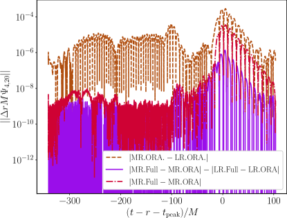
Restricting to the $\lambda=0.04m^{2}$ run for the order-by-order approach, we compare the difference in the amplitude of the waveform with the fully nonlinear solution to the numerical errors in the simulation. In Fig. 6, we show that, although the numerical error in the GW amplitude (dashed curve) is larger than the difference between the full and order-by-order solution (dash-dotted curve), the latter is larger than the difference between the full and order-by-order solutions at two resolutions. This arises because the dominant truncation error in our simulations does not depend strongly on the approach used or the coupling and thus partially cancels out when looking at the difference in the GW amplitude between the full and order-by-order solution using the same resolution.

Figure 6: We show the difference between the low and medium resolution (respectively labelled “LR" and “MR") of the amplitude of the gravitational waveform for non-spinning equal mass head-on collision with coupling of $\lambda=0.04m^{2}$ when solving system using the order-by-order approach (dashed brown curve). This is larger than the difference between the order-by-order and full solution at the medium resolution (red dash-dotted curve). However we also show the difference of the difference between the order-by-order and full GW amplitude at low and medium resolutions (solid purple curve). This provides evidence that the truncation error roughly cancels between the order by order and full runs.

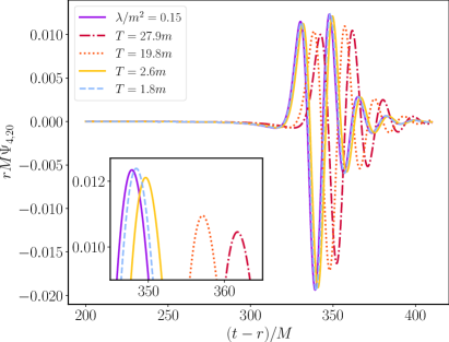
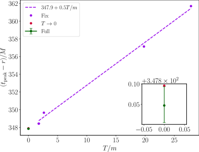
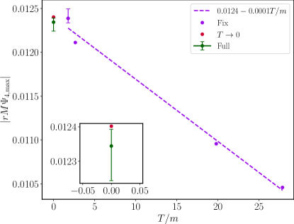
The waveforms obtained with the fixing-the-equations approach in Fig. 5 correspond to a single combination of fixing parameters. However, in a similar fashion to the single black hole case, one can evolve the system for a combination of parameters and extrapolate how the solution would behave as $T\rightarrow 0$. The left panel of Fig. 7 shows the gravitational waveforms when evolving the fixed system of equation assuming a coupling value of $\lambda=0.15m^{2}$ and using the following parameters for $t_{1}=\{0.4,0.3\}m$ while keeping $t_{2}=0.6m$ fixed, as well as letting $t_{1}=\{0.4,0.3\}m$ but keeping $t_{2}=2m$ fixed. In other words, the waveforms have a slowest decay rate of the solution to the simplified driver equation Eq. 41 of $T=\{1.8,2.6,19.8,27.9\}m$. Fitting the amplitude and the time at peak amplitude for a behavior $F=F_{0}+F_{1}T$, as shown Figs. 7 (right panel) and 8, we then extract what the values would be as $T\rightarrow 0$, obtaining a relative error of $\left(e_{t_{\rm peak}},e_{|\Psi_{4}|}\right)=(0.014,0.47)\%$.

Figure 7: Left: Gravitational waveforms for a coupling value of $\lambda=0.15m^{2}$ when solving the full system of equations (solid purple curve) and for four different combinations of fixing parameters with different decay rates $T$. Right: Time at which amplitude of waveforms peak and corresponding linear fit. The error bars represent estimates for the truncation error of full solution.

Figure 8: Peak amplitude of gravitational signal for a coupling value of $\lambda=0.15m^{2}$ when solving the fixed system of equations for four different combinations of fixing parameters with different decay rates $T$ and corresponding linear fit.

V.4 Quasi-circular inspirals of scalarized black holes

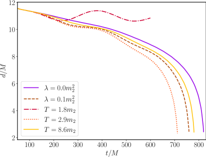
Finally, we consider the quasi-circular inspiral and merger of binary black holes. Here we focus on one GW150914-like system consisting of two non-spinning black holes with masses $m_{2}=0.4502M$ and $m_{1}=0.5497M$, giving a mass ratio of 1.22. We consider an initial separation of $9.8M$ corresponding to a system that undergoes $\sim 6$ orbital periods before merging in GR. We solve the full equations for coupling values of $\lambda/m_{2}^{2}=\{0,0.02,0.04,0.1\}$ and turn on the coupling at $t_{\rm start}=0$ but over a period of $200M$. For the largest coupling, we also solve the system using the fixing equations approach. We first tried fixing parameters that were found to give an accurate representation of the full solution when studying head-on collisions, $\{t_{1},t_{2}\}=\{0.75,0.9\}m_{2}$ but found that the black holes stopped inspiralling into each other shortly after the black holes acquired their individual charges (see Fig. 9). We attribute this behavior to insufficient numerical resolution to: (i) resolve the small values of $t_{1}$ and $t_{2}$ (which we recall, determine the final value of the scalar charge that the black holes acquire) and (ii) resolve the faster timescale in the decay defined by the fixed equations which is $\approx T/4$. Though the grid spacing on the finest adaptive mesh refinement level is $dx=0.016M$, for points at a distance of $\approx 10M$ from both black holes, the minimum linear grid spacing becomes comparable to $t_{1}/5$, so this scale is barely resolved. We thus instead consider two sets of fixing parameters with longer fixing timescales than the abovementioned run, namely $\{t_{1},t_{2}\}=\{2.2,2.3\}m_{2}$ and $\{t_{1},t_{2}\}=\{5.6,6.0\}m_{2}$. When performing the order-by-order approach, as explained in Sec. III.2, because of secular growth during the inspiral, we turn on the coupling of the theory as close to merger as possible, by first evolving the binary black hole system in GR, and then ramping on the source terms for the scalar field and metric perturbation at some later time $t_{\rm start}$.

Figure 9: (Left) Coordinate separation between black holes of quasi-circular inspiral of GW150914 like binary for a coupling of $\lambda=0.1m_{2}^{2}$ when solving the full equations and fixed system of equations with different fixing parameters. We also show the coordinate separation of the black holes in GR for comparison. (Right) Scalar charge measured at $100M$ as a function of look-back time for the solutions shown in left panel, with the exception of the fixed solution with slowest decay rate of $T=1.8m_{2}$.

We performed six simulations with different start times for turning on the EsGB correction in the order-by-order approach. In Fig. 10, we show the peak amplitude of the gravitational waveform as a function of inspiral length $L_{\rm insp}=t_{\rm peak}-t_{\rm start}-t_{\rm ramp}$. We find that the secular growth, as reflected in the peak amplitude, roughly behaves quadratically with the inspiral length (see Fig. 7 of Ref. Okounkova et al. (2020) and Fig. 4 of Ref. Okounkova (2020)). In a similar fashion to Refs. Okounkova et al. (2020); Okounkova (2020), which considered evolutions starting close to merger time in the hope of reducing the amount of secular growth, we choose the simulation with the closest start time to merger (unless stated otherwise), corresponding to an inspiral length of $\sim 140M$, as our representative waveform for the order by order approach. Of course, this is an artificial set-up which ignores the difference in dynamics prior to such time with respect to GR. We only adopt this approach here to compare with such works.

Figure 10: Peak amplitude of the EsGB correction to the gravitational waveform as a function of inspiral length for quasi-circular binary inspiral in the order-by-order approach.

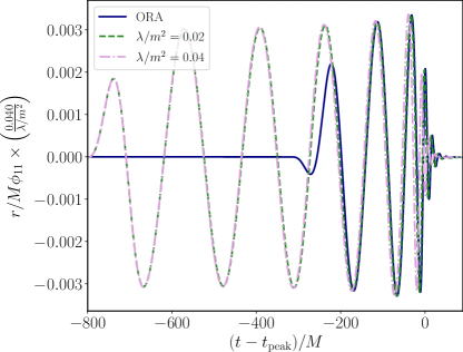
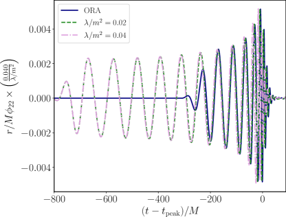
As mentioned in Sec. III.2.2, besides the secular breakdown, there is also an instantaneous regime of validity. For the waveform with inspiral length of $\sim 140M$, evaluating Eq. 19 gives $\lambda/m_{2}^{2}\lesssim 0.13C$ with the minimum occurring at merger, where the strong-field effects are the largest. In the left panel of Fig. 11, we compare the real part of the $\ell=m=2$ harmonic of the GW strain $h_{22}$ of our representative order-by-order waveform to the gravitational wave strain one obtains when solving the full system of equations for coupling values of $\lambda=\{0.02,0.04,0.1\}m_{2}^{2}$. We align the waveforms in time and phase at the peak of the complex amplitude of the waveform. In the right panel of Fig. 11, we again compare the real part of the $\ell=m=2$ harmonic of the GW strain one obtains when solving the full system to the order-by-order waveform for coupling values of $\lambda=\{0.02,0.04\}m_{2}^{2}$ (where we omitted 0.1 for clarity), but we consider order-by-order solution obtained when turning on the scalar field at $t_{\rm start}=0$ to illustrate the effect of a longer inspiral. We align the waveforms in time and phase at some fiducial frequency $\omega_{m}M=0.064$ early on in the inspiral. Note that the coupling values are already approaching the regime where estimates based on the size of the metric contribution [e.g. Eq. 19] suggest the perturbative scheme in the order-by-order approach may be breaking down; Though, on the other hand, we find that the deviations from GR for values below these values are very small, and hence not very useful to assess the validity of the order-by-order approach. To that end, we also show the waveform assuming GR for comparison. We find that both the order-by-order and full waveform have a phase shift relative to the GR solution, but the accumulation of secular effects in the waveform obtained from turning on scalar field at $t_{\rm start}=0$ leads to the EsGB waveform inspiraling slower than the GR waveform, which is in disagreement with the expectation that the EsGB waveform should inspiral faster due to the additional energy loss to the scalar field. We verify this statement by confirming that the order-by-order solution does inspiral faster than GR when using the representative waveform which has a shorter inspiral length as in left panel of Fig. 11. However, we find that even when using the shortest inspiral length possible, the order-by-order approach overestimates the amplitude shift and underestimates the dephasing relative to GR. This is consistent with the spurious increase in amplitude of oscillations we found in Appendix D when solving the anharmonic oscillator order by order over timescales that are sufficiently long to obtain noticeable dephasing.

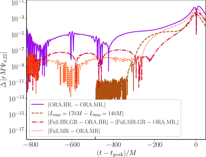
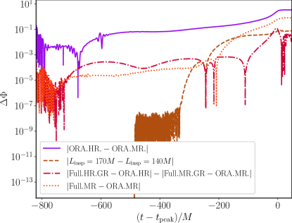
In Fig. 12, we quantify how the difference between the order-by-order and full solution for a coupling value of $\lambda=0.04m_{2}^{2}$ compares to the truncation error of our simulations. To do so, we split the $\ell=m=2$ harmonic of $\Psi_{4}$ into a real phase $\Phi$ and amplitude $|\Psi_{4,22}|$ so that $\Psi_{4,22}(r,t)=|\Psi_{4,22}|e^{-i\Phi(r,t)}$ and consider the differences in each quantity separately. Figure 12 shows that, just as for the head-on collision, the difference in amplitude $rM\Delta|\Psi_{4,22}|$ (left) and phase $\Delta\Phi$ (right) of the gravitational waveform between the high and medium resolutions of the order-by-order solution (solid curve) is larger than the difference between the full and order-by-order solution at medium resolution (dashed curve). However, because we use the same numerical resolution for carrying out the order-by-order and full solution and find that the dominant truncation error in our simulations does not depend strongly on the approach used or coupling, the truncation error will partially cancel out when calculating the difference in the phase and amplitude between the order-by-order and full solution using the same resolution. This is illustrated by the dash-dotted curve in Fig. 12, where we estimate the truncation error in the difference between the order-by-order and full solution by comparing the order-by-order and full solutions at two different resolutions (dash-dotted curve), finding it to be smaller than the difference obtained at the medium resolution. We also present the difference in amplitude and phase of waveforms when turning on the coupling at slightly different times which is smaller than the difference between the full and order-by-order solution. These findings imply that one can not take at face value bounds obtained on EsGB gravity with the order-by-order approach Okounkova (2020).

Figure 11: Gravitational wave radiation in the order-by-order approach and when solving the full equations for coupling values of $\lambda=\{0.02,0.04,0.1\}m_{2}^{2}$ as well as GR ($\lambda=0$). We show the real part of the $\ell=m=2$ spherical harmonic of the GW strain $h$. Left: The waveforms are aligned in phase and time at peak amplitude and the inspiral length of the ORA waveform is $\sim 140M$. Right: The waveforms are aligned in phase and time at a frequency of $\omega_{m}M=0.064$ and the inspiral length of the ORA waveform is $\sim 600M$. The $\lambda=0.1m_{2}^{2}$ case is not included for easier visualization of the better behaved solutions.

Figure 12: Difference between high and medium resolutions of the amplitude (left) and phase (right) of the gravitational waveform for the GW150914-like binary with coupling $\lambda=0.04m_{2}^{2}$ in the order-by-order approach (solid curve). We also show the difference in amplitude and phase when turning on the coupling at two different times in order-by-order approach (dashed curve), as well as the difference between solving the full equations and the order-by-order equations at medium resolution (dotted curve) and the difference between the full and order-by-order solutions at high and medium resolution (dash-dotted). This provides evidence that the truncation error cancels between the order-by-order and full runs.

Figure 13: Scalar waveforms as a function of retarded time measured from the time at which the gravitational waveform in GR peaks, rescaled by extraction radius $r=100M$ and scaling out the decoupling behavior for the full solutions shown in Fig. 11, as well as the order-by-order solution. We show the $\ell=m=2$ and $\ell=m=1$ spherical harmonic components.

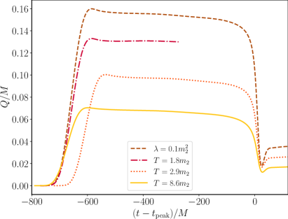
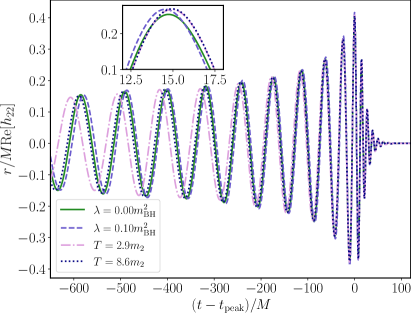
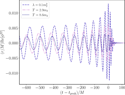
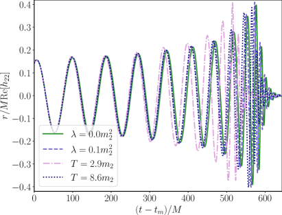
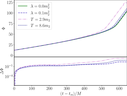
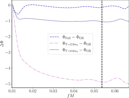
We finish this section by presenting the results of evolving the GW150914-like binary assuming a coupling of $\lambda=0.1m_{2}^{2}$, when solving the full and fixed system of equation. In Fig. 14, we show the gravitational (left) and scalar (right) waveforms aligned in time and phase at the peak of the amplitude of the gravitational waveforms. We show results for two sets of fixing parameters chosen to have longer timescales than the ones that gave us the most accurate results in the head-on collisions to ensure that all relevant timescales are properly resolved. As shown in the right panel of Fig. 9, we find that, in agreement with the results above, the smaller the slowest decay timescale is, the larger—and hence, the closer to the full solution—the scalar charge is, which in turn leads to a faster the inspiral (see, for instance, the phase of the GW in the right panel of Fig. 15). However, unlike for the head-on collisions, we find that, despite the scalar charge and scalar waveforms being noticeably smaller in amplitude than the full solution, the two fixed solutions merge earlier than the full solution. The careful reader will have noticed that from the trajectories of the black holes shown in Fig. 9 one would conclude that the fixing solution with the largest decaying timescale, namely $T=8.6m_{2}$, merges later than the full solution. However, after aligning the waveforms at merger, as in Fig. 14, or alternatively at some fiducial frequency, as in Fig. 15, we conclude that the fixing solution lags the full solution, although by a very little amount. The right panel of Fig. 15 shows the phase of each solution in the top panel, and the difference between the phase in GR and the full or fixed solution after alignment. This confirms the statement that the shorter the decay rate of the fixed solution, the faster the inspiral and the larger the error compared with the full solution, which is shown as a function of GW frequency in Fig. 16.

The reason for this requires further investigation. This is likely due to a lack of numerical resolution, but another possible cause is inconsistent initial data. It is possible that as we slowly turn on the scalar field, the fixed solution moves to a different orbit—e.g., a slightly more eccentric one—compared with the full solution. Another source of error for the inspiral case that is worth pointing out is that the initial velocities of the individual black holes in the inspiral case are roughly $3\times$ larger than in the head-on collisions where we set the initial velocities to the values corresponding to the binary being marginally bound at infinite separation. However, remember that the fixing parameters $\{t_{1},t_{2}\}$ determine the timescale over which the auxiliary fields are driven to their corresponding true value, and thus if the timescale over which the true solution changes decreases, then one would have to decrease the fixing parameters accordingly to keep the error in the fixed solution unchanged. We verified that the error in the amplitude and time of merger in the head-on collision for a fixed set of fixing parameters increases with the initial speed of the individual black holes. The study of all these effects is beyond the scope of this paper.

Figure 14: Gravitational (left) and scalar (right) waveforms for the GW150914-like binary of coupling $\lambda=0.1m_{2}^{2}$ when solving the full and fixed system of equations with two sets of fixing parameters. The GR waveform is shown for comparison. We align the waveform in phase and time at the peak of the amplitude of gravitational waveform.

Figure 15: Left: Gravitational waveforms for the GW150914-like binary with coupling $\lambda=0.1m_{2}^{2}$ when solving the full and fixed system of equations with two sets of fixing parameters. All the waveforms are aligned in time and phase at some fiducial frequency chosen to be $\omega_{m}M=0.065$. Right: The GW phase of the aligned waveforms $\Phi$. The bottom plot shows the phase difference between the EsGB and GR waveforms. Time is measured with respect to the time where the waveforms are aligned in frequency and phase.

Figure 16: Left: The dephasing compared to GR as a function of GW frequency $fM$ for the GW150914-like binary with coupling $\lambda=0.1m_{2}^{2}$ when solving the full and fixed system of equations. The dashed vertical line represents the frequency at which the waveform peaks in GR.

VI Discussion and Conclusion

In this work, we have performed the first systematic and fully self-consistent comparison of the three different numerical approaches commonly used in the literature to study extensions of GR in the strong-field, highly dynamical regime. The three approaches we compared are: (i) solving the full evolution equations, (ii) solving the equations order by order, and (iii) solving a fixed system of evolution equations. By leveraging our ability to solve the full equations of motions in a particular theory, we were able to quantify the errors introduced by secular effects in the order-by-order approach and by different prescriptions for the ad-hoc dynamical fields with finite damping timescales in the fixing-the-equations approach. We focused on shift-symmetric EsGB gravity as a benchmark, and considered the dynamical formation of scalar hair around non-spinning black holes in axisymmetry, head-on black hole collisions, and quasi-circular binary black hole mergers.

For single black hole spacetimes, we found that, for small enough couplings, the order-by-order approach accurately reproduces the formation of scalar hairy black hole solutions, but that nonlinear effects become important for couplings below the threshold for which perturbation theory breaks down. The fixing-the-equations approach, however, is able to track the scalarization of the black hole even at large couplings, provided we choose a good set of fixing parameters. We guided and justified our choices for a good combination of fixing parameters by analytically solving for a simpler fixing equation that retained most of the features of the full solution. This toy equation illustrated that the decaying solution is subject to two different timescales. We define good parameters as ones that will lead to both solutions decaying at roughly the same rate while avoiding oscillatory and singular behavior. Another requirement is that the decay rate of both solutions be smaller than all the relevant timescales in system under study. Of course, in a numerical implementation, care must be exercised to ensure that the resulting timescales are not too small as to become poorly resolved. However, even better solutions can be obtained through extrapolation to vanishing timescales over which the auxiliary fields are driven to their corresponding true value. Finally, for our particular choice of driver equation, making the fixing timescales sufficiently short was important to avoid spurious spatial dependence in the stationary solution. Of course, alternative driver choices could be devised, e.g., by adding a suitable contribution to source term or considering a different order of driver equation. However, these would introduce only mild effects as we see no significant energy cascade to the UV. Thus, differences introduced by the choice of driver are not essential, as argued in Refs. Geroch (1995); Cayuso et al. (2023) and we do not concern ourselves with other options for this work.

We next studied the head-on collision of an equal-mass binary black hole in axisymmetry, considering a range of coupling values. Our results were entirely consistent with the single black hole spacetimes. We found that the order-by-order approach does well at small couplings, but ceases to yield a good approximation even for couplings below which the perturbative approximation breaks down. The fixing approach, on the other hand, does well even for moderately large couplings provided the fixing parameters are chosen wisely. In the order-by-order approach, we found that the dominant source of error arises in the amplitude of the gravitational waveform, rather than the merger time.

We finished our study by considering the astrophysically relevant inspiral and merger of binary black holes without any continuous symmetries. Here, we focused on a single system with parameters similar to the GW150914 event. As expected, the order-by-order solution is subject to secular effects in the amplitude of the waveform. We found that these errors are small only when the coupling is small enough that the deviations from GR in the waveform—which occur primarily as a dephasing—are negligible. We conclude that one cannot use this approach in the way it has been implemented to place useful constraints on EsGB gravity. As this issue is generic, it will likely prevent one from obtaining faithful solutions using this approach in other beyond GR theories.

In this study, for computational expedience, we only applied the fixing-the-equations approach to a moderately large coupling quasicircular merger. We adopted approximate initial data and accounted for the scalarized solution by a transition to the corresponding coupling over an extended time frame. With this choice, employing fixing parameters with a short time for the damping parameters gave an unphysical behavior, which we believe is due to a lack of resolution for the timescales involved. With the same resolution, we evolved the system for two other sets of parameters with somewhat longer timescales, which gave better results, but we were unable to see a trend one could extrapolate. Based on the results for head-on collisions, we expect that one will be able to obtain accurate solutions in this approach using sufficiently short fixing timescales with sufficiently high resolution, though as a practical matter, the higher resolution requirements are an impediment. Constructing initial data and a different combination of fixing parameters may also help improve the accuracy of the solution. This observation was supported by additional studies of head-on collisions starting at increasingly larger speeds.

We note that recent work Lara et al. (2024) applied the fixing-the-equations approach to study spontaneous scalarization in EsGB gravity taking the decoupling limit (i.e. considering a test field) and proposed a new driver equation that improved the accuracy of their stationary solutions. Though it is unclear whether such choice was a consequence of implementing the approach under a dual-frame strategy.

The question remains whether one could modify the order-by-order approach in a way that would give useful results, e.g., by “renormalizing" in some way Gálvez Ghersi and Stein (2021). One option may be to renormalize the correction the GW signal, as opposed to working with the full spacetime solution. Given that the main source of error seems to be in the GW amplitude, while the main effect of the modified gravity (in EsGB, as well as other examples like the higher derivative gravity theory considered with the fixing-the-equations approach in Ref. Cayuso et al. (2023)) seems to be in the phase evolution, one could imagine devising a way to interpret the correction derived in the order-by-order approach as solely one to the frequency evolution.

We have only simulated the dynamics of one of the simplest EsGB gravity theories that gives scalar hairy black holes. Although we believe our comparison should also apply to other kinds of sGB couplings—and the general conclusions should be broadly applicable to modified gravity theories—it would be interesting to perform the comparison we did on coupling functions that allow for the effect of (de)scalarization, which will change the second order equations in the order-by-order approach, and also might affect the timescales we consider in the fixing-the-equations approach. Similarly including spin can significantly impact the dynamics of binaries. Finally, our results argue for applying the fixing-the-equations approach to other classes of theories which cannot be formulated in a well-posed manner. We note that in those theories, unlike the one studied here (at sufficiently small coupling), it may not be possible to make the fixing timescales arbitrarily small, and instead one may need to establish that there is a regime where these timescales are sufficiently small so that the results are insensitive to them, but not too small as to reintroduce the instabilities associated with ill-posedness.

VII Acknowledgments

We thank Miguel Bezares, Ramiro Cayuso, Guillermo Lara, Peter James Nee, Harald Pfeiffer, Justin Ripley, and Thomas Sotiriou for discussions. W.E. and L.L. acknowledge support from the Natural Sciences and Engineering Research Council of Canada through a Discovery Grant. L.L. also thanks financial support via the Carlo Fidani Rainer Weiss Chair at Perimeter Institute and CIFAR. W.E. is also supported by an Ontario Ministry of Colleges and Universities Early Researcher Award. This research was supported in part by Perimeter Institute for Theoretical Physics. Research at Perimeter Institute is supported in part by the Government of Canada through the Department of Innovation, Science and Economic Development and by the Province of Ontario through the Ministry of Colleges and Universities. This research was enabled in part by support provided by SciNet (www.scinethpc.ca) and the Digital Research Alliance of Canada (alliancecan.ca). Calculations were performed on the Symmetry cluster at Perimeter Institute, the Niagara cluster at the University of Toronto, and the Urania cluster at the Max Planck Institute for Gravitational Physics.

Appendix A Implementation of evolution equations for shift-symmetric EsGB gravity

Here we give some details on the numerical implementation of the order-by-order and fixing-the-equations approach in the numerical scheme we use to evolve the full EsGB equations. To do so, we first write down the MGH equations of motion in the form we numerically evolve, namely

$$\begin{pmatrix}\mathcal{A}_{ab}{}^{ef}&\mathcal{B}_{ab}\\ \mathcal{C}^{ef}&\mathcal{D}\end{pmatrix}\partial_{0}^{2}\begin{pmatrix}g_{ef}\\ \phi\end{pmatrix}=\begin{pmatrix}\mathcal{S}_{ab}^{(g)}\\ \mathcal{S}^{(\phi)}\end{pmatrix},$$ (28)

where the explicit forms of the components are derived in Appendix A of Ref. East and Ripley (2021a). We note that this includes constraint damping terms Gundlach et al. (2005) designed to damp away violations of the MGH constraint

$$C^{a}\equiv H^{a}-\tilde{g}^{bc}\nabla_{b}\nabla_{c}x^{a}=0.$$ (29)

In all three approaches, we set the constraint damping timescale to be $\sim M$. Using this hyperbolic system of equations, we directly evolve the 22 variables (after accounting for the symmetries of the metric components) $\{g_{ab},\partial_{t}g_{ab},\phi,\partial_{t}\phi\}$ through a method-of-lines algorithm.

The goal now is to rewrite the order-by-order Eqs. 8, 11 and 13a and fixed Eqs. 20, 21 and 23 system of equations in the same form as Eq. 28, such that we can re-use the already existing numerical scheme.

A.1 Order by order approach

Considering the order-by-order approach first, recall that to evolve the first order metric perturbation, we need to evolve three systems of equations simultaneously: one for the GR background $g^{(0)}_{ab}$ Eq. 8, one for the first order scalar field $\phi^{(1)}$ sourced by background curvature Eq. 11, and one for the metric perturbation $h^{(2)}_{ab}$ Eq. 13a sourced by background metric and $\phi^{(1)}$. Let us rewrite these equations in the same form as Eq. 28. We do this order by order. At zeroth order in $\epsilon$, we obtained Eq. 7a, i.e. a pure GR Einstein field equation. This is then equivalent to the system we solve for Eq. 28 provided we set all the terms introducing modifications from GR to zero,

$$\begin{pmatrix}\mathcal{A}_{ab}{}^{ef}&0\\ 0&\mathcal{D}\end{pmatrix}\partial_{0}^{2}\begin{pmatrix}g^{(0)}_{ef}\\ \phi^{(0)}\end{pmatrix}=\begin{pmatrix}\mathcal{S}_{ab}^{(g)}\\ \mathcal{S}^{(\phi)}\end{pmatrix},$$ (30)

all evaluated using $(g_{ab},\phi)=(g_{ab}^{(0)},\phi^{(0)})$ and setting $\lambda=0$. Since the scalar field equation has no source, we also take $\phi^{(0)}=0$ which simplifies the system even further. In fact we no longer have to solve the scalar field equation. We will use this to simultaneously solve for the background metric and first order scalar field.

At first order in $\epsilon$, we find that the equations of motion for the first order perturbation to the metric and scalar field are given by Eq. 11, i.e., the Einstein equations do not have a source term and the scalar field is sourced by the curvature of the background spacetime only. Rewriting this system in the form we are numerically implementing gives,

$$\begin{pmatrix}\mathcal{A}_{ab}{}^{ef}&0\\ 0&\mathcal{D}\end{pmatrix}\partial_{0}^{2}\begin{pmatrix}h^{(1)}_{ef}\\ \phi^{(1)}\end{pmatrix}=\begin{pmatrix}\mathcal{S}_{ab}^{(g)}\\ \mathcal{S}^{(\phi)}\end{pmatrix},$$ (31)

where all the functions involving the metric in the scalar sector are evaluated using the zeroth order GR solution $g^{(0)}$. The metric sector does not depend on the first order scalar field or in other words it is not sourced. This means that we can solve for both the zeroth order metric and first order scalar field by solving the system

$$\begin{pmatrix}\mathcal{A}_{ab}{}^{ef}&0\\ \mathcal{C}^{ef}&\mathcal{D}\end{pmatrix}\partial_{0}^{2}\begin{pmatrix}g^{(0)}_{ef}\\ \phi^{(1)}\end{pmatrix}=\begin{pmatrix}\mathcal{S}_{ab}^{(g)}\\ \mathcal{S}^{(\phi)}\end{pmatrix}.$$ (32)

Instead of solving for the second order perturbation directly, we choose to solve for the full metric, but making the perturbation sufficiently small that any $\mathcal{O}(\epsilon^{3})$ term can be neglected. The system we then solve for is,

$$\begin{pmatrix}\mathcal{A}_{ab}{}^{ef}&\mathcal{B}_{ab}\\ 0&1\end{pmatrix}\partial_{0}^{2}\begin{pmatrix}g_{ef}\\ \phi^{(1)}\end{pmatrix}=\begin{pmatrix}\mathcal{S}_{ab}^{(g)}\\ \partial_{0}^{2}\phi^{(1)}\end{pmatrix},$$ (33)

where

$$\mathcal{A}_{ab}{}^{ef}\equiv A_{ab}{}^{00ef},$$ (34a)

$$\mathcal{B}_{ab}\equiv B_{ab}{}^{00},$$ (34b)

$$\mathcal{S}_{ab}^{(g)}\equiv -2A_{ab}{}^{(0\alpha)ef}\partial_{0}\partial_{\alpha}g_{ef}-A_{ab}{}^{\alpha\beta ef}\partial_{\alpha}\partial_{\beta}g_{ef}$$ (34c)

$$-2B_{ab}{}^{(0\alpha)}\partial_{0}\partial_{\alpha}\phi-B_{ab}{}^{\alpha\beta}\partial_{\alpha}\partial_{\beta}\phi-F_{ab}^{(g)}$$

where $B_{ab}{}^{cd}$ is evaluated using the background metric as any contribution coming from using the full metric would give a fourth order correction. Moving to the $A_{ab}{}^{cdef}$ term, the two contributions are the following (see also Eqs. (A8) and (A23) in East and Ripley (2021a)),

$$A_{ab}{}^{cdef}= \delta_{a}^{e}\delta_{b}^{f}g^{cd}-\left(\delta_{a}^{f}\delta_{b}^{d}g^{ce}-\delta_{a}^{f}\hat{g}_{b}{}^{d}\tilde{g}^{ce}\right)-\left(\delta_{a}^{c}\delta_{b}^{f}g^{de}-\delta_{b}^{f}\hat{g}_{a}{}^{c}\tilde{g}^{de}\right)+\left(\delta_{a}^{c}\delta_{b}^{d}g^{ef}-\delta_{(a}^{d}\hat{g}^{c}_{b)}\tilde{g}^{ef}\right)$$

$$-\left(g^{ce}\hat{g}_{ab}+\hat{g}^{ce}g_{ab}-\frac{1}{2}g_{ab}g^{ce}\hat{g}\right)\tilde{g}^{df}+\frac{1}{2}\left(g^{cd}\hat{g}_{ab}+g_{ab}\hat{g}^{cd}-\frac{1}{2}g_{ab}g^{cd}\hat{g}\right)\tilde{g}^{ef}$$ (35)

and

$$A_{ab}{}^{cdef}= \lambda g^{jd}g^{ie}g^{gl}\Delta^{cf\gamma}_{ijgab}\left[\partial_{l}\partial_{\gamma}\phi-\Gamma^{m}_{l\gamma}\partial_{m}\phi\right].$$ (36)

The first one is the same as if one were to evolve GR in the MGH formulation, while the second one includes the terms arising from introducing modification to GR. We use the full metric for the first term, but again choose the perturbation to be small enough that any higher order terms are negligible. However, for the same reasons as for $B_{ab}{}^{cd}$, we evaluate the second term using the background metric and first order scalar field. Note that, since we are using the background metric in both $B_{ab}{}^{cd}$ and the non-GR contribution to $\mathcal{A}_{ab}{}^{ef}$, these terms can be included in the right-hand side of the equation such that one recovers the same principal part as in GR as required. Applying similar reasoning, one can also simplify some of the contributions to the source terms $F^{(g)}_{ab}$. We test our implementation of the order-by-order approach by verifying that the appropriate scaling relations Eqs. 16 and 17 are satisfied.

A.2 Fixing equations approach

Let us now consider the fixing-the-equations approach, outlined in Sec. III.3, and rewrite the fixed system of equations Eqs. 20, 21 and 23 in the same form as Eq. 28. To do so, we move all the EsGB contribution to the right-hand side of Eq. 28 where the source terms are,

$$\begin{pmatrix}\mathcal{A}_{ab}{}^{{(\rm GR)}ef}&0\\ 0&\mathcal{D}\end{pmatrix}\partial_{0}^{2}\begin{pmatrix}g_{ef}\\ \phi\end{pmatrix}=\begin{pmatrix}\mathcal{S}_{ab}^{{(\rm GR)}(g)}+\mathcal{S}_{ab}^{{\rm(GB)}(g)}-\mathcal{B}_{ab}\partial_{0}^{2}\phi-\mathcal{A}_{ab}{}^{{(\rm GB)}ef}\partial_{0}^{2}g_{ef}\\ \mathcal{S}^{{\rm(GR)}(\phi)}+\mathcal{S}^{{\rm(GB)}(\phi)}-\mathcal{C}^{ef}\partial_{0}^{2}g_{ef}\end{pmatrix}.$$ (37)

Note that, by doing so, we have recovered the same principal part as in GR. Note that we also split the purely GR and additional EsGB contributions in the source terms. Introducing the source terms $\mathbf{S}=\left(\tilde{S}^{(g)}_{ab},\tilde{S}^{(\phi)}\right)$, which include all contributions from EsGB, one has

$$\begin{pmatrix}\mathcal{A}_{ab}{}^{{(\rm GR)}ef}&0\\ 0&\mathcal{D}\end{pmatrix}\partial_{0}^{2}\begin{pmatrix}g_{ef}\\ \phi\end{pmatrix}=\begin{pmatrix}\mathcal{S}_{ab}^{{(\rm GR)}(g)}\\ \mathcal{S}^{{\rm(GR)}(\phi)}\end{pmatrix}-\begin{pmatrix}\tilde{S}^{(g)}_{ab}\\ \tilde{S}^{(\phi)}\end{pmatrix}.$$ (38)

Introducing eleven massive fields $\mathbf{P}=\left(\Pi^{(\phi)},\Pi^{(g)}_{ab}\right)$, we write the system as,

$$\begin{pmatrix}\mathcal{A}_{ab}{}^{{(\rm GR)}ef}&0\\ 0&\mathcal{D}\end{pmatrix}\partial_{0}^{2}\begin{pmatrix}g_{ef}\\ \phi\end{pmatrix}=\begin{pmatrix}\mathcal{S}_{ab}^{{(\rm GR)}(g)}\\ \mathcal{S}^{{\rm(GR)}(\phi)}\end{pmatrix}-\begin{pmatrix}\Pi^{(g)}_{ab}\\ \Pi^{(\phi)}\end{pmatrix}.$$ (39)

When $\Pi=\tilde{S}$, the equations are ‘unfixed.’ To fix the equations, we choose the driver equation Eq. 23,

$$\sigma g^{ab}\partial_{a}\partial_{b}\mathbf{P}= \partial_{0}\mathbf{P}+\kappa\left(\mathbf{P}-\mathbf{S}\right).$$ (40)

Note that the source terms depend on second derivatives in time of the metric and scalar field $\mathbf{S}=\mathbf{S}\left[\ldots\partial_{0}^{2}g,\partial_{0}^{2}\phi\ldots\right]$. We compute those by applying order reduction, i.e. we substitute the zeroth order solutions to the second time derivatives, obtained by solving for Eq. 38 with $\mathbf{S}=0$. This implies that the solutions to the fixed system Eqs. 20, 21 and 23 are valid to first order in the coupling of the theory.

Finally, in order to justify and guide our choices for the fixing parameters $\{\sigma,\kappa\}$, we analytically solve for a simpler fixing equation (where we set any spatial dependence to zero), albeit with most of the features of the true fixed equation,

$$\sigma\frac{d^{2}P}{dt^{2}}+\frac{dP}{dt}+\kappa(P-1)=0.$$ (41)

The general solution to this equation, subject to $P(0)=dP/dt(0)=0$, is

$$P(t)=-e^{a_{+}t}\frac{(-\sqrt{-4\kappa\sigma+1}+4\kappa\sigma-1)}{2(4\kappa\sigma-1)}$$ (42)

$$-e^{a_{-}t}\frac{(\sqrt{-4\kappa\sigma+1}+4\kappa\sigma-1)}{2(4\kappa\sigma-1)}+1,$$

where

$$a_{+}=\frac{-1+\sqrt{1-4\kappa\sigma}}{2\sigma}\,\,\,,\,\,\,a_{-}=-\frac{1+\sqrt{1-4\kappa\sigma}}{2\sigma}.$$ (43)

The solutions to this system will decay, but depending on the values chosen for the fixing parameters, the solutions might undergo an oscillatory decay. Large oscillations will lead to stages where the system overshoots the original one, a feature that we consider it best to avoid. To keep both solutions decaying at roughly the same rate, and the frequency of oscillations small, one could choose $4\kappa\sigma\simeq 1$. In that case, the decay rate is $T\approx 2\sigma$, though care should be exercised to avoid singular behavior indicated by the solution, Eq. (42). The timescale should also be taken to be smaller than the smallest relevant scales in the problem being studied, in order to approach the original system; however, if the timescale $T$ is made too short, it may lead to stiff behavior in the numerical evolution, requiring higher resolution. Finally we note that, depending on the driver equation adopted, a small $\sigma$ is desirable to avoid spurious spatial dependence.

Appendix B Numerical convergence and consistency tests

Here we present convergence results and consistency tests for the implementation of the order-by-order and fixing-the-equations approach in the modified generalized harmonic code East and Ripley (2021a) that we use.

In the left panel of Fig. 17, we show the integrated MGH constraint violation $|C_{a}|$ as a function of coordinate time for a single black hole spacetime with $\lambda=0.1M^{2}$ (dashed curves) as well as GR (solid curves) and several resolutions, demonstrating that this quantity is converging to zero with third-order, as expected. Here, the lowest resolution has 6 levels of mesh refinement with a refinement ratio of $2:1$, and has a grid spacing of $dx\sim 0.024M$ on the finest level. The medium and high resolutions are $1.5$ and $2\times$ as high, respectively. The medium resolution is the default resolution for the results presented in this work. The transient growth at $\sim 50M$ is due to the slow ramp on of the scalar field. Similarly, in the right panel of Fig. 17, we show the integrated constraint violation for the equal-mass non-spinning head-on collision initially separated by $75M$ and with $\lambda=0.1m^{2}$. Here the lowest resolution has 7 levels of mesh refinement and a grid spacing of $dx\sim 0.008M$ on the finest mesh refinement. The medium and high resolution have, respectively, $4/3$ and $2\times$ the resolution of lowest resolution.

Figure 17: Integrated norm of the constraint violation $C_{a}$ as a function of coordinate time (in units of the total mass) for the scalarization of a single black hole spacetime with a coupling value of $\lambda=0.1M^{2}$ (left and dashed curves) and for an equal-mass head-on collision with $\lambda=0.1M^{2}$ (right) at three resolutions. The medium and high resolutions have $1.5$ and $2\times$ the resolution of the low resolution simulation. The solid lines in the left panel are the corresponding constraint violations in GR.

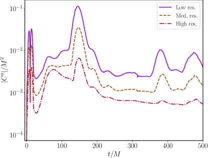
In Fig. 18, we test our numerical implementation of the order-by-order approach in our MGH code by comparing the maximum value of the scalar field and the correction to the $tt$ component of the metric for two different couplings, after scaling out the dependence on coupling using the results of Sec. III.2.1. We find that the difference between the scaled out quantities computed with two different coupling values is much smaller than the truncation error of solutions. This provides evidence that we correctly implemented the order-by-order approach. Similarly, in Fig. 19, we show that in the order-by-order approach the gravitational waveform scales quadratically with the coupling both for the head-on collision and quasi-circular inspiral of equal-mass non-spinning black holes.

Figure 18: Maximum value of scalar field and second-order correction to the $tt$ component of the metric for the scalarization of single black hole computed for two couplings at the default resolution (Med. res.) and after scaling out the dependence on $\lambda$. We also show the corresponding values for the low and high resolution runs.

Figure 19: Left: Second-order correction in gravitational waveform from the head-on collisions of equal-mass, non-spinning black holes for two different couplings and three different resolutions after scaling out the quadratic dependence on $\lambda$. We also show the correction at medium resolution when using a coupling of twice the canonical value and find that the difference is much smaller than the truncation error. Right: Gravitational waveform for GW150914-like binary in GR and EsGB assuming a coupling of $\lambda=0.02m_{2}^{2}$. We compare the full solution to the order-by-order solution computed for two couplings and assuming a quadratic dependence with the coupling. The fact that the two order-by-order solutions overlap provides evidence we correctly implemented the order-by-order approach.

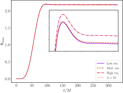
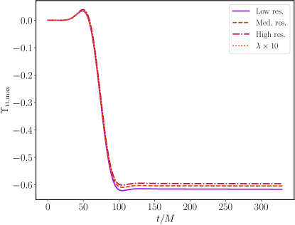
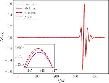
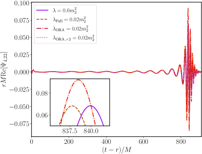
Appendix C Fixing equations and constraints

Here we argue that constraints are preserved by the fixed equations. First, recall that constraint damping in the generalized harmonic formulation is achieved by ensuring the effective evolution of the coordinate conditions is damped away (see Ref. Gundlach et al. (2005)). Such a behavior is enforced by adding a suitable contribution to Einstein equations that: (i) is proportional to the constraints, and (ii) is such that, upon taking the divergence and using the Bianchi identity, the constraints are seen to obey a homogeneous damped wave equation. As a result, violations of the constraints are driven towards zero.

In the case of beyond GR theories, extra contributions appear in the equations of motion in addition to the Einstein tensor. An analogous constraint damping strategy can be adopted in such cases (for an explicit discussion in the case of EsGB, see Ref. East and Ripley (2021a)), where one uses explicitly that the extra contributions should have zero divergence.

When fixing the equations, such an identity is not explicitly enforced. The resulting induced evolution equations for the constraint violation contains an additional source from the divergence of such tensor which must be shown to suitably approach zero in the adopted fixing-the-equations approach. We next argue this is the case.

The modified gravity theory in a suitable formulation is governed by

$$G^{ab}+S^{ab}+M^{ab} =Q^{ab},$$ (44)

where the beyond GR contributions are split into $S^{ab}$—containing contributions with second order derivatives—and $M^{ab}$—which contains the remaining terms, and $Q^{ab}$ is the constraint function that vanishes when the constraints are satisfied (for example, $F^{ab}$ in Eq. (21)). Furthermore, the divergence of $Q^{ab}$ gives rise to a damped evolution equation for the constraints, to converge to the left hand side, which is zero as $\nabla_{a}S^{ab}=-\nabla_{a}M^{ab}$. That is

$$\nabla_{a}\left(G^{ab}+S^{ab}+M^{ab}\right)=0=\nabla_{a}Q^{ab},$$ (45)

so the constraints are conserved. The fixed equations replace $S^{ab}$ by ${\Pi^{(g)}}_{ab}$ and provide an equation of motion for this tensor to approach $S^{ab}$:

$$G^{ab}+\Pi^{ab}+M^{ab} =Q^{ab}.$$ (46)

Notice that $\nabla_{a}M^{ab}={\Pi^{\phi}}\nabla_{b}\phi$ by definition and, due to the fixed equation introduced for its dynamics, it approaches $-2\lambda{\cal G}\nabla_{b}\phi$ . We next argue that the fixing equation enforces that $\nabla_{a}\Pi^{ab}$ approaches $\nabla_{a}S^{ab}$ in a controlled manner.

Starting with the equation of motion for $\Pi_{ab}$:

$$\nabla_{c}\nabla^{c}\Pi^{ab} =\frac{1}{\sigma}n^{c}\nabla_{c}\Pi^{ab}+\frac{\kappa}{\sigma}\left(\Pi^{ab}-S^{ab}\right),$$ (47)

where, for simplicity, we adopted a slightly different form of the equation than the one used explicitly in this work to aid in the presentation. Next, we take the covariant derivative

$$\nabla_{a}\nabla_{c}\nabla^{c}\Pi^{ab} -\frac{1}{\sigma}\nabla_{a}\left(n^{c}\nabla_{c}\Pi^{ab}\right)$$

$$-\frac{\kappa}{\sigma}\left(\nabla_{a}\Pi^{ab}-\nabla_{a}S^{ab}\right)=0.$$ (48)

Using the fact that $R_{ab}\simeq\mathcal{O}\left(\lambda\right)$, the first term, to order $\mathcal{O}\left(\lambda^{2}\right)$, gives

$$\nabla_{a}\nabla_{c}\nabla^{c}\Pi^{ab} =\nabla_{c}\nabla_{a}\nabla^{c}\Pi^{ab}-R_{ace}{}^{b}\nabla^{c}\Pi^{ae}$$

$$=\Box\left(\nabla_{a}\Pi^{ab}\right)-R_{ace}{}^{b}\nabla^{c}\Pi^{ae}-\nabla^{c}\left(R_{ace}{}^{b}\Pi^{ae}\right).$$ (49)

Proceeding analogously, to the same order, the second term gives

$$\nabla_{a}\left(n^{c}\nabla_{c}\Pi^{ab}\right) =\left(\nabla_{a}n^{c}\right)\nabla_{c}\Pi^{ab}+n^{c}\nabla_{a}\nabla_{c}\Pi^{ab}$$

$$=\left(\nabla_{a}n^{c}\right)\nabla_{c}\Pi^{ab}+n^{c}\nabla_{c}\nabla_{a}\Pi^{ab}-n^{c}R_{ace}{}^{b}\Pi^{ae}.$$ (50)

Combining it all together we have

$$0= \Box\left(\nabla_{a}\Pi^{ab}\right)-\frac{1}{\sigma}n^{c}\nabla_{c}\left(\nabla_{a}\Pi^{ab}\right)$$

$$- \frac{\kappa}{\sigma}\left(\nabla_{a}\Pi^{ab}-\nabla_{a}S^{ab}-\frac{1}{\kappa}n^{c}R_{ace}{}^{b}\Pi^{ae}\right)$$

$$- R_{ace}{}^{b}\nabla^{c}\Pi^{ae}-\nabla^{c}\left(R_{ace}{}^{b}\Pi^{ae}\right)$$

$$- \frac{1}{\sigma}\left(\nabla_{a}n^{c}\right)\nabla_{c}\Pi^{ab}.$$ (51)

The first two lines drive $\nabla_{a}\Pi^{ab}$ to $\nabla_{a}S^{ab}+(1/\kappa)\,n^{c}R_{ace}^{b}\Pi^{ae}$. The first term is precisely what cancels the contribution from $\nabla_{a}M^{ab}$, and the second one is not only subleading with respect to curvature, but also can be made smaller by a judicious choice of $\kappa$. To examine the role of the other contributions, we can use the cyclic symmetries of the Riemann tensor and $\Pi^{ab}=\Pi^{(ab)}$. The third line simplifies, because

$$\Pi^{ae}\nabla^{c}R_{ace}{}^{b} =-\Pi^{ae}\nabla^{c}\left(R_{cea}{}^{b}+R_{eac}{}^{b}\right)$$ (52)

$$=-\Pi^{ae}\nabla^{c}R_{cea}{}^{b}$$ (53)

$$=-\Pi^{ae}g^{bd}\nabla_{c}R^{c}{}_{ead}$$ (54)

$$=\Pi^{ae}g^{bd}\left(\nabla_{a}R^{c}{}_{edc}+\nabla_{d}R^{c}{}_{eca}\right)\sim\mathcal{O}\left(\lambda^{2}\right).$$ (55)

So we then have

$$R_{ace}{}^{b}\nabla^{c}\Pi^{ae} =\nabla^{c}\left(R_{ace}{}^{b}\Pi^{ae}\right)+\mathcal{O}\left(\lambda^{2}\right).$$ (56)

The third line and the last term from the second line give

$$2\nabla^{c}F_{c}{}^{b}-\frac{1}{\sigma}n^{c}F_{c}{}^{b},$$ (57)

$$F_{c}{}^{b}:=R_{ace}{}^{b}\Pi^{ae}.$$ (58)

This contribution is not only proportional to curvature terms, but also has an extra order of derivatives, which should be subleading in the valid EFT regime. Thus, $\nabla_{a}\Pi^{ab}$ converges to $\simeq\nabla_{a}S^{ab}+(1/\kappa)\,n^{c}R_{ace}^{b}\Pi^{ae}$. The last term can be reduced by the choice of $\kappa$. As a consequence, the divergence of Eq. (46) gives rise to controlled dynamics for the constraints, approximating the behavior from the original system, as expected.

In our studies, we have confirmed this behavior and, unless the timescale $T$ employed is much larger than the scale of the black holes considered, the constraints remain under control and the solutions show a convergent behavior throughout the evolutions. We show the behavior of the constraint violation with increasing numerical resolution in Fig. 20, and when increasing $\kappa$ in Fig. 21. The constraint violation is found to decrease with one or the other, depending on which contribution dominates at a given time.

Figure 20: Integrated norm of the constraint violation $C_{a}$ as a function of coordinate time (in units of the total mass) for the scalarization of a single black hole spacetime with a coupling value of $\lambda=0.04M^{2}$ (left) and for an equal-mass head-on collision with $\lambda=0.04m^{2}$ (right) at three resolutions when solving the fixed system of equations. The damping parameters for the single black hole are $\{\sigma,\kappa\}=\{0.2M,0.5/M\}$ so that $T=1.8M$, and similarly for the head-on collision, where $M$ is now mass of each individual black hole. The medium and high resolutions have $1.5$ and $2\times$ the resolution of the low resolution simulation.

Figure 21: Integrated norm of the constraint violation $C_{a}$ as a function of coordinate time (in units of the total mass) for the same equal-mass head-on collision with $\lambda=0.04m^{2}$ shown in the right panel of Fig. 20 when varying $t_{1}$ but keeping $t_{2}$ fixed (left), or varying $t_{2}$ but keeping $t_{1}$ fixed (right). As expected, the constraints decrease with increasing $\kappa$.

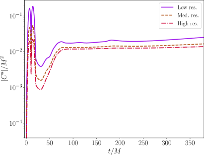
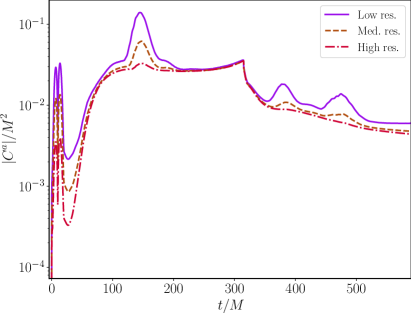
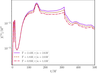
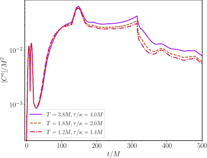
Appendix D Secular errors in the order-by-order approach: a toy model

As a toy model to illustrate how secular errors appear in the order-by-order approach, let us consider the anharmonic oscillator

$$\frac{d^{2}x}{dt^{2}}+\left(\frac{2\pi}{T_{0}}\right)^{2}\left(x^{2}+\epsilon x^{3}\right)=0,$$ (59)

where we will consider $\epsilon$ to be a smaller parameter, and choose initial conditions with

$$x(t=0)=1,\ \frac{dx}{dt}(t=0)=0.$$ (60)

For $\epsilon>0$, the system will oscillate with shorter period compared to $\epsilon=0$ (where the period is $T_{0}$), but will have the same amplitude of oscillation. This is similar to binary black hole mergers in EsGB, where we find non-zero coupling causes the binary to inspiral faster compared to GR, and hence the frequency of the GW signal increases, but we find that the amplitude of the GW signal at fixed frequency is not significantly affected.

Solving Eq. 59 to linear order in $\epsilon$ in the order-by-order approach with the specified initial conditions, we obtain

$$x(t)= \cos(\omega_{0}t)$$ (61)

$$+\frac{\epsilon}{32}\left[\cos(3\omega_{0}t)-\cos(\omega_{0}t)-12\omega_{0}t\sin(\omega_{0}t)\right]$$

where $\omega_{0}=2\pi/T_{0}$. From this, we can immediately see that this solution will exhibit secular growth on timescales of the order of $T_{0}/\epsilon$. This is illustrated in Fig. 22, where we compare the order-by-order solution to the full solution taking $\epsilon=0.01$. With this value, the anharmonic oscillator becomes out of phase with the $\epsilon=0$ case by $\sim 1$ radian after $50T_{0}$. As shown in Fig. 22, the order-by-order approach captures the decrease in the period of oscillation initially, but over time, exhibits a secular increase in the period towards its unperturbed value.

This approximation also introduces an increase in the amplitude of oscillation, which at early times grows like $t^{2}$. By the time the effect of the $\epsilon$ term has led to a noticeable dephasing, the spurious increase in amplitude and period have also become significant. This simple model captures the features that we also find when considering binary black hole mergers in EsGB. In particular, whenever the modified gravity contribution causes a noticeable dephasing in the GWs, the ORA approach also gives a significant spurious increase in the amplitude of the GW signal.

Figure 22: A comparison of the solution to the anharmonic oscillator system [Eq. (61) with $\epsilon=0.01$] using the ORA approach (solid black curves) to the full solution (dashed blues curves). Left: The time evolution of the anharmonic oscillator compared to the harmonic oscillator (dotted red curve). The inset shows that after 50 oscillations, the anharmonic oscillator is noticeably out-of-phase compared to the harmonic ($\epsilon=0$) oscillator, and the ORA approximation has a spurious increase in amplitude. Right: The increase in amplitude (top) and period (bottom) of oscillator in the ORA solution. In the full solution, these quantities are constant.

Appendix E Fixing a potentially elliptic second order model

Consider the following equation

$$\partial_{t}^{2}\phi=\partial_{x}^{2}\phi+a\partial_{x}^{2}\phi\,,$$ (62)

for some value of $a\in\mathbb{R}$. If $a<-1$, this defines an elliptic second order equation for $\phi$; otherwise, the problem is hyperbolic. Unless the condition $a>-1$ is satisfied, an attempt treat the equation as normal hyperbolic evolution equation would fail. Consider instead the following fixed version,

$$\partial_{t}^{2}\phi = \partial_{x}^{2}\phi+a\Pi\ ,$$

$$\sigma\partial_{t}^{2}\Pi = \sigma\partial_{x}^{2}\Pi-\partial_{t}\Pi-\kappa(\Pi-\partial_{x}^{2}\phi)\ ,$$ (63)

which forces the variable $\Pi$ to approach $\partial_{x}^{2}\phi$ on a timescale $\simeq\kappa^{-1}$, and recover the behavior of the original equation for long wavelengths, while also forcing the system to be hyperbolic. A straightforward Fourier-mode analysis, i.e., assuming $\{\phi,\Pi\}=\{\phi,\Pi\}_{0}e^{st}e^{ikx}$, reveals the fixed system has, for low wavenumbers, four distinct solutions behaving as

$$s_{\pm} = \pm i(\sqrt{1+a})k+\frac{a}{2\kappa}k^{2}\ ,$$ (64)

$$s_{1,2} = -\frac{1}{2\sigma}\pm\frac{\sqrt{1-4\kappa\sigma}}{2\sigma}+\left(\pm\frac{2(1-a)\kappa\sigma+a}{2\kappa\sqrt{1-4\kappa\sigma}}-\frac{a}{2\kappa}\right)k^{2}\,.$$

Thus, it has two modes coinciding with the behavior expected in the original problem, and two extra ones which are damped away. For high wavenumbers, instead, one has two solutions with dual roots,

$$s=\pm ik\,,$$ (65)

which corresponds to plane wave solutions propagating with speed unity. This model highlights some features that are particularly relevant to EsGB gravity: If the hyperbolic condition is violated, the fixed system controls the high frequency behavior of the solution, but still retains the low frequency dispersion relation expected for the hyperbolic ($s=\pm\sqrt{1+a}ik$) or elliptic $s=\pm\sqrt{|1+a|}k$) cases.

References

- Will (2014) C. M. Will, Living Rev. Rel. 17, 4 (2014), arXiv:1403.7377 [gr-qc] .
- Clifton et al. (2012) T. Clifton, P. G. Ferreira, A. Padilla, and C. Skordis, Phys. Rept. 513, 1 (2012), arXiv:1106.2476 [astro-ph.CO] .
- Lee et al. (2020) J. G. Lee, E. G. Adelberger, T. S. Cook, S. M. Fleischer, and B. R. Heckel, Phys. Rev. Lett. 124, 101101 (2020), arXiv:2002.11761 [hep-ex] .
- Kapner et al. (2007) D. J. Kapner, T. S. Cook, E. G. Adelberger, J. H. Gundlach, B. R. Heckel, C. D. Hoyle, and H. E. Swanson, Phys. Rev. Lett. 98, 021101 (2007), arXiv:hep-ph/0611184 .
- Abuter et al. (2020) R. Abuter et al. (GRAVITY), Astron. Astrophys. 636, L5 (2020), arXiv:2004.07187 [astro-ph.GA] .
- Kramer et al. (2021) M. Kramer et al., Phys. Rev. X 11, 041050 (2021), arXiv:2112.06795 [astro-ph.HE] .
- Akiyama et al. (2019) K. Akiyama et al. (Event Horizon Telescope), Astrophys. J. Lett. 875, L5 (2019), arXiv:1906.11242 [astro-ph.GA] .
- Akiyama et al. (2022) K. Akiyama et al. (Event Horizon Telescope), Astrophys. J. Lett. 930, L17 (2022), arXiv:2311.09484 [astro-ph.HE] .
- Völkel et al. (2021) S. H. Völkel, E. Barausse, N. Franchini, and A. E. Broderick, Class. Quant. Grav. 38, 21LT01 (2021), arXiv:2011.06812 [gr-qc] .
- Psaltis et al. (2020) D. Psaltis et al. (Event Horizon Telescope), Phys. Rev. Lett. 125, 141104 (2020), arXiv:2010.01055 [gr-qc] .
- Kocherlakota et al. (2021) P. Kocherlakota et al. (Event Horizon Telescope), Phys. Rev. D 103, 104047 (2021), arXiv:2105.09343 [gr-qc] .
- Abbott et al. (2016a) B. P. Abbott et al. (LIGO Scientific, Virgo), Phys. Rev. Lett. 116, 221101 (2016a), [Erratum: Phys.Rev.Lett. 121, 129902 (2018)], arXiv:1602.03841 [gr-qc] .
- Yunes et al. (2016) N. Yunes, K. Yagi, and F. Pretorius, Phys. Rev. D 94, 084002 (2016), arXiv:1603.08955 [gr-qc] .
- Baker et al. (2017) T. Baker, E. Bellini, P. G. Ferreira, M. Lagos, J. Noller, and I. Sawicki, Phys. Rev. Lett. 119, 251301 (2017), arXiv:1710.06394 [astro-ph.CO] .
- Isi et al. (2019) M. Isi, M. Giesler, W. M. Farr, M. A. Scheel, and S. A. Teukolsky, Phys. Rev. Lett. 123, 111102 (2019), arXiv:1905.00869 [gr-qc] .
- Isi et al. (2020) M. Isi, W. M. Farr, M. Giesler, M. A. Scheel, and S. A. Teukolsky, (2020), arXiv:2012.04486 [gr-qc] .
- Okounkova et al. (2022) M. Okounkova, W. M. Farr, M. Isi, and L. C. Stein, Phys. Rev. D 106, 044067 (2022), arXiv:2101.11153 [gr-qc] .
- Abbott et al. (2019a) B. P. Abbott et al. (LIGO Scientific, Virgo), Phys. Rev. Lett. 123, 011102 (2019a), arXiv:1811.00364 [gr-qc] .
- Abbott et al. (2019b) B. P. Abbott et al. (LIGO Scientific, Virgo), Phys. Rev. D 100, 104036 (2019b), arXiv:1903.04467 [gr-qc] .
- Abbott et al. (2020) R. Abbott et al. (LIGO Scientific, Virgo), (2020), arXiv:2010.14529 [gr-qc] .
- Abbott et al. (2021a) R. Abbott et al. (LIGO Scientific, VIRGO, KAGRA), (2021a), arXiv:2112.06861 [gr-qc] .
- Aasi et al. (2015) J. Aasi et al. (LIGO Scientific), Class. Quant. Grav. 32, 074001 (2015), arXiv:1411.4547 [gr-qc] .
- Acernese et al. (2015) F. Acernese et al. (VIRGO), Class. Quant. Grav. 32, 024001 (2015), arXiv:1408.3978 [gr-qc] .
- Somiya (2012) K. Somiya (KAGRA), Class. Quant. Grav. 29, 124007 (2012), arXiv:1111.7185 [gr-qc] .
- Aso et al. (2013) Y. Aso, Y. Michimura, K. Somiya, M. Ando, O. Miyakawa, T. Sekiguchi, D. Tatsumi, and H. Yamamoto (KAGRA), Phys. Rev. D 88, 043007 (2013), arXiv:1306.6747 [gr-qc] .
- Abbott et al. (2021b) R. Abbott et al. (LIGO Scientific, Virgo), Phys. Rev. D 103, 122002 (2021b), arXiv:2010.14529 [gr-qc] .
- Ghosh (2022) A. Ghosh (LIGO Scientific–Virgo–Kagra), in 56th Rencontres de Moriond on Gravitation (2022) arXiv:2204.00662 [gr-qc] .
- Yunes and Siemens (2013) N. Yunes and X. Siemens, Living Rev. Rel. 16, 9 (2013), arXiv:1304.3473 [gr-qc] .
- Berti et al. (2015) E. Berti et al., Class. Quant. Grav. 32, 243001 (2015), arXiv:1501.07274 [gr-qc] .
- Berti et al. (2018a) E. Berti, K. Yagi, and N. Yunes, Gen. Rel. Grav. 50, 46 (2018a), arXiv:1801.03208 [gr-qc] .
- Berti et al. (2018b) E. Berti, K. Yagi, H. Yang, and N. Yunes, Gen. Rel. Grav. 50, 49 (2018b), arXiv:1801.03587 [gr-qc] .
- Damour and Esposito-Farese (1993) T. Damour and G. Esposito-Farese, Phys. Rev. Lett. 70, 2220 (1993).
- Barausse et al. (2013) E. Barausse, C. Palenzuela, M. Ponce, and L. Lehner, Phys. Rev. D 87, 081506 (2013), arXiv:1212.5053 [gr-qc] .
- Shibata et al. (2014) M. Shibata, K. Taniguchi, H. Okawa, and A. Buonanno, Phys. Rev. D 89, 084005 (2014), arXiv:1310.0627 [gr-qc] .
- Garfinkle et al. (1991) D. Garfinkle, G. T. Horowitz, and A. Strominger, Phys. Rev. D 43, 3140 (1991), [Erratum: Phys.Rev.D 45, 3888 (1992)].
- Hirschmann et al. (2018) E. W. Hirschmann, L. Lehner, S. L. Liebling, and C. Palenzuela, Phys. Rev. D97, 064032 (2018), arXiv:1706.09875 [gr-qc] .
- de Rham et al. (2023) C. de Rham, J. Kożuszek, A. J. Tolley, and T. Wiseman, Phys. Rev. D 108, 084052 (2023), arXiv:2302.04876 [hep-th] .
- Noakes (1983) D. R. Noakes, J. Math. Phys. 24, 1846 (1983).
- Held and Lim (2021) A. Held and H. Lim, Phys. Rev. D 104, 084075 (2021), arXiv:2104.04010 [gr-qc] .
- Held and Lim (2023) A. Held and H. Lim, (2023), arXiv:2306.04725 [gr-qc] .
- East and Siemonsen (2023) W. E. East and N. Siemonsen, Phys. Rev. D 108, 124048 (2023), arXiv:2309.05096 [gr-qc] .
- Papallo and Reall (2017) G. Papallo and H. S. Reall, Phys. Rev. D 96, 044019 (2017), arXiv:1705.04370 [gr-qc] .
- Kovacs and Reall (2020a) A. D. Kovacs and H. S. Reall, Phys. Rev. Lett. 124, 221101 (2020a), arXiv:2003.04327 [gr-qc] .
- Kovacs and Reall (2020b) A. D. Kovacs and H. S. Reall, Phys. Rev. D 101, 124003 (2020b), arXiv:2003.08398 [gr-qc] .
- Ripley and Pretorius (2019a) J. L. Ripley and F. Pretorius, Phys. Rev. D 99, 084014 (2019a), arXiv:1902.01468 [gr-qc] .
- Bernard et al. (2019) L. Bernard, L. Lehner, and R. Luna, Phys. Rev. D 100, 024011 (2019), arXiv:1904.12866 [gr-qc] .
- East and Ripley (2021a) W. E. East and J. L. Ripley, Phys. Rev. D 103, 044040 (2021a), arXiv:2011.03547 [gr-qc] .
- East and Ripley (2021b) W. E. East and J. L. Ripley, Phys. Rev. Lett. 127, 101102 (2021b), arXiv:2105.08571 [gr-qc] .
- East and Pretorius (2022) W. E. East and F. Pretorius, (2022), arXiv:2208.09488 [gr-qc] .
- Corman et al. (2023) M. Corman, J. L. Ripley, and W. E. East, Phys. Rev. D 107, 024014 (2023), arXiv:2210.09235 [gr-qc] .
- Aresté Saló et al. (2022) L. Aresté Saló, K. Clough, and P. Figueras, Phys. Rev. Lett. 129, 261104 (2022), arXiv:2208.14470 [gr-qc] .
- Aresté Saló et al. (2023) L. Aresté Saló, K. Clough, and P. Figueras, Phys. Rev. D 108, 084018 (2023), arXiv:2306.14966 [gr-qc] .
- Figueras and França (2022) P. Figueras and T. França, Phys. Rev. D 105, 124004 (2022), arXiv:2112.15529 [gr-qc] .
- Bezares et al. (2022) M. Bezares, R. Aguilera-Miret, L. ter Haar, M. Crisostomi, C. Palenzuela, and E. Barausse, Phys. Rev. Lett. 128, 091103 (2022), arXiv:2107.05648 [gr-qc] .
- Alexander and Yunes (2009) S. Alexander and N. Yunes, Phys. Rept. 480, 1 (2009), arXiv:0907.2562 [hep-th] .
- Okounkova et al. (2017) M. Okounkova, L. C. Stein, M. A. Scheel, and D. A. Hemberger, Phys. Rev. D 96, 044020 (2017), arXiv:1705.07924 [gr-qc] .
- Okounkova et al. (2019a) M. Okounkova, L. C. Stein, M. A. Scheel, and S. A. Teukolsky, Phys. Rev. D 100, 104026 (2019a), arXiv:1906.08789 [gr-qc] .
- Okounkova et al. (2020) M. Okounkova, L. C. Stein, J. Moxon, M. A. Scheel, and S. A. Teukolsky, Phys. Rev. D 101, 104016 (2020), arXiv:1911.02588 [gr-qc] .
- Okounkova (2020) M. Okounkova, Phys. Rev. D 102, 084046 (2020), arXiv:2001.03571 [gr-qc] .
- Endlich et al. (2017) S. Endlich, V. Gorbenko, J. Huang, and L. Senatore, JHEP 09, 122 (2017), arXiv:1704.01590 [gr-qc] .
- Cayuso et al. (2017) J. Cayuso, N. Ortiz, and L. Lehner, Phys. Rev. D 96, 084043 (2017), arXiv:1706.07421 [gr-qc] .
- Cayuso and Lehner (2020) R. Cayuso and L. Lehner, Phys. Rev. D 102, 084008 (2020), arXiv:2005.13720 [gr-qc] .
- Lara et al. (2022) G. Lara, M. Bezares, and E. Barausse, Phys. Rev. D 105, 064058 (2022), arXiv:2112.09186 [gr-qc] .
- Franchini et al. (2022) N. Franchini, M. Bezares, E. Barausse, and L. Lehner, (2022), arXiv:2206.00014 [gr-qc] .
- Allwright and Lehner (2019) G. Allwright and L. Lehner, Class. Quant. Grav. 36, 084001 (2019), arXiv:1808.07897 [gr-qc] .
- Kanti et al. (1998) P. Kanti, N. Mavromatos, J. Rizos, K. Tamvakis, and E. Winstanley, Phys. Rev. D 57, 6255 (1998), arXiv:hep-th/9703192 .
- Yunes and Stein (2011) N. Yunes and L. C. Stein, Phys. Rev. D 83, 104002 (2011), arXiv:1101.2921 [gr-qc] .
- Sotiriou and Zhou (2014a) T. P. Sotiriou and S.-Y. Zhou, Phys. Rev. Lett. 112, 251102 (2014a), arXiv:1312.3622 [gr-qc] .
- Sotiriou and Zhou (2014b) T. P. Sotiriou and S.-Y. Zhou, Phys. Rev. D 90, 124063 (2014b), arXiv:1408.1698 [gr-qc] .
- Yagi et al. (2012) K. Yagi, L. C. Stein, N. Yunes, and T. Tanaka, Phys. Rev. D 85, 064022 (2012), [Erratum: Phys.Rev.D 93, 029902 (2016)], arXiv:1110.5950 [gr-qc] .
- Sennett et al. (2016) N. Sennett, S. Marsat, and A. Buonanno, Phys. Rev. D 94, 084003 (2016), arXiv:1607.01420 [gr-qc] .
- Shiralilou et al. (2021a) B. Shiralilou, T. Hinderer, S. Nissanke, N. Ortiz, and H. Witek, Phys. Rev. D 103, L121503 (2021a), arXiv:2012.09162 [gr-qc] .
- Shiralilou et al. (2021b) B. Shiralilou, T. Hinderer, S. Nissanke, N. Ortiz, and H. Witek, (2021b), arXiv:2105.13972 [gr-qc] .
- van Gemeren et al. (2023) I. van Gemeren, B. Shiralilou, and T. Hinderer, Phys. Rev. D 108, 024026 (2023), arXiv:2302.08480 [gr-qc] .
- Julié et al. (2023) F.-L. Julié, V. Baibhav, E. Berti, and A. Buonanno, Phys. Rev. D 107, 104044 (2023), arXiv:2212.13802 [gr-qc] .
- Julié (2023) F.-L. Julié, (2023), arXiv:2312.16764 [gr-qc] .
- Ripley (2022) J. L. Ripley, (2022), arXiv:2207.13074 [gr-qc] .
- Witek et al. (2019) H. Witek, L. Gualtieri, P. Pani, and T. P. Sotiriou, Phys. Rev. D 99, 064035 (2019), arXiv:1810.05177 [gr-qc] .
- Silva et al. (2021) H. O. Silva, H. Witek, M. Elley, and N. Yunes, Phys. Rev. Lett. 127, 031101 (2021), arXiv:2012.10436 [gr-qc] .
- Elley et al. (2022) M. Elley, H. O. Silva, H. Witek, and N. Yunes, Phys. Rev. D 106, 044018 (2022), arXiv:2205.06240 [gr-qc] .
- Weinberg (2008) S. Weinberg, Phys. Rev. D 77, 123541 (2008), arXiv:0804.4291 [hep-th] .
- Abbott and et.al. (2019) B. P. Abbott and et.al. (The LIGO Scientific Collaboration and the Virgo Collaboration), Phys. Rev. D 100, 104036 (2019).
- Agathos et al. (2014) M. Agathos, W. Del Pozzo, T. G. F. Li, C. Van Den Broeck, J. Veitch, and S. Vitale, Phys. Rev. D 89, 082001 (2014).
- Mehta et al. (2023) A. K. Mehta, A. Buonanno, R. Cotesta, A. Ghosh, N. Sennett, and J. Steinhoff, Phys. Rev. D 107, 044020 (2023).
- Dideron et al. (2023) G. Dideron, S. Mukherjee, and L. Lehner, Phys. Rev. D 107, 104023 (2023), arXiv:2209.14321 [gr-qc] .
- Ripley and Pretorius (2020) J. L. Ripley and F. Pretorius, Phys. Rev. D 101, 044015 (2020), arXiv:1911.11027 [gr-qc] .
- Yagi et al. (2016) K. Yagi, L. C. Stein, and N. Yunes, Phys. Rev. D 93, 024010 (2016), arXiv:1510.02152 [gr-qc] .
- Lyu et al. (2022) Z. Lyu, N. Jiang, and K. Yagi, Phys. Rev. D 105, 064001 (2022), arXiv:2201.02543 [gr-qc] .
- Okounkova et al. (2019b) M. Okounkova, M. A. Scheel, and S. A. Teukolsky, Class. Quant. Grav. 36, 054001 (2019b), arXiv:1810.05306 [gr-qc] .
- Okounkova et al. (2019c) M. Okounkova, M. A. Scheel, and S. A. Teukolsky, Phys. Rev. D 99, 044019 (2019c), arXiv:1811.10713 [gr-qc] .
- Okounkova (2019) M. Okounkova, Phys. Rev. D 100, 124054 (2019), arXiv:1909.12251 [gr-qc] .
- Okounkova et al. (2023) M. Okounkova, M. Isi, K. Chatziioannou, and W. M. Farr, Phys. Rev. D 107, 024046 (2023), arXiv:2208.02805 [gr-qc] .
- Logan (2013) J. Logan, Applied Mathematics (Wiley, 2013).
- Israel and Stewart (1976) W. Israel and J. M. Stewart, Physics Letters A 58, 213 (1976).
- Israel (1976) W. Israel, Annals Phys. 100, 310 (1976).
- Geroch (1995) R. Geroch, Journal of Mathematical Physics 36, 4226 (1995), https://pubs.aip.org/aip/jmp/article-pdf/36/8/4226/19174133/4226_1_online.pdf .
- Bezares et al. (2021) M. Bezares, L. ter Haar, M. Crisostomi, E. Barausse, and C. Palenzuela, Phys. Rev. D 104, 044022 (2021), arXiv:2105.13992 [gr-qc] .
- Cayuso et al. (2023) R. Cayuso, P. Figueras, T. França, and L. Lehner, Phys. Rev. Lett. 131, 111403 (2023), arXiv:2303.07246 [gr-qc] .
- Ripley and Pretorius (2019b) J. L. Ripley and F. Pretorius, Class. Quant. Grav. 36, 134001 (2019b), arXiv:1903.07543 [gr-qc] .
- East et al. (2012a) W. E. East, F. Pretorius, and B. C. Stephens, Phys. Rev. D 85, 124010 (2012a), arXiv:1112.3094 [gr-qc] .
- Lindblom and Szilagyi (2009) L. Lindblom and B. Szilagyi, Phys. Rev. D80, 084019 (2009), arXiv:0904.4873 [gr-qc] .
- Choptuik and Pretorius (2010) M. W. Choptuik and F. Pretorius, Phys. Rev. Lett. 104, 111101 (2010), arXiv:0908.1780 [gr-qc] .
- Brady et al. (2023) S. E. Brady, L. Aresté Saló, K. Clough, P. Figueras, and A. P. S., Phys. Rev. D 108, 104022 (2023), arXiv:2308.16791 [gr-qc] .
- East et al. (2012b) W. E. East, F. M. Ramazanoglu, and F. Pretorius, Phys. Rev. D 86, 104053 (2012b), arXiv:1208.3473 [gr-qc] .
- Ansorg et al. (2004) M. Ansorg, B. Bruegmann, and W. Tichy, Phys. Rev. D 70, 064011 (2004), arXiv:gr-qc/0404056 .
- Paschalidis et al. (2013) V. Paschalidis, Z. B. Etienne, R. Gold, and S. L. Shapiro, (2013), arXiv:1304.0457 [gr-qc] .
- (107) “Standalone TwoPunctures,” https://github.com/JLRipley314/Standalone-TwoPunctures-C-Cpp.
- Abbott et al. (2016b) B. P. Abbott et al. (LIGO Scientific, Virgo), Phys. Rev. Lett. 116, 241102 (2016b), arXiv:1602.03840 [gr-qc] .
- Abbott et al. (2016c) B. P. Abbott et al. (LIGO Scientific, Virgo), Phys. Rev. Lett. 116, 061102 (2016c), arXiv:1602.03837 [gr-qc] .
- Lehner and Moreschi (2007) L. Lehner and O. M. Moreschi, Phys. Rev. D 76, 124040 (2007), arXiv:0706.1319 [gr-qc] .
- Christodoulou (1970) D. Christodoulou, Phys. Rev. Lett. 25, 1596 (1970).
- Reisswig and Pollney (2011) C. Reisswig and D. Pollney, Class. Quant. Grav. 28, 195015 (2011), arXiv:1006.1632 [gr-qc] .
- Lara et al. (2024) G. Lara, H. P. Pfeiffer, N. A. Wittek, N. L. Vu, K. C. Nelli, A. Carpenter, G. Lovelace, M. A. Scheel, and W. Throwe, (2024), arXiv:2403.08705 [gr-qc] .
- Gálvez Ghersi and Stein (2021) J. T. Gálvez Ghersi and L. C. Stein, Phys. Rev. E 104, 034219 (2021), arXiv:2106.08410 [hep-th] .
- Gundlach et al. (2005) C. Gundlach, G. Calabrese, I. Hinder, and J. M. Martín-García, Classical and Quantum Gravity 22, 3767–3773 (2005).