Uniform $\mathcal{H}$-matrix Compression with Applications to Boundary Integral Equations

Abstract

Boundary integral equation formulations of elliptic partial differential equations lead to dense system matrices when discretized, yet they are data-sparse. Using the $\mathcal{H}$-matrix format, this sparsity is exploited to achieve $\mathcal{O}(N\log N)$ complexity for storage and multiplication by a vector. This is achieved purely algebraically, based on low-rank approximations of subblocks, and hence the format is also applicable to a wider range of problems. The $\mathcal{H}^{2}$-matrix format improves the complexity to $\mathcal{O}(N)$ by introducing a recursive structure onto subblocks on multiple levels. However, in practice this comes with a large proportionality constant, making the $\mathcal{H}^{2}$-matrix format advantageous mostly for large problems. In this paper we investigate the usefulness of a matrix format that lies in between these two: Uniform $\mathcal{H}$-matrices. An algebraic compression algorithm is introduced to transform a regular $\mathcal{H}$-matrix into a uniform $\mathcal{H}$-matrix, which maintains the asymptotic complexity. Using examples of the BEM formulation of the Helmholtz equation, we show that this scheme lowers the storage requirement and execution time of the matrix-vector product without significantly impacting the construction time.

1 Introduction

Solving linear systems of $N$ equations amounts to operating on $N\times N$-matrices. When using a dense $N\times N$-matrix directly, the storage requirements scale as $\mathcal{O}(N^{2})$, becoming prohibitively large if the problem size increases. In certain settings, such as finite element methods applied to partial differential equations (PDEs), the system matrix is naturally sparse in that only $\mathcal{O}(N)$ matrix entries are non-zero. In other applications, matrices arise that are not sparse in the usual sense but may still allow a data-sparse approximation. Examples are discretizations of integral equations or the solution operator – i.e. the inverse of the system matrix after discretization – of elliptic PDEs. The data-sparse hierarchical matrices ($\mathcal{H}$-matrices) are applicable in both these cases [16, 2, 11].

The hierarchical matrix framework, first introduced in [28], allows for storage of and operations with matrices in $\mathcal{O}(N\log N)$ complexity. This is achieved by splitting the matrix in appropriate submatrices of which the majority can be approximately represented by low-rank matrices. The approximation is constructed algebraically from a subset of entries of the matrix, using so-called Adaptive Cross Approximation (ACA) and similar techniques. Thus, the scheme is independent of the underlying problem and applicable in situations beyond PDEs and integral equations.

For integral operators of the form

$$(\mathcal{A}u)(\mathbf{x})=\int_{\Omega}{g(\mathbf{x},\mathbf{y})u(\mathbf{y})ds_{\mathbf{y}}}, \Omega\subseteq\mathbb{R}^{d}$$

similar techniques exist based on analytical expansions of the kernel function $g$. Originally, the Fast Multipole Method (FMM) [38, 27, 26] and the panel clustering method [31, 39] used explicit expansions of $g$ which are kernel-specific. This drawback is removed in kernel-independent variants [15, 41, 22, 34] but the utilized general expansions can become less efficient. This is demonstrated by comparing spherical harmonics with polynomials in three dimensions. The former uses $k=\mathcal{O}(\log^{2}\epsilon)$ terms in its expansions for a precision of $\epsilon$, while the latter requires $k=\mathcal{O}(\log^{3}\epsilon)$.

Improvement on the $\mathcal{H}$-matrix format have been developed in the form of $\mathcal{H}^{2}$-matrices [30], which employ a multilevel structure onto the low-rank factorizations of the subblocks. This hierarchical storage structure can improve the complexity to $\mathcal{O}(N)$. Yet, to enable construction in linear time, most $\mathcal{H}^{2}$-matrix frameworks fall back to analytic tools. To retain the generality of the algebraic approach, they utilize polynomial approximations [19] which often overestimate the rank of the blocks. For this reason, $\mathcal{H}^{2}$-matrices only become practically advantageous for very large problems. To alleviate this problem, schemes have been developed to recompress $\mathcal{H}^{2}$-matrices [30, 17, 7, 10]. This can even be performed during construction, such that the original uncompressed $\mathcal{H}^{2}$-matrix is never fully stored in memory. The technique has also been extended to directional $\mathcal{H}$-matrices ($\mathcal{DH}$-matrices) [12, 13, 18].

In the spirit of these recompression techniques, we investigate the compression of $\mathcal{H}$-matrices into the uniform $\mathcal{H}$-matrix format, which lies halfway between the $\mathcal{H}$- and $\mathcal{H}^{2}$-matrix formats. Uniform $\mathcal{H}$-matrices retain the $\mathcal{O}(N\log N)$ complexity of regular $\mathcal{H}$-matrices, but with an improved proportionality constant. This means that a constant compression factor is achieved with a relatively small implementation effort, owing to the simplicity of uniform $\mathcal{H}$-matrices (compared to the more involved $\mathcal{H}^{2}$-matrix format). While not asymptotically optimal, uniform $\mathcal{H}$-matrices retain the appeal of regular $\mathcal{H}$-matrices in that they are much easier to use. As we shall show, the format also enables a simple parallellization of the matrix-vector product. Interestingly, our numerical results indicate that the compression factor of memory usage leads to a similar improvement of the timings of the matrix-vector product.

Since its original introduction together with the regular $\mathcal{H}$-matrix [28], the uniform $\mathcal{H}$-matrix format has been explored very little. In [4], a recompression technique based on Chebyshev polynomials is proposed that leads to uniform $\mathcal{H}$-matrices, but reduction in memory usage is only achieved when doing considerable reassembly during the matrix-vector product. Apart from this reference, uniform $\mathcal{H}$-matrices are introduced as an intermediate step towards $\mathcal{H}^{2}$-matrices [30, 14], but do not seem to have been an object of study in their own right. With the above-mentioned advantages in mind, in this paper we aim to illustrate that any application using $\mathcal{H}$-matrices may, with little effort, benefit from using uniform $\mathcal{H}$-matrices instead.

During the writing of this paper, it has come to our attention that similar (unpublished) work on uniform $\mathcal{H}$-matrices has been independently done by R. Kriemann. An implementation is available in the codebase libHLR and preliminary results indicate, as we describe in more detail in this paper, that the uniform $\mathcal{H}$-matrix format results in memory reduction. Recent work by Kriemann on memory reduction includes mixed-precision compression of structured matrix formats in [33].

The structure of the paper is as follows. Section 2 introduces regular and uniform $\mathcal{H}$-matrices in the general setting. In Section 3, the Boundary Element Method and the $\mathcal{H}$-matrices that arise from this application are discussed. Then, Section 4 proposes a technique to compress regular $\mathcal{H}$-matrices into uniform $\mathcal{H}$-matrices. Error analysis on this compression is provided in Section 5. Lastly, Section 6 presents numerical results on the compression scheme applied to matrices that originate from a boundary integral formulation of the Helmholtz equation and Section 7 gives a brief conclusion.

2 Hierarchical matrices

This section gives a brief introduction to regular (§2.1) and uniform (§2.2) $\mathcal{H}$-matrices. For a more in-depth exposition on the subject, we refer to the books by Bebendorf [1] and Hackbusch [29], which have served as the basis for this section.

2.1 Regular $\mathcal{H}$-matrices

The $\mathcal{H}$-matrix format is based on partioning a matrix $A\in\mathbb{C}^{I\times J}$ into submatrices such that each submatrix can be approximately represented by a matrix of low rank. As $\mathcal{H}$-matrix methods aim to approximate the matrix in quasilinear complexity, i.e. quasilinear in the dimensions $|I|$ and $|J|$ of the matrix, subdividing the set ${I\times J}$ directly is infeasible. Typically, the partition is induced by hierarchical subdivisions of the row and column indices $I$ and $J$ separately.

A hierarchy of subsets of an index set $I$ is defined using a cluster tree $\mathcal{T}_{I}$.

Definition 1 (cluster tree).

A cluster tree $\mathcal{T}_{I}$ for an index set $I$ is a tree with $I$ as its root, that employs a subdivion strategy $s:\mathcal{P}(I)\to\mathcal{P}(I)\times\dots\times\mathcal{P}(I)$ at each non-leaf node such that

• the children of a node form a partition of their parent,

  $$\tau=\bigcup_{\tau^{\prime}\in s(\tau)}\tau^{\prime}\quad\text{for all}\leavevmode\nobreak\ \tau\in\mathcal{T}_{I}\leavevmode\nobreak\ \text{with}\leavevmode\nobreak\ s(\tau)\neq\emptyset;\leavevmode\nobreak\ \text{and}$$

• children of the same parent are disjoint,

  $$\tau_{1}\neq\tau_{2}\Rightarrow\tau_{1}\cap\tau_{2}=\emptyset\quad\text{for all}\leavevmode\nobreak\ \tau\in\mathcal{T}_{I},\leavevmode\nobreak\ \tau_{1},\tau_{2}\in s(\tau).$$

Nodes of a cluster tree are called clusters. The leaves of a cluster tree are denoted by $\mathcal{L}(\mathcal{T}_{I})$.

To each cluster $\tau\in\mathcal{T}_{I}$, we can ascribe its level as the distance (in number of applications of $s$) to the root $I$ by $\mathrm{level}(\tau)$. Each level

$$\mathcal{T}_{I}^{(\ell)}:=\{\tau\in\mathcal{T}_{I}:\mathrm{level}(\tau)=\ell\}$$

of $\mathcal{T}_{I}$ is a collection of disjoint subsets of $I$. The total number of levels in a cluster tree is called its depth and is denoted by $L(\mathcal{T}_{I}):=\max_{\tau\in\mathcal{T}_{I}}\mathrm{level}(\tau)+1$.

A pair of clusters $(\tau,\sigma),\leavevmode\nobreak\ \tau\subset I,\sigma\subset J$, defines a subset ${\tau\times\sigma}$ of ${I\times J}$ and thus also a submatrix of $A\in\mathbb{C}^{I\times J}$. From two cluster trees $\mathcal{T}_{I}$ and $\mathcal{T}_{J}$, a block cluster tree can be constructed.

Definition 2 (block cluster tree).

Given cluster trees $\mathcal{T}_{I}$ and $\mathcal{T}_{J}$ for index sets $I$ and $J$ respectively, a block cluster tree $\mathcal{T}_{I\times J}$ for ${I\times J}$ is a cluster tree of ${I\times J}$ where

• each node in $\mathcal{T}_{I\times J}$ originates from a pair of cluster nodes in $\mathcal{T}_{I}$ and $\mathcal{T}_{J}$,

  $$\forall b\in\mathcal{T}_{I\times J},\leavevmode\nobreak\ \exists\tau\in\mathcal{T}_{I},\sigma\in\mathcal{T}_{J}\leavevmode\nobreak\ \text{s.t.}\leavevmode\nobreak\ b={\tau\times\sigma};\leavevmode\nobreak\ \text{and}$$

• for each non-leaf node $b={\tau\times\sigma}\in\mathcal{T}_{I\times J}$, either $s(b)=s(\tau)\times s(\sigma)$, $s(b)=\{\tau\}\times s(\sigma)$ or $s(b)=s(\tau)\times\{\sigma\}$ holds.

Nodes of a block cluster tree are called blocks. Given $b={\tau\times\sigma}\in\mathcal{T}_{I\times J}$, $\tau\in\mathcal{T}_{I}$ and $\sigma\in\mathcal{T}_{J}$ are referred to as its row and column cluster respectively.

A block cluster tree $\mathcal{T}_{I\times J}$ induces a partition of ${I\times J}$ through its leaves

$$\mathcal{L}(\mathcal{T}_{I\times J}):=\{b\in\mathcal{T}_{I\times J}:s(b)=\emptyset\}.$$

This partition corresponds to a subdivision of matrix $A\in\mathbb{C}^{I\times J}$ into submatrices which we denote by ${A}_{|{\tau\times\sigma}}\in\mathbb{C}^{\tau\times\sigma}$ for all ${\tau\times\sigma}\in\mathcal{L}(\mathcal{T}_{I\times J})$.

Constructing an $\mathcal{H}$-matrix approximation of $A$ is achieved by finding an approximate low-rank factorization for each submatrix ${A}_{|{\tau\times\sigma}}$. However, in general, not all these submatrices will have approximate low rank. Therefore, the leaves are divided into an admissible part $\mathcal{L}^{+}(\mathcal{T}_{I\times J})\subset\mathcal{L}(\mathcal{T}_{I\times J})$ and inadmissible (or dense) part $\mathcal{L}^{-}(\mathcal{T}_{I\times J}):=\mathcal{L}(\mathcal{T}_{I\times J})\setminus\mathcal{L}^{+}(\mathcal{T}_{I\times J})$.

The partitions $P_{I\times J}:=\mathcal{L}(\mathcal{T}_{I\times J})$, $P^{+}_{I\times J}:=\mathcal{L}^{+}(\mathcal{T}_{I\times J})$ and $P^{-}_{I\times J}:=\mathcal{L}^{-}(\mathcal{T}_{I\times J})$ allow us to state the definition of a hierarchical matrix.

Definition 3 (hierarchical matrix).

A hierarchical matrix ($\mathcal{H}$-matrix) is a matrix $A\in\mathbb{C}^{I\times J}$ together with a partition $P_{I\times J}$ of ${I\times J}$ with admissible subset $P^{+}_{I\times J}\subset P_{I\times J}$, such that for all blocks ${\tau\times\sigma}\in P^{+}_{I\times J}$,

$$\exists X\in\mathbb{C}^{\tau\times k},Y\in\mathbb{C}^{\sigma\times k}:\quad{A}_{|{\tau\times\sigma}}=XY^{*}$$

where $k:=k({\tau\times\sigma})$ is variable across submatrices.

Given a matrix $A\in\mathbb{C}^{I\times J}$, we denote its $\mathcal{H}$-matrix approximation by $A^{\mathcal{H}}$. In an implementation, to represent an $\mathcal{H}$-matrix one needs to store the low-rank submatrices as well as the dense ones,

$$\{(X_{b},Y_{b})\}_{b\in P^{+}_{I\times J}}\leavevmode\nobreak\ \text{and}\leavevmode\nobreak\ \{{A}_{|b}\}_{b\in P^{-}_{I\times J}},$$

where we have added subscripts to $X$ and $Y$ to distinguish between factorizations. The amount of storage this requires is characterized by the defining partitions and the rank distribution ${(k_{b})}_{b\in P^{+}_{I\times J}}$ of the factorizations.

2.2 Uniform $\mathcal{H}$-matrices

In regular $\mathcal{H}$-matrices, as defined above, the low-rank factorizations of the admissible blocks are independent of each other. This setup is flexible but does not allow sharing of information across blocks. Storage requirements can be reduced by introducing a basis associated with each cluster, and to store a low-rank submatrix in terms of the bases of its row and column clusters.

The only clusters to consider are those in $\mathcal{T}_{I}$ or $\mathcal{T}_{J}$ that actually occur in admissible leaves of $\mathcal{T}_{I\times J}$. They are respectively

$$\mathcal{L}_{I}^{\prime}:=\mathcal{L}_{I}^{\prime}(\mathcal{T}_{I\times J})=\{\tau\in\mathcal{T}_{I}:\exists\sigma\in\mathcal{T}_{J}\leavevmode\nobreak\ \leavevmode\nobreak\ \text{s.t.\ }\leavevmode\nobreak\ {\tau\times\sigma}\in\mathcal{L}^{+}(\mathcal{T}_{I\times J})\},$$ (1)

$$\mathcal{L}_{J}^{\prime}:=\mathcal{L}_{J}^{\prime}(\mathcal{T}_{I\times J})=\{\sigma\in\mathcal{T}_{J}:\exists\tau\in\mathcal{T}_{I}\leavevmode\nobreak\ \leavevmode\nobreak\ \text{s.t.\ }\leavevmode\nobreak\ {\tau\times\sigma}\in\mathcal{L}^{+}(\mathcal{T}_{I\times J})\}.$$

The cluster bases are two families of matrices for these sets of clusters:

$$\mathcal{U}:=\{U_{\tau}\in\mathbb{C}^{\tau\times\ell_{\tau}}\}_{\tau\in\mathcal{L}_{I}^{\prime}}\leavevmode\nobreak\ \text{and}\leavevmode\nobreak\ \mathcal{V}:=\{V_{\sigma}\in\mathbb{C}^{\sigma\times\ell_{\sigma}}\}_{\sigma\in\mathcal{L}_{J}^{\prime}},$$

in which $(\ell_{\tau})_{\tau\in\mathcal{L}_{I}^{\prime}}$ and $(\ell_{\sigma})_{\sigma\in\mathcal{L}_{J}^{\prime}}$ are their corresponding rank distributions. First established in [28], the concept of row and column cluster bases introduces a new type of hierarchical matrix.

Definition 4 (uniform hierarchical matrix).

A uniform hierarchical matrix ($\mathcal{UH}$-matrix) is a matrix $A\in\mathbb{C}^{I\times J}$ together with a partition $P_{I\times J}$ of ${I\times J}$ with admissible subset $P^{+}_{I\times J}\subset P_{I\times J}$, and with row and column cluster bases $\mathcal{U}$ and $\mathcal{V}$, such that for all blocks $b={\tau\times\sigma}\in P^{+}_{I\times J}$:

$$\exists S_{b}\in\mathbb{C}^{\ell_{\tau}\times\ell_{\sigma}}:\quad{A}_{|b}=U_{\tau}S_{b}V_{\sigma}^{*}.$$

Given a matrix $A\in\mathbb{C}^{I\times J}$, its $\mathcal{UH}$-matrix approximation is denoted by $A^{\mathcal{UH}}$. Similarly to the $\mathcal{H}$-matrix format, a $\mathcal{UH}$-matrix can be represented by storing a collection of matrices. In this case, these are

$$\mathcal{U}=\{U_{\tau}\}_{\tau\in\mathcal{L}_{I}^{\prime}},\mathcal{V}=\{V_{\sigma}\}_{\sigma\in\mathcal{L}_{J}^{\prime}},\{S_{b}\}_{b\in P^{+}_{I\times J}}\leavevmode\nobreak\ \text{and}\leavevmode\nobreak\ \{{A}_{|b}\}_{b\in P^{-}_{I\times J}}.$$

The storage of the inadmissible blocks is unchanged compared to $\mathcal{H}$-matrices.

We introduce a measure to assess the possible reduction in storage when going from an $\mathcal{H}$-matrix to a $\mathcal{UH}$-matrix, namely the maximum number of admissible blocks associated with a given cluster.

Definition 5 (sparsity constant).

Let $\mathcal{T}_{I}$ and $\mathcal{T}_{J}$ be cluster trees for the index sets $I$ and $J$ and let $\mathcal{T}_{{I\times J}}$ be a block cluster tree for ${I\times J}$. Using $\mathcal{L}_{I}^{\prime}:=\mathcal{L}_{I}^{\prime}(\mathcal{T}_{I\times J})$ and $\mathcal{L}_{J}^{\prime}:=\mathcal{L}_{J}^{\prime}(\mathcal{T}_{I\times J})$ as defined in (1), we introduce the sets

$$\mathrm{row}(\tau):=\{\sigma\in\mathcal{T}_{J}\leavevmode\nobreak\ :\leavevmode\nobreak\ {\tau\times\sigma}\in\mathcal{L}^{+}(\mathcal{T}_{I\times J})\}, \tau\in\mathcal{L}_{I}^{\prime},$$

$$\mathrm{col}(\sigma):=\{\tau\in\mathcal{T}_{I}\leavevmode\nobreak\ :\leavevmode\nobreak\ {\tau\times\sigma}\in\mathcal{L}^{+}(\mathcal{T}_{I\times J})\}, \sigma\in\mathcal{L}_{J}^{\prime}.$$

We denote the number of admissible leaf blocks ${\tau\times\sigma}\in\mathcal{L}^{+}(\mathcal{T}_{{I\times J}})$ associated with a given row cluster $\tau\in\mathcal{L}_{I}^{\prime}\subset\mathcal{T}_{I}$ or column cluster $\sigma\in\mathcal{L}_{J}^{\prime}\subset\mathcal{T}_{J}$ by respectively

$$c_{\mathrm{sp}}^{r}(\mathcal{T}_{{I\times J}},\tau):=|\mathrm{row}(\tau)|\quad\text{and}\quad c_{\mathrm{sp}}^{c}(\mathcal{T}_{{I\times J}},\sigma):=|\mathrm{col}(\sigma)|.$$

The sparsity constant $c_{\mathrm{sp}}$ of a block cluster tree $\mathcal{T}_{{I\times J}}$ is

$$c_{\mathrm{sp}}(\mathcal{T}_{{I\times J}}):=\max\left\{\max_{\tau\in\mathcal{L}_{I}^{\prime}}c_{\text{sp}}^{r}(\mathcal{T}_{{I\times J}},\tau),\max_{\sigma\in\mathcal{L}_{J}^{\prime}}c_{\text{sp}}^{c}(\mathcal{T}_{{I\times J}},\sigma)\right\}.$$

The sparsity constant allows to bound the total storage requirements of both the $\mathcal{H}$- and $\mathcal{UH}$-matrices.

Lemma 1 (Storage cost of hierarchical matrices).

Assume a matrix $A$ expressible in both $\mathcal{H}$-matrix and $\mathcal{UH}$-matrix format with admissible partition $P^{+}_{I\times J}$, and with maximum block rank $k_{\max}$ and maximum cluster rank $\ell_{\max}$ respectively. The storage cost, or equivalently the total number of matrix elements to be stored in a representation, for the admissible blocks in the two formats, denoted by $N_{\mathrm{st}}^{\mathcal{H}}(A)$ and $N_{\mathrm{st}}^{\mathcal{UH}}(A)$ respectively, are bounded by

$$N_{\mathrm{st}}^{\mathcal{H}}(A) \leq c_{\mathrm{sp}}k_{\max}\left(L(\mathcal{T}_{I})|I|+L(\mathcal{T}_{J})|J|\right)$$ (2)

$$N_{\mathrm{st}}^{\mathcal{UH}}(A) \leq\ell_{\max}\left(L(\mathcal{T}_{I})|I|+L(\mathcal{T}_{J})|J|\right)+\ell_{\max}^{2}2c_{\mathrm{sp}}\min\{|I|,|J|\}/n_{\mathrm{min}}$$ (3)

where $n_{\min}$ is the minimal size of a cluster in both $\mathcal{T}_{I}$ and $\mathcal{T}_{J}$.

Proof.

Expression (2) corresponds to the storage of matrices $\{(X_{b},Y_{b})\}_{b\in P^{+}_{I\times J}}$ of which the ranks are bounded by $k_{\mathrm{max}}$,

$$N_{\mathrm{st}}^{\mathcal{H}}(A)\leq k_{\max}\sum_{b\in P^{+}_{I\times J}}\left(|\tau|+|\sigma|\right)\leq c_{\mathrm{sp}}k_{\max}\left(\sum_{\tau\in\mathcal{L}_{I}^{\prime}}|\tau|+\sum_{\sigma\in\mathcal{L}_{J}^{\prime}}|\sigma|\right).$$ (4)

We use that each row and column cluster occur at most $c_{\mathrm{sp}}$ times in the admissible partition. The two sums in the right hand side are bounded by $L(\mathcal{T}_{I})|I|$ and $L(\mathcal{T}_{J})|J|$ respectively, by first noticing that $\mathcal{L}_{I}^{\prime}\subseteq\mathcal{T}_{I}$ (and $\mathcal{L}_{J}^{\prime}\subseteq\mathcal{T}_{J}$) and then recalling that each level of a cluster tree is a set of disjoint subsets of its root. Summing over the levels proves the bound.

For (3), the storage contributions originate from cluster bases $\mathcal{U}$, $\mathcal{V}$ and coefficient matrices $\{S_{b}\}_{b\in P^{+}_{I\times J}}$. The storage of $\mathcal{U}$ and $\mathcal{V}$ results in the same sums as in (4) but with $\ell_{\max}$ as constant in front. The coefficient matrices have an associated storage cost bounded by $\sum_{b\in P^{+}_{I\times J}}\ell_{\max}^{2}$. In [1, §1.5] it is shown that the number of blocks in a partition $P^{+}_{I\times J}=\mathcal{L}^{+}(\mathcal{T}_{{I\times J}})$ is bounded by $2c_{\mathrm{sp}}\min\{|I|,|J|\}/n_{\mathrm{min}}$. ∎

Remark 1.

Lemma 1 omits the storage cost of the dense blocks as they contribute an equal amount to both formats. Namely, it can be shown that this cost is bounded by $8c_{\mathrm{sp}}^{\mathrm{dns}}n_{\mathrm{min}}\min\{|I|,|J|\}$ if $|\tau|\leq 2n_{\mathrm{min}}$ is assumed for all $\tau\in\mathcal{L}(\mathcal{T}_{I})\cup\mathcal{L}(\mathcal{T}_{J})$. Sparsity constant $c_{\mathrm{sp}}^{\mathrm{dns}}$ indicates the maximum number of dense blocks a cluster occurs in. The proofs by Bebendorf [1, Theorem 2.6] and Hackbush [29, Lemma 6.13] – on which the above proof is also based – incorporate the dense contribution into the log-linear part to simplify the bound on the total memory usage of the $\mathcal{H}$-matrix.

While Lemma 1 only provides bounds, it indicates that possible storage reduction in using the $\mathcal{UH}$-matrix format can be attributed to the sparsity constant $c_{\mathrm{sp}}$. Suppose an $\mathcal{H}$-matrix has constant ranks and constant sparsity constants. Disregarding the smaller contribution of the coefficient matrices, a factor of up to $c_{\mathrm{sp}}$ in compression can be achieved if all submatrices with the same row or column cluster share a basis. For general $\mathcal{H}$-matrices the latter might not be the case, as the admissible blocks may be arbitrary. For matrices arising from the Boundary Element Method, however, analysis hints at these submatrices possibly sharing a basis.

2.3 Adaptive Cross Approximation

It is not specified in §2.1 how the low-rank factorizations of the regular $\mathcal{H}$-matrix are obtained. A popular choice to produce the block-wise factorizations ${A}_{|b}\approx X_{b}Y_{b}$ is Adaptive Cross Approximation (ACA). It constructs a low-rank approximation to ${A}_{|b}$ by sampling rows and columns associated with pivots. It is an entirely numerical procedure which makes no (analytical) assumptions about where the matrix is coming from. Depending on the pivot selection strategy, different variants of ACA have been described. These include but are not limited to ACA with partial pivoting [5] and ACA+ [24, 16].

If ACA is applied to a block $b={\tau\times\sigma}$ and it returns an approximation of rank $k$, it requires at most

$$C_{\mathrm{aca}}^{(1)}k\big{(}|\tau|+|\sigma|\big{)}\left(C_{\mathrm{elem}}+C_{\mathrm{aca}}^{(2)}k\right)$$

operations, where $C_{\mathrm{elem}}$ is the operation count required to sample one element of the matrix [20, §3.2]. In the Galerkin BEM setting (cf. infra), $C_{\mathrm{elem}}=\mathcal{O}(q^{4})$ when using quadrature of order $q$. The constants $C_{\mathrm{aca}}^{(1)}$ and $C_{\mathrm{aca}}^{(2)}$ depend on the specific version of ACA used.

The ACA algorithms typically do not guarantee that the obtained factorization is rank-optimal in the sense that its approximate rank w.r.t. the specified tolerance might be lower than its dimension $k$ seems to imply. Using the QR-decompositions of both $X_{b}$ and $Y_{b}$, the truncated SVD of the factorization can be cheaply computed in

$$C_{\mathrm{arc}}^{(1)}k^{2}\big{(}|\tau|+|\sigma|\big{)}+C_{\mathrm{arc}}^{(2)}k^{3}$$

operations [25]. In this case, the representation of admissible blocks may take the form ${A}_{|b}\approx U_{b}\Sigma_{b}V_{b}^{*}$ with $U_{b}$ and $V_{b}$ orthogonal and $\Sigma$ diagonal.

3 Boundary Element Method

3.1 Boundary integral equations and BEM

The main application area for $\mathcal{H}$-matrices and related techniques is the efficient numerical solution of boundary integral formulations of elliptic boundary value problems. In this setting, the differential equations of the boundary value problem have been reformulated as boundary integral equations (BIEs) [35, §7] of the form

$$\lambda u(\mathbf{x})+(\mathcal{A}u)(\mathbf{x})=f(\mathbf{x}),\quad\mathbf{x}\in\Gamma$$

with $u$ the unknown function, $\lambda\in\mathbb{R}$ and $f$ given. The integral operator $\mathcal{A}:\mathscr{V}\to\mathscr{W}$ is defined as

$$(\mathcal{A}u)(\mathbf{x})=\int_{\Gamma}{g(\mathbf{x},\mathbf{y})u(\mathbf{y})ds_{\mathbf{y}}}$$

where $\Gamma:=\partial\Omega$ is the boundary of a (bounded Lipschitz) domain $\Omega\subset\mathbb{R}^{d}$ and $g(\cdot,\cdot)$ the kernel function of the integral operator, typically a Green’s function or one of its derivatives.

To solve the integral equation, it is discretized. The Galerkin formulation of the Boundary Element Method (BEM) is based on a variational formulation:

$$\text{find}\leavevmode\nobreak\ u\in\mathscr{V}\leavevmode\nobreak\ \text{such that}\leavevmode\nobreak\ \lambda\left\langle u,v\right\rangle+\left\langle\mathcal{A}u,v\right\rangle=\left\langle f,v\right\rangle\leavevmode\nobreak\ \text{for all}\leavevmode\nobreak\ v\in\mathscr{W}^{*}$$

with

$$\langle u,v\rangle=\int_{\Gamma}{v(\mathbf{x})u(\mathbf{x})ds_{\mathbf{x}}},\leavevmode\nobreak\ \langle\mathcal{A}u,v\rangle=\int_{\Gamma}{\int_{\Gamma}{g(\mathbf{x},\mathbf{y})v(\mathbf{x})u(\mathbf{y})ds_{\mathbf{x}}}ds_{\mathbf{y}}},\leavevmode\nobreak\ \langle f,v\rangle=\int_{\Gamma}{f(\mathbf{x})v(\mathbf{x})ds_{\mathbf{x}}}.$$

Here $\mathscr{V}$ and $\mathscr{W}$ are usually Sobolev function spaces on $\Gamma$. Next, the spaces of both $u$ and $v$ are restricted from the infinite dimensional spaces $\mathscr{V}$ and $\mathscr{W}$ to finite dimensional subspaces $\mathscr{V}_{N}\subset\mathscr{V}$ with a basis $\{\phi_{j}\}_{j\in J}$ ($|J|=N$) and $\mathscr{W}_{M}\subset\mathscr{W}$ with a basis $\{\psi_{i}\}_{i\in I}$ ($|I|=M$) respectively. Characteristic in BEM is that each basis function has local support on $\Gamma$ and overlaps only with few other basis functions.

The ansatz $u=\sum_{j}c_{j}\phi_{j}$ is made where $\mathbf{c}=(c_{j})_{j\in J}$ is the vector of coefficients. This results in a system of equations

$$(\lambda M+A)\mathbf{c}=\mathbf{f}$$

where

$$a_{ij}=\int_{\Gamma}{\int_{\Gamma}{g(\mathbf{x},\mathbf{y})\psi_{i}(\mathbf{x})\phi_{j}(\mathbf{y})ds_{\mathbf{x}}}ds_{\mathbf{y}}},$$

$$m_{ij}=\int_{\Gamma}{\psi_{i}(\mathbf{x})\phi_{j}(\mathbf{x})ds_{\mathbf{x}}}\leavevmode\nobreak\ \leavevmode\nobreak\ \text{and}\leavevmode\nobreak\ \leavevmode\nobreak\ f_{i}=\int_{\Gamma}{f(\mathbf{x})\psi_{i}(\mathbf{x})ds_{\mathbf{x}}}.$$

Two other ways of discretizing the integral equation are

• The collocation method: The ansatz $u=\sum_{j}c_{j}\phi_{j}$ is kept, but the equation is enforced only at certain collocation points $\{\boldsymbol{\xi}_{i}\}_{i\in I}$. The elements of matrix $A$ become

  $$a_{ij}=\int_{\Gamma}{g(\boldsymbol{\xi}_{i},\mathbf{y})\phi_{j}(\mathbf{y})ds_{\mathbf{y}}}.$$

• The Nystrøm method: Integration is replaced by a quadrature rule $(\omega_{j},\boldsymbol{\eta}_{j})_{j\in J}$ and the equation must again be satisfied at certain nodes. In this case the elements of $A$ are

  $$a_{ij}=\omega_{j}\,g(\boldsymbol{\xi}_{i},\boldsymbol{\eta}_{j}).$$

All three discretization schemes yield a dense matrix which is amenable to $\mathcal{H}$-matrix compression.

3.2 $\mathcal{H}$-matrices for BEM

In general, matrix $A$ is fully populated due to the non-local kernel function $g$. However, it can be shown that kernel functions originating from elliptic boundary value problems are asymptotically smooth [1, §3.2], making them separable (or degenerate) when $\mathbf{x}$ and $\mathbf{y}$ are well-separated. In that case, $g$ can be approximated as

$$g(\mathbf{x},\mathbf{y})\approx\sum_{\nu=1}^{r}{g_{\nu}^{(1)}(\mathbf{x})g_{\nu}^{(2)}(\mathbf{y})}.$$ (5)

In the boundary element method, indices $i\in I$ and $j\in J$ are associated with parts of the computational domain $\Gamma$. For Galerkin, these are the supports of $\psi_{i}$ and $\phi_{j}$, denoted by $\mathrm{supp}_{\mathrm{row}}(i)=\mathrm{supp}(\psi_{i})$ and $\mathrm{supp}_{\mathrm{col}}(j)=\mathrm{supp}(\phi_{j})$. In the collocation and Nystrøm methods, they correspond to the points $\mathrm{supp}_{\mathrm{row}}(i)=\boldsymbol{\xi}_{i}$ and $\mathrm{supp}_{\mathrm{col}}(j)=\boldsymbol{\eta}_{j}$. The supports of row and column clusters $\tau$ and $\sigma$ are naturally

$$\mathrm{supp}(\tau)=\bigcup_{i\in\tau}\mathrm{supp}_{\mathrm{row}}(i)\quad\text{and}\quad\mathrm{supp}(\sigma)=\bigcup_{j\in\sigma}\mathrm{supp}_{\mathrm{col}}(j)$$

and the support of a cluster is regularly identified with itself.

If the above expansion (5) holds for all $\mathbf{x}\in\mathrm{supp}(\tau)$ and $\mathbf{y}\in\mathrm{supp}(\sigma)$ of block ${\tau\times\sigma}$ up to some tolerance, the corresponding submatrix of $A$ will be of approximate rank (at most) $r$. Such blocks are identified using an admissibility criterion. For kernel functions that are asymptotically smooth w.r.t. either $\mathbf{x}$ or $\mathbf{y}$, the condition

$$\eta\,\text{dist}(\tau,\sigma)>\max\{\text{diam}(\tau),\text{diam}(\sigma)\}$$ (6)

guarantees approximate separability [1, §3.3]. Parameter $\eta$ specifies what is meant by “sufficiently separated”. An often-used relaxation to condition (6) if the kernel is asymptotically smooth w.r.t. both variables, is

$$\eta\,\text{dist}(\tau,\sigma)>\min\{\text{diam}(\tau),\text{diam}(\sigma)\},$$ (7)

resulting in the strong and weak admissability criterion respectively.

The admissibility criterion is used in BEM to identify leaves of the block cluster tree. If a block satisfies the admissibility criterion, it is labeled a leaf and becomes part of the admissible partition $P^{+}_{I\times J}$. If not, the block is further subdivided unless it is too small. Then, it becomes part of the inadmissible leaves ($P^{-}_{I\times J}$).

3.3 Properties of BEM matrices

A log-linear representation of BEM matrices using the $\mathcal{H}$-matrix format – log-linear in the total number of degrees of freedom or, equivalently, in the sizes $|I|$ and $|J|$ of the index sets – relies on an appropriate partition $P_{I\times J}$ and thus on well-chosen cluster trees $\mathcal{T}_{I}$ and $\mathcal{T}_{J}$. It is obvious from the admissibility criterion that the smaller the diameters of the clusters, the more likely it is for blocks to be admissible. Therefore the cluster trees are generally based on the geometry of the clusters such that subdivision minimizes the diameters of the children.

From [1], we recall two ways a cluster tree can be balanced. This allows us to state properties leading to log-linear storage complexity.

Definition 6 (cardinality balanced).

A tree $\mathcal{T}_{I}$ is called cardinality balanced if

$$c_{R}:=\min_{\tau\in\mathcal{T}_{I}\setminus\mathcal{L}(\mathcal{T}_{I})}\{|\tau_{1}|/|\tau_{2}|,\leavevmode\nobreak\ \tau_{1},\tau_{2}\in s(\tau)\}$$

is bounded independently of $|I|$ by a positive constant from below.

Definition 7 (geometrically balanced).

A tree $\mathcal{T}_{I}$ is called geometrically balanced if there are constants $c_{g},c_{G}>0$ such that for each level $\ell=0,\dots,L(\mathcal{T}_{I})-1$

$$\mathrm{diam}(\tau)^{m}\leq c_{g}2^{-\ell}\quad\text{and}\quad\mu(\tau)\geq 2^{-\ell}/c_{G}\;\;\text{for all}\;\;\tau\in\mathcal{T}_{I}^{(\ell)}$$

where $\mu(M)$ denotes the measure of an $m$-dimensional manifold $M\subset\mathbb{R}^{d}$.

A clustering strategy based on principal component analysis (PCA) [37] is able to achieve either a cardinality or a geometrically balanced cluster tree, depending on where along the principal axis a cluster is split. In any case, under mild assumptions on the index set and the corresponding supports of the basis functions, geometrically balanced cluster trees are also cardinality balanced and vice versa [1, §1.4.1].

If $\mathcal{T}_{I}$ and $\mathcal{T}_{J}$ are balanced trees in the sense of definitions 6 and 7 and the basis functions $\{\psi_{i}\}_{i\in I}$ and $\{\phi_{j}\}_{i\in J}$ have bounded overlap, meaning that any point in their support is shared by at most a constant number of other basis functions, it holds that

• the depths of the trees scale logarithmically with the index set sizes, i.e.

  $$L(\mathcal{T}_{I})\sim\log|I|,\quad L(\mathcal{T}_{J})\sim\log|J|,\quad L(\mathcal{T}_{I\times J})\sim\min\{\log|I|,\log|J|\};\leavevmode\nobreak\ \text{and}$$

• the sparsity constant $c_{\mathrm{sp}}$ is bounded independently of the sizes $|I|$ and $|J|$.

Proofs can be found in §1.4 and §1.5 of [1] respectively. Together with Lemma 1, this shows that in the BEM setting, the regular and uniform $\mathcal{H}$-matrix format lead to storage costs of log-linear complexity. Asymptotic smoothness of the kernel and usage of admissibility criterion (6) or (7) guarantee that the ranks of the submatrices are bounded independently of the matrix size. However, we note that when the $\mathcal{H}$-matrix error is decreased at the same rate as the discretization error, the ranks increase logarithmically with $|I|$ and $|J|$.

4 Uniform $\mathcal{H}$-matrix compression

We consider the compression of a regular $\mathcal{H}$-matrix into the $\mathcal{UH}$-matrix format. The compression scheme presented in this section bears a close resemblance to the approach to recompression of $\mathcal{H}^{2}$-matrices in [9, 8, 10] and $\mathcal{DH}^{2}$-matrices in [12, 13, 18]. In the former, this also includes direct compression of general matrices and $\mathcal{H}$-matrices into the $\mathcal{H}^{2}$-matrix format. The focus of our method lies in the use of a uniform $\mathcal{H}$-matrix as an end goal, rather than an intermediate step towards a $\mathcal{H}^{2}$-matrix. In addition, we illustrate how compression and construction can be combined to build a $\mathcal{UH}$-matrix approximation directly from a general matrix in log-linear time, along with error estimates and an analysis of computational complexity.

4.1 Computation of optimal cluster bases

We first define the problem. Given a matrix $A$ in $\mathcal{H}$-matrix format, we want to do further compression by transforming it to the $\mathcal{UH}$-matrix format. Lemma 1 showed that the gains are found in the factor $c_{\mathrm{sp}}$. As Definition 4 states, two necessary ingredients are the row cluster basis $\mathcal{U}$ and column cluster basis $\mathcal{V}$. For reasons that will become clear later on, we restrict ourselves to orthogonal cluster bases. We say that $\mathcal{U}$ is an orthogonal cluster basis if each basis matrix is orthogonal,

$$U_{\tau}^{*}U_{\tau}=I,\quad\forall U_{\tau}\in\mathcal{U}.$$

If both $\mathcal{U}$ and $\mathcal{V}$ are orthogonal, each submatrix ${A}_{|b}$ for $b={\tau\times\sigma}$ can be projected orthogonally,

$$U_{\tau}U_{\tau}^{*}{A}_{|b}V_{\sigma}V_{\sigma}^{*}=U_{\tau}S_{b}V_{\sigma}^{*}, S_{b}:=V_{\tau}^{*}{A}_{|b}U_{\sigma},$$

leading to the optimal coefficient matrix $S_{b}$ (w.r.t. the Frobenius norm) for the proposed $\mathcal{U}$ and $\mathcal{V}$.

To choose “optimal” cluster bases, we must first identify what it means for a cluster basis to be optimal. Considering a cluster $\tau\in\mathcal{L}_{I}^{\prime}$ and its basis matrix $U_{\tau}\in\mathcal{U}$, the corresponding agglomeration matrix $A_{\tau}$ of $A$ is the horizontal concatenation of all blocks involving $\tau$,

$$A_{\tau}:={A}_{|\tau\times\mathcal{F}(\tau)}\in\mathbb{C}^{\tau\times\mathcal{F}(\tau)},\quad\mathcal{F}(\tau):=\dot{\bigcup}\leavevmode\nobreak\ {\mathrm{row}(\tau)}$$

$$\quad\text{s.t.}\quad{A_{\tau}}_{|b}={A}_{|b}\quad\text{for all}\leavevmode\nobreak\ \sigma\in\mathrm{row}(\tau)\leavevmode\nobreak\ \text{with}\leavevmode\nobreak\ b={\tau\times\sigma}.$$

We denote the corresponding submatrix of the uniform approximation $A^{\mathcal{UH}}$ by $A^{\mathcal{UH}}_{\tau}$. The error w.r.t. the spectral norm of this subblock can be decomposed as follows,

$$\left\|A_{\tau}-A^{\mathcal{UH}}_{\tau}\right\|_{2}^{2} =\left\|\sum_{\sigma\in\mathrm{row}(\tau)}\Big{(}{A}_{|b}-U_{\tau}U_{\tau}^{*}{A}_{|b}V_{\sigma}V_{\sigma}^{*}\Big{)}\right\|_{2}^{2} (b={\tau\times\sigma})$$

$$=\left\|\sum_{\sigma\in\mathrm{row}(\tau)}\Big{(}{A}_{|b}-U_{\tau}U_{\tau}^{*}{A}_{|b}+U_{\tau}U_{\tau}^{*}\left({A}_{|b}-{A}_{|b}V_{\sigma}V_{\sigma}^{*}\right)\Big{)}\right\|_{2}^{2}$$

$$=\left\|A_{\tau}-U_{\tau}U_{\tau}^{*}A_{\tau}+\sum_{\sigma\in\mathrm{row}(\tau)}U_{\tau}U_{\tau}^{*}\left({A}_{|b}-{A}_{|b}V_{\sigma}V_{\sigma}^{*}\right)\right\|_{2}^{2}$$

$$\leq\Big{\|}A_{\tau}-U_{\tau}U_{\tau}^{*}A_{\tau}\Big{\|}_{2}^{2}+\sum_{\sigma\in\mathrm{row}(\tau)}\Big{\|}U_{\tau}U_{\tau}^{*}\left({A}_{|b}-{A}_{|b}V_{\sigma}V_{\sigma}^{*}\right)\Big{\|}_{2}^{2}$$

$$\leq\Big{\|}A_{\tau}-U_{\tau}U_{\tau}^{*}A_{\tau}\Big{\|}_{2}^{2}+\sum_{\sigma\in\mathrm{row}(\tau)}\Big{\|}{A}_{|b}-{A}_{|b}V_{\sigma}V_{\sigma}^{*}\Big{\|}_{2}^{2}.$$

Here, the error originating in the projection onto $U_{\tau}$ is decoupled from the error due to projections onto $V_{\sigma}\in\mathcal{V}$. The same derivation holds in the Frobenius norm, in which case the first upper bound becomes an equality. The observation that orthogonal cluster bases result in decoupled errors is also made in the aforementioned $\mathcal{H}^{2}$- and $\mathcal{D}\mathcal{H}^{2}$-matrix compression schemes. Given specified tolerances $\epsilon_{\tau}$ for each $\tau\in\mathcal{L}_{I}^{\prime}$, we define the optimal orthogonal cluster basis $\mathcal{U}$ by requiring

$$U_{\tau}=\operatorname*{arg\,min}_{Q\in\mathbb{C}^{\tau\times\ell_{\tau}}}\leavevmode\nobreak\ {\ell_{\tau}}\quad\text{s.t.}\leavevmode\nobreak\ \left\|A_{\tau}-QQ^{*}A_{\tau}\right\|\leq\epsilon_{\tau}\leavevmode\nobreak\ \text{and}\leavevmode\nobreak\ Q^{*}Q=I,\quad\forall U_{\tau}\in\mathcal{U}.$$ (8)

The analysis in Section 5 justifies this criterion (cf. infra).

The requirements on the cluster basis in the $\mathcal{H}^{2}$- and $\mathcal{D}\mathcal{H}^{2}$-matrix compression schemes is notably different from (8). There, a specified error $\epsilon_{\tau\times\sigma}$ is required on $\|{A}_{|{\tau\times\sigma}}\|$ for each block ${\tau\times\sigma}\in P^{+}_{{I\times J}}$. This is necessary because the nestedness of the cluster basis results in more complicated error propagation. It is also the lack of nestedness in the cluster basis of a uniform $\mathcal{H}$-matrix that makes the uniform compression considerably simpler.

For both the spectral and Frobenius norms, the optimal cluster basis is obtained from the left singular vectors of the truncated singular value decomposition (SVD) of $A_{\tau}$. This is outlined in Algorithm 1. The column cluster basis $\mathcal{V}$ can be computed similarly from $A^{*}$.

input : Matrix $A\in\mathbb{C}^{I\times J}$, admissible partition $P^{+}_{I\times J}=\mathcal{L}^{+}(\mathcal{T}_{I\times J})$ with row clusters $\mathcal{L}_{I}^{\prime}$ and tolerances $\{\epsilon_{\tau}\}_{\tau\in\mathcal{L}_{I}^{\prime}}$.

output : Orthogonal row cluster basis $\mathcal{U}:=\{U_{\tau}\}_{\tau\in\mathcal{L}_{I}^{\prime}}$

1 for $\tau\in\mathcal{L}_{I}^{\prime}$ do

       init $A_{\tau}\in\mathbb{C}^{\tau\times\mathcal{F}(\tau)}$

       // To be filled

2       for $\sigma\in\mathrm{row}(\tau)$ do

3             $A_{\tau}(:,\sigma)\leftarrow A(\tau,\sigma)$

4       end for

5      $[U,\Sigma,V]\leftarrow\textsc{SVD}(A_{\tau})$

6       Choose optimal rank $\ell_{\tau}$ according to $\epsilon_{\tau}$

7       $U_{\tau}\leftarrow U(:,1:\ell_{\tau})$

8 end for

Algorithm 1 Construction of optimal orthogonal row cluster basis

4.2 A log-linear algorithm for the compression of $\mathcal{H}$-matrices

The compression as presented in Algorithm 1 leads to a quadratic cost $\mathcal{O}(|I|\cdot|J|)$ when applied to all row and column clusters of $A\in\mathbb{C}^{I\times J}$. This is due to the high cost of computing the SVD of the agglomeration matrices, of which the dimensions are proportional to the size of the corresponding cluster $\tau$ and its ‘far field’ $\mathcal{F}(\tau)$. By exploiting the fact that $A$ is an $\mathcal{H}$-matrix, the cost can be improved to being log-linear in the size.

For agglomeration matrix $A_{\tau}$ of an $\mathcal{H}$-matrix $A$, we have

$${A_{\tau}}_{|b}={A}_{|b}=X_{b}Y_{b}^{*}\quad\text{for all}\leavevmode\nobreak\ \sigma\in\mathrm{row}(\tau)\leavevmode\nobreak\ \text{with}\leavevmode\nobreak\ b={\tau\times\sigma}.$$

Consider the QR-decomposition of $Y_{b}\in\mathbb{C}^{\sigma\times k_{b}}$. It can be cheaply computed because $Y_{b}$ is thin, giving us

$${A}_{|b}=X_{b}Y_{b}^{*}=X_{b}R_{Y,b}^{*}Q_{Y,b}^{*}$$

with $Q_{Y,b}$ orthogonal. Carrying this out for all $\sigma\in\mathrm{row}(\tau)$ and enumerating $\mathrm{row}(\tau):=\{\sigma_{1},\dots,\sigma_{\nu}\}$, $\nu:=\nu(\tau)=c_{\mathrm{sp}}^{r}(\mathcal{T}_{I\times J},\tau)$, the agglomeration matrix $A_{\tau}$ is decomposed:

$$A_{\tau} =\left(\begin{array}[]{ccc}X_{b_{1}}Y_{b_{1}}^{*}&\dots&X_{b_{\nu}}Y_{b_{\nu}}^{*}\\ \end{array}\right) (b_{i}={\tau\times\sigma}_{i})$$

$$=\left(\begin{array}[]{ccc}X_{b_{1}}R_{Y,b_{1}}^{*}Q_{Y,b_{1}}^{*}&\dots&X_{b_{\nu}}R_{Y,b_{\nu}}^{*}Q_{Y,b_{\nu}}^{*}\\ \end{array}\right)$$

$$=\left(\begin{array}[]{ccc}X_{b_{1}}R_{Y,b_{1}}^{*}&\dots&X_{b_{\nu}}R_{Y,b_{\nu}}^{*}\\ \end{array}\right)\left(\begin{array}[]{ccc}Q_{Y,b_{1}}&&\\ &\ddots&\\ &&Q_{Y,b_{\nu}}\\ \end{array}\right)^{*} =:X_{\tau}Q_{\tau}^{*}.$$

Due to the orthogonality of $Q_{Y,b_{i}}$, $i=1,\dots,\nu$, the block-diagonal matrix $Q_{\tau}$ is also orthogonal. The SVD of the skinny matrix $X_{\tau}\in\mathbb{C}^{|\tau|\times k_{\tau}^{\mathrm{tot}}}$ is cheaper to compute as $k_{\tau}^{\mathrm{tot}}:=\sum_{i=1}^{\nu}k_{b_{i}}\leq\nu k_{\max}\leq c_{\mathrm{sp}}k_{\max}$ is bounded independently of the size of the matrix. Composition of this SVD with the adjoint of $Q_{\tau}$ results in the SVD of the full agglomeration matrix $A_{\tau}$. Thus, $X_{\tau}$ can be used in place of $A_{\tau}$ to find $U_{\tau}$.

After the computation of the rank-revealing SVDs,

$$X_{\tau} =\mathbf{U}_{1}\mathbf{\Sigma}_{1}\mathbf{V}_{1}^{*}=\left(\begin{array}[]{cc}\hat{\mathbf{U}}_{1}&\mathbf{U}_{1}^{(r)}\end{array}\right)\left(\begin{array}[]{cc}\hat{\mathbf{\Sigma}}_{1}&\\ &\mathbf{\Sigma}_{1}^{(r)}\end{array}\right)\left(\begin{array}[]{cc}\hat{\mathbf{V}}_{1}&\mathbf{V}_{1}^{(r)}\end{array}\right)^{*}\leavevmode\nobreak\ \text{with}\leavevmode\nobreak\ \hat{\mathbf{U}}_{1}\in\mathbb{C}^{\tau\times\ell_{\tau}},\leavevmode\nobreak\ \ell_{\tau}\leq k_{\tau}^{\mathrm{tot}},$$

$$Y_{\sigma} =\mathbf{U}_{2}\mathbf{\Sigma}_{2}\mathbf{V}_{2}^{*}=\left(\begin{array}[]{cc}\hat{\mathbf{U}}_{2}&\mathbf{U}_{2}^{(r)}\end{array}\right)\left(\begin{array}[]{cc}\hat{\mathbf{\Sigma}}_{2}&\\ &\mathbf{\Sigma}_{2}^{(r)}\end{array}\right)\left(\begin{array}[]{cc}\hat{\mathbf{V}}_{2}&\mathbf{V}_{2}^{(r)}\end{array}\right)^{*}\leavevmode\nobreak\ \text{with}\leavevmode\nobreak\ \hat{\mathbf{U}}_{2}\in\mathbb{C}^{\sigma\times\ell_{\sigma}},\leavevmode\nobreak\ \ell_{\sigma}\leq k_{\sigma}^{\mathrm{tot}},$$

the optimal coefficient matrix $S_{b}$ for submatrix ${A}_{|b}=X_{b}Y_{b}^{*}$ with $b={\tau\times\sigma}$ is obtained through left-multiplication of $X_{b}$ and $Y_{b}$ with the adjoint of $U_{\tau}:=\hat{\mathbf{U}}_{1}$ and $V_{\sigma}:=\hat{\mathbf{U}}_{2}$ respectively. The result is $S_{b}:=S_{X,b}S_{Y,b}^{*}\in\mathbb{C}^{\ell_{\tau}\times\ell_{\sigma}}$ where

$$\hat{\mathbf{U}}_{1}^{*}X_{b} =\hat{\mathbf{U}}_{1}^{*}X_{b}\left(R_{Y,b}^{*}{(R_{Y,b}^{*})}^{-1}\right) \hat{\mathbf{U}}_{2}^{*}Y_{b} =\hat{\mathbf{U}}_{2}^{*}Y_{b}\left(R_{X,b}^{*}{(R_{X,b}^{*})}^{-1}\right)$$

$$=\hat{\mathbf{U}}_{1}^{*}\left(X_{b}R_{Y,b}^{*}\right){(R_{Y,b}^{*})}^{-1} =\hat{\mathbf{U}}_{2}^{*}\left(Y_{b}R_{X,b}^{*}\right){(R_{X,b}^{*})}^{-1}$$

$$=\hat{\mathbf{U}}_{1}^{*}{X_{\tau}}_{|b}{(R_{Y,b}^{*})}^{-1} =\hat{\mathbf{U}}_{2}^{*}{Y_{\sigma}}_{|b}{(R_{X,b}^{*})}^{-1}$$

$$=\hat{\mathbf{U}}_{1}^{*}\mathbf{U}_{1}\mathbf{\Sigma}_{1}{\mathbf{V}_{1}^{*}}_{|b}{(R_{Y,b}^{*})}^{-1} =\hat{\mathbf{U}}_{2}^{*}\mathbf{U}_{2}\mathbf{\Sigma}_{2}{\mathbf{V}_{2}^{*}}_{|b}{(R_{X,b}^{*})}^{-1}$$

$$=\hat{\mathbf{\Sigma}}_{1}{\hat{\mathbf{V}}_{1}^{*}}_{|b}{(R_{Y,b}^{*})}^{-1}=:S_{X,b}\in\mathbb{C}^{\ell_{\tau}\times k_{b}} =\hat{\mathbf{\Sigma}}_{2}{\hat{\mathbf{V}}_{2}^{*}}_{|b}{(R_{X,b}^{*})}^{-1}=:S_{Y,b}\in\mathbb{C}^{\ell_{\sigma}\times k_{b}}.$$

Note the slight abuse of notation in ${X_{\tau}}_{|b}$ which here does not denote the restriction of $X_{\tau}$ to $b={\tau\times\sigma}$ but rather the subset of columns corresponding to $b$ according to the definition of $X_{\tau}$.

Combining the steps of the QR-factorizations, the computation of the truncated SVD and the assembly of the coefficient matrices over all the row and column clusters, yields Algorithm 2. Note that we opt to keep the coefficient matrices in their factorized form $S_{b}:=S_{X,b}S_{Y,b}^{*}$, requiring $k_{b}(\ell_{\tau}+\ell_{\sigma})$ elements instead of $\ell_{\tau}\ell_{\sigma}$. This choice does not significantly affect the storage cost or eventual cost of the matrix-vector product. Opting to store the coefficient matrices directly requires an additional iteration over all $b\in P^{+}_{I\times J}$ to assemble $S_{b}$ from its factors.

input : $\mathcal{H}$-matrix $A$ with admissible blocks $\{(X_{b},Y_{b})\}_{b\in P^{+}_{I\times J}}$ and tolerances $\{\epsilon_{\tau}\}_{\tau\in\mathcal{L}_{I}^{\prime}}$ and $\{\epsilon_{\sigma}\}_{\tau\in\mathcal{L}_{J}^{\prime}}$.

output : Uniform $\mathcal{H}$-matrix approximation $A^{\mathcal{UH}}$ with $\mathcal{U}=\{U_{\tau}\}_{\tau\in\mathcal{L}_{I}^{\prime}}$, $\mathcal{V}=\{V_{\sigma}\}_{\tau\in\mathcal{L}_{J}^{\prime}}$ and $\{S_{X,b},S_{Y,b}\}_{b\in P^{+}_{I\times J}}$

1 for $\tau\in\mathcal{L}_{I}^{\prime}$ do

       init $X_{\tau}\in\mathbb{C}^{\tau\times k_{\tau}^{\mathrm{tot}}}$

       // To be filled

2       $i\leftarrow 0$

3       for $\sigma\in\mathrm{row}(\tau)$ do

4             $b\leftarrow{\tau\times\sigma}$

5             $[Q,R]\leftarrow\textsc{QR}(Y_{b})$

6             $R_{Y,b}\leftarrow R$

7             $X_{\tau}(:,i:i+k_{b})\leftarrow X_{b}R_{Y,b}^{*}$

8             $i\leftarrow i+k_{b}$

9       end for

10      $[U,\Sigma,V]\leftarrow\textsc{SVD}(X_{\tau})$

11       Choose optimal rank $\ell_{\tau}$ according to $\epsilon_{\tau}$

12       $U_{\tau}\leftarrow U(:,1:\ell_{\tau})$

13       $i\leftarrow 0$

14       for $\sigma\in\mathrm{row}(\tau)$ do

15             $b\leftarrow{\tau\times\sigma}$

16             $S_{X,b}\leftarrow\Sigma(1:\ell_{\tau},1:\ell_{\tau})V(i:i+k_{b},1:\ell_{\tau})^{*}$

17             $i\leftarrow i+k_{b}$

18             Solve lower-triangular system $S_{X,b}{(R_{Y,b}^{*})}^{-1}$ in-place

19       end for

20      

21 end for

repeat 2–16 for $\sigma\in\mathcal{L}_{J}^{\prime}$ to obtain $\mathcal{V}$ and $S_{Y,b}$

Algorithm 2 Uniform compression of an $\mathcal{H}$-matrix

The operation count of the compression depends on the cost of the QR and SVD decompositions, of the triangular matrix-matrix product (TRMM), the diagonal scaling with the singular values and a triangular (block) system solve (TRSM). These give the following operation counts:

• QR takes no more than $C_{\mathrm{qr}}mn^{2}$ for an $m\times n$ matrix with $m>n$ [23, §5];

• the SVD of the same matrix takes no more than $C_{\mathrm{svd}}^{(1)}mn^{2}+C_{\mathrm{svd}}^{(2)}n^{3}$ operations [23, §8.6];

• both TRMM and TRSM [23, §3.1] require $mn^{2}$ operations for two matrices of sizes $m\times n$ and $n\times n$;

• diagonally scaling an $m\times n$ matrix takes $mn$ operations.

This leads to the following statement.

Lemma 2 (Complexity of compression).

Given an $\mathcal{H}$-matrix $A$ with (block) cluster trees $\mathcal{T}_{I}$, $\mathcal{T}_{J}$ and $\mathcal{T}_{I\times J}$, and admissible partition $P^{+}_{I\times J}=\mathcal{L}^{+}(\mathcal{T}_{I\times J})$, there exist positive constants $C_{\mathrm{qlin}},C_{\mathrm{lin}}\in\mathbb{R}$ such that Algorithm 2 requires no more than

$$C_{\mathrm{qlin}}(c_{\mathrm{sp}}k_{\max})^{2}\big{(}\,L(\mathcal{T}_{I})|I|+L(\mathcal{T}_{J})|J|\,\big{)}\leavevmode\nobreak\ +\leavevmode\nobreak\ C_{\mathrm{lin}}(c_{\mathrm{sp}}k_{\max})^{3}\big{(}\,|I|+|J|\,\big{)}$$

operations, where $k_{\max}$ is the maximum block rank of $A$. Considering the BEM setting with $L(\mathcal{T}_{I})\sim\log|I|$ and $L(\mathcal{T}_{J})\sim\log|I|$, and $c_{\mathrm{sp}}$ and $k_{\max}$ bounded, this yields a complexity of $\mathcal{O}(|I|\log|I|+|J|\log|J|)$ for increasing dimension of the BEM matrix.

Proof.

The number of operations needed for one row cluster $\tau\in\mathcal{L}_{I}^{\prime}$ in Algorithm 2 is

$$\sum_{\sigma\in\mathrm{row}(\tau)}\left(C_{\mathrm{qr}}|\sigma|k_{{\tau\times\sigma}}^{2}+|\tau|k_{{\tau\times\sigma}}^{2}\right)\leavevmode\nobreak\ +\leavevmode\nobreak\ C_{\mathrm{svd}}^{(1)}|\tau|{(k_{\tau}^{\mathrm{tot}})}^{2}+C_{\mathrm{svd}}^{(2)}{(k_{\tau}^{\mathrm{tot}})}^{3}\leavevmode\nobreak\ +\sum_{\sigma\in\mathrm{row}(\tau)}\left(\ell_{\tau}k_{\tau\times\sigma}+\ell_{\tau}k_{\tau\times\sigma}^{2}\right)$$

$$\leq \sum_{\sigma\in\mathrm{row}(\tau)}\left(C_{\mathrm{qr}}k_{\max}^{2}|\sigma|\right)\leavevmode\nobreak\ +\leavevmode\nobreak\ c_{\mathrm{sp}}k_{\max}^{2}|\tau|\leavevmode\nobreak\ +\leavevmode\nobreak\ C_{\mathrm{svd}}^{(1)}(c_{\mathrm{sp}}k_{\max})^{2}|\tau|+C_{\mathrm{svd}}^{(2)}(c_{\mathrm{sp}}k_{\max})^{3}$$

$$+\leavevmode\nobreak\ c_{\mathrm{sp}}\left((c_{\mathrm{sp}}k_{\max})k_{\max}+(c_{\mathrm{sp}}k_{\max})k_{\max}^{2}\right)$$

with $k_{\tau}^{\mathrm{tot}}=\sum_{\sigma\in\mathrm{row}(\tau)}k_{{\tau\times\sigma}}\leq c_{\mathrm{sp}}k_{\max}$. Summing over all $\tau\in\mathcal{L}_{I}^{\prime}$ and $\sigma\in\mathcal{L}_{J}^{\prime}$ and subsequently employing the equalities $\sum_{\tau\in\mathcal{L}_{I}^{\prime}}\sum_{\sigma\in\mathrm{row}(\tau)}=\sum_{{\tau\times\sigma}\in P^{+}_{I\times J}}=\sum_{\sigma\in\mathcal{L}_{J}^{\prime}}\sum_{\tau\in\mathrm{col}(\sigma)}$ and upper bounds $\sum_{\tau\in\mathcal{L}_{I}^{\prime}}|\tau|\leq L(\mathcal{T}_{I})|I|$ and $\sum_{\tau\in\mathcal{L}_{I}^{\prime}}\leq 2|I|/n_{\mathrm{min}}$, yields

$$\left(C_{\mathrm{qr}}+c_{\mathrm{sp}}C_{\mathrm{svd}}^{(1)}+1\right)c_{\mathrm{sp}}k_{\max}^{2}\big{(}\,L(\mathcal{T}_{I})|I|+L(\mathcal{T}_{J})|J|\,\big{)}+\left(c_{\mathrm{sp}}k_{\max}C_{\mathrm{svd}}^{(2)}+k_{\max}+1\right)\frac{2c_{\mathrm{sp}}^{2}k_{\max}^{2}}{n_{\mathrm{min}}}\big{(}\,|I|+|J|\,\big{)}.$$

Choosing $C_{\mathrm{qlin}}:=C_{\mathrm{svd}}^{(1)}+\frac{C_{\mathrm{qr}}+1}{c_{\mathrm{sp}}}$ and $C_{\mathrm{lin}}:=\frac{2}{n_{\mathrm{min}}}\left(C_{\mathrm{svd}}^{(2)}+\frac{1}{c_{\mathrm{sp}}}+\frac{1}{c_{\mathrm{sp}}k_{\max}}\right)$ proves the lemma. ∎

4.3 Direct $\mathcal{UH}$-matrix construction from matrix entries

The algorithms as presented thus far, applied to an $\mathcal{H}$-matrix approximation $A^{\mathcal{H}}$, result in both matrices $A^{\mathcal{H}}$ and $A^{\mathcal{UH}}$ being in memory simultaneously, which may present a bottleneck. Yet, the construction of an $\mathcal{H}$-matrix and its compression into $\mathcal{UH}$-matrix format can also be combined, starting from entries of the original matrix $A$.

A straightforward approach to realize the direct construction of a $\mathcal{UH}$-matrix is to incorporate the assembly of the admissible blocks of the $\mathcal{H}$-matrix into Algorithm 2. The low-rank factorization $X_{b}Y_{b}^{*}$ of each block $b={\tau\times\sigma}$ is computed when it is first needed. Once $X_{b}$ is used to assemble $X_{\tau}$ it can be thrown away and similarly for $Y_{b}$ and $Y_{\sigma}$.

The sets of clusters $\mathcal{L}_{I}^{\prime}$ and $\mathcal{L}_{J}^{\prime}$ are sorted simultaneously from large to small for two reasons:

• Applying the uniform compression to each cluster in this order ensures that larger clusters, and thus also larger blocks, are processed early.

• ${A}_{|b}\approx X_{b}Y_{b}^{*}$ is computed when either the row or column cluster is being processed. However, the factorization can only be completely thrown away once both clusters are fully processed. As the row and column cluster of a block can be expected to be of similar size, the clusters will be sorted close together, reducing the time $X_{b}$ or $Y_{b}$ spends in memory.

Subsequently, the maximum amount of memory in use over the course of the construction is expected to be close to the memory cost of the complete $\mathcal{UH}$-matrix.

Algorithm 3 gives the procedure to compute the cluster basis matrix $U_{\tau}$ of a row cluster $\tau$ and the corresponding coefficient matrices $\{S_{X,{\tau\times\sigma}}\}_{\tau\times\sigma}$. Tolerances for the truncation of $X_{\tau}$’s SVD and for the ACA approximations of the blocks are provided as inputs. It is assumed that the ACA algorithm incorporates algebraic recompression into $U_{b}\Sigma_{b}V_{b}^{*}$ (see §2.3) such that the agglomeration matrices can be defined as $X_{\tau|b}:=U_{b}\Sigma_{b}$ and $Y_{\sigma|b}:=V_{b}\Sigma_{b}$.

The inputs $\{(U_{\tau\times\sigma},\Sigma_{\tau\times\sigma})\}_{\sigma\in\mathrm{row}(\tau)}$ to Algorithm 3 allow to provide factors of blocks that were already treated by their column cluster. Conversely, outputs $\{(V_{\tau\times\sigma},\Sigma_{\tau\times\sigma})\}_{\sigma\in\mathrm{row}(\tau)}$ return factors that are still needed. Line 4 checks whether the inputs are provided on a block-by-block basis. Lines 8 and 17–19 ensure that factors are thrown away once they are fully processed.

procedure BuildCluster

input : Matrix $A:{I\times J}\to\mathbb{C}:(i,j)\mapsto a_{ij}$, row cluster $\tau$, tolerances $\epsilon_{\tau}$ and $(\epsilon_{\tau\times\sigma})_{\sigma\in\mathrm{row}(\tau)}$, and $\{(U_{\tau\times\sigma},\Sigma_{\tau\times\sigma})\}_{\sigma\in\mathrm{row}(\tau)}$

output : Basis matrix $U_{\tau}$, coefficients $\{S_{X,{\tau\times\sigma}}\}_{\sigma\in\mathrm{row}(\tau)}$ and $\{(V_{\tau\times\sigma},\Sigma_{\tau\times\sigma})\}_{\sigma\in\mathrm{row}(\tau)}$

init $X_{\tau}\in\mathbb{C}^{\tau\times k_{\tau}^{\mathrm{tot}}}$

 // To be filled

1 $i\leftarrow 0$

2 for $\sigma\in\mathrm{row}(\tau)$ do

3       if $(U_{\tau\times\sigma},\Sigma_{\tau\times\sigma})=\emptyset$ then

4             $[U_{\tau\times\sigma},\Sigma_{\tau\times\sigma},V_{\tau\times\sigma}]\leftarrow\textsc{ACA}({A}_{|{\tau\times\sigma}},\epsilon_{\tau\times\sigma})$

5       end if

6      $X_{\tau}(:,i:i+k_{\tau\times\sigma})\leftarrow U_{\tau\times\sigma}\Sigma_{\tau\times\sigma}$

7       $U_{\tau\times\sigma}\leftarrow\emptyset$

8       $i\leftarrow i+k_{\tau\times\sigma}$

9 end for

10$[U,\Sigma,V]\leftarrow\textsc{SVD}(X_{\tau})$

11 Choose optimal rank $\ell_{\tau}$ according to $\epsilon_{\tau}$

12 $U_{\tau}\leftarrow U(:,1:\ell_{\tau})$

13 $i\leftarrow 0$

14 for $\sigma\in\mathrm{row}(\tau)$ do

15       $S_{X,{\tau\times\sigma}}\leftarrow\Sigma(1:\ell_{\tau},1:\ell_{\tau})V(i:i+k_{\tau\times\sigma},1:\ell_{\tau})^{*}\Sigma_{\tau\times\sigma}^{-1/2}$

16       if $V_{\tau\times\sigma}=\emptyset$ then

17             $\Sigma_{\tau\times\sigma}\leftarrow\emptyset$

18       end if

19      $i\leftarrow i+k_{\tau\times\sigma}$

20      

21 end for

Algorithm 3 Construction of a row cluster of a $\mathcal{UH}$-matrix

Remark 2 (Alternative rank-revealing decompositions).

Algorithm 3 uses the standard truncated SVD to determine the optimal cluster basis matrix and corresponding rank, as first proposed in Subsection 4.1. However, other rank-revealing decompositions are also valid. This can reduce the compression time at the expense of optimality of the ranks. One alternative is a rank-revealing QR-decomposition; column-pivoted QR with early-exit has $\mathcal{O}(mnk)$ complexity for an $m$-by-$n$ matrix of rank $k$ while the SVD has $\mathcal{O}(mn^{2})$ complexity regardless of the obtained rank. Another option is a low-rank decomposition based on randomized linear algebra, see [36, §4] and references therein.

Algorithm 4 details the complete construction of a $\mathcal{UH}$-matrix by iteratively applying the procedure from Algorithm 3 to all clusters. For the column clusters in $\mathcal{L}_{J}^{\prime}$, the adjoint of matrix $A$ is supplied to the subroutine and arguments are swapped appropriately.

input : Matrix $A:{I\times J}\to\mathbb{C}:(i,j)\mapsto a_{ij}$, partition $P^{+}_{I\times J}$ and tolerances $(\epsilon_{\tau})_{\tau\in\mathcal{L}_{I}^{\prime}}$, $(\epsilon_{\sigma})_{\sigma\in\mathcal{L}_{J}^{\prime}}$ and $(\epsilon_{b})_{b\in P^{+}_{I\times J}}$

output : $\mathcal{UH}$-matrix $A^{\mathcal{UH}}$ with $\mathcal{U}=\{U_{\tau}\}_{\tau\in\mathcal{L}_{I}^{\prime}}$, $\mathcal{V}=\{V_{\sigma}\}_{\sigma\in\mathcal{L}_{J}^{\prime}}$ and $\{S_{X,b},S_{Y,b}\}_{b\in P^{+}_{I\times J}}$

1 $\mathcal{L}^{\prime}\leftarrow\textsc{sort}(\mathcal{L}_{I}^{\prime},\mathcal{L}_{J}^{\prime})$

2 $\{(U_{\tau\times\sigma},\Sigma_{\tau\times\sigma},V_{\tau\times\sigma})\}_{{\tau\times\sigma}\in P^{+}_{I\times J}}\leftarrow\emptyset$

3 for $\tau\in\mathcal{L}^{\prime}$ do

4       if $\tau\in\mathcal{L}_{I}^{\prime}$ then

5             $\left[U_{\tau},\{S_{X,{\tau\times\sigma}}\}_{\sigma\in\mathrm{row}(\tau)},\{(V_{\tau\times\sigma},\Sigma_{\tau\times\sigma})\}_{\sigma\in\mathrm{row}(\tau)}\right]\leftarrow$

6             $\textsc{BuildCluster}(A,\tau,\epsilon_{\tau},(\epsilon_{\tau\times\sigma})_{\sigma\in\mathrm{row}(\tau)},\{(U_{\tau\times\sigma},\Sigma_{\tau\times\sigma})\}_{\sigma\in\mathrm{row}(\tau)})$

7       end if

8      else

9             $\left[V_{\tau},\{S_{Y,{\sigma\times\tau}}\}_{\sigma\in\mathrm{col}(\tau)},\{(U_{\sigma\times\tau},\Sigma_{\sigma\times\tau})\}_{\sigma\in\mathrm{col}(\sigma)}\right]\leftarrow$

10             $\textsc{BuildCluster}(A^{*},\tau,\epsilon_{\tau},(\epsilon_{\sigma\times\tau})_{\sigma\in\mathrm{col}(\tau)},\{(V_{\sigma\times\tau},\Sigma_{\sigma\times\tau})\}_{\sigma\in\mathrm{col}(\tau)})$

11       end if

12      

13 end for

Algorithm 4 Construction of a uniform $\mathcal{H}$-matrix

Remark 3 (Cost of initial $\mathcal{H}$-matrix construction).

The computational cost of the initial $\mathcal{H}$-matrix construction has a similar operation count as that of Lemma 2 but with other constants. In Galerkin BEM, the most expensive part is the sampling of the matrix elements. This contributes $C_{\mathrm{aca}}^{(1)}C_{\mathrm{elem}}c_{\mathrm{sp}}k_{\max}\big{(}\,L(\mathcal{T}_{I})|I|+L(\mathcal{T}_{J})|J|\,\big{)}$ operations. While the uniform compression contains an additional factor of $c_{\mathrm{sp}}k_{\max}$, $C_{\mathrm{aca}}^{(1)}C_{\mathrm{elem}}$ is generally much larger than $C_{\mathrm{qlin}}$. Thus, it may be expected that the relative additional cost of uniform compression is small.

Remark 4 (Symmetry).

If the matrix $A\in\mathbb{C}^{I\times J}$ is symmetric (or hermitian), and naturally $I=J$, it is customary to choose $\mathcal{T}_{I}=\mathcal{T}_{J}$. One can then define a single set of clusters

$$\mathcal{L}_{I}^{\prime}(\mathcal{T}_{I\times I}):=\{\tau\in\mathcal{T}_{I}:\exists\sigma\in\mathcal{T}_{I}\leavevmode\nobreak\ \leavevmode\nobreak\ \text{s.t.\ }\leavevmode\nobreak\ {\tau\times\sigma}\in\mathcal{L}^{+}(\mathcal{T}_{I\times I})\vee\sigma\times\tau\in\mathcal{L}^{+}(\mathcal{T}_{I\times I})\}$$ (9)

and combine the corresponding $\{X_{{\tau\times\sigma}}\}_{\sigma\in\mathrm{row}(\tau)}$ and $\{Y_{\sigma\times\tau}\}_{\sigma\in\mathrm{col}(\tau)}$ in one single $X_{\tau}$. If block cluster tree $\mathcal{T}_{I\times I}$ is itself symmetric, only admissible blocks below or above the diagonal have to be computed to be used in place of their counterpart above (or below) the diagonal. Even if $A$ is neither symmetric nor hermitian but $I=J$, it is still an option to join the clusters into one set (9) if $\mathcal{T}_{I}=\mathcal{T}_{J}$.

4.4 Parallel construction and matrix-vector product

Algorithm 4 provides a sequential program to construct a $\mathcal{UH}$-matrix. However, to utilize current computer architectures more effectively, a parallel implementation is necessary. In this section we describe a parallel implementation assuming shared-memory parallelism. Following additions/modifications are applied:

• the for-loop from lines 3-12 in Algorithm 4 is distributed over the threads, taking load balancing into account;

• locks are initialized at the start of the program, one for each admissible block;

• to execute line 5 of Algorithm 3, a thread needs to acquire the corresponding lock of the admissible block. If another thread has already acquired the lock, the current thread waits until the lock is released;

• once released, the factorization of the block is guaranteed to have been computed by the other thread. Thus, the thread can continue at line 7.

In theory, the locking mechanism can slow down the parallel computation of the block factorizations by a factor of two in the worst case, namely when for each block, either the column cluster has to wait on the row cluster or vice versa. Yet, the numerical experiments suggest that this is not an issue in the current implementation.

The matrix-vector products also benefit from a parallel implementation. Algorithms 5 and 6 provide a parallel matrix-vector product for the $\mathcal{H}$-matrix and $\mathcal{UH}$-matrix in a shared-memory setting.

For the $\mathcal{H}$-matrix version, both the admissible and dense blocks are distributed over the threads. We assume that dynamic load balancing is applied to both sets, where they are ordered from large to small. This means that distribution of the blocks is done during the execution of the parallel loop. An improvement would be to do static load balancing as a preprocessing step as the time each block takes can be estimated based on the computational cost. We refer to [3, 32] for more details on parallelization improvements.

The $\mathcal{UH}$-matrix-vector product follows the same idea. Here, the admissible blocks are not distributed, but the row and column clusters are. The multiplication with the admissible blocks is now achieved in a two-step process. First the appropriate segment of the input vector is multiplied by $V_{\sigma}^{*}$ after which it is multiplied by $S_{Y,{\tau\times\sigma}}^{*}$ for each block ${\tau\times\sigma}$. This result is stored in a temporary vector $\mathbf{u}_{\tau\times\sigma}\in\mathbb{C}^{k_{{\tau\times\sigma}}}$. In the second step, this vector is multiplied by $S_{X,{\tau\times\sigma}}$, summed with contributions of the other blocks with the same row cluster and multiplied by $U_{\tau}$. The use of $\mathbf{u}_{\tau\times\sigma}$ results in a minimal, implicit communication step between the thread that processes column cluster $\sigma$ and the thread that processes row cluster $\tau$.

In both matrix-vector products, each matrix element stored in the $\mathcal{H}$- or $\mathcal{UH}$-matrix representation is used at most twice, indicating $\mathcal{O}(N\log N)$ complexity. Furthermore, this means that the relative memory reduction in applying the uniform compression may directly result in similar relative speed-up of the matrix-vector product.

input : Hierarchical matrix $A$, vector $\mathbf{v}\in\mathbb{C}^{J}$ and number of threads $p$

output : $\mathbf{w}=A\mathbf{v}\in\mathbb{C}^{I}$

1 $\{\mathcal{P}^{(q)}(P_{I\times J}^{+})\}_{q=0}^{p}\leftarrow P_{I\times J}^{+}$ (Distribute admissible blocks)

2 $\{\mathcal{P}^{(q)}(P_{I\times J}^{-})\}_{q=0}^{p}\leftarrow P_{I\times J}^{-}$ (Distribute dense blocks)

3 parfor $0<q<p$

4       init $\mathbf{w}^{(q)}=\mathbf{0}\in\mathbb{C}^{I}$

5       for ${\tau\times\sigma}\in\mathcal{P}^{(q)}(P_{I\times J}^{+})$ do

6             ${\mathbf{w}^{(q)}}_{|\tau}\leftarrow{\mathbf{w}^{(q)}}_{|\tau}+X_{\tau\times\sigma}Y_{\tau\times\sigma}^{*}{\mathbf{v}}_{|\sigma}$

7       end for

8      for ${\tau\times\sigma}\in\mathcal{P}^{(q)}(P_{I\times J}^{-})$ do

9             ${\mathbf{w}^{(q)}}_{|\tau}\leftarrow{\mathbf{w}^{(q)}}_{|\tau}+{A}_{|{\tau\times\sigma}}{\mathbf{v}}_{|\sigma}$

10       end for

11      

12 end

13

14$\mathbf{w}\leftarrow\sum\mathbf{w}^{(q)}$ (parallel reduction)

Algorithm 5 Parallel $\mathcal{H}$-matrix-vector product

input : $\mathcal{UH}$-matrix $A$, vector $\mathbf{v}\in\mathbb{C}^{J}$ and number of threads $p$

output : $\mathbf{w}=A\mathbf{v}\in\mathbb{C}^{I}$

1 $\{\mathcal{P}^{(q)}(\mathcal{L}_{I}^{\prime})\}_{q=0}^{p}\leftarrow\mathcal{L}_{I}^{\prime}$ (Distribute row clusters)

2 $\{\mathcal{P}^{(q)}(\mathcal{L}_{J}^{\prime})\}_{q=0}^{p}\leftarrow\mathcal{L}_{J}^{\prime}$ (Distribute column clusters)

3 $\{\mathcal{P}^{(q)}(P_{I\times J}^{-})\}_{q=0}^{p}\leftarrow P_{I\times J}^{-}$ (Distribute dense blocks)

4 parfor $0<q<p$

5       for $\sigma\in\mathcal{P}^{(q)}(\mathcal{L}_{J}^{\prime})$ do

6             $\mathbf{u}_{\sigma}\leftarrow V_{\sigma}^{*}{\mathbf{v}}_{|\sigma}$

7             for $\tau\in\mathrm{col}(\sigma)$ do

8                   $\mathbf{u}_{\tau\times\sigma}\leftarrow S_{Y,{\tau\times\sigma}}^{*}\mathbf{u}_{\sigma}$

9             end for

10            

11       end for

12      

13 end

14

15 parfor $0<q<p$

16       init $\mathbf{w}^{(q)}=\mathbf{0}\in\mathbb{C}^{I}$

17       for $\tau\in\mathcal{P}^{(q)}(\mathcal{L}_{I}^{\prime})$ do

18             init $\mathbf{u}_{\tau}=\mathbf{0}\in\mathbb{C}^{\tau}$

19             for $\tau\in\mathrm{col}(\sigma)$ do

20                   $\mathbf{u}_{\tau}\leftarrow\mathbf{u}_{\tau}+S_{X,{\tau\times\sigma}}\mathbf{u}_{\tau\times\sigma}$

21             end for

22            ${\mathbf{w}^{(q)}}_{|\tau}\leftarrow{\mathbf{w}^{(q)}}_{|\tau}+U_{\tau}\mathbf{u}_{\tau}$

23       end for

24      for ${\tau\times\sigma}\in\mathcal{P}^{(q)}(P_{I\times J}^{-})$ do

25             ${\mathbf{w}^{(q)}}_{|\tau}\leftarrow{\mathbf{w}^{(q)}}_{|\tau}+{A}_{|{\tau\times\sigma}}{\mathbf{v}}_{|\sigma}$

26       end for

27      

28 end

29

30$\mathbf{w}\leftarrow\sum\mathbf{w}^{(q)}$ (parallel reduction)

Algorithm 6 Parallel $\mathcal{UH}$-matrix-vector product

5 Error analysis

The compression described in the previous section ensures local, block-wise errors on the agglomeration matrices $A_{\tau}$ and $A^{*}_{\sigma}$. Still, it is also important to guarantee a global error on the complete matrix $A$. The most convenient norm for this analysis is the Frobenius norm:

$$\left\|A-A^{\mathcal{UH}}\right\|_{F}^{2} =\sum_{b={\tau\times\sigma}\in P_{I\times J}^{+}}\left\|{A}_{|b}-U_{\tau}U_{\tau}^{*}{A}_{|b}V_{\sigma}V_{\sigma}^{*}\right\|_{F}^{2}$$

$$=\sum_{b={\tau\times\sigma}\in P_{I\times J}^{+}}\left\|{A}_{|b}-U_{\tau}U_{\tau}^{*}{A}_{|b}+U_{\tau}U_{\tau}^{*}{A}_{|b}-U_{\tau}U_{\tau}^{*}{A}_{|b}V_{\sigma}V_{\sigma}^{*}\right\|_{F}^{2}$$

$$=\sum_{b={\tau\times\sigma}\in P_{I\times J}^{+}}\left\|{A}_{|b}-U_{\tau}U_{\tau}^{*}{A}_{|b}\right\|_{F}^{2}+\left\|U_{\tau}U_{\tau}^{*}({A}_{|b}-{A}_{|b}V_{\sigma}V_{\sigma}^{*})\right\|_{F}^{2}$$

$$\leq\sum_{b={\tau\times\sigma}\in P_{I\times J}^{+}}\left\|{A}_{|b}-U_{\tau}U_{\tau}^{*}{A}_{|b}\right\|_{F}^{2}+\left\|{A}_{|b}-{A}_{|b}V_{\sigma}V_{\sigma}^{*}\right\|_{F}^{2}$$

$$=\sum_{\tau\in\mathcal{L}_{I}^{\prime}}\sum_{\sigma\in\mathrm{row}(\tau)}\left\|{A}_{|b}-U_{\tau}U_{\tau}^{*}{A}_{|b}\right\|_{F}^{2}+\sum_{\sigma\in\mathcal{L}_{J}^{\prime}}\sum_{\tau\in\mathrm{col}(\sigma)}\left\|{A}_{|b}-{A}_{|b}V_{\sigma}V_{\sigma}^{*}\right\|_{F}^{2}$$

$$=\sum_{\tau\in\mathcal{L}_{I}^{\prime}}\left\|A_{\tau}-U_{\tau}U_{\tau}^{*}A_{\tau}\right\|_{F}^{2}+\sum_{\sigma\in\mathcal{L}_{J}^{\prime}}\left\|A^{*}_{\sigma}-V_{\sigma}V_{\sigma}^{*}A^{*}_{\sigma}\right\|_{F}^{2}.$$

The block-wise errors directly translate into the global error.

Theorem 1 below provides a bound for the spectral norm. Here, the analysis is similar to the one for general norms in [29, Lemma 6.26]. The result presented in the theorem can also be extended to other norms when orthogonality in such norm is assumed.

Theorem 1 (Global error of the $\mathcal{UH}$-matrix compression).

Given an $\mathcal{H}$-matrix $A\in\mathbb{C}^{I\times J}$ and the approximation $A^{\mathcal{UH}}$ computed by Algorithm 2, the global and local errors in the spectral norm satisfy

$$\left\|A-A^{\mathcal{UH}}\right\|_{2}\leq\sqrt{2}\sqrt{\sum_{\tau\in\mathcal{L}_{I}^{\prime}}\left\|A_{\tau}-U_{\tau}U_{\tau}^{*}A_{\tau}\right\|_{2}^{2}+\sum_{\sigma\in\mathcal{L}_{J}^{\prime}}\left\|A^{*}_{\sigma}-V_{\sigma}V_{\sigma}^{*}A^{*}_{\sigma}\right\|_{2}^{2}}\,.$$ (10)

Suppose the local errors are scaled according to

$$\left\|A_{\tau}-U_{\tau}U_{\tau}^{*}A_{\tau}\right\|_{2}=\dfrac{\epsilon}{2}\sqrt{\dfrac{|\tau|\cdot|\mathcal{F}(\tau)|}{|I|\cdot|J|}}\quad\text{and}\quad\left\|A^{*}_{\sigma}-V_{\sigma}V_{\sigma}^{*}A^{*}_{\sigma}\right\|_{2}=\dfrac{\epsilon}{2}\sqrt{\dfrac{|\sigma|\cdot|\mathcal{F}(\sigma)|}{|I|\cdot|J|}}$$ (11)

for all $\tau\in\mathcal{L}_{I}^{\prime}$, $\sigma\in\mathcal{L}_{J}^{\prime}$. The global error then becomes

$$\left\|A-A^{\mathcal{UH}}\right\|_{2}\leq\epsilon.$$ (12)

Proof.

The norm $\left\|A-A^{\mathcal{UH}}\right\|_{2}$ is the supremum of the absolute value of the scalar product $\langle(A-A^{\mathcal{UH}})\mathbf{u},\mathbf{v}\rangle$ over all $\mathbf{u}\in\mathbb{C}^{J}$, $\mathbf{v}\in\mathbb{C}^{I}$ with $\left\|\mathbf{u}\right\|_{2}=\left\|\mathbf{v}\right\|_{2}=1$. In the following, the subscript is omitted in the norms for readability, i.e. $\left\|\cdot\right\|:=\left\|\cdot\right\|_{2}$. Using the scalar products between the restrictions $\mathbf{u}_{\sigma}:={\mathbf{u}}_{|\sigma}\in\mathbb{C}^{\sigma}$ and $\mathbf{v}_{\tau}:={\mathbf{v}}_{|\tau}\in\mathbb{C}^{\tau}$, the global scalar product is

$$\left\langle(A-A^{\mathcal{UH}})\mathbf{u},\mathbf{v}\right\rangle=\sum_{b={\tau\times\sigma}\in P^{+}_{I\times J}}\big{\langle}({A}_{|b}-U_{\tau}U_{\tau}^{*}{A}_{|b}V_{\sigma}V_{\sigma}^{*})\mathbf{u}_{\sigma},\mathbf{v}_{\tau}\big{\rangle}.$$

Decomposing the error in each block as

$${A}_{|b}-U_{\tau}U_{\tau}^{*}{A}_{|b}V_{\sigma}V_{\sigma}^{*} ={A}_{|b}-U_{\tau}U_{\tau}^{*}{A}_{|b}+U_{\tau}U_{\tau}^{*}{A}_{|b}-U_{\tau}U_{\tau}^{*}{A}_{|b}V_{\sigma}V_{\sigma}^{*}$$

$$=({A}_{|b}-U_{\tau}U_{\tau}^{*}{A}_{|b})+U_{\tau}U_{\tau}^{*}({A}_{|b}-{A}_{|b}V_{\sigma}V_{\sigma}^{*})$$

and filling it back into the scalar products gives

$$\left\langle(A-A^{\mathcal{UH}})\mathbf{u},\mathbf{v}\right\rangle =\sum_{b={\tau\times\sigma}\in P^{+}_{I\times J}}\big{\langle}({A}_{|b}-U_{\tau}U_{\tau}^{*}{A}_{|b})\mathbf{u}_{\sigma},\mathbf{v}_{\tau}\big{\rangle}$$

$$+\sum_{b={\tau\times\sigma}\in P^{+}_{I\times J}}\big{\langle}U_{\tau}U_{\tau}^{*}({A}_{|b}-{A}_{|b}V_{\sigma}V_{\sigma}^{*})\mathbf{u}_{\sigma},\mathbf{v}_{\tau}\big{\rangle}.$$

The first sum works out to

$$\sum_{b={\tau\times\sigma}\in P^{+}_{I\times J}}\big{\langle}({A}_{|b}-U_{\tau}U_{\tau}^{*}{A}_{|b})\mathbf{u}_{\sigma},\mathbf{v}_{\tau}\big{\rangle} =\sum_{\tau\in\mathcal{L}_{I}^{\prime}}\sum_{\sigma\in\mathrm{row}(\tau)}\big{\langle}({A}_{|b}-U_{\tau}U_{\tau}^{*}{A}_{|b})\mathbf{u}_{\sigma},\mathbf{v}_{\tau}\big{\rangle}$$

$$=\sum_{\tau\in\mathcal{L}_{I}^{\prime}}\big{\langle}(A_{\tau}-U_{\tau}U_{\tau}^{*}A_{\tau})\mathbf{u}_{\mathcal{F}(\tau)},\mathbf{v}_{\tau}\big{\rangle}$$

and the second to

$$\sum_{b={\tau\times\sigma}\in P^{+}_{I\times J}}\big{\langle}U_{\tau}U_{\tau}^{*}({A}_{|b}-{A}_{|b}V_{\sigma}V_{\sigma}^{*})\mathbf{u}_{\sigma},\mathbf{v}_{\tau}\big{\rangle} =\sum_{b={\tau\times\sigma}\in P^{+}_{I\times J}}\big{\langle}\mathbf{u}_{\sigma},({A}_{|b}^{*}-V_{\sigma}V_{\sigma}^{*}{A}_{|b}^{*})U_{\tau}U_{\tau}^{*}\mathbf{v}_{\tau}\big{\rangle}$$

$$=\sum_{\sigma\in\mathcal{L}_{J}^{\prime}}\sum_{\tau\in\mathrm{col}(\sigma)}\big{\langle}\mathbf{u}_{\sigma},({A}_{|b}^{*}-V_{\sigma}V_{\sigma}^{*}{A}_{|b}^{*})U_{\tau}U_{\tau}^{*}\mathbf{v}_{\tau}\big{\rangle}$$

$$=\sum_{\sigma\in\mathcal{L}_{J}^{\prime}}\big{\langle}\mathbf{u}_{\sigma},(A^{*}_{\sigma}-V_{\sigma}V_{\sigma}^{*}A^{*}_{\sigma})\mathbf{U}_{\sigma}\mathbf{U}_{\sigma}^{*}\mathbf{v}_{\mathcal{F}(\sigma)}\big{\rangle}$$

where $\mathbf{U}_{\sigma}$ is defined as the orthogonal matrix

$$\mathbf{U}_{\sigma}:=\left(\begin{array}[]{ccc}U_{\tau_{1}}&&\\ &\ddots&\\ &&U_{\tau_{\nu}}\end{array}\right)\quad\text{with}\quad\mathrm{col}(\sigma):=\{\tau_{1},\dots,\tau_{\nu}\},\leavevmode\nobreak\ \nu:=\nu(\sigma)=c_{\mathrm{sp}}^{c}(\mathcal{T}_{I\times J},\sigma).$$

At this point we take absolute values such that

$$\left|\left\langle(A-A^{\mathcal{UH}})\mathbf{u},\mathbf{v}\right\rangle\right|$$

$$\leq\sum_{\tau\in\mathcal{L}_{I}^{\prime}}\left|\left\langle(A_{\tau}-U_{\tau}U_{\tau}^{*}A_{\tau})\mathbf{u}_{\mathcal{F}(\tau)},\mathbf{v}_{\tau}\right\rangle\right| +\sum_{\sigma\in\mathcal{L}_{J}^{\prime}}\left|\left\langle\mathbf{u}_{\sigma},(A^{*}_{\sigma}-V_{\sigma}V_{\sigma}^{*}A^{*}_{\sigma})\mathbf{U}_{\sigma}\mathbf{U}_{\sigma}^{*}\mathbf{v}_{\mathcal{F}(\sigma)}\right\rangle\right|$$

$$\leq\sum_{\tau\in\mathcal{L}_{I}^{\prime}}\left\|A_{\tau}-U_{\tau}U_{\tau}^{*}A_{\tau}\right\|\left\|\mathbf{u}_{\mathcal{F}(\tau)}\right\|\left\|\mathbf{v}_{\tau}\right\| +\sum_{\sigma\in\mathcal{L}_{J}^{\prime}}\left\|(A^{*}_{\sigma}-V_{\sigma}V_{\sigma}^{*}A^{*}_{\sigma})\mathbf{U}_{\sigma}\mathbf{U}_{\sigma}^{*}\right\|\left\|\mathbf{u}_{\sigma}\right\|\left\|\mathbf{v}_{\mathcal{F}(\sigma)}\right\|$$

$$\leq\sum_{\tau\in\mathcal{L}_{I}^{\prime}}\left\|A_{\tau}-U_{\tau}U_{\tau}^{*}A_{\tau}\right\|\left\|\mathbf{u}_{\mathcal{F}(\tau)}\right\|\left\|\mathbf{v}_{\tau}\right\| +\sum_{\sigma\in\mathcal{L}_{J}^{\prime}}\left\|A^{*}_{\sigma}-V_{\sigma}V_{\sigma}^{*}A^{*}_{\sigma}\right\|\left\|\mathbf{u}_{\sigma}\right\|\left\|\mathbf{v}_{\mathcal{F}(\sigma)}\right\|.$$

Next we apply the Schwarz inequality

$$\left|\left\langle(A-A^{\mathcal{UH}})\mathbf{u},\mathbf{v}\right\rangle\right|^{2}\leq\left[\sum_{\tau\in\mathcal{L}_{I}^{\prime}}\left\|A_{\tau}-U_{\tau}U_{\tau}^{*}A_{\tau}\right\|^{2}+\sum_{\sigma\in\mathcal{L}_{J}^{\prime}}\left\|A^{*}_{\sigma}-V_{\sigma}V_{\sigma}^{*}A^{*}_{\sigma}\right\|^{2}\right]\\ \cdot\left[\sum_{\tau\in\mathcal{L}_{I}^{\prime}}\left\|\mathbf{u}_{\mathcal{F}(\tau)}\right\|^{2}\left\|\mathbf{v}_{\tau}\right\|^{2}+\sum_{\sigma\in\mathcal{L}_{J}^{\prime}}\left\|\mathbf{u}_{\sigma}\right\|^{2}\left\|\mathbf{v}_{\mathcal{F}(\sigma)}\right\|^{2}\right]$$

where

$$\sum_{\tau\in\mathcal{L}_{I}^{\prime}}\left\|\mathbf{u}_{\mathcal{F}(\tau)}\right\|^{2}\left\|\mathbf{v}_{\tau}\right\|^{2}+\sum_{\sigma\in\mathcal{L}_{J}^{\prime}}\left\|\mathbf{u}_{\sigma}\right\|^{2}\left\|\mathbf{v}_{\mathcal{F}(\sigma)}\right\|^{2} \leq 2\sum_{b={\tau\times\sigma}\in P_{I\times J}}\left\|\mathbf{u}_{\sigma}\right\|^{2}\left\|\mathbf{v}_{\tau}\right\|^{2}$$

$$=2\sum_{b={\tau\times\sigma}\in P_{I\times J}}\left[\sum_{\sigma^{\prime}\in\mathcal{L}(\sigma)}\left\|\mathbf{u}_{\sigma^{\prime}}\right\|^{2}\right]\left[\sum_{\tau^{\prime}\in\mathcal{L}(\tau)}\left\|\mathbf{v}_{\tau^{\prime}}\right\|^{2}\right]$$

$$=2\left[\sum_{\sigma^{\prime}\in\mathcal{L}(\mathcal{T}_{J})}\left\|\mathbf{u}_{\sigma^{\prime}}\right\|^{2}\right]\left[\sum_{\tau^{\prime}\in\mathcal{L}(\mathcal{T}_{I})}\left\|\mathbf{v}_{\tau^{\prime}}\right\|^{2}\right]$$

$$=2\left\|\mathbf{u}\right\|^{2}\left\|\mathbf{v}\right\|^{2}.$$

Here we used $\mathcal{L}(\tau):=\mathcal{L}(\mathcal{T}_{\tau})$ to indicate the leaves of the subtree of $\mathcal{T}_{I}$ with $\tau$ as root and similarly for $\mathcal{L}(\sigma)$. This eventually shows

$$\left|\left\langle(A-A^{\mathcal{UH}})\mathbf{u},\mathbf{v}\right\rangle\right|=\sqrt{2}\sqrt{\sum_{\tau\in\mathcal{L}_{I}^{\prime}}\left\|A_{\tau}-U_{\tau}U_{\tau}^{*}A_{\tau}\right\|^{2}+\sum_{\sigma\in\mathcal{L}_{J}^{\prime}}\left\|A^{*}_{\sigma}-V_{\sigma}V_{\sigma}^{*}A^{*}_{\sigma}\right\|^{2}}\left\|\mathbf{u}\right\|\left\|\mathbf{v}\right\|,$$

proving the inequality in (10). The estimate (12) follows from (11) since $\{\tau\times\mathcal{F}(\tau)\}_{\tau\in\mathcal{L}_{I}^{\prime}}$ and $\{\mathcal{F}(\sigma)\times\sigma\}_{\sigma\in\mathcal{L}_{J}^{\prime}}$ are collections of disjoint subsets of ${I\times J}$. ∎

Remark 5.

Comparing the result of Theorem 1 with [29, Remark 6.27], the former has an extra factor $1/2$ in the choice of local errors (11) because the errors due to projection onto the row cluster basis and column cluster basis are treated simultaneously. In practice, these projection errors as well as the error of the initial $\mathcal{H}$-matrix approximation should be taken into account as a whole.

6 Numerical experiments

The goal of the paper is to assess the usefulness of the uniform $\mathcal{H}$-matrix format. To that end, in this section the compression properties of the $\mathcal{UH}$-matrix format are investigated numerically using Algorithm 4 proposed at the end of Section 4.

6.1 Experimental set-up

The matrices under consideration in the numerical experiments originate from the boundary integral operator with kernel function

$$g(\mathbf{x},\mathbf{y})=\dfrac{\mathrm{e}^{i\kappa{\|\mathbf{x}-\mathbf{y}\|}_{2}}}{4\pi{\|\mathbf{x}-\mathbf{y}\|}_{2}}.$$

This corresponds to the single-layer boundary operator of the 3D Helmholtz equation with wavenumber $\kappa$. The operator is discretized using discontinuous Galerkin BEM on a mesh of $N_{t}$ triangles, approximating the boundary $\Gamma$. In this case, $\mathscr{V}_{N}=\mathscr{W}_{M}:=\mathrm{span}\{\phi_{i}^{\ell}\leavevmode\nobreak\ |\leavevmode\nobreak\ (i,\ell)\in\{1,\dots,N_{t}\}\times\{1,2,3\}\}$. The $i$ in basis function $\phi_{i}^{\ell}$ refers to the only mesh triangle in which it is non-zero. Triangle $i$ has three such linear basis functions, each attaining the value $1$ in one of the three vertices and zero in the others. The function $\phi_{i}^{\ell}$ attains $1$ in the $\ell$th vertex. How this discretization is used to efficiently solve the integral equation, as well as implementation details on the code, are discussed in the forthcoming paper [6].

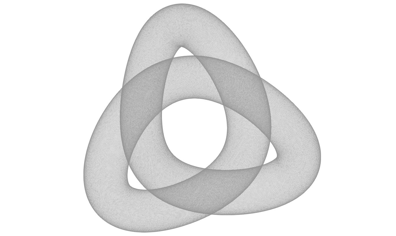
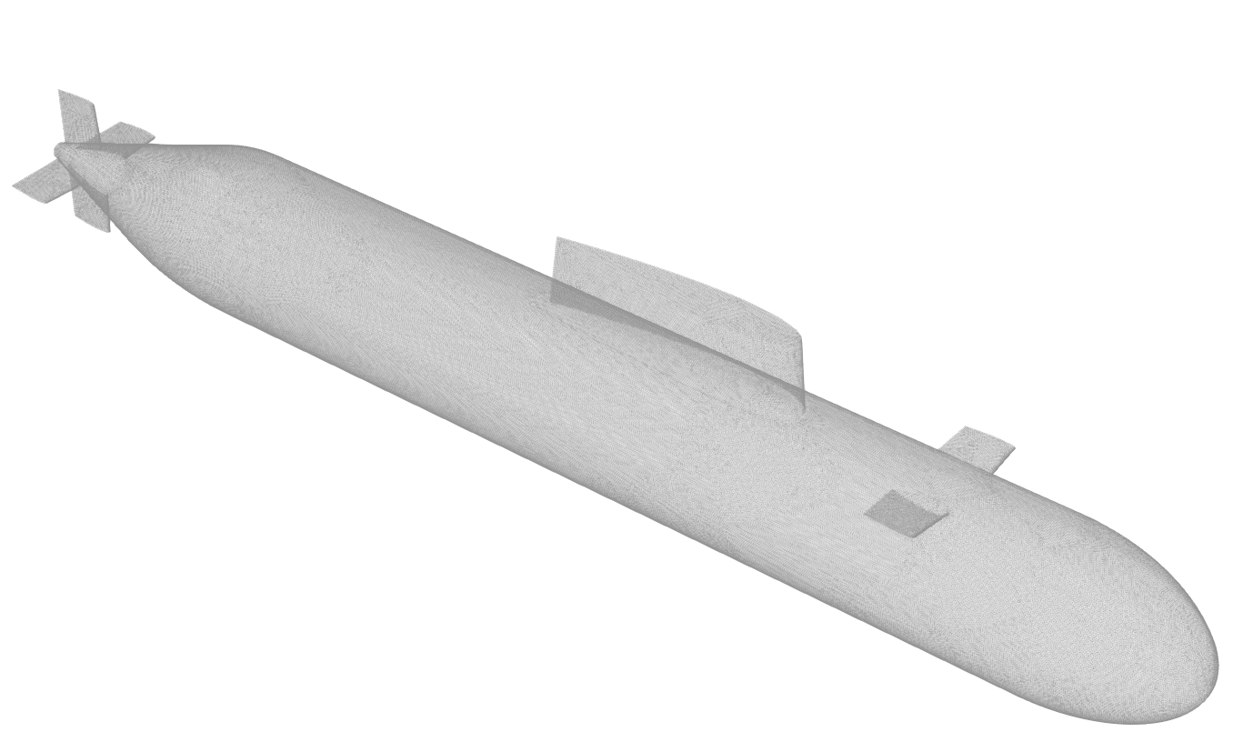
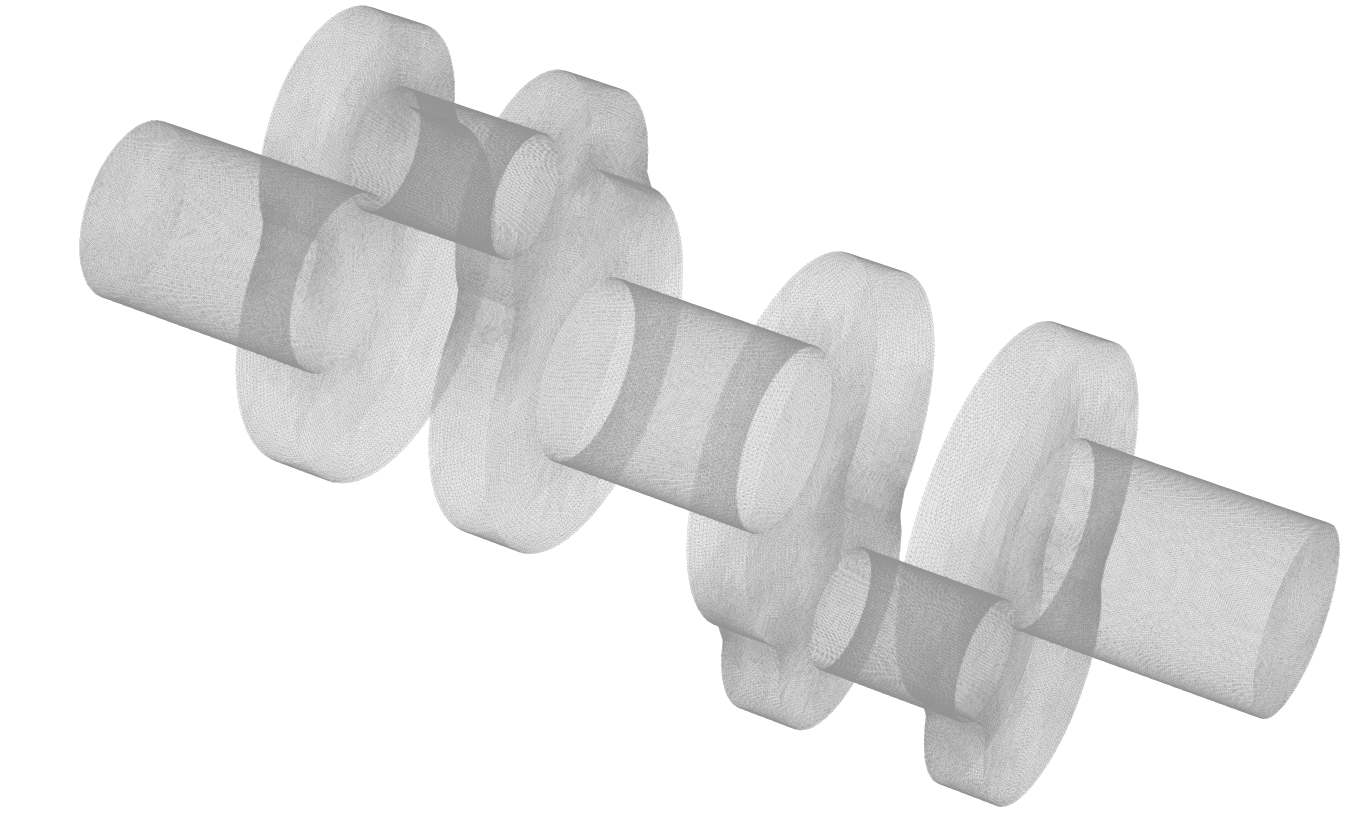
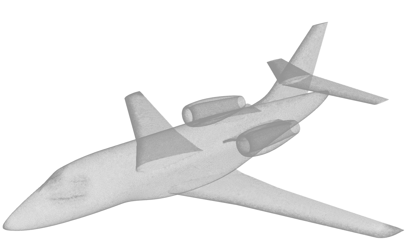
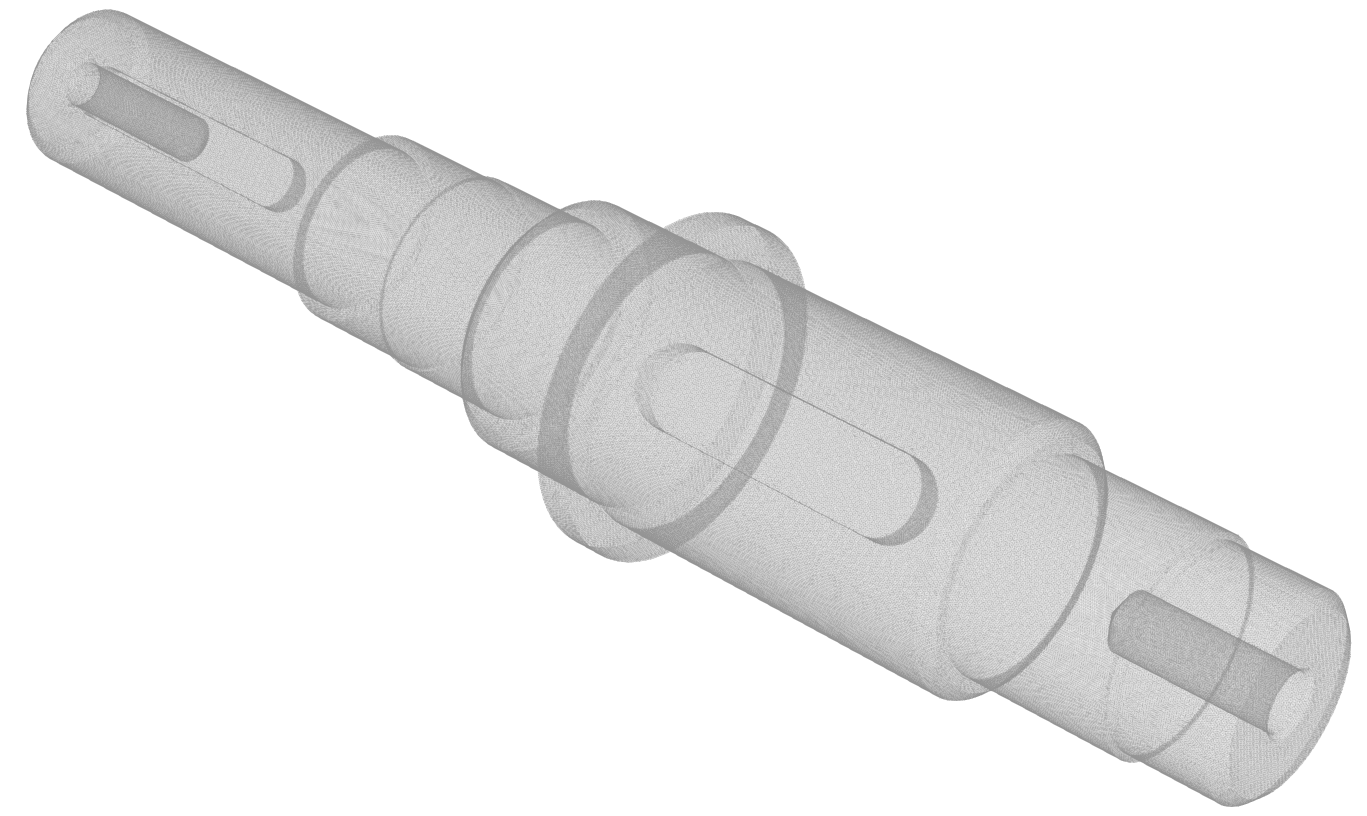
In the experiments, the single-layer boundary operator is considered on the sphere and on six additional shapes which we refer to as trefoil knot, submarine, crankshaft, frame, falcon and lathe part (see Figure 1). The sphere, trefoil knot and submarine are used at different levels of refinement.

Figure 1: Shapes used in the numerical experiments. From left to right and from top to bottom: trefoil knot ($548\,870\text{\,}\mathrm{t}\mathrm{r}\mathrm{i}\mathrm{a}\mathrm{n}\mathrm{g}\mathrm{l}\mathrm{e}\mathrm{s}$), submarine ($400\,886\text{\,}\mathrm{t}\mathrm{r}\mathrm{i}\mathrm{a}\mathrm{n}\mathrm{g}\mathrm{l}\mathrm{e}\mathrm{s}$), crankshaft ($672\,128\text{\,}\mathrm{t}\mathrm{r}\mathrm{i}\mathrm{a}\mathrm{n}\mathrm{g}\mathrm{l}\mathrm{e}\mathrm{s}$), frame ($451\,664\text{\,}\mathrm{t}\mathrm{r}\mathrm{i}\mathrm{a}\mathrm{n}\mathrm{g}\mathrm{l}\mathrm{e}\mathrm{s}$), falcon ($609\,104\text{\,}\mathrm{t}\mathrm{r}\mathrm{i}\mathrm{a}\mathrm{n}\mathrm{g}\mathrm{l}\mathrm{e}\mathrm{s}$) and lathe part ($535\,054\text{\,}\mathrm{t}\mathrm{r}\mathrm{i}\mathrm{a}\mathrm{n}\mathrm{g}\mathrm{l}\mathrm{e}\mathrm{s}$).

The Galerkin discretization requires a four-dimensional integral over a pair of mesh triangles for each element of the matrix. If these triangles touch or overlap, the integrals become (weakly) singular. Hence, Tensor-Gauss quadrature is employed where appropriate transformations from [40] map the quadrature nodes to the required domain of integration and remove the singularity in the singular cases. Unless specified otherwise, the chosen quadrature orders are $3$, $4$, $4$ and $5$ for separated, vertex-sharing, edge-sharing and identical triangles respectively.

For the cluster tree $\mathcal{T}_{I}=\mathcal{T}_{J}$, PCA is employed where clusters are split according to cardinality. A minimal leaf size of $30$ is chosen. Block cluster tree $\mathcal{T}_{{I\times I}}$ is built with subdivision strategy $s({\tau\times\sigma}):=s(\tau)\times s(\sigma)$. Admissibility is based on the weak admissibility criterion (7) using approximate diameters and distances based on axis-aligned bounding boxes. As $g$ is symmetric, so is the matrix after discretization; thus only admissible blocks below the diagonal are considered and each $\tau\in\mathcal{T}_{I}$ serves both as row and column cluster in accordance with Remark 4.

For construction, block-wise approximation is achieved using ACA with rook pivoting (ACA, see [20, §3.2] for more details). Relative tolerances are used for both ACA and the uniform compression. Given a specified tolerance $\epsilon$, the $\mathcal{H}$-matrix is constructed using $\epsilon$ as relative tolerance in ACA. To obtain (at least) similar accuracy, the $\mathcal{UH}$-matrix uses a tolerance of $\epsilon/3$ for ACA and uniform compression. Algebraic recompression of the blocks is performed with $\epsilon/10$ in both cases. Unless specified otherwise, $\epsilon$ is set to $10^{-4}$ in the experiments.

Remark 6 (Relative global error).

If one expects matrix $A$ to be “norm-balanced” in the sense that any submatrix ${A}_{|{\tau\times\sigma}}$ has spectral norm ${\|{A}_{|{\tau\times\sigma}}\|}_{2}\sim{\|A\|}_{2}\sqrt{{|\tau|\cdot|\sigma|}/{|I|\cdot|J|}}$, then Theorem 1 and the result in [29, Lemma 6.26] show that using a relative local tolerance $\epsilon$ results in a relative global error ${\|A-A^{\mathcal{UH}}\|}_{2}\lesssim{\|A\|}_{2}\epsilon$.

All experiments are performed on a compute node consisting of 2 Intel Xeon Platinum 8360Y (Ice Lake, 2.4 GHz) CPUs with 36 cores each, one L3 cache per CPU and 256 GiB total RAM. Parallel construction and matrix-vector multiplication using all 72 cores is achieved according to Subsection 4.4. Construction timings are performed 15 times while timing of the matrix-vector multiplication is run 500 times using three instances of the $\mathcal{H}$/$\mathcal{UH}$-matrix, for a total of 1500 runs. If not specified, the mean time over all runs is reported.

6.2 Sharpness of the admissibility criterion

The sparsity constant $c_{\mathrm{sp}}$ can have a significant impact on the attainable gains in compressing an $\mathcal{H}$-matrix to the $\mathcal{UH}$-matrix format. While $c_{\mathrm{sp}}$ is bounded independently of the matrix size, this bound is affected by several parameters. The bound based on geometrical observations in [1] depends on the geometry of the boundary and the local basis functions defined over it as well as on $\eta$ from the admissibility criterion (6) or (7). Intuitively, a larger value of $\eta$ will result in larger but fewer blocks being identified as admissible, thus decreasing $c_{\mathrm{sp}}$.

Figure 2 shows the memory usage of both the $\mathcal{H}$-matrix and $\mathcal{UH}$-matrix as a function of $\eta$ for the trefoil knot and the crankshaft at wavenumbers defined relative to the largest triangle side-length $h$ in each shape.

Figure 2: Memory usage as a function of $\eta$ for the trefoil knot ($\kappa h=0.1$, left) and crankshaft ($\kappa h=0.4$, right) in regular and uniform $\mathcal{H}$-matrix format.

In both cases, the total memory usage decreases to an asymptote with increasing $\eta$. The case $\eta\to\infty$ could be understood as considering a block admissible if its clusters’ bounding boxes do not overlap. In the case of the $\mathcal{H}$-matrix, both the admissible and dense storage contributions benefit from relaxing the admissibility criterion. The dense storage reduces as blocks turn admissible while the admissible storage reduces as children blocks are aggregated into a parent block with less memory usage. The aggregation directly results in a lower sparsity constant. The $\mathcal{UH}$-matrix format is affected by this to the point where increase of $\eta$ leads to increase of the admissible block storage. We observe that the $\mathcal{UH}$-matrix is less affected by a poor choice of $\eta$, which can be seen as a qualitative advantage as it becomes easier to choose a ‘good’ value of $\eta$.

Based on Figure 2, $\eta=10$ is chosen for the remainder of the experiments.

6.3 Asymptotics in the problem size

To verify the log-linear complexity of the compression scheme, it is applied to three sets of iteratively refined meshes. Figure 3 shows the memory usage and construction time for the trefoil knot over a range of refinements. This is done for the Laplace kernel, obtained by setting $\kappa=0$, as well as for the Helmholtz kernel with $\kappa h=0.3$. Both the sequential and parallel construction times are reported, except for the largest meshes.

Figure 3: Memory usage and construction time as a function of $N$ for the trefoil knot in regular and uniform $\mathcal{H}$-matrix format at $\kappa h=0$ (blue) and $\kappa h=0.3$ (orange).

Considering the memory usage of both the $\mathcal{H}$-matrix and $\mathcal{UH}$-matrix, the complexity is clearly $\mathcal{O}(N\log N)$ in the case of the Laplace kernel. Given that $\kappa$ increases with $N$ if $\kappa h\sim 1$, it is not expected that the Helmholtz kernel scales as $\mathcal{O}(N\log N)$; however it remains close here. The construction time scales similarly except for the parallel construction at the largest $N$, where additional memory-architecture effects play a role. Noteworthy is the observation that the $\mathcal{UH}$-matrix construction not only scales with $\mathcal{O}(N\log N)$ as expected but also parallelizes equally well as the $\mathcal{H}$-matrix construction.

Table 6.3 compiles the results of the sphere and the submarine for $\kappa=0$. Similar observations can be made w.r.t. the complexity as in Figure 3. The $\mathcal{UH}$-matrix is able to attain compression factors close to 2 while the construction time is comparable. Table 6.3 can be compared to [10, Table 4.2] where $\mathcal{H}$-matrices are compressed to the $\mathcal{H}^{2}$-matrix format. For larger $N$, the linear storage complexity of $\mathcal{H}^{2}$-matrices results in larger compression ratios than reported here. However, the total construction time still scales log-linearly. Due to the recursive $\mathcal{H}^{2}$-matrix structure, the compression scheme is also much more involved and requires more implementation effort.

[ head to column names, tabular = ccccccc, table head = $\mathcal{H}$-matrix $\mathcal{UH}$-matrix
$N$ $\mathrm{Mem}/N$ Build(1) Build(72) $\mathrm{Mem}/N$ Build(1) Build(72)
, table foot = , ]data/discretization/sphere-laplace-seq/merged-table.csv $\fpeval{3*\NtP}$ $\fpeval{\memperdofHP/1e3}$ $\minBuildHS$ $\minBuildHP$ $\fpeval{\memperdofUP/1e3}$ $\minBuildUS$ $\minBuildUP$ [ head to column names, tabular = ccccccc, table head = $N$ $\mathrm{Mem}/N$ Build Build $\mathrm{Mem}/N$ Build Build
, table foot = , ]data/discretization/beTSSi-laplace-seq/merged-table.csv $\fpeval{3*\NtP}$ $\fpeval{\memperdofHP/1e3}$ $\minBuildHS$ $\minBuildHP$ $\fpeval{\memperdofUP/1e3}$ $\meanBuildUS$ $\meanBuildUP$

Table 1: Memory usage per degree of freedom in KB and construction time (sequential and parallel) in seconds for the increasingly refined sphere (top) and submarine (bottom) at $\kappa=0$.

6.4 Behavior with respect to tolerance

The storage cost and construction time of $\mathcal{H}$- and $\mathcal{UH}$-matrices implicitly depend on the tolerance through the block ranks $(k_{b})_{b}$ and cluster ranks $(\ell_{\tau})_{\tau}$ and $(\ell_{\sigma})_{\sigma}$. Figure 4 shows the memory usage and construction time as a function of the relative tolerance $\epsilon$ for the crankshaft and submarine. Default quadrature orders of $(3,4,4,5)$ were used at precisions $10^{-3}$ and $10^{-4}$ while they were increased to $(4,5,5,6)$ for $\epsilon=10^{-5}$ and decreased to $(2,3,3,4)$ for $\epsilon=10^{-2}$.

Figure 4: Memory usage and parallel construction time as a function of the tolerance $\epsilon$ for the crankshaft and submarine at $\kappa h=0.1$ in regular and uniform $\mathcal{H}$-matrix format. Left: Absolute values for the crankshaft. Middle: Absolute values for the submarine. Right: Relative values $\mathcal{H}/\mathcal{UH}$.

The memory usage of both the $\mathcal{H}$-matrix and $\mathcal{UH}$-matrix behave as $\mathcal{O}(\log(1/\epsilon))$. This is expected as the asymptotic smoothness of the kernel results in exponentially decaying singular values of the admissible blocks. The compression factors are stable throughout the $\epsilon$-range.

The expected behavior of the construcion time w.r.t. the tolerance is more complicated as different parts of the construction have rank dependencies of $k$, $k^{2}$ and $k^{3}$. Additionally, as the sampling of the matrix elements has a $\mathcal{O}(q^{4})$ dependence on the quadrature order $q$, this affects the construction time as well, which is very pronounced at $\epsilon=10^{-5}$. For both shapes, the $\mathcal{UH}$-matrix construction is generally faster as the reduction in memory overhead outweighs the computational cost of the compression.

6.5 Memory reduction in the $\mathcal{UH}$-matrix format

As a final experiment, the robustness of the uniform compression is tested by applying it to a total of six shapes with varying values for $\kappa h$. The results are put together in Table 6.5. The $\mathcal{H}$-matrix results are given in absolute values while the $\mathcal{UH}$-matrix results are given in relative terms.

[ head to column names, tabular = ¿lccccccccc, table head = $\mathcal{H}$-matrix Improvement factor $\mathcal{H}/\mathcal{UH}$
Shape $N$ $\kappa h$ $\mathrm{Mem_{tot}}$ Build MV $\mathrm{Mem_{tot}}$ $\mathrm{Mem_{adm}}$ Build MV
, table foot = , ]data/meshStats/paper-v1/compression_table-reordered.csv $\fpeval{3*\NtH}$ $\khH$ $\fpeval{\memtotH/1e9}$ $\meanBuildH$ $\meanMatvecH$ $\fpeval{\memtotH/\memtotU}$ $\fpeval{\memadmH/\memadmU}$ $\fpeval{\meanBuildH/\meanBuildU}$ $\fpeval{\meanMatvecH/\meanMatvecU}$ Throughout the shapes, the $\mathcal{UH}$-matrix format is able to compress the admissible memory with a factor between $2$ and $3$. As a result, the total memory usage sees a reduction around $1.9$. This is similar to the factors that can be inferred from the previous experiments.

Table 2: Memory usage in GB, and parallel construction time and matrix-vector product timings (MV) in seconds for the $\mathcal{H}$- and $\mathcal{UH}$-matrix of six different shapes.

The additional construction cost is manageable. In the worst case, i.e. the falcon, the uniform compression only increases the total construction time by 25%. In some cases, here for the crankshaft but also seen in e.g. Figure 4, the construction time is improved, which may be attributed to the lower memory usage throughout the construction.

The memory reduction positively influences the performance of the matrix-vector products. For both formats, these are done in parallel (see Algorithm 5 and 6). While these factors are lower than the actual compression, they still indicate that the parallelizability of the $\mathcal{UH}$-matrix-vector product is comparable – at least in a simple parallel implementation – to that of the regular $\mathcal{H}$-matrix.

7 Conclusion and future work

We have shown that $\mathcal{H}$-matrices can be cheaply compressed to the uniform $\mathcal{H}$-matrix format in an algebraic manner. This approximately halves the total memory usage in the process. By incorporating the initial $\mathcal{H}$-matrix construction into the compression, a $\mathcal{UH}$-matrix can be constructed directly without the need to store the intermediate $\mathcal{H}$-matrix. Using this approach, the construction time of the $\mathcal{UH}$-matrix is comparable to that of the $\mathcal{H}$-matrix. The more compact $\mathcal{UH}$-matrix also results in a faster matrix-vector product.

Future work include experiments on a wider variety of matrices, among which different BEM matrices and a direct comparison with the $\mathcal{H}^{2}$-matrix compression. Additionally, we plan to apply the ideas of the uniform compression to the compact representation for wavenumber-dependent BEM matrices in [21].

References

- [1] Bebendorf, M. Hierarchical matrices: a means to efficiently solve elliptic boundary value problems, 1st ed., vol. 63 of Lecture Notes in Computational Science and Engineering. Springer, Berlin, Heidelberg, 2008.
- [2] Bebendorf, M., and Hackbusch, W. Existence of -matrix approximants to the inverse FE-matrix of elliptic operators with -coefficients. Numer. Math. 95, 1 (2003), 1–28.
- [3] Bebendorf, M., and Kriemann, R. Fast parallel solution of boundary integral equations and related problems. Comput. Vis. Sci. 8, 3-4 (2005), 121–135.
- [4] Bebendorf, M., and Kunis, S. Recompression techniques for adaptive cross approximation. J. Integral Equ. Appl. 21, 3 (2009), 331–357.
- [5] Bebendorf, M., and Rjasanow, S. Adaptive low-rank approximation of collocation matrices. Computing 70, 1 (2003), 1–24.
- [6] Bruyninckx, K., Dirckx, S., Huybrechs, D., and Meerbergen, K. A wavenumber-dependent representation and frequency sweeping method for the 3D Helmholtz equation using discontinuous Galerkin BEM. in preparation.
- [7] Börm, S. Approximation of integral operators by -matrices with adaptive bases. Computing 74, 3 (2005), 249–271.
- [8] Börm, S. Adaptive variable-rank approximation of general dense matrices. SIAM J. Sci. Comput. 30, 1 (2007), 148–168.
- [9] Börm, S. Data-sparse approximation of non-local operators by -matrices. Linear Algebra Appl. 422, 2 (2007), 380–403.
- [10] Börm, S. Construction of data-sparse -matrices by hierarchical compression. SIAM J. Sci. Comput. 31, 3 (2009), 1820–1839.
- [11] Börm, S. Approximation of solution operators of elliptic partial differential equations by - and -matrices. Numer. Math. 115, 2 (2010), 165–193.
- [12] Börm, S. Directional ‐matrix compression for high‐frequency problems. Numer. Linear Algebra Appl. 24, 6 (2017).
- [13] Börm, S., and Borst, C. Hybrid matrix compression for high-frequency problems. SIAM J. Matrix Anal. Appl. 41, 4 (2020), 1704–1725.
- [14] Börm, S., and Christophersen, S. Approximation of integral operators by Green quadrature and nested cross approximation. Numer. Math. 133, 3 (2016), 409–442.
- [15] Börm, S., and Grasedyck, L. Low-rank approximation of integral operators by interpolation. Computing 72, 3-4 (2004), 325–332.
- [16] Börm, S., and Grasedyck, L. Hybrid cross approximation of integral operators. Numer. Math. 101, 2 (2005), 221–249.
- [17] Börm, S., and Hackbusch, W. Approximation of boundary element operators by adaptive -matrices. Found. Comput. Math. 312 (2004), 58–75.
- [18] Börm, S., and Henningsen, J. Memory-efficient compression of -matrices for high-frequency problems, 2023. arXiv:2310.00111. Retrieved from https://arxiv.org/abs/2310.00111.
- [19] Börm, S., Lohndorf, M., and Melenk, J. M. Approximation of integral operators by variable-order interpolation. Numer. Math. 99, 4 (2005), 605–643.
- [20] Dirckx, S. Efficient Representations of Wavenumber Dependent BEM Matrices: Construction and Analysis for the 3D Scalar Helmholtz Equation. PhD thesis, Leuven, Belgium, 2024.
- [21] Dirckx, S., Huybrechs, D., and Meerbergen, K. Frequency extraction for BEM matrices arising from the 3D scalar Helmholtz equation. SIAM J. Sci. Comput. 44, 5 (2022), B1282–B1311.
- [22] Fong, W., and Darve, E. The black-box fast multipole method. J Comput Phys 228, 23 (2009), 8712–8725.
- [23] Golub, G. H., and van Loan, C. F. Matrix Computations, 4th ed. JHU Press, Philadelphia, PA, 2013.
- [24] Grasedyck, L. Adaptive recompression of -matrices for BEM. Computing 74, 3 (2005), 205–223.
- [25] Grasedyck, L., and Hackbusch, W. Construction and arithmetics of -matrices. Computing 70, 4 (2003), 295–334.
- [26] Greengard, L. The rapid evaluation of potential fields in particle systems. PhD thesis, New Haven, CT, USA, 1987. AAI 8727216.
- [27] Greengard, L., and Rokhlin, V. A fast algorithm for particle simulations. J. Comput. Phys. 73, 2 (1987), 325–348.
- [28] Hackbusch, W. A sparse matrix arithmetic based on -matrices. part I: Introduction to -matrices. Computing 62, 2 (1999), 89–108.
- [29] Hackbusch, W. Hierarchical matrices: algorithms and analysis, 1st ed., vol. 49 of Springer Series in Computational Mathematics. Springer, Berlin, Heidelberg, 2015.
- [30] Hackbusch, W., and Börm, S. Data-sparse approximation by adaptive -matrices. Computing 69, 1 (2002), 1–35.
- [31] Hackbusch, W., and Nowak, Z. On the fast multiplication in the boundary element method by panel clustering. Numer. Math. 54 (07 1989), 463–491.
- [32] Hoshino, T., Ida, A., and Hanawa, T. Optimizations of H-matrix-vector multiplication for modern multi-core processors. In IEEE International Conference on Cluster Computing (Piscataway, 2022), IEEE, pp. 462–472.
- [33] Kriemann, R. Hierarchical lowrank arithmetic with binary compression, 2023. arXiv:2308.10960v1. Retrieved from https://arxiv.org/abs/2308.10960v1.
- [34] Letourneau, P.-D., Cecka, C., and Darve, E. Cauchy fast multipole method for general analytic kernels. SIAM J. Sci. Comput. 36, 2 (2014), A396–A426.
- [35] Mclean, W. Strongly elliptic systems and boundary integral equations. Cambridge University Press, Cambridge, 2000.
- [36] Murray, R., Demmel, J., Mahoney, M. W., Erichson, N. B., Melnichenko, M., Malik, O. A., Grigori, L., Luszczek, P., Dereziński, M., Lopes, M. E., Liang, T., Luo, H., and Dongarra, J. Randomized numerical linear algebra : A perspective on the field with an eye to software. arXiv:2302.11474v2. Retrieved from https://arxiv.org/abs/2302.11474v2.
- [37] Pearson, K. On lines and planes of closest fit to systems of points in space. Philos. Mag. 2, 11 (1901), 559–572.
- [38] Rokhlin, V. Rapid solution of integral equations of classical potential theory. J. Comput. Phys. 60, 2 (1985), 187–207.
- [39] Sauter, S. Variable order panel clustering. Computing 64, 3 (2000), 223–261.
- [40] Sauter, S. A., and Schwab, C. Boundary Element Methods, 1st ed., vol. 39 of Springer Series in Computational Mathematics. Springer, Berlin, Heidelberg, 2011.
- [41] Ying, L., Biros, G., and Zorin, D. A kernel-independent adaptive fast multipole algorithm in two and three dimensions. J. Comput. Phys. 196, 2 (2004), 591–626.