Error Crafting in Probabilistic Quantum Gate Synthesis

Nobuyuki Yoshioka nyoshioka@ap.t.u-tokyo.ac.jp Department of Applied Physics, University of Tokyo, 7-3-1 Hongo, Bunkyo-ku, Tokyo 113-8656, Japan Theoretical Quantum Physics Laboratory, RIKEN Cluster for Pioneering Research (CPR), Wako-shi, Saitama 351-0198, Japan JST, PRESTO, 4-1-8 Honcho, Kawaguchi, Saitama, 332-0012, Japan    Seiseki Akibue NTT Communication Science Laboratories, NTT Corporation, Atsugi 243-0198, Japan    Hayata Morisaki Graduate School of Engineering Science, Osaka University 1-3 Machikaneyama, Toyonaka, Osaka 560-8531, Japan    Kento Tsubouchi Department of Applied Physics, University of Tokyo, 7-3-1 Hongo, Bunkyo-ku, Tokyo 113-8656, Japan    Yasunari Suzuki NTT Computer and Data Science Laboratories, NTT Corporation, Musashino 180-8585, Japan
Abstract

At the early stage of fault-tolerant quantum computing, it is envisioned that the gate synthesis of a general unitary gate into universal gate sets yields error whose magnitude is comparable with the noise inherent in the gates themselves. While it is known that the use of probabilistic synthesis already suppresses such coherent errors quadratically, there is no clear understanding on its remnant error, which hinders us from designing a holistic error countermeasure that is effectively combined with error suppression and mitigation. In this work, we propose that, by exploiting the fact that synthesis error can be characterized completely and efficiently, we can craft the remnant error of probabilistic synthesis such that the error profile satisfies desirable properties. We prove for the case of single-qubit unitary synthesis that, there is a guaranteed way to perform probabilistic synthesis such that we can craft the remnant error to be described by Pauli and depolarizing errors, while the conventional twirling cannot be applied in principle. Furthermore, we show a numerical evidence for the synthesis of Pauli rotations based on Clifford+T formalism that, we can craft the remnant error so that it can be eliminated up to cubic order by combining logical measurement and feedback operations. As a result, Pauli rotation gates can be implemented with T counts of $\log_{2}(1/\varepsilon)$ on average up to accuracy of $\varepsilon=10^{-9}$, which can be applied to early fault-tolerant quantum computation beyond classical tractability. Our work opens a novel avenue in quantum circuit design and architecture that orchestrates error countermeasures.

Introduction

It is widely accepted that quantum computers with error correction [1, 2] can be potentially useful in various tasks such as factoring [3], quantum many-body simulation [4], quantum chemistry [5], and machine learning [6]. With the tremendous advancements in the quantum technology, the earliest experimental demonstrations of quantum error correction are realized with various codes  [7, 8, 9, 10, 11, 12, 13, 14, 15]. While such a progress towards fault-tolerant quantum computing (FTQC) is promising, quantum computers in the coming generation, the early fault-tolerant quantum computers, would still be subject to noise at the logical level, and hence the error countermeasures developed for noisy intermediate-scale quantum (NISQ) devices, in particular the quantum error mitigation (QEM) techniques [16, 17, 18, 19, 20, 21, 22, 23], will remain essential to exemplify practical quantum advantage [24, 25, 26, 27, 28, 29, 30]. Meanwhile, there is a stark difference between (early) FTQC and NISQ regimes that is characterized by the Eastin-Knill theorem [31]; the universal gate set is discrete. This indicates that the gate synthesis yields coherent error whose effect is comparable to incoherent errors triggered by noise in the hardware.

In contrast to incoherent errors which inevitably necessitate entropy reduction via measurement and feedback [32, 33, 34, 35], there is no corresponding fundamental limitation for coherent errors. In fact, several previous works have found that algorithmic errors can be dealt more efficiently than naive expectation [36, 37, 38, 39, 40, 41]. It was pointed out by Refs. [36, 37] that, when one have access to a Pauli rotation exposed to over and under rotations, we can simply take probabilistic mixture of two to achieve quadratic suppression of the error. Such findings have invoked the proposal of a probabilistic gate synthesis algorithm that approximately halves the consumption of magic gates under single-qubit unitary synthesis [39, 41]. It must be noted that, these existing works merely focus on the accuracy of the probabilistic synthesis, while one must take care of the compatibility between other error countermeasures to further suppress the errors. This is prominent when one desires to perform an unbiased computation via the QEM, which requires a deep knowledge of the error channel. To our knowledge, however, there is no firm understanding on the remnant error channel nor attempt to control the profile of them.

In this work, we make a first step to fill this gap by introducing a notion of error crafting, i.e., perform the probabilistic synthesis that results in a remnant error channel with a desired property, for single-qubit unitaries synthesized under the framework of Clifford+T formalism. We rigorously prove that one can design the synthesis protocol to assure the remnant error to be constrained to Pauli error, which is crucial to perform efficient error mitigation techniques [16, 17, 25]. We further provide a numerical evidence that, in the case of Pauli rotation gates, one can reliably manipulate the remnant error to be biased. This allows us to perform error detection at the logical level which achieves quadratically small sampling overhead compared to the existing lower bound of sample complexity that does not rely on mid-circuit measurement. We furthermore extend our framework to perform error crafting using CPTP channels obtained from error correction at logical layer, and show that the remnant error can be suppressed up to cubic order. As a result, we can implement Pauli rotation gates of accuracy $\varepsilon$ with T count of $\log_{2}(1/\varepsilon)$ up to $\varepsilon=10^{-9}$, which is expected to be sufficient for various medium-scale FTQC beyond state-of-the-art classical computation [27, 28, 26, 30].

We remark that the operation of twirling shares the spirit of transforming a noise channel into another channel with better-known property via randomized gate compilation. However, there are two severe limitations in twirling: first, it agnostically smears out the characteristics of the channel, and second, it cannot be applied to noise maps following non-Clifford operations in general. This is in sharp contrast to our work, since our objective is to fully utilize the information on the error profile of general unitary synthesis that can be characterized completely and efficiently via classical computation.

Unitary, probabilistic, and error-crafted synthesis

We aim to implement a target single-qubit unitary $\hat{U}$ with its channel representation given by $\hat{\mathcal{U}}$. We hereafter distinguish the unitaries before and after synthesis by the presence and absence of a hat. Due to the celebrated Eastin-Knill’s theorem [31], there is no fault-tolerant implementation of continuous gate sets, and therefore we cannot exactly implement the target in general. We alternatively aim to approximate $\hat{U}$ by decomposing it to a sequence of implementable operations. Such a task is called gate synthesis.

One of the most common approaches for gate synthesis is the unitary synthesis, namely to decompose the target unitary into sequence of implementable unitary gate sets. For instance, unitary synthesis into the Clifford+T gate set is known to be possible with classical computation time of $O({\rm polylog}(1/\epsilon))$ for arbitrary single-qubit Pauli rotation assuming a factoring oracle [42] and $O({\rm poly}(1/\epsilon))$ for a general SU(2) gate [43, 44]. Another measure for the efficiency of synthesis is the number of T gates, or the T count, since T gates require cumbersome procedures such as magic state distillation and gate teleportation. In this regard, the existing methods saturates the information-theoretic lower bound regarding the T count of $3\log_{2}(1/\epsilon)$ except for rare exceptions that require $4\log_{2}(1/\epsilon)$ [45, 42, 43, 44].

We may also consider probabilistic synthesis, which takes probabilistic mixture of several different outputs from the unitary synthesis algorithm. Concretely, we generate a set of slightly shifted unitaries $\{U_{j}\}$ which are $\epsilon$-close approximations of the target unitary $\hat{U}$ in terms of diamond distance as $d_{\diamond}(\hat{\mathcal{U}},\mathcal{U}_{j})\leq\epsilon$ (see Supplementary Note S1 for the definition of diamond distance). It is known that the probabilistic synthesis allows quadratic suppression of the error, when we appropriately generate a set of synthesized unitaries $\{\mathcal{U}_{j}\}$ and choose the probability distribution over them:

Lemma 1.

(informal [41]) Let $\hat{\mathcal{U}}$ be a target unitary channel with $\{\mathcal{U}_{j}\}$ constituting its $\epsilon$-net in terms of the diamond distance. Then, one can find the optimal probabilistic compilation $\{p_{j}\}$ such that the diamond distance is bounded as

$\displaystyle d_{\diamond}\bigg{(}\hat{\mathcal{U}},\sum_{j}p_{j}\mathcal{U}_{j}\bigg{)}\leq\epsilon^{2},$ (1)

by solving the following minimization problem via semi-definite programming:

$\displaystyle p=\underset{p}{\operatorname{argmin}}~{}d_{\diamond}\bigg{(}\hat{\mathcal{U}},\sum_{j}p_{j}\mathcal{U}_{j}\bigg{)}.$ (2)

As an extension of existing synthesis techniques, here we propose error-crafted synthesis, or error crafting. In short, this can be understood as constraining the remnant error of the synthesis, depending on the subsequent error countermeasure (such as QEM or error detection) one wish to perform. We formally define the remnant error channel as

$\displaystyle\mathcal{E}_{\rm rem}(\cdot)=\left(\sum_{j}p_{j}\Lambda_{j}\right)\circ\hat{\mathcal{U}}^{-1}(\cdot)=\sum_{ab}\chi_{ab}P_{a}\cdot P_{b},$ (3)

where $P_{a}\in\{{\rm I},{\rm X},{\rm Y},{\rm Z}\}$ and $\{\chi_{ab}\}$ gives the chi representation of the remnant error. We also allow the implementable channel to be non-unitary CPTP map as $\{\Lambda_{j}\},$ which we find to be useful when we incorporate measurement and feedback as discussed later. The aim of the crafted synthesis is to control $\{\chi_{ab}\}$ by optimizing the probability distribution $\{p_{j}\}$ for appropriately generated $\{\Lambda_{j}\}$.

Let us remark that we require the synthesis protocol to be distinct from the QEM stage, in a sense that we do not allow synthesis to increase the sampling overhead, the multiplication factor in the number of circuit execution. Also, we require that the gate complexity is nearly homogeneous even if we include feedback operations, in order to prevent a situation where parallel application of multiple synthesized channels is stalled due to a fallback scheme [46, 39].

Refer to caption
Figure 1: Numerical analysis on error-crafted synthesis for the Pauli constraint. (a) Diamond distance $d_{\diamond}(\hat{\mathcal{U}},\mathcal{U}_{\rm synth})$ between the target single-qubit Haar random unitary $\hat{\mathcal{U}}$ and the synthesized channel $\mathcal{U}_{\rm synth}\coloneqq\sum_{j}p_{j}\mathcal{U}_{j}$. The black real line indicates the results from unitary synthesis by the Ross-Selinger algorithm, while the filled dots are results from probabilistic synthesis with shift factors of $c=2,3,5,7.$ When we increase the number of synthesized unitaries by a factor of $R=3$ for $c=7$, shown by unfilled triangles, the remnant synthesis error is suppressed below the bound in Eq. (5) and approaches the value of $\epsilon^{2}$, which matches the upper bound for the non-constrained case as in Eq. (1). The plots are averaged over 200 trials. (b) Surface plot of failure rate $p_{\rm fail}$ of probabilistic synthesis under the Pauli constraint, averaged over 200 trials for $\epsilon=10^{-4}.$ Scaling with $c$ and $R$ are shown in (c), (d), where the number of data is 10000 and 2000, respectively.

Crafting remnant error to be Pauli channel

While the quadratic suppression (1) by probabilistic synthesis is already beneficial for practical quantum computing, the performance of many error counteracting protocol can be enhanced when we craft the remnant error $\mathcal{E}_{\rm rem}$. For instance, let us consider the probabilistic error cancellation (PEC), which is one of the most well-known error mitigation techniques that estimates expectation values of physical observables by quasiprobabilistic implementation of error channel inversion [16, 47]. One can show that it suffices to take Clifford operations and Pauli initialization to constitute a universal set to invert arbitrary single-qubit error channels [18, 48], while the implementation is significantly simplified when $\mathcal{E}_{\rm rem}$ is a Pauli channel. This is because the PEC can be performed merely via updates on Pauli frames, which is purely done by classical processing of stabilizer measurements [25]. As another example, when we consider the rescaling technique under white-noise approximation [49, 50], which is a provably cost-optimal way of error mitigation, we can drastically improve the accuracy of the approximation when the errors are free from coherent components (see Supplementary Note S5 for details).

In this regard, we make a further step and ask the following question: can we guarantee both quadratic error suppression and success of crafting the remnant error to be Pauli channel? This is equivalent to solving the following optimization problem:

$\displaystyle{\rm minimize}~{}d_{\diamond}\left(\hat{\mathcal{U}},\sum_{j}p_{j}\mathcal{U}_{j}\right)~{}{\rm s.t.}~{}\mathcal{E}_{\rm rem}(\cdot)=\sum_{a}\chi_{aa}P_{a}\cdot P_{a},$ (4)

where $\chi_{aa}\geq 0$ is required for all $a$. We emphasize that this cannot be achieved by naively applying twirling techniques, since randomization for coherent errors following non-Clifford unitary demands non-Clifford operations, which are not error-free in FTQC. Our strategy is to prepare shift unitaries $\{\mathcal{V}_{j}^{c\epsilon}\}_{j}$ that can be used to generate a set of $c\epsilon$-close unitaries such that the feasibility of the minimization problem (4) is assured even when unitary synthesis induces error of $\epsilon$. By explicitly constructing such a set of shift unitaries, we rigorously answer to the above-raised question as the following:

Theorem 1.

There exist shift factor $c$, a positive number $\epsilon_{0}$, and a set of shift unitaries $\{\mathcal{V}_{j}^{c\epsilon}\}_{j=1}^{7}$ such that, for any given single-qubit unitary $\hat{\mathcal{U}}$ and for any $\epsilon\in(0,\epsilon_{0}]$, if we synthesize the shifted target unitaries to obtain $\{\mathcal{U}_{j}\}=\{\mathcal{A}(\mathcal{V}_{j}^{c\epsilon}\circ\hat{\mathcal{U}})\}$ so that $d_{\diamond}(\mathcal{V}_{j}^{c\epsilon}\circ\hat{\mathcal{U}},\mathcal{U}_{j})\leq\epsilon$ is satisfied under the synthesis algorithm $\mathcal{A}$, then there exists probabilistic mixture of $\{\mathcal{U}_{j}\}$ that induces a Pauli channel as the effective synthesis error, with the accuracy being

$$(c-1)^{2}\epsilon^{2}\leq d_{\diamond}\bigg{(}\hat{\mathcal{U}},\sum_{j}p_{j}\mathcal{U}_{j}\bigg{)}\leq(c+1)^{2}\epsilon^{2}.$$ (5)

Remarkably, this theorem states that we can craft the error without assuming anything but the accuracy for the synthesis algorithm $\mathcal{A}$. It is also worth noting that the minimization problem (4) can be solved by the linear programming.

To prove Theorem 1, we explicitly construct the shift unitaries $\{\mathcal{V}_{j}^{c\epsilon}\}_{j}$, and show that the feasibility of the solution is robust even under additional synthesis error of $\epsilon.$ Once such a solution is assured, the upper bound of Eq. (5) follows directly from the formulation via the minimization over diamond distance and the fact that $\{\mathcal{U}_{j}\}_{j=1}^{7}$ is $(c+1)\epsilon$-close to $\hat{\mathcal{U}}$ with respect to the diamond distance. Also, the lower bound follows from the fact that the diamond distance between the compiled shifted unitaries $\{\mathcal{U}_{j}\}$ and the target unitary $\hat{\mathcal{U}}$ are at least $(c-1)\epsilon$. We guide readers to Supplementary Note S6 for details of the proof.

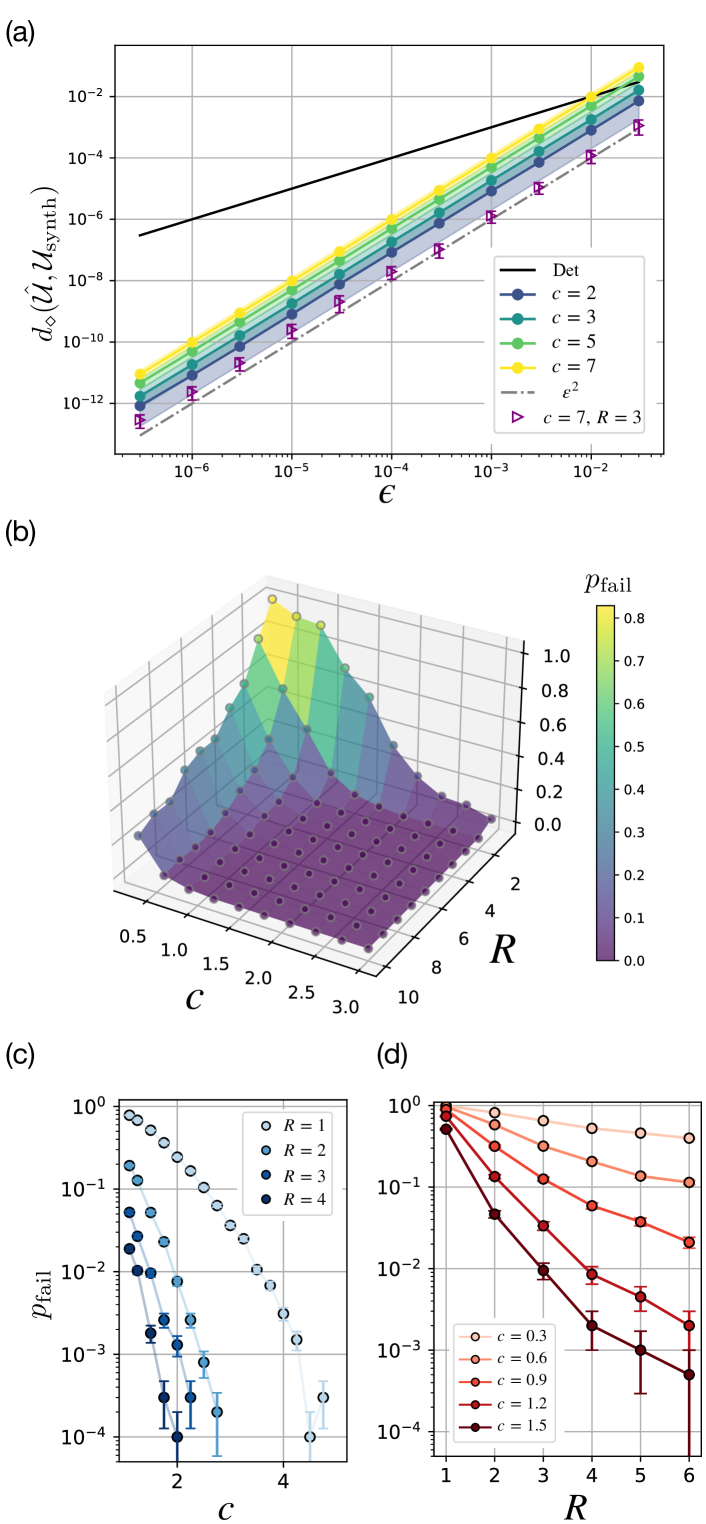
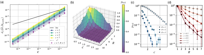
Since the theorem only states the existence of finite $c$, we rely on numerical simulation to assure the practical usage with finite $c$ values. For this purpose, we synthesize a single-qubit Haar random unitary gate by first performing the axial decomposition into three Pauli rotations, each of which passed to the synthesis algorithm proposed by Ross and Selinger [42]. As shown in Fig. 1(a), the probabilistic synthesis indeed yields error-bounded solutions that achieve quadratic suppression compared to the unitary synthesis. Meanwhile, we find that the Pauli constraint is violated when we take small shift factors $c$. This is not contradicting Theorem 1, since the theorem only states the existence of $c$ which always yield successful results. It must be noted that, as shown in Fig. 1(b) and (c), the occurrence of such a violation is suppressed exponentially by increasing the value of $c$. We observe that it suffices to take $c\sim 3.5,4.5$ to yield feasible solution with failure probability of $10^{-2},10^{-3}$, respectively, and naturally deduce that $c\sim 5.5,6.5$ is required to reach $10^{-4},10^{-5}.$ We remark that, while we have employed the axial decomposition of the SU(2) gates for the results shown here, we observe similar suppression when we utilize a direct synthesis algorithm [51].

Refer to caption
Figure 2: Numerical analysis on error crafting for remnant errors. Here we display the distribution of error rate ratio $(q_{x},q_{y},q_{z})=(p_{x}/p,p_{y}/p,p_{z}/p)$ with constraints on error profile. The unitary synthesis is done for $\epsilon=10^{-4}$ with shift factor $c=2.0,5.0$ for depolarizing and XY constraints, respectively.

Since increasing the shift factor $c$ increases the prefactor of the remnant error by $c^{2}$, we find it beneficial to introduce another practical strategy that enhances the feasibility of the solution. Here we provide a simple yet powerful technique; by generating the shift unitaries for $R$ different shift factors $c/R,2c/R,...,c$ and solving the problem with $R$-fold larger number of basis set, we can both suppress the failure of error-crafted synthesis (see Fig. 1(b) and (d)) and the remnant error. As shown in Fig. 1(a), when we take $c=7$ and $R=3$, we find that the diamond distance is suppressed as $\epsilon^{2}$ for a broad range of the synthesis accuracy $\epsilon$, which is a significant improvement from the case of $R=1$ with $\sim c^{2}\epsilon^{2}$. Note that this is extremely beneficial when we wish to eliminate such remnant error using QEM methods. To be concrete, the sampling overhead is given as $(1+4p)^{L}$ under error rate of $p$ with $L$ gates when one employs the PEC method, and hence the reduction of the remnant error from $p_{\rm rem}\sim c^{2}\epsilon^{2}$ to $p_{\rm rem}\sim\epsilon^{2}$ results in exponential difference with $L$. For instance, when we implement $\{1,2,3\}\times 10^{8}$ rotation Pauli gates with $\epsilon=10^{-5}$, the sampling overhead is reduced by factors of 6.8, 47, and 317, respectively.

We remark that the number of bases with nonzero probability ($\sum_{p_{j}\neq 0}1$) is always upper-bounded by 10. Hence, the actual memory footprint of transpiled circuit is comparable to ordinary probabilistic synthesis algorithms.

Crafting remnant error to be detectable

If one choose to employ the PEC method as the QEM method for FTQC, it suffices to guarantee only the feasibility under the Pauli constraint. Indeed, the PEC method is powerful in the sense that one may perform unbiased estimation when the error channel is precisely known. However, we find that the remnant errors can be counteracted much more effectively by utilizing the fact that they can be characterized completely by classical computation. For instance, we may wish to craft local depolarizing errors, since many limits and performance of quantum algorithms as well as QEM methods are analyzed under the assumption of the local depolarizing noise [32, 19, 52, 35, 53]. We may alternatively wish to craft the remnant errors to be some biased Pauli noise. We find that this is extremely beneficial for case of the Pauli rotation gates. Namely, we can perform error detection or correction in the logical layer, which reduces the sampling overhead to the extent that QEM methods designed for general channels cannot achieve.

First, let us discuss the crafting of the depolarizing channel. Following a similar strategy as in Theorem 1, we can mathematically prove that there exists a set of shift unitaries $\{\mathcal{V}^{c\epsilon}_{j}\}$ such that we can achieve quadratic suppression of error under the depolarizing constraint, with the sole difference being that the number of shift unitary basis is 9 instead of 7. The formal statement and the proof are provided in Supplementary Note S6. Our numerical simulation also shows similar favorable properties as seen in the case for Pauli constraint (See Supplementary Note S2).

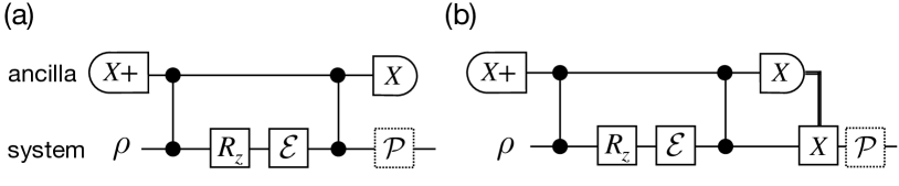
Next, let us consider crafting the remnant error to be biased. In particular, we focus on the Pauli Z rotation gate and aim to bias the error to be XY error, since it can be detected using a single ancilla qubit with less sampling overhead than the lower bound for QEM methods that does not rely on mid-circuit measurement (concrete circuit structure provided in Fig. 3). While we have not found a guaranteed set of shift unitary as in the case for the depolarizing noise, we employ a general strategy of expanding the size of basis set until the synthesis is successful, i.e., the contribution of Z error is below a fixed threshold value (see Supplementary Note S2)

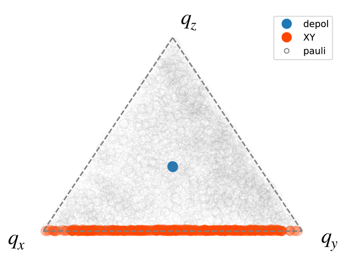
The success of error crafting is highlighted in Fig. 2. As can be seen from Fig. 2(a), while the rate of Pauli errors $(\frac{p_{x}}{p},\frac{p_{y}}{p},\frac{p_{z}}{p})$ is distributed quite homogeneously if we do not impose any constraint on the error profile, the constraints can be reflected with high accuracy. We verify that $p_{x}=p_{y}=p_{z}$ is satisfied up to order of machine precision for the depolarizing constraint, while for the XY-biased noise, we find that we cannot completely eliminate the Z error; there is a small residual component of $p_{z}=O(\epsilon^{3}).$

Refer to caption
Figure 3: Circuit structure for (a) error detection and (b) logical error correction for Pauli Z rotation gate $R_{z}$ with remnant error of $\mathcal{E}_{\rm rem}$. We may further combine with the PEC method, for which the Pauli operation $\mathcal{P}$ with dotted square is executed virtually via updating the Pauli frame. Note that the feedback operation in (b) is also done via Pauli frame.
Gate Synthesis Remnant error QEM method Sampling overhead Novelty Comment
magnitude type
SU(2) Unitary $\epsilon$ coherent PEC $1+4\epsilon$
SU(2) Unitary $\epsilon$ coherent Rescaling $1+2\epsilon^{2}$ Slow WN convergence
SU(2) Crafted $\epsilon^{2}$ Pauli/depol PEC $1+4\epsilon^{2}$
SU(2) Crafted $\epsilon^{2}$ Pauli/depol Rescaling $1+2\epsilon^{2}$
$R_{z}$ Unitary $\epsilon$ coherent PEC $1+4\epsilon$
$R_{z}$ Unitary $\epsilon$ coherent Rescaling $1+2\epsilon^{2}$ Slow WN convergence
$R_{z}$ Crafted $\epsilon^{2}$ Pauli/depol/XY PEC $1+4\epsilon^{2}$
$R_{z}$ Crafted $\epsilon^{2}$ Pauli/depol/XY ED + PEC $1+(q_{x}+q_{y}+4q_{z})\epsilon^{2}$ $q_{z}\sim\epsilon$ in numerics
$R_{z}$ Crafted $\epsilon^{2}$ Pauli/depol/XY ED + Resc. $1+(q_{x}+q_{y}+2q_{z})\epsilon^{2}$ $q_{z}\sim\epsilon$ in numerics
$R_{z}$ Crafted* $\epsilon^{3}$ Pauli Z PEC $1+4\epsilon^{3}$
$R_{z}$ Crafted* $\epsilon^{3}$ Pauli Z Rescaling $1+2\epsilon^{3}$
Table 1: Sampling overhead of error countermeasures under synthesis error of $\epsilon$. The remnant error indicates the diamond distance $d(\mathcal{E}_{\rm rem},\mathcal{I})$ where $\mathcal{I}$ is the identity channel. We assume that unitary gate synthesis is done with accuracy of $\epsilon$, and compare the performance when we further perform probabilistic or error-crafted synthesis. The sampling overhead $\gamma$ is indicated for a single gate, and the total overhead is multiplicative as $\prod_{l}\gamma_{l}$ when overhead is $\gamma_{l}$ for the $l$-th gate. The rescaling technique assumes that the underlying quantum circuit is sufficiently deep so that the white noise (WN) approximation holds. We assume that the white noise approximation holds when rescaling technique is applied. The cubic suppression in the last two rows are verified numerically up to $\epsilon^{3}=10^{-9}$ as shown in Fig. 4. Note that * for the last two rows indicate that synthesis is accompanied with a single ancilla qubit.
Refer to caption
Figure 4: Trade-off between T-count and synthesis accuracy for Pauli rotation gates. We assume that each T gate is subject to depolarizing error of rate $p=10^{-10}$ while Clifford gates are noiseless. The red, yellow, and blue regions indicate the achievable accuracy without any sampling overhead when we employ unitary, probabilistic, and error-crafted synthesis. The blue circuits are the results obtained for $R_{z}(\theta)$ with $\theta\in\{\frac{m\pi}{32}\}_{m\neq 0~{}{\rm mod4}}$ under various synthesis accuracy. The dotted red, yellow, and green lines are given by the empirical T count of $3\log_{2}(1/\varepsilon)$, $1.5\log_{2}(1/\varepsilon)$, and $\log_{2}(1/\varepsilon)$. The chained black line is given by the accumulation of incoherent noise in the T gates.

Even if the Z error cannot be eliminated completely, such an error crafting drastically alters the sampling overhead. By performing the error detection operation as shown in Fig. 3(a), we can mitigate Pauli X and Y errors with sampling overhead of $\gamma_{\rm XY}=1+p_{x}+p_{y},$ which is even below the lower bound of QEM sampling overhead that does not rely on mid-circuit measurement [33]. While the Z error is undetectable and hence we shall rely on other QEM methods such as PEC or rescaling with overhead of $\gamma_{Z}=1+\alpha p_{z}$, the total sampling overhead is $\gamma_{\rm tot}=\gamma_{\rm XY}\gamma_{Z}\sim 1+p_{x}+p_{y}+\alpha p_{z}\sim 1+\epsilon^{2}$. When we perform QEM for $L$ gates, the total sampling overhead $\gamma_{\rm tot}^{L}$ is quartically small compared to that of PEC.

Error crafting using CPTP maps

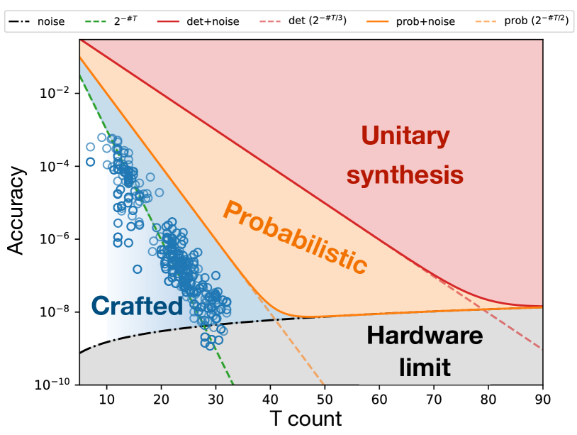
While we have considered the error crafting using synthesized unitaries $\{U_{j}\}$, we can also apply the framework to CPTP maps. As a demonstration, here we consider the target unitary $\hat{U}$ to be a Pauli Z rotation, and constitute the set of implementable CPTPs $\Lambda_{j}$ as the synthesized unitary accompanied with entangled measurement and feedback as shown in Fig. 3(b). By performing brute-force search of $\{\Lambda_{j}\},$ we find that the remnant error can be suppressed cubically small as $\epsilon^{3}$, as opposed to the quadratic suppression realized in the error crafting for unitaries. As we show in Fig. 4, this allows us to synthesize a Pauli rotation gate with T count of $\log_{2}(1/\varepsilon)$ on average, up to accuracy of $\varepsilon=10^{-9}.$ We guide the readers to the Supplementary Note S3S4 for detailed discussion on the search for appropriate $\Lambda_{j}$.

Let us briefly comment on the classical precomputation time of crafted synthesis. Our results in Fig. 4 exploits the direct search algorithm for SU(2) gate synthesis whose computational complexity scales as $O((1/\epsilon))$ on average [51]. Considering that currently known unitary synthesis algorithms for $R_{z}$ gates based on number-theoretic approach [54, 42] or repeat-until-success circuits [46, 39] yield nearly optimal gate sequence with T count of $O({\rm polylog}(1/\epsilon))$, the scaling of direct search algorithms seems to be a significant overhead. Meanwhile, we observe that the actual computation time per synthesis is observed to be milliseconds for the accuracy regime we have investigated. Considering that such computations can be embarrassingly parallelized, and also that number of rotation gates for early FTQC circuits is of $10^{4}$ for quantum dynamics simulation [55, 30] and $10^{6}$ for ground state energy simulation [56], we envision that classical computation time is not bottleneck for such applications.

Last but not least, while we have exclusively discussed the error and sampling overhead only for the synthesis error, it must be kept in mind that, in reality, there is also incoherent noise that indirectly limits the synthesis accuracy. As can be seen from Fig. 4, one shall aim for the sweet-spot where the total error is minimized. While we have displayed the case when we have designed the FTQC to contribute the majority of logical error to magic state distillation, we may flexibly change the scheme to introduce errors in Clifford operations as well.

Summary and outlook

In this work, we have proposed the scheme of error-crafted synthesis of single-qubit unitaries under the framework of Clifford+T formalism. We have proven that we can guarantee the quadratic suppression of the unitary synthesis error even when we constrain the remnant error to be Pauli and depolarizing channel. Furthermore, for the case of Pauli rotation gates, we have numerically shown that error crafting can yield biased Pauli noise such that sampling overhead to mitigate the errors can be suppressed quadratically compared to the existing techniques. We have also found that error crafting for CPTP maps that incorporate measurement and feedback operations achieves cubic suppression of the error up to accuracy of $10^{-9}.$

Numerous future directions are envisioned. First, it is essential to seek whether the error crafting is possible for synthesis of multiqubit unitaries. Combined with the fact that the error can potentially be suppressed exponentially smaller with the qubit count for multiqubit case [41], it is crucial to extend the framework proposed in this work to perform practical quantum computation. Second, it is intriguing in terms of resource theoretic argument to assess the probabilistic transformability between channels. While this has been studied for state transformation in the context of magic state or entanglement distillation [57], the argument on quantum channels is left as an interesting open question. Third, it is an intriguing open question whether there is lower bound on the computational complexity to perform error-crafted synthesis.

Acknowledgement

We thank fruitful discussions with Suguru Endo, Yuuki Tokunaga, and Kunal Sharma. This work was supported by JST CREST Grant Number JPMJCR23I4, JST Moonshot R&D Grant Number JPMJMS2061, MEXT Q-LEAP Grant No. JPMXS0120319794, and No. JPMXS0118068682. N.Y. wishes to thank JST PRESTO No. JPMJPR2119, JST ERATO Grant Number JPMJER2302, JST Grant Number JPMJPF2221, and the support from IBM Quantum. S.A. is supported by JST, PRESTO Grant no.JPMJPR2111. This work is supported by MEXT Quantum Leap Flagship Program (MEXT Q-LEAP) Grant No. JP- MXS0118067394 and JPMXS0120319794, JST COI- NEXT Grant No. JPMJPF2014. K.T. is supported by World-leading Innovative Graduate Study Program for Materials Research, Information, and Technology (MERIT-WINGS) of the University of Tokyo and JSPS KAKENHI Grant No. JP24KJ0857.

References

  • Shor [1995] P. W. Shor, Scheme for reducing decoherence in quantum computer memory, Phys. Rev. A 52, R2493 (1995).
  • Gottesman [1997] D. Gottesman, Stabilizer codes and quantum error correction, arXiv preprint quant-ph/9705052  (1997).
  • Shor [1999] P. W. Shor, Polynomial-time algorithms for prime factorization and discrete logarithms on a quantum computer, SIAM review 41, 303 (1999).
  • Abrams and Lloyd [1999] D. S. Abrams and S. Lloyd, Quantum algorithm providing exponential speed increase for finding eigenvalues and eigenvectors, Phys. Rev. Lett. 83, 5162 (1999).
  • Aspuru-Guzik et al. [2005] A. Aspuru-Guzik, A. D. Dutoi, P. J. Love, and M. Head-Gordon, Simulated quantum computation of molecular energies, Science 309, 1704 (2005).
  • Biamonte et al. [2017] J. Biamonte, P. Wittek, N. Pancotti, P. Rebentrost, N. Wiebe, and S. Lloyd, Quantum machine learning, Nature 549, 195 (2017).
  • Sundaresan et al. [2023] N. Sundaresan, T. J. Yoder, Y. Kim, M. Li, E. H. Chen, G. Harper, T. Thorbeck, A. W. Cross, A. D. Córcoles, and M. Takita, Demonstrating multi-round subsystem quantum error correction using matching and maximum likelihood decoders, Nature Communications 14, 2852 (2023), publisher: Nature Publishing Group.
  • Egan et al. [2021] L. Egan, D. M. Debroy, C. Noel, A. Risinger, D. Zhu, D. Biswas, M. Newman, M. Li, K. R. Brown, M. Cetina, and C. Monroe, Fault-tolerant control of an error-corrected qubit, Nature 598, 281 (2021), publisher: Nature Publishing Group.
  • Ryan-Anderson et al. [2021] C. Ryan-Anderson, J. G. Bohnet, K. Lee, D. Gresh, A. Hankin, J. P. Gaebler, D. Francois, A. Chernoguzov, D. Lucchetti, N. C. Brown, T. M. Gatterman, S. Halit, K. Gilmore, J. Gerber, B. Neyenhuis, D. Hayes, and R. Stutz, Realization of Real-Time Fault-Tolerant Quantum Error Correction, Physical Review X 11, 041058 (2021), publisher: American Physical Society.
  • Bluvstein et al. [2024] D. Bluvstein, S. J. Evered, A. A. Geim, S. H. Li, H. Zhou, T. Manovitz, S. Ebadi, M. Cain, M. Kalinowski, D. Hangleiter, J. P. Bonilla Ataides, N. Maskara, I. Cong, X. Gao, P. Sales Rodriguez, T. Karolyshyn, G. Semeghini, M. J. Gullans, M. Greiner, V. Vuletić, and M. D. Lukin, Logical quantum processor based on reconfigurable atom arrays, Nature 626, 58 (2024), publisher: Nature Publishing Group.
  • Livingston et al. [2022] W. P. Livingston, M. S. Blok, E. Flurin, J. Dressel, A. N. Jordan, and I. Siddiqi, Experimental demonstration of continuous quantum error correction, Nature Communications 13, 2307 (2022), publisher: Nature Publishing Group.
  • Satzinger et al. [2021] K. J. Satzinger, Y. Liu, A. Smith, C. Knapp, M. Newman, C. Jones, Z. Chen, C. Quintana, X. Mi, A. Dunsworth, C. Gidney, I. Aleiner, F. Arute, K. Arya, J. Atalaya, R. Babbush, J. C. Bardin, R. Barends, J. Basso, A. Bengtsson, A. Bilmes, M. Broughton, B. B. Buckley, D. A. Buell, B. Burkett, N. Bushnell, B. Chiaro, R. Collins, W. Courtney, S. Demura, A. R. Derk, D. Eppens, C. Erickson, E. Farhi, L. Foaro, A. G. Fowler, B. Foxen, M. Giustina, A. Greene, J. A. Gross, M. P. Harrigan, S. D. Harrington, J. Hilton, S. Hong, T. Huang, W. J. Huggins, L. B. Ioffe, S. V. Isakov, E. Jeffrey, Z. Jiang, D. Kafri, K. Kechedzhi, T. Khattar, S. Kim, P. V. Klimov, A. N. Korotkov, F. Kostritsa, D. Landhuis, P. Laptev, A. Locharla, E. Lucero, O. Martin, J. R. McClean, M. McEwen, K. C. Miao, M. Mohseni, S. Montazeri, W. Mruczkiewicz, J. Mutus, O. Naaman, M. Neeley, C. Neill, M. Y. Niu, T. E. O’Brien, A. Opremcak, B. Pató, A. Petukhov, N. C. Rubin, D. Sank, V. Shvarts, D. Strain, M. Szalay, B. Villalonga, T. C. White, Z. Yao, P. Yeh, J. Yoo, A. Zalcman, H. Neven, S. Boixo, A. Megrant, Y. Chen, J. Kelly, V. Smelyanskiy, A. Kitaev, M. Knap, F. Pollmann, and P. Roushan, Realizing topologically ordered states on a quantum processor (2021).
  • Bluvstein et al. [2022] D. Bluvstein, H. Levine, G. Semeghini, T. T. Wang, S. Ebadi, M. Kalinowski, A. Keesling, N. Maskara, H. Pichler, M. Greiner, V. Vuletić, and M. D. Lukin, A quantum processor based on coherent transport of entangled atom arrays, Nature 604, 451 (2022), publisher: Nature Publishing Group.
  • Zhao et al. [2022] Y. Zhao, Y. Ye, H.-L. Huang, Y. Zhang, D. Wu, H. Guan, Q. Zhu, Z. Wei, T. He, S. Cao, F. Chen, T.-H. Chung, H. Deng, D. Fan, M. Gong, C. Guo, S. Guo, L. Han, N. Li, S. Li, Y. Li, F. Liang, J. Lin, H. Qian, H. Rong, H. Su, L. Sun, S. Wang, Y. Wu, Y. Xu, C. Ying, J. Yu, C. Zha, K. Zhang, Y.-H. Huo, C.-Y. Lu, C.-Z. Peng, X. Zhu, and J.-W. Pan, Realization of an Error-Correcting Surface Code with Superconducting Qubits, Physical Review Letters 129, 030501 (2022), publisher: American Physical Society.
  • Acharya et al. [2023] R. Acharya, I. Aleiner, R. Allen, T. I. Andersen, M. Ansmann, F. Arute, K. Arya, A. Asfaw, J. Atalaya, R. Babbush, D. Bacon, J. C. Bardin, J. Basso, A. Bengtsson, S. Boixo, G. Bortoli, A. Bourassa, J. Bovaird, L. Brill, M. Broughton, B. B. Buckley, D. A. Buell, T. Burger, B. Burkett, N. Bushnell, Y. Chen, Z. Chen, B. Chiaro, J. Cogan, R. Collins, P. Conner, W. Courtney, A. L. Crook, B. Curtin, D. M. Debroy, A. Del Toro Barba, S. Demura, A. Dunsworth, D. Eppens, C. Erickson, L. Faoro, E. Farhi, R. Fatemi, L. Flores Burgos, E. Forati, A. G. Fowler, B. Foxen, W. Giang, C. Gidney, D. Gilboa, M. Giustina, A. Grajales Dau, J. A. Gross, S. Habegger, M. C. Hamilton, M. P. Harrigan, S. D. Harrington, O. Higgott, J. Hilton, M. Hoffmann, S. Hong, T. Huang, A. Huff, W. J. Huggins, L. B. Ioffe, S. V. Isakov, J. Iveland, E. Jeffrey, Z. Jiang, C. Jones, P. Juhas, D. Kafri, K. Kechedzhi, J. Kelly, T. Khattar, M. Khezri, M. Kieferová, S. Kim, A. Kitaev, P. V. Klimov, A. R. Klots, A. N. Korotkov, F. Kostritsa, J. M. Kreikebaum, D. Landhuis, P. Laptev, K.-M. Lau, L. Laws, J. Lee, K. Lee, B. J. Lester, A. Lill, W. Liu, A. Locharla, E. Lucero, F. D. Malone, J. Marshall, O. Martin, J. R. McClean, T. McCourt, M. McEwen, A. Megrant, B. Meurer Costa, X. Mi, K. C. Miao, M. Mohseni, S. Montazeri, A. Morvan, E. Mount, W. Mruczkiewicz, O. Naaman, M. Neeley, C. Neill, A. Nersisyan, H. Neven, M. Newman, J. H. Ng, A. Nguyen, M. Nguyen, M. Y. Niu, T. E. O’Brien, A. Opremcak, J. Platt, A. Petukhov, R. Potter, L. P. Pryadko, C. Quintana, P. Roushan, N. C. Rubin, N. Saei, D. Sank, K. Sankaragomathi, K. J. Satzinger, H. F. Schurkus, C. Schuster, M. J. Shearn, A. Shorter, V. Shvarts, J. Skruzny, V. Smelyanskiy, W. C. Smith, G. Sterling, D. Strain, M. Szalay, A. Torres, G. Vidal, B. Villalonga, C. Vollgraff Heidweiller, T. White, C. Xing, Z. J. Yao, P. Yeh, J. Yoo, G. Young, A. Zalcman, Y. Zhang, N. Zhu, and Google Quantum AI, Suppressing quantum errors by scaling a surface code logical qubit, Nature 614, 676 (2023), publisher: Nature Publishing Group.
  • Temme et al. [2017] K. Temme, S. Bravyi, and J. M. Gambetta, Error mitigation for short-depth quantum circuits, Phys. Rev. Lett. 119, 180509 (2017).
  • Li and Benjamin [2017] Y. Li and S. C. Benjamin, Efficient variational quantum simulator incorporating active error minimization, Phys. Rev. X 7, 021050 (2017).
  • Endo et al. [2018] S. Endo, S. C. Benjamin, and Y. Li, Practical quantum error mitigation for near-future applications, Phys. Rev. X 8, 031027 (2018).
  • Koczor [2021a] B. Koczor, Exponential error suppression for near-term quantum devices, Phys. Rev. X 11, 031057 (2021a).
  • Huggins et al. [2021] W. J. Huggins, S. McArdle, T. E. O’Brien, J. Lee, N. C. Rubin, S. Boixo, K. B. Whaley, R. Babbush, and J. R. McClean, Virtual distillation for quantum error mitigation, Phys. Rev. X 11, 041036 (2021).
  • Yoshioka et al. [2022] N. Yoshioka, H. Hakoshima, Y. Matsuzaki, Y. Tokunaga, Y. Suzuki, and S. Endo, Generalized quantum subspace expansion, Phys. Rev. Lett. 129, 020502 (2022).
  • van den Berg et al. [2022] E. van den Berg, Z. K. Minev, and K. Temme, Model-free readout-error mitigation for quantum expectation values, Phys. Rev. A 105, 032620 (2022).
  • Strikis et al. [2021] A. Strikis, D. Qin, Y. Chen, S. C. Benjamin, and Y. Li, Learning-based quantum error mitigation, PRX Quantum 2, 040330 (2021).
  • Piveteau et al. [2021] C. Piveteau, D. Sutter, S. Bravyi, J. M. Gambetta, and K. Temme, Error mitigation for universal gates on encoded qubits, Phys. Rev. Lett. 127, 200505 (2021).
  • Suzuki et al. [2022] Y. Suzuki, S. Endo, K. Fujii, and Y. Tokunaga, Quantum error mitigation as a universal error reduction technique: Applications from the nisq to the fault-tolerant quantum computing eras, PRX Quantum 3, 010345 (2022).
  • Yoshioka et al. [2024] N. Yoshioka, T. Okubo, Y. Suzuki, Y. Koizumi, and W. Mizukami, Hunting for quantum-classical crossover in condensed matter problems, npj Quantum Information 10, 45 (2024).
  • Babbush et al. [2018] R. Babbush, C. Gidney, D. W. Berry, N. Wiebe, J. McClean, A. Paler, A. Fowler, and H. Neven, Encoding electronic spectra in quantum circuits with linear t complexity, Phys. Rev. X 8, 041015 (2018).
  • Lee et al. [2021] J. Lee, D. W. Berry, C. Gidney, W. J. Huggins, J. R. McClean, N. Wiebe, and R. Babbush, Even more efficient quantum computations of chemistry through tensor hypercontraction, PRX Quantum 2, 030305 (2021).
  • Sakamoto et al. [2023] K. Sakamoto, H. Morisaki, J. Haruna, E. Itou, K. Fujii, and K. Mitarai, End-to-end complexity for simulating the schwinger model on quantum computers, arXiv preprint arXiv:2311.17388  (2023).
  • Beverland et al. [2022] M. E. Beverland, P. Murali, M. Troyer, K. M. Svore, T. Hoefler, V. Kliuchnikov, G. H. Low, M. Soeken, A. Sundaram, and A. Vaschillo, Assessing requirements to scale to practical quantum advantage, arXiv preprint arXiv:2211.07629  (2022).
  • Eastin and Knill [2009] B. Eastin and E. Knill, Restrictions on transversal encoded quantum gate sets, Phys. Rev. Lett. 102, 110502 (2009).
  • Aharonov et al. [1996] D. Aharonov, M. Ben-Or, R. Impagliazzo, and N. Nisan, Limitations of Noisy Reversible Computation (1996), arXiv:quant-ph/9611028.
  • Tsubouchi et al. [2023] K. Tsubouchi, T. Sagawa, and N. Yoshioka, Universal Cost Bound of Quantum Error Mitigation Based on Quantum Estimation Theory, Physical Review Letters 131, 210601 (2023), publisher: American Physical Society.
  • Takagi et al. [2023] R. Takagi, H. Tajima, and M. Gu, Universal sampling lower bounds for quantum error mitigation, Phys. Rev. Lett. 131, 210602 (2023).
  • Quek et al. [2022] Y. Quek, D. S. França, S. Khatri, J. J. Meyer, and J. Eisert, Exponentially tighter bounds on limitations of quantum error mitigation, arXiv preprint arXiv:2210.11505  (2022).
  • Hastings [2017] M. B. Hastings, Turning gate synthesis errors into incoherent errors, Quantum Info. Comput. 17, 488–494 (2017).
  • Campbell [2017] E. Campbell, Shorter gate sequences for quantum computing by mixing unitaries, Phys. Rev. A 95, 042306 (2017).
  • Wallman and Emerson [2016] J. J. Wallman and J. Emerson, Noise tailoring for scalable quantum computation via randomized compiling, Physical Review A 94, 052325 (2016).
  • Kliuchnikov et al. [2023] V. Kliuchnikov, K. Lauter, R. Minko, A. Paetznick, and C. Petit, Shorter quantum circuits via single-qubit gate approximation, Quantum 7, 1208 (2023).
  • Akibue et al. [2023] S. Akibue, G. Kato, and S. Tani, Probabilistic unitary synthesis with optimal accuracy, arXiv preprint arXiv:2301.06307  (2023).
  • Akibue et al. [2024] S. Akibue, G. Kato, and S. Tani, Probabilistic state synthesis based on optimal convex approximation, npj Quantum Information 10, 1 (2024), publisher: Nature Publishing Group.
  • Ross and Selinger [2016] N. J. Ross and P. Selinger, Optimal ancilla-free clifford+t approximation of z-rotations, Quantum Info. Comput. 16, 901–953 (2016).
  • Fowler [2011] A. G. Fowler, Constructing arbitrary steane code single logical qubit fault-tolerant gates, Quantum Info. Comput. 11, 867–873 (2011).
  • Bocharov and Svore [2012] A. Bocharov and K. M. Svore, Resource-optimal single-qubit quantum circuits, Phys. Rev. Lett. 109, 190501 (2012).
  • Kliuchnikov et al. [2013] V. Kliuchnikov, D. Maslov, and M. Mosca, Fast and efficient exact synthesis of single-qubit unitaries generated by clifford and t gates, Quantum Info. Comput. 13, 607–630 (2013).
  • Bocharov et al. [2015] A. Bocharov, M. Roetteler, and K. M. Svore, Efficient synthesis of universal repeat-until-success quantum circuits, Phys. Rev. Lett. 114, 080502 (2015).
  • van den Berg et al. [2023] E. van den Berg, Z. K. Minev, A. Kandala, and K. Temme, Probabilistic error cancellation with sparse Pauli–Lindblad models on noisy quantum processors, Nature Physics 19, 1116 (2023), publisher: Nature Publishing Group.
  • Takagi [2021] R. Takagi, Optimal resource cost for error mitigation, Phys. Rev. Res. 3, 033178 (2021).
  • Arute et al. [2019] F. Arute, K. Arya, R. Babbush, D. Bacon, J. C. Bardin, R. Barends, R. Biswas, S. Boixo, F. G. S. L. Brandao, D. A. Buell, B. Burkett, Y. Chen, Z. Chen, B. Chiaro, R. Collins, W. Courtney, A. Dunsworth, E. Farhi, B. Foxen, A. Fowler, C. Gidney, M. Giustina, R. Graff, K. Guerin, S. Habegger, M. P. Harrigan, M. J. Hartmann, A. Ho, M. Hoffmann, T. Huang, T. S. Humble, S. V. Isakov, E. Jeffrey, Z. Jiang, D. Kafri, K. Kechedzhi, J. Kelly, P. V. Klimov, S. Knysh, A. Korotkov, F. Kostritsa, D. Landhuis, M. Lindmark, E. Lucero, D. Lyakh, S. Mandrà, J. R. McClean, M. McEwen, A. Megrant, X. Mi, K. Michielsen, M. Mohseni, J. Mutus, O. Naaman, M. Neeley, C. Neill, M. Y. Niu, E. Ostby, A. Petukhov, J. C. Platt, C. Quintana, E. G. Rieffel, P. Roushan, N. C. Rubin, D. Sank, K. J. Satzinger, V. Smelyanskiy, K. J. Sung, M. D. Trevithick, A. Vainsencher, B. Villalonga, T. White, Z. J. Yao, P. Yeh, A. Zalcman, H. Neven, and J. M. Martinis, Quantum supremacy using a programmable superconducting processor, Nature 574, 505 (2019).
  • Dalzell et al. [2024] A. M. Dalzell, N. Hunter-Jones, and F. G. Brandão, Random quantum circuits transform local noise into global white noise, Communications in Mathematical Physics 405, 78 (2024).
  • Morisaki et al. [2024] H. Morisaki, S. Akibue, and K. Fujii, Optimal ancilla-free clifford+t compilation of single qubit unitary, in preparation  (2024).
  • Koczor [2021b] B. Koczor, The dominant eigenvector of a noisy quantum state, New Journal of Physics 23, 123047 (2021b).
  • Cai et al. [2023] Z. Cai, R. Babbush, S. C. Benjamin, S. Endo, W. J. Huggins, Y. Li, J. R. McClean, and T. E. O’Brien, Quantum error mitigation, Rev. Mod. Phys. 95, 045005 (2023).
  • Kliuchnikov et al. [2015] V. Kliuchnikov, D. Maslov, and M. Mosca, Practical approximation of single-qubit unitaries by single-qubit quantum clifford and t circuits, IEEE Transactions on Computers 65, 161 (2015).
  • Campbell [2021] E. T. Campbell, Early fault-tolerant simulations of the hubbard model, Quantum Science and Technology 7, 015007 (2021).
  • Kivlichan et al. [2020] I. D. Kivlichan, C. Gidney, D. W. Berry, N. Wiebe, J. McClean, W. Sun, Z. Jiang, N. Rubin, A. Fowler, A. Aspuru-Guzik, et al., Improved fault-tolerant quantum simulation of condensed-phase correlated electrons via trotterization, Quantum 4, 296 (2020).
  • Regula [2022] B. Regula, Probabilistic transformations of quantum resources, Phys. Rev. Lett. 128, 110505 (2022).
  • Watrous [2009] J. Watrous, Semidefinite programs for completely bounded norms, arXiv preprint arXiv:0901.4709  (2009).
  • Watrous [2012] J. Watrous, Simpler semidefinite programs for completely bounded norms, arXiv preprint arXiv:1207.5726  (2012).
  • Deshpande et al. [2022] A. Deshpande, P. Niroula, O. Shtanko, A. V. Gorshkov, B. Fefferman, and M. J. Gullans, Tight bounds on the convergence of noisy random circuits to the uniform distribution, PRX Quantum 3, 040329 (2022).
  • Tsubouchi et al. [2024] K. Tsubouchi, Y. Mitsuhashi, K. Sharma, and N. Yoshioka, Symmetric clifford twirling for cost-optimal error mitigation in early fault-tolerant quantum computing, arXiv:2405.07720  (2024).
  • Odake et al. [2024] T. Odake, P. Taranto, N. Yoshioka, T. Itoko, K. Sharma, A. Mezzacapo, and M. Murao, Robust error accumulation suppression, arXiv preprint arXiv:2401.16884  (2024).

Supplementary Notes for: Error Crafting in Probabilistic Quantum Gate Synthesis

S1 Formalism of probabilistic synthesis under diamond distance

In the main text, we have discussed the probabilistic synthesis that minimizes the diamond distance $d_{\diamond}(\Phi_{1},\Phi_{2})$ between two unitary channels $\Phi_{1}$ and $\Phi_{2}$. Here, we provide the formal definition of the diamond distance, which is related with the diamond norm as $d_{\diamond}(\Phi_{1},\Phi_{2}):=\frac{1}{2}\|\Phi_{1}-\Phi_{2}\|_{\diamond}$ where $\Phi_{1},\Phi_{2}$ are linear maps from $\mathcal{L}(\mathcal{H}_{1})$ to $\mathcal{L}(\mathcal{H}_{2})$ ($(\mathcal{L}(\mathcal{H}_{i}))$ : the entire set of linear map on $\mathcal{H}_{i}$) for an $d$-dimensional Hilbert space $\mathcal{H}(=\mathcal{H}_{1}=\mathcal{H}_{2})$:

$\displaystyle\|\Phi_{1}-\Phi_{2}\|_{\diamond}:=\max_{\rho\in\mathbb{D}(\mathcal{H}_{1}\otimes\mathcal{H}_{2})}\left\|((\Phi_{1}-\Phi_{2})\otimes{\rm Id}_{d})(\rho)\right\|_{1}.$ (S1)

Here, $\|X\|_{1}={\rm Tr}[\sqrt{X^{\dagger}X}]$ denotes the trace norm, ${\rm Id}_{d}$ is an identity channel acting on $d$-dimensional Hilbert space, and $\mathbb{D}(\mathcal{H}_{1}\otimes\mathcal{H}_{2})$ is the set of physical density matrices on $\mathcal{H}_{1}\otimes\mathcal{H}_{2}$. It is known that the diamond norm $\|\Phi\|_{\diamond}$ can be efficiently calculated via semidefinite programming (SDP) for general linear maps as [58, 59]

(S6)

where $\langle P,Q\rangle={\rm Tr}[P^{\dagger}Q]$ is the inner product of operators $P$ and $Q$, $Y_{0},Y_{1}\in\mathcal{L}(\mathcal{H}_{1})\otimes\mathcal{L}(\mathcal{H}_{2})$ are Hermitian matrices, $\|\cdot\|_{\infty}$ is the spectral norm, and $\mathcal{J}(\Phi)$ is the Choi operator of a map $\Phi$ defined as $\mathcal{J}(\Phi):=({\rm Id}_{d}\otimes\Phi)[|\Omega\rangle\langle\Omega|]$ for the maximally entangled state $|\Omega\rangle=\sum_{i}|i\rangle_{\mathcal{H}_{1}}|i\rangle_{\mathcal{H}_{2}}$. By further assuming that $\Phi_{1}$ and $\Phi_{2}$ are completely positive and trace preserving (CPTP) maps, the calculation can be shown to be simplified as follows.

(S11)

Now let us consider probabilistic synthesis of a target CPTP map $\hat{\Upsilon}$ using a set of CPTP implementable maps $\{\Upsilon_{j}\}$ under the following minimization problem:

(S14)

While it seems complicated since the diamond norm is already defined by minimization, it can be shown that we can solve Eq. (S14) via SDP:

Proposition 1.

Let $\hat{\Upsilon}$ and $\{\Upsilon_{j}\}$ be a target CPTP map and a finite set of implementable CPTP maps from $\mathcal{L}(\mathcal{H}_{1})$ to $\mathcal{L}(\mathcal{H}_{2})$, respectively. Then, the distance $\min_{p}\frac{1}{2}\left\|\hat{\Upsilon}-\sum_{j}p_{j}\Upsilon_{j}\right\|_{\diamond}$ and the optimal probability distribution $\{p_{j}\}$ can be computed with the following SDP:

Primal problem Dual problem
maximize: ${\rm Tr}[\mathcal{J}(\hat{\Upsilon})T]-t$ minimize: $w\in\mathbb{R}$
subject to: $0\leq T\leq\rho\otimes{\rm Id}_{\mathcal{H}_{2}}$, subject to: $S\geq 0,S\geq\mathcal{J}\left(\hat{\Upsilon}-\sum_{j}p_{j}\Upsilon_{j}\right)$,
$\rho\in\mathcal{D}(\mathcal{H}_{1})$, $w{\rm Id}_{\mathcal{H}_{1}}\geq{\rm Tr}_{\mathcal{H}_{2}}[S]$,
$\forall j,{\rm Tr}[\mathcal{J}(\Upsilon_{j})T]\leq t$. $\forall p_{j}\geq 0$, $\sum_{j}p_{j}\leq 1$.
(S15)

Note that the strong duality holds in this SDP, i.e., the optimum primal and dual values are equal.

S1.1 Simplification of probabilistic synthesis in single-qubit case

Although SDP is efficient in a sense that there exists a polynomial-time algorithm with respect to the problem matrix size, in practice the runtime grows quite rapidly, and hence it is desirable to simplify the minimization problem. For the single-qubit case, the calculation of diamond distance boils down to that of trace distance between Choi matrices. While one can show $\frac{1}{d}\|\Phi_{1}-\Phi_{2}\|_{\diamond}\leq\frac{1}{d}\|\mathcal{J}(\Phi_{1})-\mathcal{J}(\Phi_{2})\|_{1}\leq\|\Phi_{1}-\Phi_{2}\|_{\diamond}$ for general $d$-dimensional completely positive maps $\Phi_{1}$ and $\Phi_{2}$, for the single-qubit mixed unitary channel case it is known to saturate the lower bound as $\|\Phi_{1}-\Phi_{2}\|_{\diamond}=\|\mathcal{J}(\Phi_{1})-\mathcal{J}(\Phi_{2})\|_{1}/2.$ Therefore, the remnant error of probabilistic synthesis, $\min_{p}\frac{1}{2}\left\|\hat{\Upsilon}-\sum_{j}p_{j}\Upsilon_{j}\right\|_{\diamond}$, can now be computed by the following simpler semidefinite programming problem:

Primal problem Dual problem
maximize: $\frac{1}{2}{\rm Tr}[M\mathcal{J}(\hat{\Upsilon})]-t$ minimize: ${\rm Tr}[Y]$
subject to: $0\leq M\leq\mathbb{I}$, subject to: $Y\geq 0,Y\geq\frac{1}{2}\mathcal{J}(\hat{\Upsilon})-\frac{1}{2}\sum_{j}p_{j}\mathcal{J}(\Upsilon_{j})$,
$\forall j,\frac{1}{2}{\rm Tr}[M\mathcal{J}(\Upsilon_{j})]\leq t$. $\forall j,p_{j}\geq 0$,$\sum_{j}p_{j}\leq 1$.
(S16)

We further find that it is convenient to introduce the notion of magic basis, an orthonormal basis for the Choi representation of single-qubit channels:

$\displaystyle\ket{\Psi_{1}}=\frac{1}{\sqrt{2}}(\ket{00}+\ket{11}),$ $\displaystyle\ket{\Psi_{2}}=\frac{i}{\sqrt{2}}(\ket{00}-\ket{11}),$
$\displaystyle\ket{\Psi_{3}}=\frac{i}{\sqrt{2}}(\ket{01}+\ket{10}),$ $\displaystyle\ket{\Psi_{4}}=\frac{1}{\sqrt{2}}(\ket{01}-\ket{10}).$ (S17)

It can be shown that this relates a single-qubit unitary channel $\mathcal{U}$ to a unit vector $r\in\mathbb{R}^{4}$ as follows,

$$\frac{1}{2}\left[\mathcal{J}(\mathcal{U})\right]_{MB}=rr^{T},$$ (S18)

where $\left([\cdot]_{MB}\right)_{ij}=\langle\Psi_{i}|\cdot|\Psi_{j}\rangle$.

S2 Numerical details on error crafting using unitaries

S2.1 Crafting Pauli channel

As discussed in the main text, the minimization problem regarding error-crafted synthesis of a Pauli channel is formulated via the following constrained minimization problem of a probability distribution $\{p_{j}\}$ given a target unitary channel $\hat{\mathcal{U}}$ and a set of synthesized unitaries $\{\mathcal{U}_{j}\}$ as follows:

$${\rm minimize}\ \frac{1}{2}\left\|\hat{\mathcal{U}}-\sum_{j}p_{j}\mathcal{U}_{j}\right\|_{\diamond}\ \ \ {\rm subject\ to}\ \ \sum_{j}p_{j}\mathcal{U}_{j}\circ\hat{\mathcal{U}}^{-1}(\cdot)=\sum_{a}\chi_{aa}P_{a}\cdot P_{a},\chi_{aa}\geq 0,$$ (S19)

where $P_{a}\in\{{\rm I},{\rm X},{\rm Y},{\rm Z}\}$ is a single-qubit Pauli operator. In a practical sense, an equality constraint tends to yield numerical instability, and therefore we relax the condition for the remnant error $\mathcal{E}_{\rm rem}=(\sum_{j}p_{j}\mathcal{U}_{j})\circ\hat{\mathcal{U}}^{-1}$ to allow a small violation as

$${\rm minimize}\ \frac{1}{2}\left\|\hat{\mathcal{U}}-\sum_{j}p_{j}\mathcal{U}_{j}\right\|_{\diamond}\ \ \ {\rm subject\ to}\ \ \sum_{j}p_{j}\mathcal{U}_{j}\circ\hat{\mathcal{U}}^{-1}(\cdot)=\sum_{ab}\chi_{ab}P_{a}\cdot P_{b},\sum_{a\neq b}|\chi_{ab}|\leq g_{1},$$ (S20)

where $g_{1}$ is a tolerance factor regarding the Pauli error constraint.

When the set $\{\mathcal{U}_{j}\}$ is not appropriately generated, there does not exist any feasible solution for Eq. (S19). While numerical solvers such as Gurobi offers an automated way to relax the equation constraint, via the variable presolve, we find that this precomputation is done too aggressively so that the accuracy of the minimization is quite poor. Instead, in our work, we have done a logarithmic search of $g_{1}$, starting from machine precision of $g_{1}=10^{-16}$. We have defined the error crafting to be successful if we find feasible solution such that (1) $\min\frac{1}{2}\|\hat{\mathcal{U}}-\sum_{j}p_{j}\mathcal{U}_{j}\|_{\diamond}\leq(c+1)^{2}\epsilon^{2},$ and (2) $g_{1}\leq 10^{-12}$ are both satisfied.

We remark that, using the magic basis introduced in Eq. (S18), the minimization problem boils down to a linear programming problem as

$${\rm minimize}\ 1-\sum_{j}p_{j}\left(r^{(j)}_{1}\right)^{2}\ \ \ {\rm subject\ to}\ \ \sum_{j}p_{j}=1,p_{j}\geq 0,$$ (S21)

where $r^{(j)}=(r_{1}^{(j)},r_{2}^{(j)},r_{3}^{(j)},r_{4}^{(j)})^{T}\in\mathbb{R}^{4}$ corresponds to the magic basis representation of $\mathcal{U}_{j}\circ\hat{\mathcal{U}}^{-1}$. We find that accuracy is much enhanced when the minimization (and relaxation) is done under this representation. In practice, we solve Eq. (S21) using LP implemented in Gurobi, and check if the conditions are satisfied.

S2.2 Crafting depolarizing channel

Here, we provide numerical details regarding the error crafting of depolarizing channel. In similar to Sec. S6.1, the minimization problem is defined as

$${\rm minimize}\ \frac{1}{2}\left\|\hat{\mathcal{U}}-\sum_{j}p_{j}\mathcal{U}_{j}\right\|_{\diamond}\ \ \ {\rm subject\ to}\ \ \sum_{a}\chi_{aa}=1,\chi_{\rm XX}=\chi_{\rm YY}=\chi_{\rm ZZ}\geq 0,\chi_{a\neq b}=0,$$ (S22)

where the set of shift unitary $\{\mathcal{V}_{j}^{(c\epsilon)}\}_{j=1}^{9}$ consists of nine elements, in contrast to seven for the Pauli constraint. Again we relax the equality constraints into inequality constraints for the sake of numerical stability. Concretely, we solve the following problem:

$${\rm minimize}\ \frac{1}{2}\left\|\hat{\mathcal{U}}-\sum_{j}p_{j}\mathcal{U}_{j}\right\|_{\diamond}\ \ \ {\rm subject\ to}\ \ \sum_{a}\chi_{a}=1,\max_{a^{\prime}\neq b^{\prime}}\{|\chi_{a^{\prime}a^{\prime}}-\chi_{b^{\prime}b^{\prime}}|\}\leq g_{2},\sum_{a\neq b}|\chi_{a\neq b}|\leq g_{1},$$ (S23)

where $a\in\{{\rm I},{\rm X},{\rm Y},{\rm Z}\}$ and $a^{\prime},b^{\prime}\in\{{\rm X},{\rm Y},{\rm Z}\}.$ We regard the error crafting to be successful if (1) $\min\frac{1}{2}\|\hat{\mathcal{U}}-\sum_{j}p_{j}\mathcal{U}_{j}\|_{\diamond}\leq(c+1)^{2}\epsilon^{2}$, (2) $g_{1}\leq 10^{-12}$, and (3) $g_{2}\leq 0.01(\sum_{a^{\prime}\in\{X,Y,Z\}}\chi_{a^{\prime}a^{\prime}})\sim 0.01\epsilon^{2}$ are all satisfied.

The results of error-crafted synthesis is shown in Fig. S1. We observe the validity of the nine shift unitary from the bounded behavior in Fig. S1(a). As in the case for Pauli constraint, we also observe a boost in the accuracy by expanding the size of the basis set by factor of $R$. From Figs. S1(b), (c), and (d), we further find that both increasing $c$ and $R$ contributes to suppress the failure probability of the error crafting.

Refer to caption
Figure S1: (a) Diamond distance $d_{\diamond}(\hat{\mathcal{U}},\mathcal{U}_{\rm synth})$ between the target single-qubit Haar random unitary $\hat{\mathcal{U}}$ and synthesized channel $\mathcal{U}_{\rm synth}\coloneqq\sum_{j}p_{j}\mathcal{U}_{j}$, with the remnant error constrained to the single-qubit depolarizing channel. The black real line indicates the results from unitary synthesis by the Ross-Selinger algorithm [42], while the filled dots are results from error-crafted synthesis with shift factors of $c=2,3,5,7.$ When we expand the basis set size by factor of $R=3$, shown by unfilled triangles, the effective synthesis error is suppressed below the bound in Eq. (S58) and approaches the value of $\epsilon^{2}$. The shown data are mean over 200 trials. (b) Failure rate of error-crafted synthesis, averaged over 50 trials. (c)(d) Suppression of $p_{\rm fail}$ with shift factor $c$ and $R$. The data is averaged over 10000 and 2000 trials, respectively.
Refer to caption
Figure S2: Measurement and feedback protocol that corrects X error in implementing a Pauli Z rotation.

S3 Numerical details on error crafting using CPTP maps

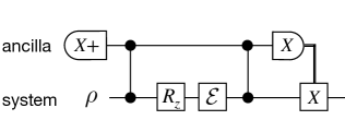
As discussed in the main text, the error of Pauli rotation can be suppressed significantly by applying the error crafting for CPTP maps that represents the channel of synthesized gates accompanied by error correction circuit as shown in Fig. S2. When the target unitary and synthesized unitary channels are given as $\hat{\mathcal{U}}$ and $\mathcal{U}_{j}$, respectively, the effective CPTP channel $\Lambda_{j}$ and remnant error $\mathcal{E}_{{\rm rem},j}$ obtained from logical error correction can be written as

$\displaystyle\Lambda_{j}$ $\displaystyle=$ $\displaystyle\mathscr{T}\left(\mathcal{C}\circ\mathcal{M}_{X}^{(A)}\circ\mathcal{W}_{E}^{\prime}\circ\mathcal{U}_{j}\circ\mathcal{W}_{E}\circ(\Pi_{X+}^{(A)})\right),$ (S24)
$\displaystyle\mathcal{E}_{{\rm rem},j}$ $\displaystyle=$ $\displaystyle\mathscr{T}\left(\mathcal{C}\circ\mathcal{M}_{X}^{(A)}\circ\mathcal{W}_{E}^{\prime}\circ(\mathcal{U}_{j}\circ\hat{\mathcal{U}}^{-1})\circ\mathcal{W}_{E}\circ(\Pi_{X+}^{(A)})\right),$ (S25)

where $\mathscr{T}$ trace outs the ancillary qubit, $\mathcal{C}$ is the correction operation conditioned by the result of the X-measurement on ancilla $\mathcal{M}_{X}^{(A)}$, $\mathcal{W}_{E},\mathcal{W}^{\prime}_{E}$ is the entangling operation between the target and ancilla qubit, and $\Pi_{X+}^{(A)}$ is the state preparation (or force initialization) of $|+\rangle$ state on the ancilla. Note that the expression of Eq. (S25) follows from the fact that $\mathcal{W}_{E}$ and $\mathcal{W}^{\prime}_{E}$ commutes with the target unitary $\hat{\mathcal{U}}.$

In order to clarify how to perform the error crafting for a single-qubit Pauli Z rotation, first note that the Pauli transfer matrix of a remnant error channel $\mathcal{E}_{{\rm rem},j}$ for a Pauli Z rotation, denoted as $\Gamma_{\mathcal{E}_{{\rm rem},j}}$, can be expressed as

$\displaystyle\Gamma_{\mathcal{E}_{{\rm rem},j}}=\begin{pmatrix}1&0&0&0\\ 0&1-\mu_{j}&\nu_{j}&0\\ 0&-\nu_{j}&1-\mu_{j}&0\\ 0&0&0&1\end{pmatrix},$ (S26)

where $0\leq\mu_{j}\leq 1$ and $\Gamma_{\mathcal{E}_{{\rm rem},j}}\geq 0.$ This motivates us to find a pair of remnant error channels $\mathcal{E}_{{\rm rem},+}$ and $\mathcal{E}_{{\rm rem},-}$ which satisfies (i) $\nu_{+}>0,\nu_{-}<0$, (ii) $\mu_{\pm}=O(\epsilon^{3})$. Once such a pair is found, we take the probabilistic mixture of them as

$\displaystyle\tilde{\mathcal{E}}_{\rm rem}$ $\displaystyle=$ $\displaystyle\frac{\nu_{-}}{\nu_{+}+\nu_{-}}\mathcal{E}_{{\rm rem},+}+\frac{\nu_{+}}{\nu_{+}+\nu_{-}}\mathcal{E}_{{\rm rem},-},$ (S27)
$\displaystyle\Gamma_{\tilde{\mathcal{E}}_{\rm rem}}$ $\displaystyle=$ $\displaystyle\begin{pmatrix}1&0&0&0\\ 0&1-\tilde{\mu}&0&0\\ 0&0&1-\tilde{\mu}&0\\ 0&0&0&1\end{pmatrix},$ (S28)

which is a purely Z error channel with error rate of $\tilde{\mu}=\frac{\nu_{-}}{\nu_{+}+\nu_{-}}\mu_{+}+\frac{\nu_{+}}{\nu_{+}+\nu_{-}}\mu_{-}=O(\epsilon^{3}).$

We note that the current search algorithm is based on a brute-force search, and hence the computational complexity is expected to scale as $O({\rm poly}(1/\epsilon))$, while we leave an open question whether there is any bound on complexity to search the pair as in the above discussion. In the current implementation, we generate around 3000 unitaries to reach remnant error of $10^{-6}$ and around 20000 unitaries to reach $10^{-9},$ with each unitary synthesis done in milliseconds using a direct search algorithm proposed in Ref. [51]. Note that each unitary synthesis is independent, and hence is embarrassingly parallelizable.

S4 Generation of shift unitaries with fixed diamond distance

In this section, we discuss how to generate a set of $S$ shift unitaries $\{\mathcal{V}^{\epsilon}_{s}\}_{s=1}^{S}$ which all satisfies $d_{\diamond}(\mathcal{V}_{s}^{\epsilon},\mathcal{I})=\epsilon.$ One of such a method is to generate Haar random unitaries and constrain the “rotation angle” by noting that any single-qubit unitary can be written as $e^{i\theta\sum_{a=X,Y,Z}n_{a}P_{a}}$ where $(n_{X},n_{Y},n_{Z})^{T}\in\mathbb{R}^{3}$ is a unit vector. However, we have found that such a protocol is unsatisfactory in terms of efficiency in generating independent unitaries after unitary synthesis. Therefore, we instead utilize the magic basis representation of a single-qubit unitary. To be precise, given a unit vector $\tilde{v}\in\mathbb{R}^{3},$ we can generate a single-qubit unitary that is expressed in the magic basis representation as

$\displaystyle ee^{T}=\frac{1}{2}\left[\mathcal{J}(\mathcal{U})\right]_{MB}{\rm~{}with~{}}e=\begin{pmatrix}\sqrt{1-\epsilon^{2}}\\ \epsilon\tilde{v}\end{pmatrix}.$ (S29)

Therefore, we may generate unit vectors in order to generate a set of shift unitaries with a fixed value of the diamond distance as follows:

  1. Step 1. Generate a set of unit vectors $\{\tilde{v}_{s}|\tilde{v}_{s}\in\mathbb{R}^{3},\|\tilde{v}_{s}\|_{2}=1\}_{s=1}^{S}$ so that the vectors are distributed on the surface of the sphere as homogeneously as possible.

  2. Step 2. Compute the Choi matrix in the magic basis representation, $\{[\mathcal{J}(\mathcal{V}^{(\epsilon)}_{s})]_{MB}\},$ using the relationship  (S29).

  3. Step 3. Perform basis transformation to obtain $\{\mathcal{J}(\mathcal{V}_{s}^{\epsilon})\}$ in the computational basis, and then compute the matrix representation of shift unitaries $\{V_{s}^{\epsilon}\}$.

In practice, we have employed numerical optimization for Step 1.

S5 White noise approximation under coherent errors

The white noise, or equivalently the global depolarizing noise on $d$-dimensional system acting as $\mathcal{E}_{wn}(\cdot)=(1-p)\cdot+p{\rm Id}/d$ under the rate $p$, is one of the most desirable error profile in the context of estimating expectation values of physical observables. The main reasons are two-fold: $\mathcal{E}_{wn}$ commutes with any gate operations, and it allows unbiased estimation with optimal sampling overhead. All the expectation values of traceless observables shrink homogeneously by a factor of $1-p$ under a single application of $\mathcal{E}_{wn}$, and hence we can unbiasedly estimate the expectation value of an observable $O$ from a noisy estimation as $\expectationvalue*{O}=(1-p)^{-1}\expectationvalue*{O}_{\rm noisy}$. In the case when we have $L$ applications of $\mathcal{E}_{wn}$, we can simply replace $(1-p)^{-1}$ with $(1-p)^{-L}$ and mitigate error with minimal sampling overhead of $(1-p)^{-2L}$.

The white noise has been argued to be realized in experiments, in particular when the unitary gates are chosen at random [49]. In fact, one can prove that, even if the qubit connectivity is only linear and the circuit constitutes a brick-wall structure with random Haar unitary gates for two qubits, the effective noise converges to the white noise under unital noise [50, 60]. However, these arguments mainly consider incoherent error, and how coherent error can affect the white-noise approximation is not fully examined. Given that the coherent component of error arises as the synthesis error in the early FTQC regime, it is crucial to investigate the effect of coherent errors on the white-noise approximation.

Let us assume that one aims to simulate a $n$-qubit layered quantum circuit $\hat{\mathcal{U}}:=\mathcal{U}_{L+1}\circ\mathcal{U}_{L}\circ\cdots\circ\mathcal{U}_{1}$ which is exposed to noise channels as $\mathcal{U}=\mathcal{U}_{L+1}\circ\mathcal{E}\circ\mathcal{U}_{L}\circ\cdots\mathcal{E}\circ\mathcal{U}_{1}.$ We define the effective noise channel $\mathcal{E}^{\prime}$ by re-expressing the noisy layered circuit as $\mathcal{U}=\mathcal{E}^{\prime}\circ\hat{\mathcal{U}}$, When we expect that $\mathcal{E}^{\prime}$ is close to the global white noise, we can mitigate errors and restore the ideal expectation value via some constant factor $R$, namely by rescaling the noisy one as $\mathrm{tr}[\rho O]=R\mathrm{tr}[\mathcal{E}^{\prime}(\rho)O]$. Especially when each unitary layer $\mathcal{U}_{l}(\cdot)=U_{l}\cdot U_{l}^{\dagger}$ is chosen randomly from $n$-qubit Haar random unitary, we can bound the bias between the ideal and the rescaled expectation value as

$\displaystyle\mathbb{E}_{U}\left[\big{|}R\mathrm{tr}[\mathcal{E}^{\prime}(\rho)O]-\mathrm{tr}[\rho O]\big{|}\right]\leq\sqrt{1-\quantity(\frac{s^{2}}{u})^{L}},$ (S30)

by choosing the rescaling factor as $R=(s/u)^{L}$ (Theorem S1 of [61]). Here, $u$ and $s$ are noise-dependent constants called unitarity and average noise strength, respectively, which can be represented as

$\displaystyle u$ $\displaystyle=$ $\displaystyle\frac{\sum_{ij}|\mathrm{tr}[E_{i}E_{j}^{\dagger}]|^{2}-1}{4^{n}-1}$ (S31)
$\displaystyle s$ $\displaystyle=$ $\displaystyle\frac{\sum_{i}|\mathrm{tr}[E_{i}]|^{2}-1}{4^{n}-1},$ (S32)

where $E_{i}$ is the Kraus operators of the noise $\mathcal{E}$.

For incoherent error such as the local depolarizing noise with uniform error rate $\mathcal{E}=\bigcirc_{i=1}^{n}\mathcal{E}^{(i)}_{\mathrm{dep}}$, where $\mathcal{E}^{(i)}_{\mathrm{dep}}(\cdot)=(1-\frac{3}{4}p)\cdot+\frac{p}{4}(X_{i}\cdot X_{i}+Y_{i}\cdot Y_{i}+Z_{i}\cdot Z_{i})$ is the single-qubit local depolarizing channel on the $i$-th qubit, we obtain

$$\mathbb{E}_{U}[|R\mathrm{tr}[\mathcal{E}^{\prime}(\rho)O]-\mathrm{tr}[\rho O]|]\leq O(\sqrt{nL}p)\;\;\text{with}\;\;R=(1+O(p))^{nL}$$ (S33)

from Eq. (S30). Meanwhile, for coherent error $\mathcal{E}=\bigcirc_{i=1}^{n}\mathcal{E}^{(i)}_{\mathrm{coh}}$ with $\|\mathcal{E}_{\rm coh}^{(i)}-{\rm Id}\|_{\diamond}=\epsilon_{\rm coh}$, we obtain

$$\mathbb{E}_{U}[|R\mathrm{tr}[\mathcal{E}^{\prime}(\rho)O]-\mathrm{tr}[\rho O]|]\leq O(\sqrt{nL}\epsilon_{\rm coh})\;\;\text{with}\;\;R=(1+O(\epsilon_{\rm coh}^{2}))^{nL}.$$ (S34)

These results mean that, in terms of the sampling overhead $R^{2}$, coherent errors have quadratically suppressed sampling overhead compared to incoherent errors (see also Table S1). However, its effect on the bias is linear as in the case of incoherent errors. Therefore, it is preferable to suppress its error rate through randomized compiling or error crafting, and improve the performance of the white-noise approximation.

Table S1: Performance of the QEM through rescaling the noisy expectation value assuming the white-noise approximation for incoherent error with error rate $p$ and coherent error with diamond norm $\epsilon_{\rm coh}^{2}$. While coherent errors have quadratically suppressed sampling overhead, their effect on the bias is comparable with incoherent errors.
Error model Bias Sampling overhead
Incoherent error $O(\sqrt{nL}p)$ $(1+O(p))^{2nL}$
Coherent error $O(\sqrt{nL}\epsilon_{\rm coh})$ $(1+O(\epsilon_{\rm coh}^{2}))^{2nL}$

We can observe a similar scaling numerically. Before discussing the effect of the coherent noise, let us briefly summarize the numerical argument for incoherent noise, especially the local depolarizing noise $\mathcal{E}=\bigcirc_{i=1}^{n}\mathcal{E}^{(i)}_{\mathrm{dep}}$, provided in Ref. [33]. We analyze the convergence to white noise by examining the Pauli transfer matrix (PTM) of the effective noise $\mathcal{E}^{\prime}$, denoted hereafter as $\Gamma$. We define $\Gamma$ by $\Gamma_{ij}={\rm Tr}[P_{i}\mathcal{E}^{\prime}(P_{j})]/2^{n}$ for $P_{i},P_{j}\in\{I,X,Y,Z\}^{\otimes n}$ for $n$-qubit system. Note that PTM is diagonal if $\mathcal{E}^{\prime}$ is a Pauli channel, and furthermore there exists $0\leq w\leq 1$ such that $\Gamma_{ii}=w~{}(i\neq 0)$ if $\mathcal{E}^{\prime}$ is the white noise. In this regard, it is useful to compute the singular values of the PTM in order to investigate the closeness to the white noise. We in particular compute $\Gamma=V\Lambda W^{\dagger}$ with $\Lambda={\rm diag}\{\lambda_{i}\}_{i=1}^{4^{n}}$, and define the damping factor $k_{i}$ as follows,

$\displaystyle\lambda_{i}=(1-p)^{-k_{i}L}.$ (S35)

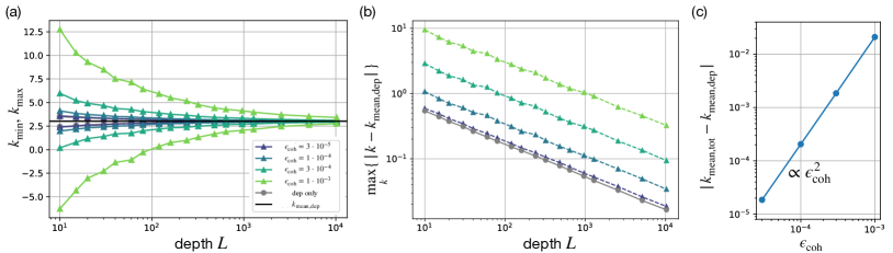
It can be proven that, when each unitary layer consists of unitary 2-design, the damping factor converges to $k_{\rm mean}=\frac{3n}{4}\frac{4^{n}}{4^{n}-1}$, and numerical analysis supports that this also holds for weaker randomness, e.g., 2-local random circuits with linear connectivity, when the circuit depth is sufficiently deep. In other words, the mean deviation $\mathbb{E}_{i}[|k_{i}-k_{\rm mean}|]$, as well as the deviation of extremals $|k_{\rm max(min)}-k_{\rm mean}|$, is suppressed as $O(1/\sqrt{L})$ [33], which is consistent with the suppression of total variation distance in measurement probability distribution in the computational basis [50].

Now we ask how the above behavior is affected by the presense of coherent errors. Here, for the sake of simplicity of the argument, we sample $U_{i}$ uniformly from the entire unitary group, i.e., take an $n$-qubit Haar random unitary, and consider a local noise as $\mathcal{E}_{l}=\bigcirc_{i=1}^{n}\mathcal{E}_{\rm coh}^{(i)}\circ\mathcal{E}_{\rm dep}^{(i)},$ where $\mathcal{E}_{\rm coh}^{(i)}$ is a random 1-qubit unitary such that $\|\mathcal{E}_{\rm coh}^{(i)}-{\rm Id}\|_{\diamond}=\epsilon_{\rm coh}.$ In practice, this can be realized by constraining the rotation angles under axial decomposition of the unitary.

Interestingly, we find that the effect of coherent error on the magnitude of the white noise is quadratically suppressed, while that on the convergence rate is linear. In Fig. S3(a)(b) we can see that, although the fluctuation in the damping factor is expanded at the shallow-depth regime, it readily converges at the rate of $O(1/\sqrt{L})$, which is in similar to the depolarizing-only case [33]. We observe that the deviation $\max_{k}\{|k-k_{\rm mean,dep}|\}$ is lifted approximately by a factor of $(\epsilon_{\rm coh}+\epsilon_{\rm dep})/\epsilon_{\rm dep}$ where $\epsilon_{\rm dep}:=\|\mathcal{E}_{\rm dep}^{(i)}-{\rm Id}\|_{\diamond}$, implying the slow down of the white noise convergence. Meanwhile, as shown in Fig. S3(c), we notice that the converged effective channel is less affected, in a sense that $|k_{\rm mean,tot}-k_{\rm mean,dep}|\propto\epsilon^{2}.$ Phenomenologically, we can understand that the effect of coherent noise is self-twirled by the circuit such that the diamond norm is suppressed quadratically as in the random compilation scheme [62]. These results indicate that, although the presence of coherent error does not severely increase the sampling overhead to perform error countermeasures such as the rescaling technique, the adequacy of the approximation is degraded and hence desirable to avoid them by error-crafted synthesis.

Refer to caption
Figure S3: Convergence to white noise in $n=4$ qubit quantum circuit. (a) Extremal values of damping factors $k_{\rm min}$ and $k_{\rm max}$ at various $L$. The unitary layer is drawn uniform-randomly from the $n$-qubit unitary group. Each layer is subject to error $\bigcirc_{i=1}^{N}\mathcal{E}_{\rm coh}\circ\mathcal{E}_{\rm dep}$ with depolarizing error rate of $p=10^{-4}.$ (b) The largest deviation from $k_{\rm mean,dep},$ the value realized when only the depolarizing noise is present ($\epsilon_{\rm coh}=0$). (c) The quadratic suppression of damping factor $k$ with respect to the contribution from coherent noise. Here, we compute $|k_{\rm mean,tot}-k_{\rm mean,dep}|$ at $L=10^{4}$.

S6 Theoretical guarantees for error crafted synthesis

S6.1 Crafting Pauli channel (Proof of Theorem 1)

In this section, we provide the formal statement and proof for Theorem 1 in the main text. First, we rewrite the Pauli-constrained minimization problem using the magic basis introduced in Sec. S1 to obtain the following,

$${\rm minimize}\ 1-\sum_{j}p_{j}\left(r^{(j)}_{1}\right)^{2}\ \ \ {\rm subject\ to}\ \ \sum_{j}p_{j}r^{(j)}r^{(j)T}\ {\rm is\ diagonal},$$ (S36)

where $r^{(j)}=(r_{1}^{(j)},r_{2}^{(j)},r_{3}^{(j)},r_{4}^{(j)})\in\mathbb{R}^{4}$ corresponds to the magic basis representation of the error channel for the $j$-th basis $\mathcal{U}_{j}\circ\hat{\mathcal{U}}^{-1}$. As we described in Sec. S1, this optimization can be solved by linear programming if the solution exists. Thus, the only nontrivial part for tailoring Pauli error is how to guarantee the existence of a solution. As we already mentioned in the main text, we rigorously guarantee the existence of such a basis set:

Theorem S1.

(Detailed version of Theorem 1.) There exist a positive numbers $c$, $\epsilon_{0}$ and unit vectors $\{\hat{\vec{v}}^{(j)}\in\mathbb{R}^{3}\}_{j=1}^{7}$ such that for any given single-qubit unitary $\hat{\mathcal{U}}$ and for any $\epsilon\in(0,\epsilon_{0}]$, if we construct target unitaries $\{\hat{\mathcal{U}}_{j}\}_{j=1}^{7}$ satisfying

$$\frac{1}{2}\left[\mathcal{J}(\hat{\mathcal{U}}_{j}\circ\hat{\mathcal{U}}^{-1})\right]_{MB}=\hat{e}^{(j)}\hat{e}^{(j)T}\ \ {\rm with}\ \ \hat{e}^{(j)}=\begin{pmatrix}\sqrt{1-(c\epsilon)^{2}}\\ c\epsilon\hat{\vec{v}}^{(j)}\end{pmatrix}$$ (S37)

and obtain $\{\mathcal{U}_{j}\}_{j}$ via unitary synthesis such that $\frac{1}{2}\left\|\hat{\mathcal{U}}_{j}-\mathcal{U}_{j}\right\|_{\diamond}\leq\epsilon$, then a solution in Eq. (S19) exists. Moreover, it holds that

$$((c-1)\epsilon)^{2}\leq\frac{1}{2}\left\|\hat{\mathcal{U}}-\sum_{j=1}^{7}p_{j}\mathcal{U}_{j}\right\|_{\diamond}\leq((c+1)\epsilon)^{2}$$ (S38)

with the optimal probability distribution $\{p_{j}\}$ that induces a Pauli synthesis error.

Proof.

By letting $r^{(j)}$ be the magic basis representation of $\mathcal{U}_{j}\circ\hat{\mathcal{U}}^{-1}$ and defining

$$A_{L}=\begin{pmatrix}r^{(1)}_{1}r^{(1)}_{2}&r^{(2)}_{1}r^{(2)}_{2}&\cdots&r^{(L)}_{1}r^{(L)}_{2}\\ r^{(1)}_{1}r^{(1)}_{3}&r^{(2)}_{1}r^{(2)}_{3}&\cdots&r^{(L)}_{1}r^{(L)}_{3}\\ r^{(1)}_{1}r^{(1)}_{4}&r^{(2)}_{1}r^{(2)}_{4}&\cdots&r^{(L)}_{1}r^{(L)}_{4}\\ r^{(1)}_{2}r^{(1)}_{3}&r^{(2)}_{2}r^{(2)}_{3}&\cdots&r^{(L)}_{2}r^{(L)}_{3}\\ r^{(1)}_{2}r^{(1)}_{4}&r^{(2)}_{2}r^{(2)}_{4}&\cdots&r^{(L)}_{2}r^{(L)}_{4}\\ r^{(1)}_{3}r^{(1)}_{4}&r^{(2)}_{3}r^{(2)}_{4}&\cdots&r^{(L)}_{3}r^{(L)}_{4}\end{pmatrix}=\begin{pmatrix}m^{(1)}&m^{(2)}&\cdots&m^{(L)}\end{pmatrix},$$ (S39)

we can describe the non-diagonal elements in $\sum_{j=1}^{L}p_{j}r^{(j)}r^{(j)T}$ obtained by mixing $\{\mathcal{U}_{j}\}_{j=1}^{L}$ as a vector $A_{L}p$.

Suppose that $A_{6}$ is invertible. Then, it is sufficient to show $(A_{6}^{-1}m^{(7)})_{i}\leq 0$ for any $i\in\{1,\cdots,6\}$. This is because $\mathbf{e}^{(i)T}A_{6}^{-1}m^{(k)}=\delta_{ik}$, where $\delta_{ik}$ is the Kronecker delta and $\mathbf{e}^{(i)}$ is the unit vector whose element is 00 except the $i$-th element,

$\displaystyle\forall i\in\{1,\cdots,6\},\mathbf{e}^{(i)T}A_{6}^{-1}m^{(7)}\leq 0$ $\displaystyle\Leftrightarrow$ $\displaystyle\exists\tilde{p}:\{1,\cdots,6\}\rightarrow[0,\infty),m^{(7)}=-\sum_{j=1}^{6}\tilde{p}_{j}m^{(j)},$ (S40)

and we can verify $A_{7}p=0$ by setting $p_{j}=\frac{\tilde{p}_{j}}{1+\sum_{j^{\prime}=1}^{6}\tilde{p}_{j^{\prime}}}$ for $j\in\{1,\cdots,6\}$ and $p_{7}=\frac{1}{1+\sum_{j=1}^{6}\tilde{p}_{j}}$.

In the following, we show that $A_{6}$ is invertible and $\max_{i}(A_{6}^{-1}m^{(7)})_{i}\leq 0$ by using the continuity of the matrix inverse. Define $D=diag(\frac{1}{c\epsilon\sqrt{1-(c\epsilon)^{2}}},\frac{1}{c\epsilon\sqrt{1-(c\epsilon)^{2}}},\frac{1}{c\epsilon\sqrt{1-(c\epsilon)^{2}}},\frac{1}{(c\epsilon)^{2}},\frac{1}{(c\epsilon)^{2}},\frac{1}{(c\epsilon)^{2}})$. By letting

$\displaystyle\hat{\vec{v}}^{(1)}=\begin{pmatrix}-1\\ 0\\ 0\end{pmatrix},\hat{\vec{v}}^{(2)}=\begin{pmatrix}0\\ -1\\ 0\end{pmatrix},\hat{\vec{v}}^{(3)}=\begin{pmatrix}0\\ 0\\ 1\end{pmatrix},\hat{\vec{v}}^{(4)}=\frac{1}{\sqrt{2}}\begin{pmatrix}1\\ -1\\ 0\end{pmatrix},\hat{\vec{v}}^{(5)}=\frac{1}{\sqrt{2}}\begin{pmatrix}-1\\ 0\\ -1\end{pmatrix},\hat{\vec{v}}^{(6)}=\frac{1}{\sqrt{2}}\begin{pmatrix}0\\ 1\\ 1\end{pmatrix},\hat{\vec{v}}^{(7)}=\frac{1}{\sqrt{3}}\begin{pmatrix}1\\ 1\\ -1\end{pmatrix},$

we can verify that

$\displaystyle D\hat{A}_{6}=\begin{pmatrix}-1&0&0&\frac{1}{\sqrt{2}}&-\frac{1}{\sqrt{2}}&0\\ 0&-1&0&-\frac{1}{\sqrt{2}}&0&\frac{1}{\sqrt{2}}\\ 0&0&1&0&-\frac{1}{\sqrt{2}}&\frac{1}{\sqrt{2}}\\ 0&0&0&-\frac{1}{2}&0&0\\ 0&0&0&0&\frac{1}{2}&0\\ 0&0&0&0&0&\frac{1}{2}\\ \end{pmatrix},(D\hat{A}_{6})^{-1}=\begin{pmatrix}-1&0&0&-\sqrt{2}&-\sqrt{2}&0\\ 0&-1&0&\sqrt{2}&0&\sqrt{2}\\ 0&0&1&0&\sqrt{2}&-\sqrt{2}\\ 0&0&0&-2&0&0\\ 0&0&0&0&2&0\\ 0&0&0&0&0&2\\ \end{pmatrix},\hat{A}_{6}^{-1}\hat{m}^{(7)}=-\frac{1}{3}\begin{pmatrix}\sqrt{3}\\ \sqrt{3}\\ \sqrt{3}\\ 2\\ 2\\ 2\end{pmatrix},$ (S42)

where $\hat{A}_{6}$ is the matrix defined in the same way as Eq. (S39) for $\hat{\mathcal{U}}_{j}\circ\hat{\mathcal{U}}^{-1}$, and we use $\hat{A}_{6}^{-1}\hat{m}^{(7)}=(D\hat{A}_{6})^{-1}D\hat{m}^{(7)}$ in the last equality. If we can show that there exists an upper bound $u(c,\epsilon)$ of $\left\|Dm^{(j)}-D\hat{m}^{(j)}\right\|_{2}$ satisfying

$$\forall j,\left\|Dm^{(j)}-D\hat{m}^{(j)}\right\|_{2}\leq u(c,\epsilon)\ \ \wedge\ \ \lim_{c\rightarrow\infty}\lim_{\epsilon\rightarrow 0}u(c,\epsilon)=0,$$ (S43)

it implies that $DA_{6}$ is invertible ($\Leftrightarrow$ $A_{6}$ is invertible) and $\max_{i}(A_{6}^{-1}m^{(7)})_{i}=\max_{i}((DA_{6})^{-1}Dm^{(7)})_{i}\leq 0$ for large enough $c$ and small enough $\epsilon$ since $D\hat{A}_{6}$ is a constant invertible matrix (independent to $\epsilon$), $\max_{i}((D\hat{A}_{6})^{-1}D\hat{m}^{(7)})_{i}=-\frac{1}{\sqrt{3}}$, the set of invertible matrices is open, and $f:A\rightarrow A^{-1}$ is continuous.

In the following, we assume that $c>1$ and $\epsilon_{0}<\frac{1}{2c}$ and consider the case when $\epsilon\in(0,\epsilon_{0}]$. Let $\sin\hat{\theta}=c\epsilon$, $\sin\theta_{0}=\epsilon$ and $r^{(j)}=(\cos\theta_{j},\sin\theta_{j}\vec{v}^{(j)})^{T}$ with $\hat{\theta},\theta_{0}\in(0,\pi/6),\theta_{j}\in[0,\pi/2]$. Since the following argument holds for any $j$, we abbreviate a subscript or superscript indicating a label $j$. From the assumption of compilation accuracy, we obtain

$$\cos\theta_{0}=\sqrt{1-\epsilon^{2}}\leq|e\cdot\hat{e}|=|\cos\theta\cos\hat{\theta}+\sin\theta\sin\hat{\theta}\vec{v}\cdot\hat{\vec{v}}|=\cos\theta\cos\hat{\theta}+\sin\theta\sin\hat{\theta}\vec{v}\cdot\hat{\vec{v}},$$ (S44)

where we use $\theta<\frac{\pi}{3}$ (due to $|\theta-\hat{\theta}|<\theta_{0}$) in the last equality. By using $\theta>0$ (due to $c>1$), this is equivalent to

$$|\theta-\hat{\theta}|\leq\theta_{0}\wedge\ \vec{v}\cdot\hat{\vec{v}}\geq\frac{\cos\theta_{0}-\cos\theta\cos\hat{\theta}}{\sin\theta\sin\hat{\theta}}(>0).$$ (S45)

On the other hand,

$\displaystyle\left\|D(m-\hat{m})\right\|_{2}$ $\displaystyle=$ $\displaystyle\sqrt{\left\|\hat{\vec{v}}-\frac{\cos\theta\sin\theta}{\cos\hat{\theta}\sin\hat{\theta}}\vec{v}\right\|_{2}^{2}+\left\|\begin{pmatrix}\hat{v}_{1}\hat{v}_{2}\\ \hat{v}_{1}\hat{v}_{3}\\ \hat{v}_{2}\hat{v}_{3}\end{pmatrix}-\left(\frac{\sin\theta}{\sin\hat{\theta}}\right)^{2}\begin{pmatrix}v_{1}v_{2}\\ v_{1}v_{3}\\ v_{2}v_{3}\end{pmatrix}\right\|_{2}^{2}}$ (S46)
$\displaystyle=$ $\displaystyle\sqrt{\left\|\hat{\vec{v}}-\frac{\sin(2\theta)}{\sin(2\hat{\theta})}\vec{v}\right\|_{2}^{2}+\frac{1}{2}\left(\left\|\hat{\vec{v}}\hat{\vec{v}}^{T}-\left(\frac{\sin\theta}{\sin\hat{\theta}}\right)^{2}\vec{v}\vec{v}^{T}\right\|_{2}^{2}-\sum_{i=1}^{3}\left(\hat{v}_{i}^{2}-\left(\frac{\sin\theta}{\sin\hat{\theta}}\right)^{2}v_{i}^{2}\right)^{2}\right)}$ (S47)
$\displaystyle\leq$ $\displaystyle\sqrt{\left\|\hat{\vec{v}}-\frac{\sin(2\theta)}{\sin(2\hat{\theta})}\vec{v}\right\|_{2}^{2}+\frac{1}{2}\left(\left\|\hat{\vec{v}}\hat{\vec{v}}^{T}-\left(\frac{\sin\theta}{\sin\hat{\theta}}\right)^{2}\vec{v}\vec{v}^{T}\right\|_{2}^{2}-\frac{1}{3}\left(1-\left(\frac{\sin\theta}{\sin\hat{\theta}}\right)^{2}\right)^{2}\right)},$ (S48)

where we use the Cauchy-Schwartz inequality $\left(\sum_{i=1}^{3}\left(\hat{v}_{i}^{2}-\frac{\sin^{2}\theta}{\sin^{2}\hat{\theta}}v_{i}^{2}\right)^{2}\right)\left(\sum_{i=1}^{3}\left(\frac{1}{\sqrt{3}}\right)^{2}\right)\geq\left(\sum_{i=1}^{3}\frac{1}{\sqrt{3}}\left(\hat{v}_{i}^{2}-\frac{\sin^{2}\theta}{\sin^{2}\hat{\theta}}v_{i}^{2}\right)\right)^{2}$ in the last inequality. We proceed the calculation as follows:

Eq.(S48)formulae-sequence𝐸𝑞italic-(S48italic-)\displaystyle Eq.~{}\eqref{eq:dm1} $\displaystyle=$ $\displaystyle\sqrt{1+\left(\frac{\sin(2\theta)}{\sin(2\hat{\theta})}\right)^{2}-2\frac{\sin(2\theta)}{\sin(2\hat{\theta})}\vec{v}\cdot\hat{\vec{v}}+\frac{1}{2}\left(1+\left(\frac{\sin\theta}{\sin\hat{\theta}}\right)^{4}-2\left(\frac{\sin\theta}{\sin\hat{\theta}}\vec{v}\cdot\hat{\vec{v}}\right)^{2}\right)-\frac{1}{6}\left(1-\left(\frac{\sin\theta}{\sin\hat{\theta}}\right)^{2}\right)^{2}}.$

By using Eq. (S45), we obtain

$$\left\|D(m-\hat{m})\right\|_{2}\leq\max_{|\theta-\hat{\theta}|\leq\theta_{0}}\sqrt{f(\hat{\theta},\theta,\theta_{0})}=\sqrt{\max_{|t|\leq 1}f(\hat{\theta},\theta_{0}t+\hat{\theta},\theta_{0})},$$ (S50)

where $f(\hat{\theta},\theta,\theta_{0})=1+\left(\frac{\sin(2\theta)}{\sin(2\hat{\theta})}\right)^{2}-2\frac{\sin(2\theta)}{\sin(2\hat{\theta})}\frac{\cos\theta_{0}-\cos\theta\cos\hat{\theta}}{\sin\theta\sin\hat{\theta}}+\frac{1}{2}\left(1+\left(\frac{\sin\theta}{\sin\hat{\theta}}\right)^{4}-2\left(\frac{\cos\theta_{0}-\cos\theta\cos\hat{\theta}}{\sin^{2}\hat{\theta}}\right)^{2}\right)-\frac{1}{6}\left(1-\left(\frac{\sin\theta}{\sin\hat{\theta}}\right)^{2}\right)^{2}$. Define $g_{c}(\epsilon,t):=f(\sin^{-1}(c\epsilon),\sin^{-1}(\epsilon)t+\sin^{-1}(c\epsilon),\sin^{-1}(\epsilon))$ on $(\epsilon,t)\in(0,\epsilon_{0}]\times[-1,1]$. To complete the proof of Eq. (S43), it is sufficient to show $\lim_{c\rightarrow\infty}\lim_{\epsilon\rightarrow 0}\max_{|t|\leq 1}g_{c}(\epsilon,t)=0$. As shown in Section S7.1, $g_{c}(\epsilon,t)$ is uniformly continuous in $(\epsilon,t)\in(0,\epsilon_{0}]\times[-1,1]$. Thus, we can interchange $\lim_{\epsilon\rightarrow 0}$ and $\max_{|t|\leq 1}$ (see detail in Section S7.2) and obtain

$\displaystyle\lim_{\epsilon\rightarrow 0}\max_{|t|\leq 1}g_{c}(\epsilon,t)$ $\displaystyle=$ $\displaystyle\max_{|t|\leq 1}\lim_{\epsilon\rightarrow 0}g_{c}(\epsilon,t)$ (S51)
$\displaystyle=$ $\displaystyle\max_{|t|\leq 1}\frac{1}{c^{4}}\left(\frac{1}{12}t^{4}+\frac{c}{3}t^{3}+\left(\frac{c^{2}}{3}+\frac{1}{2}\right)t^{2}+ct+2c^{2}-\frac{1}{4}\right)$ (S52)
$\displaystyle=$ $\displaystyle\frac{7}{3c^{2}}+\frac{4}{3c^{3}}+\frac{1}{3c^{4}},$ (S53)

where the last equality is obtained by observing that $t=1$ maximizes the polynomial via a straightforward calculation. Finally, we obtain

$$\left\|Dm-D\hat{m}\right\|_{2}\leq u(c,\epsilon)\ \ \wedge\ \ \lim_{\epsilon\rightarrow 0}u(c,\epsilon)=\sqrt{\frac{7}{3c^{2}}+\frac{4}{3c^{3}}+\frac{1}{3c^{4}}}.$$ (S54)

This completes the proof. ∎

S6.2 Crafting depolarizing channel

In similar to the Pauli constraint, the minimization problem to obtain the synthesis probability distribution under the depolarizing constraint can be written as

$${\rm minimize}\ \frac{1}{2}\left\|\hat{\mathcal{U}}-\sum_{j}p_{j}\mathcal{U}_{j}\right\|_{\diamond}\ \ \ {\rm subject\ to}\ \ \sum_{a}\chi_{aa}=1,\chi_{\rm XX}=\chi_{\rm YY}=\chi_{\rm ZZ}=q\geq 0,\chi_{a\neq b}=0,$$ (S55)

which is rewritten under the magic basis representation as

$${\rm minimize}\ 1-\sum_{j}p_{j}\left(r^{(j)}_{1}\right)^{2}\ \ \ {\rm subject\ to}\ \ \sum_{j}p_{j}r^{(j)}e^{(j)T}=(1-q)\mathbf{e}^{(1)}\mathbf{e}^{(1)T}+\frac{q}{4}{\rm Id},$$ (S56)

where $r^{(j)}\in\mathbb{R}^{4}$ corresponds to the magic basis representation of $\mathcal{U}_{j}\circ\hat{\mathcal{U}}^{-1}$ given in Eq. (S18), and $\mathbf{e}^{(i)}$ is the unit vector whose element is 00 except the $i$-th element.

We can prove the feasibility guarantee as in the following theorem:

Theorem S2.

There exist positive numbers $c$, $\epsilon_{0}$ and unit vectors $\{\hat{\vec{v}}^{(j)}\in\mathbb{R}^{3}\}_{j=1}^{9}$ such that for any given single-qubit unitary $\hat{\mathcal{U}}$ and for any $\epsilon\in(0,\epsilon_{0}]$, if we prepare target unitaries $\{\hat{\mathcal{U}}_{j}\}_{j=1}^{9}$ satisfying

$$\frac{1}{2}\left[\mathcal{J}(\hat{\mathcal{U}}_{j}\circ\hat{\mathcal{U}}^{-1})\right]_{MB}=\hat{e}^{(j)}\hat{e}^{(j)T}\ \ {\rm with}\ \ \hat{e}^{(j)}=\begin{pmatrix}\sqrt{1-(c\epsilon)^{2}}\\ c\epsilon\hat{\vec{v}}^{(j)}\end{pmatrix}$$ (S57)

and obtain $\{\mathcal{U}_{j}\}_{j}$ via unitary synthesis such that $\frac{1}{2}\left\|\hat{\mathcal{U}}_{j}-\mathcal{U}_{j}\right\|_{\diamond}\leq\epsilon$, then a solution in Eq. (S55) exists. Moreover, it holds that

$$((c-1)\epsilon)^{2}\leq\frac{1}{2}\left\|\hat{\mathcal{U}}-\sum_{j=1}^{9}p_{j}\mathcal{U}_{j}\right\|_{\diamond}\leq((c+1)\epsilon)^{2}$$ (S58)

with the optimal probability distribution $\{p_{j}\}$ that induces a depolarizing channel as the effective synthesis error.

Proof.

By letting $r^{(j)}$ be the magic basis representation of $\mathcal{U}_{j}\circ\hat{\mathcal{U}}^{-1}$ and defining

$$A_{L}=\begin{pmatrix}r^{(1)}_{1}r^{(1)}_{2}&r^{(2)}_{1}r^{(2)}_{2}&\cdots&r^{(L)}_{1}r^{(L)}_{2}\\ r^{(1)}_{1}r^{(1)}_{3}&r^{(2)}_{1}r^{(2)}_{3}&\cdots&r^{(L)}_{1}r^{(L)}_{3}\\ r^{(1)}_{1}r^{(1)}_{4}&r^{(2)}_{1}r^{(2)}_{4}&\cdots&r^{(L)}_{1}r^{(L)}_{4}\\ r^{(1)}_{2}r^{(1)}_{3}&r^{(2)}_{2}r^{(2)}_{3}&\cdots&r^{(L)}_{2}r^{(L)}_{3}\\ r^{(1)}_{2}r^{(1)}_{4}&r^{(2)}_{2}r^{(2)}_{4}&\cdots&r^{(L)}_{2}r^{(L)}_{4}\\ r^{(1)}_{3}r^{(1)}_{4}&r^{(2)}_{3}r^{(2)}_{4}&\cdots&r^{(L)}_{3}r^{(L)}_{4}\\ (r^{(1)}_{2})^{2}-(r^{(1)}_{3})^{2}&(r^{(2)}_{2})^{2}-(r^{(2)}_{3})^{2}&\cdots&(r^{(L)}_{2})^{2}-(r^{(L)}_{3})^{2}\\ (r^{(1)}_{2})^{2}-(r^{(1)}_{4})^{2}&(r^{(2)}_{2})^{2}-(r^{(2)}_{4})^{2}&\cdots&(r^{(L)}_{2})^{2}-(r^{(L)}_{4})^{2}\end{pmatrix}=\begin{pmatrix}m^{(1)}&m^{(2)}&\cdots&m^{(L)}\end{pmatrix},$$ (S59)

we can describe the restrictions about the depolarizing error obtained by mixing $\{\mathcal{U}_{j}\}_{j=1}^{L}$ as $A_{L}p=0$.

Define $D=diag(\frac{1}{c\epsilon\sqrt{1-(c\epsilon)^{2}}},\frac{1}{c\epsilon\sqrt{1-(c\epsilon)^{2}}},\frac{1}{c\epsilon\sqrt{1-(c\epsilon)^{2}}},\frac{1}{(c\epsilon)^{2}},\frac{1}{(c\epsilon)^{2}},\frac{1}{(c\epsilon)^{2}},\frac{1}{\sqrt{8}(c\epsilon)^{2}},\frac{1}{\sqrt{8}(c\epsilon)^{2}})$. Suppose that $DA_{8}$ is invertible. Then, it is sufficient to show $((DA_{8})^{-1}(Dm^{(9)}))_{i}\leq 0$ for any $i\in\{1,\cdots,8\}$ and $\{r^{(j)}\}_{j=1}^{9}$. We can find $\{\hat{v}^{(x)}\}_{x=1}^{9}$ satisfying the conditions such that $D\hat{A}_{8}$ is a constant invertible matrix and $\max_{i}((D\hat{A}_{8})^{-1}(D\hat{m}^{(9)}))_{i}$ is a constant negative real. For example, by setting

$\displaystyle\hat{\vec{v}}^{(1)}=\begin{pmatrix}1\\ 0\\ 0\end{pmatrix},\hat{\vec{v}}^{(2)}=\begin{pmatrix}-1\\ 0\\ 0\end{pmatrix},\hat{\vec{v}}^{(3)}=\begin{pmatrix}0\\ -1\\ 0\end{pmatrix},\hat{\vec{v}}^{(4)}=\begin{pmatrix}0\\ 0\\ 1\end{pmatrix},\hat{\vec{v}}^{(5)}=\begin{pmatrix}0\\ 0\\ -1\end{pmatrix},$
$\displaystyle\hat{\vec{v}}^{(6)}=\frac{1}{\sqrt{2}}\begin{pmatrix}-1\\ 0\\ -1\end{pmatrix},\hat{\vec{v}}^{(7)}=\frac{1}{\sqrt{2}}\begin{pmatrix}0\\ 1\\ 1\end{pmatrix},\hat{\vec{v}}^{(8)}=\frac{1}{\sqrt{2}}\begin{pmatrix}-1\\ 1\\ 0\end{pmatrix},\hat{\vec{v}}^{(7)}=\frac{1}{\sqrt{3}}\begin{pmatrix}1\\ 1\\ -1\end{pmatrix},$

we can verify the conditions are satisfied. This is because

$\displaystyle D\hat{A}_{8}=\begin{pmatrix}1&-1&0&0&0&-\frac{1}{\sqrt{2}}&0&-\frac{1}{\sqrt{2}}\\ 0&0&-1&0&0&0&\frac{1}{\sqrt{2}}&\frac{1}{\sqrt{2}}\\ 0&0&0&1&-1&-\frac{1}{\sqrt{2}}&\frac{1}{\sqrt{2}}&0\\ 0&0&0&0&0&0&0&-\frac{1}{2}\\ 0&0&0&0&0&\frac{1}{2}&0&0\\ 0&0&0&0&0&0&\frac{1}{2}&0\\ \frac{1}{2\sqrt{2}}&\frac{1}{2\sqrt{2}}&-\frac{1}{2\sqrt{2}}&0&0&\frac{1}{4\sqrt{2}}&-\frac{1}{4\sqrt{2}}&0\\ \frac{1}{2\sqrt{2}}&\frac{1}{2\sqrt{2}}&0&-\frac{1}{2\sqrt{2}}&-\frac{1}{2\sqrt{2}}&0&-\frac{1}{4\sqrt{2}}&\frac{1}{4\sqrt{2}}\end{pmatrix},$
$\displaystyle(D\hat{A}_{8})^{-1}=\begin{pmatrix}\frac{1}{2}&-\frac{1}{2}&0&-\sqrt{2}&-\frac{1}{2}+\frac{1}{\sqrt{2}}&\frac{1}{2}+\frac{1}{\sqrt{2}}&\sqrt{2}&0\\ -\frac{1}{2}&-\frac{1}{2}&0&0&-\frac{1}{2}-\frac{1}{\sqrt{2}}&\frac{1}{2}+\frac{1}{\sqrt{2}}&\sqrt{2}&0\\ 0&-1&0&-\sqrt{2}&0&\sqrt{2}&0&0\\ 0&-\frac{1}{2}&\frac{1}{2}&-\frac{1}{2}-\frac{1}{\sqrt{2}}&-\frac{1}{2}+\frac{1}{\sqrt{2}}&0&\sqrt{2}&-\sqrt{2}\\ 0&-\frac{1}{2}&-\frac{1}{2}&-\frac{1}{2}-\frac{1}{\sqrt{2}}&-\frac{1}{2}-\frac{1}{\sqrt{2}}&\sqrt{2}&\sqrt{2}&-\sqrt{2}\\ 0&0&0&0&2&0&0&0\\ 0&0&0&0&0&2&0&0\\ 0&0&0&-2&0&0&0&0\end{pmatrix},\hat{A}_{8}^{-1}\hat{m}^{(9)}=-\frac{1}{3}\begin{pmatrix}2\sqrt{2}\\ \sqrt{3}\\ 2\sqrt{2}\\ \sqrt{3}\\ \sqrt{2}+\sqrt{3}\\ \sqrt{2}\\ 2\\ 2\\ 2\end{pmatrix},$ (S61)

where we use $\hat{A}_{8}^{-1}\hat{m}^{(9)}=(D\hat{A}_{8})^{-1}D\hat{m}^{(9)}$ in the last equality.

Thus, it is sufficient to show there exists an upper bound $u(c,\epsilon)$ of $\left\|Dm^{(j)}-D\hat{m}^{(j)}\right\|_{2}$ satisfying

$$\left\|Dm^{(j)}-D\hat{m}^{(j)}\right\|_{2}\leq u(c,\epsilon)\ \ \wedge\ \ \lim_{c\rightarrow\infty}\lim_{\epsilon\rightarrow 0}u(c,\epsilon)=0,$$ (S62)

In the following, we assume that $c>1$ and $\epsilon_{0}<\frac{1}{2c}$ and consider the case when $\epsilon\in(0,\epsilon_{0}]$. Let $\sin\hat{\theta}=c\epsilon$, $\sin\theta_{0}=\epsilon$ and $r^{(j)}=(\cos\theta_{j},\sin\theta_{j}\vec{v}^{(j)})^{T}$ with $\hat{\theta},\theta_{0}\in(0,\pi/6),\theta_{x}\in[0,\pi/2]$. Since the following argument holds for any $j$, we abbreviate a subscript or superscript indicating a label $j$. From the assumption of compilation accuracy, we obtain

$$|\theta-\hat{\theta}|\leq\theta_{0}\wedge\ \vec{v}\cdot\hat{\vec{v}}\geq\frac{\cos\theta_{0}-\cos\theta\cos\hat{\theta}}{\sin\theta\sin\hat{\theta}}(>0).$$ (S63)

On the other hand,

$\displaystyle\left\|D(m-\hat{m})\right\|_{2}^{2}$ $\displaystyle=$ $\displaystyle\left\|\hat{\vec{v}}-\frac{\cos\theta\sin\theta}{\cos\hat{\theta}\sin\hat{\theta}}\vec{v}\right\|_{2}^{2}+\left\|\begin{pmatrix}\hat{v}_{1}\hat{v}_{2}\\ \hat{v}_{1}\hat{v}_{3}\\ \hat{v}_{2}\hat{v}_{3}\end{pmatrix}-\left(\frac{\sin\theta}{\sin\hat{\theta}}\right)^{2}\begin{pmatrix}v_{1}v_{2}\\ v_{1}v_{3}\\ v_{2}v_{3}\end{pmatrix}\right\|_{2}^{2}+\frac{1}{8}\left\|\begin{pmatrix}\hat{v}_{1}^{2}-\hat{v}_{2}^{2}\\ \hat{v}_{1}^{2}-\hat{v}_{3}^{2}\end{pmatrix}-\left(\frac{\sin\theta}{\sin\hat{\theta}}\right)^{2}\begin{pmatrix}v_{1}^{2}-v_{2}^{2}\\ v_{1}^{2}-v_{3}^{2}\end{pmatrix}\right\|_{2}^{2}$ (S65)
$\displaystyle=$ $\displaystyle\left\|\hat{\vec{v}}-\frac{\sin(2\theta)}{\sin(2\hat{\theta})}\vec{v}\right\|_{2}^{2}+\frac{1}{2}\left(\left\|\hat{\vec{v}}\hat{\vec{v}}^{T}-\left(\frac{\sin\theta}{\sin\hat{\theta}}\right)^{2}\vec{v}\vec{v}^{T}\right\|_{2}^{2}-\sum_{i=1}^{3}r_{i}^{2}\right)+\frac{1}{8}\left((r_{1}-r_{2})^{2}+(r_{1}-r_{3})^{2}\right)$
$\displaystyle\leq$ $\displaystyle\left\|\hat{\vec{v}}-\frac{\sin(2\theta)}{\sin(2\hat{\theta})}\vec{v}\right\|_{2}^{2}+\frac{1}{2}\left\|\hat{\vec{v}}\hat{\vec{v}}^{T}-\left(\frac{\sin\theta}{\sin\hat{\theta}}\right)^{2}\vec{v}\vec{v}^{T}\right\|_{2}^{2}+\frac{(r_{1}-r_{2})^{2}+(r_{1}-r_{3})^{2}+(r_{2}-r_{3})^{2}-4\sum_{i=1}^{3}r_{i}^{2}}{8}$ (S66)
$\displaystyle=$ $\displaystyle\left\|\hat{\vec{v}}-\frac{\sin(2\theta)}{\sin(2\hat{\theta})}\vec{v}\right\|_{2}^{2}+\frac{1}{2}\left\|\hat{\vec{v}}\hat{\vec{v}}^{T}-\left(\frac{\sin\theta}{\sin\hat{\theta}}\right)^{2}\vec{v}\vec{v}^{T}\right\|_{2}^{2}-\frac{(r_{1}+r_{2})^{2}+(r_{1}+r_{3})^{2}+(r_{2}+r_{3})^{2}}{8}$ (S67)
$\displaystyle\leq$ $\displaystyle\left\|\hat{\vec{v}}-\frac{\sin(2\theta)}{\sin(2\hat{\theta})}\vec{v}\right\|_{2}^{2}+\frac{1}{2}\left\|\hat{\vec{v}}\hat{\vec{v}}^{T}-\left(\frac{\sin\theta}{\sin\hat{\theta}}\right)^{2}\vec{v}\vec{v}^{T}\right\|_{2}^{2}-\frac{1}{6}\left(1-\left(\frac{\sin\theta}{\sin\hat{\theta}}\right)^{2}\right)^{2},$ (S68)

where we let $r_{i}=\hat{v}_{i}^{2}-\left(\frac{\sin\theta}{\sin\hat{\theta}}\right)^{2}v_{i}^{2}$ and we use the Cauchy-Schwartz inequality

$\displaystyle\left((r_{1}+r_{2})^{2}+(r_{1}+r_{3})^{2}+(r_{2}+r_{3})^{2}\right)\left(\sum_{i=1}^{3}\left(\frac{1}{\sqrt{3}}\right)^{2}\right)\geq\left(\frac{r_{1}+r_{2}}{\sqrt{3}}+\frac{r_{1}+r_{3}}{\sqrt{3}}+\frac{r_{2}+r_{3}}{\sqrt{3}}\right)^{2}=\frac{4}{3}\left(1-\left(\frac{\sin\theta}{\sin\hat{\theta}}\right)^{2}\right)^{2}.$ (S69)

By using the same argument as in Sec. S6.1, we obtain

$$\left\|Dm-D\hat{m}\right\|_{2}\leq u(c,\epsilon)\ \ \wedge\ \ \lim_{\epsilon\rightarrow 0}u(c,\epsilon)=\sqrt{\frac{7}{3c^{2}}+\frac{4}{3c^{3}}+\frac{1}{3c^{4}}}.$$ (S70)

This completes the proof of Eq. (S62). ∎

S7 Technical lemmas

S7.1 Uniform continuity of $g_{c}(\epsilon,t)$

Since the summation $f+g$, the product $fg$ and the composition $f\circ g$ of two bounded uniformly continuous functions $f$ and $g$ are bounded and uniformly continuous, we can show the uniform continuity of $g_{c}(\epsilon,t)$ by observing that its each term is bounded and uniformly continuous on $(\epsilon,t)\in(0,\epsilon_{0}]\times[-1,1]$ with $\epsilon_{0}<\frac{1}{2c}$ and $c>1$ as follows:

  1. 1.

    $\theta=\sin^{-1}(\epsilon)t+\sin^{-1}(c\epsilon)$, $\hat{\theta}=\sin^{-1}(c\epsilon)$ and $\theta_{0}=\sin^{-1}(\epsilon)$ are bounded and uniformly continuous, whose range lies in $(0,\frac{\pi}{3})$.

  2. 2.

    $\frac{\theta_{0}}{\hat{\theta}}=\frac{1}{c}\frac{\sin^{-1}(\epsilon)}{\epsilon}\frac{c\epsilon}{\sin^{-1}(c\epsilon)}$ and $\frac{\theta}{\hat{\theta}}=\frac{\theta_{0}}{\hat{\theta}}t+1$ are bounded and uniformly continuous since $\frac{\sin^{-1}(r)}{r}$ and $\frac{r}{\sin^{-1}(r)}$ are bounded and uniformly continuous on $r\in(0,1]$. Since both ranges of $\frac{\theta_{0}}{\hat{\theta}}$ and $\frac{\theta}{\hat{\theta}}$ are included in a closed interval $[a,b]\subset(0,\infty)$ and $f(r)=\frac{1}{r}$ is bounded and uniformly continuous on $r\in[a,b]$, $\frac{\hat{\theta}}{\theta_{0}}$ and $\frac{\hat{\theta}}{\theta}$ are also bounded and uniformly continuous. By using the similar argument, we can verify that $\frac{\theta}{\theta_{0}}=t+\frac{\hat{\theta}}{\theta_{0}}$ and $\frac{\theta_{0}}{\theta}$ are bounded and uniformly continuous.

  3. 3.

    $\frac{\sin\theta}{\sin\hat{\theta}}=\frac{\sin\theta}{\theta}\frac{\hat{\theta}}{\sin\hat{\theta}}\frac{\theta}{\hat{\theta}}$ and $\frac{\sin(2\theta)}{\sin(2\hat{\theta})}=\frac{\sin(2\theta)}{2\theta}\frac{2\hat{\theta}}{\sin(2\hat{\theta})}\frac{\theta}{\hat{\theta}}$ are bounded and uniformly continuous since $\frac{\sin\phi}{\phi}$ and $\frac{\phi}{\sin\phi}$ are bounded and uniformly continuos on $\phi\in(0,\frac{2\pi}{3})$.

  4. 4.

    $\frac{\cos\theta_{0}-\cos\theta\cos\hat{\theta}}{\sin\theta\sin\hat{\theta}}=\frac{\theta}{\sin\theta}\frac{\hat{\theta}}{\sin\hat{\theta}}\left(\frac{\theta_{0}}{\theta}\frac{\theta_{0}}{\hat{\theta}}\frac{\cos\theta_{0}-1}{\theta_{0}^{2}}-\frac{\hat{\theta}}{\theta}\frac{\cos\hat{\theta}-1}{\hat{\theta}^{2}}+\frac{\theta}{\hat{\theta}}\frac{(1-\cos\theta)}{\theta^{2}}\cos\hat{\theta}\right)$ is bounded and uniformly continuous since $\frac{\cos\phi-1}{\phi^{2}}$ is bounded and uniformly continuous on $\phi\in(0,\frac{\pi}{3})$.

S7.2 Commutativity of $\lim$ and $\max$ for uniformly continuous functions

Let $E$ and $T$ be an arbitrary subset and a compact subset of $\mathbb{R}$, respectively. Let $\epsilon_{0}$ be a limit point of $E$ and $g:E\times T\rightarrow\mathbb{R}$ be uniformly continuous such that $\lim_{\epsilon\rightarrow\epsilon_{0}}g(\epsilon,t)$ is finite for all $t\in T$. Then, we can show that

$$\lim_{\epsilon\rightarrow\epsilon_{0}}\max_{t\in T}g(\epsilon,t)=\max_{t\in T}\lim_{\epsilon\rightarrow\epsilon_{0}}g(\epsilon,t).$$ (S71)

Note that the ’uniform’ continuity is requisite, e.g., $\lim_{\epsilon\rightarrow 0}\max_{t\in T}g(\epsilon,t)=1$ and $\max_{t\in T}\lim_{\epsilon\rightarrow 0}g(\epsilon,t)=0$ for $T=[0,1]$, $E=(0,1)$, and $g$ is a continuous function such that $\text{supp}\left(g\right)$ is included in $\{(\epsilon,t):t<\epsilon<4t\}$ and $g(\epsilon,t)=1$ if $2t\leq\epsilon\leq 3t$.

Proof.

First, we can verify that $f(t):=\lim_{\epsilon\rightarrow\epsilon_{0}}g(\epsilon,t)$ and $h(\epsilon):=\max_{t\in T}g(\epsilon,t)$ are uniformly continuous as follows. Since $g$ is uniformly continuous, for any $\Delta>0$, there exists $\delta>0$ such that for any $t,t^{\prime}\in T$ and $\epsilon,\epsilon^{\prime}>0$, if $\left\|\begin{pmatrix}\epsilon\\ t\end{pmatrix}-\begin{pmatrix}\epsilon^{\prime}\\ t^{\prime}\end{pmatrix}\right\|_{2}<\delta$, $|g(\epsilon,t)-g(\epsilon^{\prime},t^{\prime})|<\Delta$. This implies that if $|t-t^{\prime}|<\delta$, $|f(t)-f(t^{\prime})|=\left|\lim_{\epsilon\rightarrow\epsilon_{0}}\left(g(\epsilon,t)-g(\epsilon,t^{\prime})\right)\right|\leq\Delta$. It also implies that if $|\epsilon-\epsilon^{\prime}|<\delta$, $|h(\epsilon)-h(\epsilon^{\prime})|\leq\max_{t\in T}|g(\epsilon,t)-g(\epsilon^{\prime},t)|<\Delta$. Since $f$ is continuous and $h$ is uniformly continuous, both sides in Eq. (S71) are well-defined.

Since $(L.H.S.)\geq(R.H.S.)$ is trivial, we show the converse. For any $\Delta>0$, there exists $\delta>0$ such that $|f(t)-g(\epsilon,t)|<\Delta$ if $|\epsilon-\epsilon_{0}|\leq\delta$ for any $t\in T$ and $\epsilon$. Thus, we obtain

$$\lim_{\epsilon\rightarrow\epsilon_{0}}\max_{t\in T}g(\epsilon,t)\leq\lim_{\epsilon\rightarrow\epsilon_{0}}\max_{t\in T}(f(t)+\Delta)=\max_{t\in T}\lim_{\epsilon\rightarrow\epsilon_{0}}g(\epsilon,t)+\Delta.$$ (S72)

Since this holds for any $\Delta>0$, this completes the proof. ∎