Super-diffusive transport in two-dimensional Fermionic wires

Abstract

We consider a two-dimensional model of a Fermionic wire in contact with reservoirs along its two opposite edges. With the reservoirs biased around a Fermi level, $E$, we study the scaling of the conductance of the wire with its length, $L$ as the width of the wire $W\rightarrow\infty$. The wire is disordered along the direction of the transport so the conductance is expected to exponentially decay with the length of the wire. However, we show that our model shows a super-diffusive scaling ($1/L^{1/2}$) of the conductance within $|E|<E_{c}$. This behavior is attributed to the presence of eigenstates of diverging localization length as $W\rightarrow\infty$. At $|E|=E_{c}$, the conductance behavior is sensitive to the disorder and scales sub-diffusively as $1/L^{3/2}$, and $1/L^{5/2}$ for zero and nonzero expectation value of the disorder. Furthermore, at this Fermi level and at certain points in the parameter space of the wire, the behavior of the conductance is also sensitive to the sign of the expectation value of the disorder. At these points we find $1/L^{7/4}$ for zero expectation value of the disorder and $1/L$, $1/L^{3}$ for different signs of the expectation value of the disorder.

I Introduction

Introduction of disorder in quadratic systems is known to generically cause localization since the seminal work of Anderson Anderson (1958) and other subsequent works Hirota and Ishii (1971); Abrahams et al. (1979); Lee and Ramakrishnan (1985); Krishna and Bhatt (2021). Thus, the conductance decays exponentially with the system size in disordered systems. On the other hand, the conductance in disorder free quadratic systems is ballistic. While these behaviors of the conductance are the two extremes of perfectly conducting and insulating behaviors, respectively, conductance can also scale as a power-law$(1/N^{\alpha})$ with the system size, $N$. The scaling can be categorized into diffusive$(\alpha=1)$, super-diffusive$(\alpha<1)$ and sub-diffusive$(\alpha>1)$. Diffusive scaling is in general expected on addition of interactions to quadratic systems Bertini et al. (2021). Super-diffusive and sub-diffusive are therefore considered anomalous. Sub-diffusive transport has been observed in disordered interacting spin systems Žnidarič et al. (2016); De Roeck et al. (2020); Khait et al. (2016); Thomson (2023) and also at the band edges of quadratic Fermionic systems Saha et al. (2023); Bhat (2024); Ray and Bhat . Super-diffusive transport is observed in quadratic systems by introducing certain types of correlated Dunlap et al. (1990); Wang et al. (2024) or aperiodic Hiramoto and Abe (1988) disorders. Recent studies have shown super-diffusive transport in interacting spin systems Ljubotina et al. (2017, 2019); Žnidarič (2011) and also in certain type of dephasing models Wang et al. (2023).

The phenomenon of Anderson localization also occurs in classical systems of harmonic wires Matsuda and Ishii (1970); John (1987); John et al. (1983). Nevertheless, certain peculiar systems are known to show power-law scaling of conductance even in presence of uncorrelated disorder Casher and Lebowitz (1971); Rubin and Greer (1971); Cane et al. (2021). A simple example being 1D harmonic wires with disordered masses first studied in detail by Casher and Lebowitz Casher and Lebowitz (1971). In this case, the localization length of the normal modes of the wire diverges as the conducting frequency approaches zero. Therefore, low frequency modes contribute to the transport even in presence of disorder effectively giving rise to a power-law scaling of the conductance. The exact scaling is determined by the behavior of the localization length as the frequency, $\omega\rightarrow 0$ and for mass disordered 1D harmonic wires Matsuda and Ishii Matsuda and Ishii (1970) rigorously showed that the localization length diverges as $1/\omega^{2}$. Using this, the heat transport has been shown to scale as a power-law that depends on the boundary conditions and the spectral properties of the heat baths. For example, for $N$ particles in the harmonic wire the current scales as $1/N^{1/2}$ free boundaries (end particles free to move) and as $1/N^{\frac{3}{2}}$ for fixed boundaries (ends particles fixed) Verheggen (1979); Dhar (2001); Roy and Dhar (2008a); Ajanki and Huveneers (2011); De Roeck et al. (2017).

In this work, we introduce a simple 2D model for Fermionic wires with completely uncorrelated disorder along the direction of the transport that realizes the physics analogous to 1D mass disordered harmonic wires. A key difference being that in the harmonic wires the localization length diverges only at particular point in the energy spectrum, our 2D model contains eigenfunctions of diverging localization lengths at every energy with absolute value less than some critical energy, $E_{c}$. Therefore, the conductance at every energy, $E$, with $|E|<E_{c}$ shows a power-law scaling and for $|E|>E_{c}$ the conductance decays exponentially. Furthermore, at $|E|=E_{c}$, we find that the conductance scales with a different power-law which depends on the sign of the expectation value of the disorder.

To study electron transport, we consider a sample of the wire of size $L\times W$ and place it in contact with metallic leads along its vertically opposite edges. We then employ the non-equilibrium Green’s function formalism (NEGF), to look at the scaling of the conductance with $L$ while the leads are biased around a Fermi-level, $E$. We find that for $|E|<E_{c}$, the conductance shows a super-diffusive behavior and for $|E|>E_{c}$ the conductance scales exponentially with the length of the wire. At the transition point $|E|=E_{c}$, the conductance shows a sub-diffusive scaling with the system size which is different for positive, negative or zero expectation value of the disorder. We present heuristic arguments that explain all the numerically observed power-laws. However, the underlying assumption of these arguments fails for the cases where the expectation value of disorder vanishes. In that case, the observed power-laws are underestimated by a factor of $L$, opening up an interesting problem for further studies.

This paper is structured as follows: In Sec. (II), we lay down the details of the wire, leads, and the contacts between them. We also discuss the eigenfunctions of the isolated wire and illustrate why we expect diverging localization lengths for certain range of energies. In Sec. (III), we set up the NEGF formalism which we use to look at the average behavior of the conductance. We then consider the Lyapunov exponents, inverse of the localization length, in Sec. (IV) for the wave-functions of the wire and present results for its asymptotic behavior around the point where it vanishes. In the penultimate section, Sec. (V), we use the NEGF expression for the conductance and the knowledge of the Lyapunov exponents to determine the different power-laws for the conductance and also present numerical results for its behavior. We conclude in Sec. (VI).

II The Model

We consider the wire Hamiltonian, $\mathcal{H}_{W}$, to be given by a tight-binding model defined on a rectangular lattice of size $L\times W$. The left and the right edges of the wire are placed in contact with semi-infinite metallic leads of width $W$ and are modeled as 2D tight-binding Hamiltonians which we refer to as $\mathcal{H}_{L}$ and $\mathcal{H}_{R}$, respectively. Let us label the annihilation and creation operators at a site $(x,y)$ as ($\psi(x,y)$, $\psi^{\dagger}(x,y)$), and $(\phi_{L/R}(x,y),\phi^{\dagger}_{L/R}(x,y))$ on the wire, the left lead and the right lead, respectively. These satisfy the usual Fermionic anti-commutation relations. Free boundary conditions are imposed at the horizontal edges of the reservoir and the system at $y=1$ and $y=W$, respectively. The contacts between the wire and the reservoirs are themselves modeled as tight-binding Hamiltonians, $\mathcal{H}_{WL}$ and $\mathcal{H}_{WR}$. To write the full Hamiltonian of system, we define column vectors $\Psi(x)$, and $\Phi_{L/R}(x)$ of $W$ components with the $y^{th}$ component given by the operators $\psi(x,y)$ and $\phi_{L/R}(x,y)$, respectively. Therefore, we have the following for the full Hamiltonian of the system,

$$\mathcal{H}=\mathcal{H}_{L}+\mathcal{H}_{LW}+\mathcal{H}_{W}+\mathcal{H}_{RW}+\mathcal{H}_{R},$$ (1)

where the individual Hamiltonians of the wire, the contacts, and the reservoirs are given by,

$$\mathcal{H}_{W} =\sum_{x=1}^{L}\epsilon_{x}\Psi^{\dagger}(x)H_{0}\Psi(x)+\sum_{x=1}^{L-1}\left[\Psi^{\dagger}(x)\Psi(x+1)+\text{h.c.}\right],$$ (2)

$$\mathcal{H}_{LW} =\eta_{c}(\Psi^{\dagger}(1)\Phi_{L}(0)+\Phi_{L}^{\dagger}(0)\Psi(1)),$$ (3)

$$\mathcal{H}_{RW} =\eta_{c}(\Psi^{\dagger}(L)\Phi_{R}(L+1)+\Phi_{R}^{\dagger}(L+1)\Psi(L)),$$ (4)

$$\mathcal{H}_{L} =\sum_{x=-\infty}^{0}\Phi^{\dagger}_{L}(x)H_{0}^{\prime}\Phi_{L}(x)+\eta_{bx}\sum_{x=-\infty}^{-1}\Phi_{L}^{\dagger}(x)\Phi_{L}(x+1)+\Phi_{L}^{\dagger}(x+1)\Phi_{L}(x),$$ (5)

$$\mathcal{H}_{R} =\sum^{\infty}_{x=L+1}\Phi^{\dagger}_{R}(x)H_{0}^{\prime}\Phi_{R}(x)+\eta_{bx}\sum^{\infty}_{x=L+1}\Phi_{R}^{\dagger}(x)\Phi_{R}(x+1)+\Phi_{R}^{\dagger}(x+1)\Phi_{R}(x).$$ (6)

Note that we have taken the reservoir Hamiltonians to be the same and the couplings at the contacts are assumed to be of strength $\eta_{c}$. $\epsilon_{x}$ is the disorder parameter chosen randomly at every $x$ with expectation value of $\expectationvalue{\epsilon}$.

Before looking at the transport, let us discuss the eigenvalues and eigenvectors of the wire Hamiltonian. These give an intuitive understanding of what to expect for the behavior of the conductance. The equation for the wavefunction of the wire, away from the edges of the wire, is given by,

$$\chi(i-1)+\epsilon_{i}H_{0}\chi(i)+\chi(i+1)=E\chi(i),$$ (7)

where $\chi(i)$ is the column vector containing the components of the wavefunction of energy $E$ at $x=i$. Let $\chi(i)=\phi_{k}(i)\chi_{k}$, where $\phi_{k}(i)$ is a complex number and $\chi_{k}$ is an eigenvector of $H_{0}$ with eigenvalue $\lambda_{k}$; $k=1,2,...,W$. Then, the equation for different components of $\chi(i)$ become decoupled and for the $x$-dependence of the wavefuction we look at $\phi_{k}(i)$, which satisfy,

$$\phi_{k}(i-1)+\epsilon_{i}\lambda_{k}\phi_{k}(i)+\phi_{k}(i+1)=E\phi(i).$$ (8)

The solutions for $\phi_{k}(i)$ correspond to the wavefunctions of a 1D Anderson insulator of length $L$ with onsite disorder of effective strength proportional to $\lambda_{k}$. Thus, $\phi_{k}(i)$, and therefore the wavefunctions of the wire, are exponentially localized at some $x=i^{*}$ for all $\lambda_{k}\neq 0$. However, if $\lambda_{k}=0$ for some $k$, $\phi_{k}(i)$ does not see disorder and therefore is extended only for $|E|<2$. Note that each $\lambda_{k}$ gives rise to $L$ solutions for $\phi_{k}(i)$ with different $E$. Therefore, we get $L$ extended eigenfunctions of the wire with $|E|<2$ if $\lambda_{k}$ vanishes for some $k$. These contribute to electron transport when the Fermi level of the leads is biased around a value $E$ such that $|E|<E_{c}=2$. For $|E|>E_{c}$, all the eigenfunctions are localized and therefore the conductance decays exponentially.

If the bulk of the wire is translationally symmetric along $y-$direction, then the spectrum of $H_{0}$ is banded as $W\rightarrow\infty$. Given the band crosses zero, then while no eigenvalue is strictly at $\lambda_{k}=0$ for any large width of the wire, there are eigenvalues which lie very close to zero. In that case, a fraction of the eigenfunctions of the wire which correspond to $\lambda_{k}$ near zero contribute to the transport giving rise to a power-law scaling of the conductance. This fraction depends on how the localization length of the eigenfunction diverges as $\lambda_{k}\rightarrow 0$ which we discuss in Sec. (IV). While the above physics holds for any choice of $H_{0}$, we now fix, for the rest of the paper, a simple choice of $H_{0}$ corresponding to nearest neighbor hopping,

$$H_{0}=\begin{pmatrix}\mu&1&0&0&\dots\dots&0&0\\ 1&\mu&1&0&\dots\dots&0&0\\ 0&1&\mu&1&\dots\dots&0&0\\ \vdots&\vdots&\vdots&\ddots&&\vdots&\vdots\\ \vdots&\vdots&\vdots&&\ddots&\vdots&\vdots\\ \vdots&\vdots&\vdots&\dots&1&\mu&1\\ 0&0&0&\dots&\dots&1&\mu\end{pmatrix}.$$ (9)

The spectrum of $H_{0}$ is given by $\lambda_{k}=\mu+2\cos[k\pi/(W+1)]$ and we plot the variation of the wavefunction along $x$ at for $\lambda_{k}\approx 0.03$ and $\lambda_{k}\approx 0.5$ with $W=100$ in Fig. (1). As expected for $\lambda_{k}\approx 0.03$ the wavefunction is extended with $|E|<2$ while for $\lambda_{k}\approx 0.5$ the wavefunction is completely localized.

In summary, we expect the conductance to scale as power-law and as $e^{-L}$ for $|E|<2$ and $|E|>2$, respectively. At $E=2$ we will see that the conductance also scales as a power-law albeit with a different power. Furthermore, $\lambda_{k}$ only vanishes at $|\mu|<2$, so for $|\mu|>2$ conductance once again scales $e^{-L}$. We show in Fig. (2) our results for the behavior of the average conductance at different Fermi levels and $\mu$. In Fig. (2), inside the shaded square and along its vertical edges, we see a super-diffusive behavior. Along the horizontal edges of the square and at the corners the behavior is sub-diffusive, for most of the cases, and shows an interesting dependence on the sign of the expectation value of the disorder. Outside the shaded square, the conductance scales as $e^{-L}$.

We now briefly discuss the conductance within the NEGF formalism, and its simplification which allows us to determine the power-laws shown in Fig. (2).

(a) $\lambda_{k}\approx 0.03$

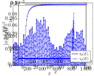
(b) $\lambda_{k}\approx 0.5$

Figure 1: The variation of the wavefunction of the wire along its length for (a) $\lambda_{k}\approx 0.03$ and (b) $\lambda_{k}\approx 0.5$. Other parameter values: $\mu=0$, $L=1000$.

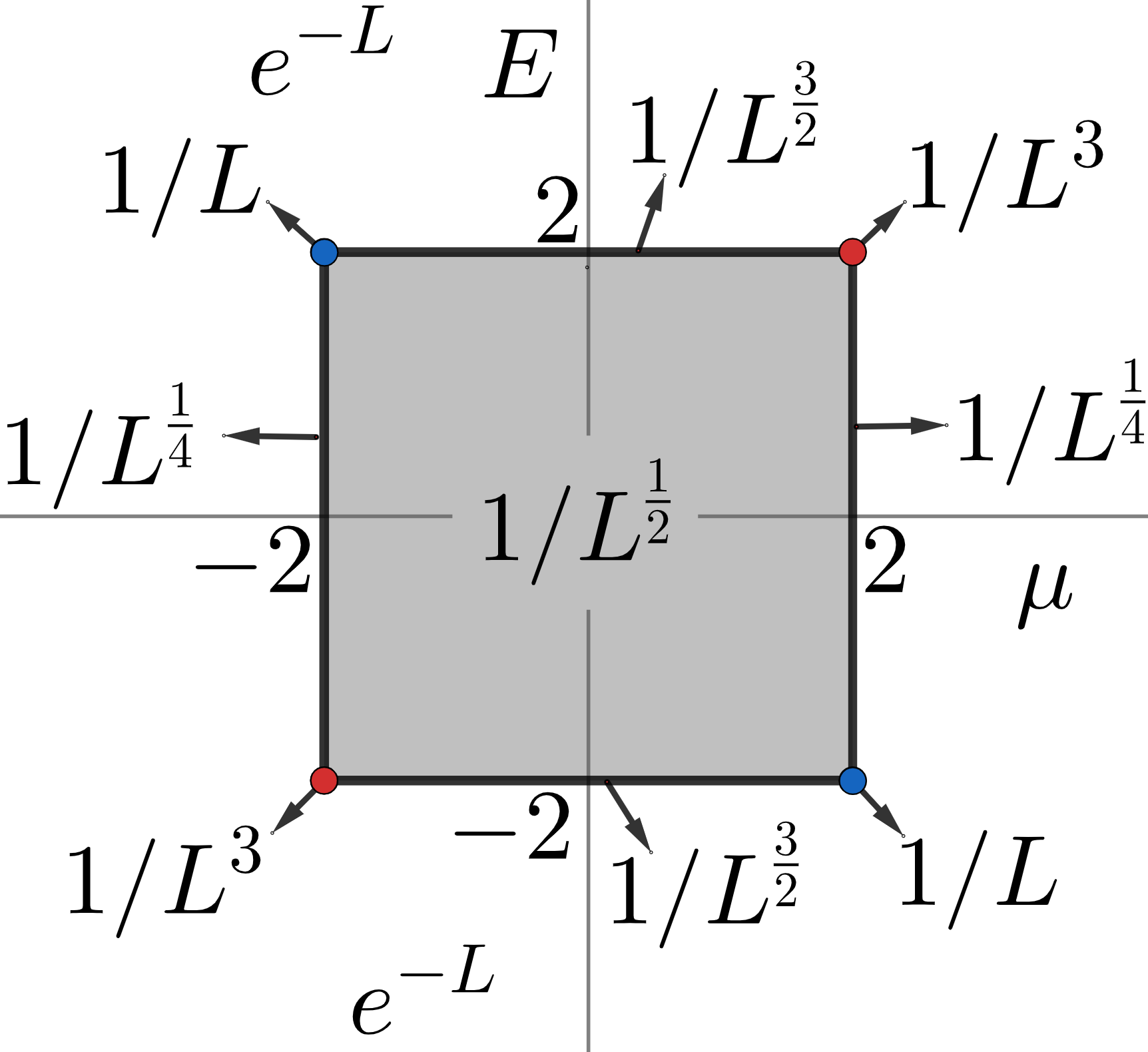
(a) $\expectationvalue{\epsilon}<0$

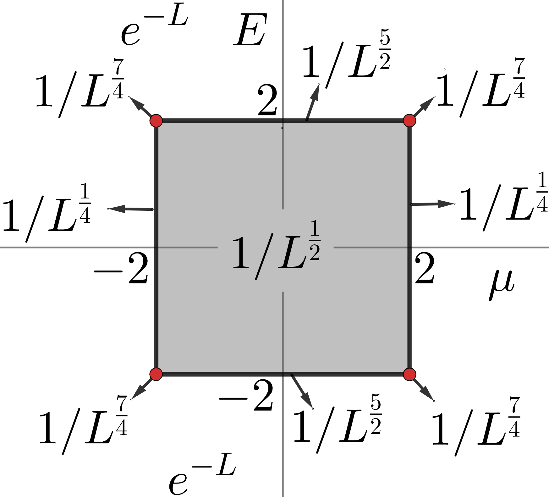
(b) $\expectationvalue{\epsilon}=0$

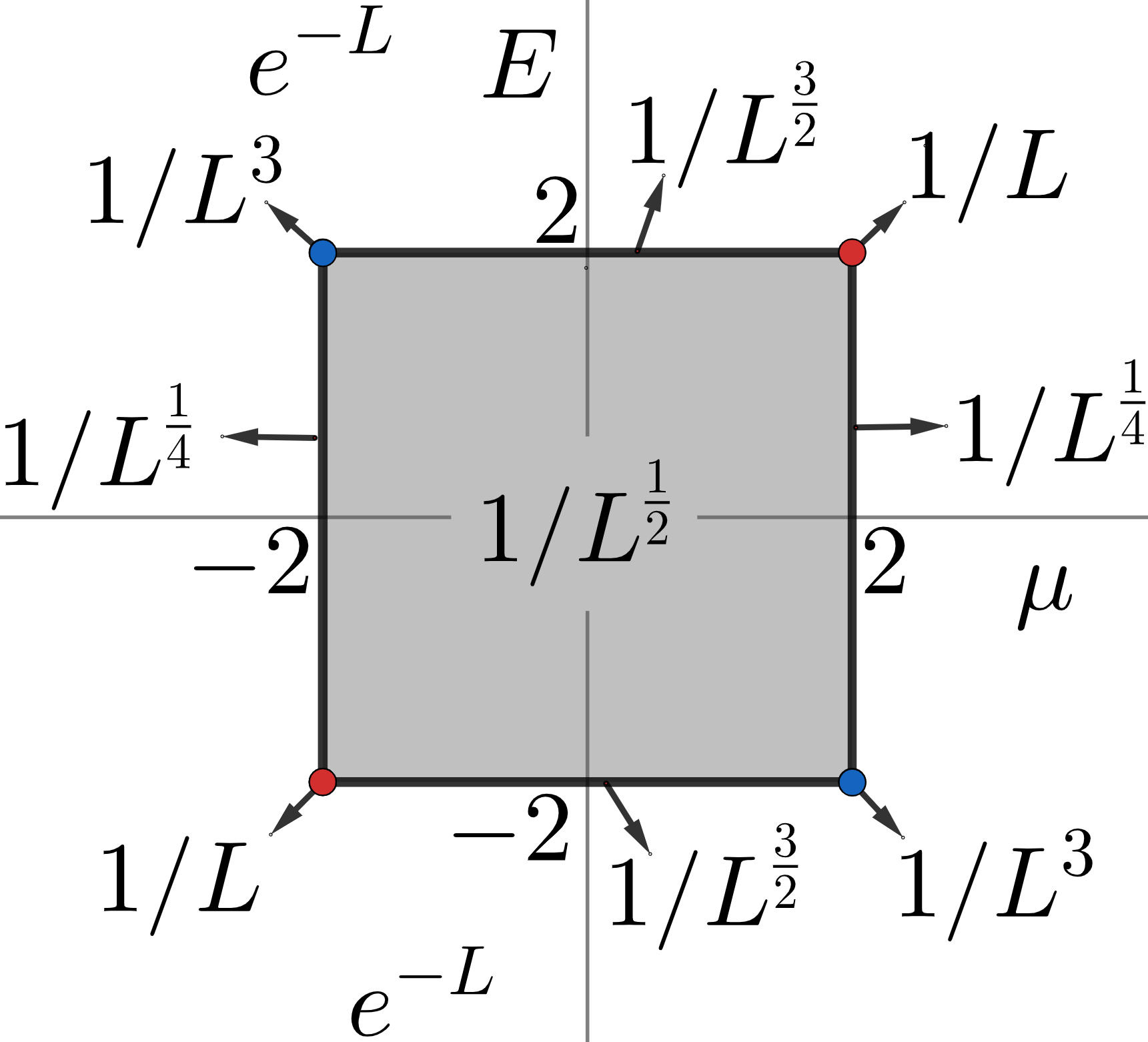
(c) $\expectationvalue{\epsilon}>0$

Figure 2: Power laws for the behavior of the conductance at different Fermi Levels and the parameter $\mu$.

III NEGF Conductance

The non-equilibrium steady state (NESS) of the wire can be obtained using the NEGF formalism. In this formalism, NESS is obtained starting from an initial state where the left and the right reservoirs described by grand canonical ensembles at temperatures $T_{L}$ and $T_{R}$ and chemical potentials $\mu_{L}$ and $\mu_{R}$, respectively, and the wire is chosen to be in an arbitrary state. It is then described in terms of the effective non-equilibrium Green’s function for the wire defined as Dhar and Sen (2006); Bhat and Dhar (2020),

$$G^{+}(E)=\frac{1}{E-H_{W}-\Sigma_{L}(E)-\Sigma_{R}(E)},$$ (10)

where $\Sigma_{L}(E)$ and $\Sigma_{R}(E)$ are the self energy contributions due to the reservoirs, and $H_{W}$ is the full hopping matrix of the wire. For $T_{L}=T_{R}=0$ and $\mu_{L}=E+\delta\mu$, $\mu_{R}=E-\delta\mu$, the conductance of the wire, in units of $e^{2}/h=1$, is given in terms of $G^{+}(E)$ as,

$$T(E)=4\pi^{2}\Tr[G^{+}(E)\Gamma_{R}(E)G^{-}(E)\Gamma_{L}(E)],$$ (11)

where $G^{-}(E)=[G^{+}(E)]^{\dagger}$ and $\Gamma_{L/R}=(\Sigma_{L/R}^{\dagger}-\Sigma_{L/R})/(2\pi i)$.

While the above formula holds for arbitrary lattice models, for our model this could be approximated by the following expression in the limit where $\eta_{bx}>>||E-H_{0}^{\prime}||,~{}(||.||~{}\text{denotes spectral norm of a matrix})$,

$$T(E)\approx 4\sum_{k=1}^{W}|F_{L}(\lambda_{k})|^{2},$$ (12)

where, $F_{L}(\lambda_{k})=\gamma^{2}/[p_{L}(\lambda_{k})+i\gamma[p_{L-1}(\lambda_{k})+q_{L}(\lambda_{k})]-\gamma^{2}q_{L-1}(\lambda_{k})]$ and $\gamma=\frac{\eta_{c}^{2}}{\eta_{bx}}$. For details see appendix A. Note that the $L$ dependence of the conductance comes completely from the functions $p_{L}(\lambda_{k})$, $q_{L}(\lambda_{k})$, respectively. These two obtained via same iteration equations,

$$p_{i+1}(\lambda_{k}) =(-E+\epsilon_{i+1}\lambda_{k})p_{i}(\lambda_{k})-p_{i-1}(\lambda_{k}),$$ (13)

$$q_{i+1}(\lambda_{k}) =(-E+\epsilon_{i+1}\lambda_{k})q_{i}(\lambda_{k})-q_{i-1}(\lambda_{k}),$$ (14)

but with the initial conditions,

$$p_{1}(\lambda_{k})=-E+\epsilon_{1}\lambda_{k},~{}~{}p_{0}(\lambda_{k})=1,~{}\text{and}$$ (15)

$$q_{1}(\lambda_{k})=1,~{}~{}q_{0}(\lambda_{k})=0,$$ (16)

respectively. Therefore, it suffices to consider only one of the two. The asymptotic behavior of the $p_{L}(\lambda_{k})$ with $L$ as $\lambda_{k}\rightarrow 0$ is what eventually controls the behavior of the conductance with $L$. Note that the iteration equation Eq. (13) is the same as Eq. (8), which gives the localization length of the eigenfunctions of the wire. We will discuss this iteration in the next section and look the behavior of $p_{L}(\lambda_{k})$ as $\lambda_{k}\rightarrow 0$. We end this section by taking the limit $W\rightarrow\infty$ for Eq. (12). The sum over $k$ in Eq. (12) sums over the eigenvalues of $H_{0}$ and in the limit $W\rightarrow\infty$, this sum can be replaced by an integral over the spectrum of $H_{0}$ given by $\mu+2\cos(\mathbf{k}),~{}\mathbf{k}\in(0,\pi)$,

$$\tau(E)=\frac{T(E)}{W}\approx\frac{4}{\pi}\int_{0}^{\pi}d\mathbf{k}|F_{L}(\lambda_{\mathbf{k}})|^{2},$$ (17)

where $\tau(E)$ is the conductance per unit width of the wire.

IV Analysis of the Lyapunov Exponents

Let us consider the iteration equation for $p_{L}(\lambda)$, we have

$$p_{i+1}(\lambda)=(-E+\epsilon_{i+1}\lambda)p_{i}(\lambda)-p_{i-1}(\lambda).$$ (18)

We have dropped the $k$ subscript on $\lambda$ for now and we will only consider $\lambda>0$ as $\lambda<0$ is equivalent to shifting the sign of the disorder parameter. We can rewrite the above equation in terms of products of independent and identically distributed random matrices of unit determinant as follows,

$$\begin{pmatrix}p_{L}(\lambda)\\ p_{L-1}(\lambda)\end{pmatrix}=\prod_{i=1}^{L}\begin{pmatrix}(-E+\epsilon_{i+1}\lambda)&&-1\\ 1&&0\end{pmatrix}\begin{pmatrix}p_{1}(\lambda)\\ p_{0}(\lambda)\end{pmatrix}.$$ (19)

$p_{L}(\lambda)$ grows exponentially as $L\rightarrow\infty$ for any non-zero $\lambda$ and for arbitrary initial conditions, even for a single realization of the disorder. This is due to the Furstenberg Theorem Furstenberg (1963) which guarantees non-negativity and the existence of the Lyapunov exponent defined as,

$$\zeta(\lambda)=\lim\limits_{L\rightarrow\infty}\frac{1}{L}\expectationvalue{\log|p_{L}(\lambda)|},$$ (20)

for any initial condition. The existence of the above limit implies that $\expectationvalue{p_{L}(\lambda)}\sim e^{L\zeta(\lambda)}$ as $L\rightarrow\infty$.

For $\lambda=0$, it is straightforward to see that $p_{L}(\lambda)$ does not grow exponentially for $|E|<2$, and therefore $\zeta(\lambda=0)=0$. So, as $\lambda\rightarrow 0$, $\zeta(\lambda)$ also approaches zero. Thus, $p_{L}(\lambda)$ does not grow exponentially with $L$ for $\lambda$ values such that $L\zeta(\lambda)<1$. Those values of $\lambda$ contribute in Eq. (17) for the conductance. The contribution from all other $\lambda$ values is exponentially small in $L$. To understand this more physically, we see that the localization length of the eigenvectors of the wire is given by the inverse of $\zeta(\lambda)$ and therefore the condition $L\zeta(\lambda)<1$ means that the localization length of the eigenvector which conducts is greater than the length of the wire. For $|E|>2$, $p_{L}(\lambda)$ grows exponentially even for $\lambda=0$, therefore the conductance scales as $e^{-L}$.

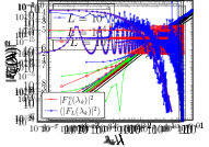
(d) $E=2,~{}\expectationvalue{\epsilon}<0$

Figure 3: Lyapunov exponents for the iteration equation, Eq. (18) for $|E|<2$ and $E=2$ with positive, negative and zero expectation value of the disorder. For $E=-2$, $\zeta(\lambda)\sim\lambda$ for $\expectationvalue{\epsilon}<0$ and $\zeta(\lambda)\sim\lambda^{1/2}$ for $\expectationvalue{\epsilon}>0$. The data presented is averaged over $10^{3}$ realizations of the disorder chosen uniformly from the intervals $(-1,0)$, $(-1,1)$ and $(0,1)$ for negative, zero and positive expectation value cases, respectively. .

The behavior of $\zeta(\lambda)$ near $\lambda=0$ is therefore crucial to the scaling of the conductance. We present numerical results on this behavior at different $E$ in Fig. (3). We see that while for $|E|<2$, $\zeta(\lambda)\sim\lambda^{2}$ irrespective of the expectation value of the disorder, for $|E|=2$ the behavior of $\zeta(\lambda)$ is different for positive, negative and zero expectation value of the disorder. For $E=2$, we find $\zeta(\lambda)\sim\lambda$, $\zeta(\lambda)\sim\lambda^{2/3}$, and $\zeta(\lambda)\sim\lambda^{1/2}$ for positive, zero and negative expectation value of the disorder, respectively. For $E=-2$, the behaviors are the same as $E=2$ except that $\zeta(\lambda)\sim\lambda^{1/2}$ for positive expectation value and $\zeta(\lambda)\sim\lambda$ for negative expectation value of the disorder.

We first consider the proof for the case of $|E|<2$ by following the steps of Matsuda and Ishii in Ref. Matsuda and Ishii, 1970. They considered the iteration equation, Eq. (18), for $E=-2$ and $\expectationvalue{\epsilon}<0$ in the context of classical harmonic wires with mass disorder. We only outline the proof for $|E|<2$ here leaving the details to appendix B. We start by making the change of variables,

$$\frac{p_{n+1}(\lambda)}{p_{n}(\lambda)}=\frac{\cos(\theta_{n}+h(\lambda,E))}{\cos\theta_{n}},$$ (21)

where $2\cos h(\lambda,E)=-E+\expectationvalue{\epsilon}\lambda$ so that the iteration equation now becomes,

$$\theta_{n+1}=\arctan\left[\tan(\theta_{n}+h(\lambda,E))+\frac{\lambda(\epsilon-\expectationvalue{\epsilon})}{\sin h(\lambda,E)}\right]=\bar{\Theta}[\theta_{n},\lambda].$$ (22)

The Lyapunov exponent in terms of the variable $\theta$, is given by

$$\zeta(\lambda) =\lim\limits_{L\rightarrow\infty}\frac{1}{L}\expectationvalue{\sum_{n=1}^{L}\log\absolutevalue{\frac{\cos(\theta_{n}+h(\lambda,E))}{\cos\theta_{n}}}},$$ (23)

$$=\int_{-\pi/2}^{\pi/2}d\theta~{}\mathbf{P}[\theta,\lambda]\log\absolutevalue{\frac{\cos(\theta+h(\lambda,E))}{\cos\theta}}.$$ (24)

In the last step we have replaced the average over ”time” in the Marko process defined by the iteration equation, Eq. (18), by the integral over the invariant distribution $\mathbf{P}[\theta,\lambda]$ of the Marko process in accordance with the ergodic hypothesis. Expanding Eq. (24) in orders of $\lambda$ we have,

$$\zeta(\lambda)=\int_{-\pi/2}^{\pi/2} d\theta\log|\cos\theta|\bigg{[}\boldsymbol{\zeta}_{0}(\theta,E)+\lambda\boldsymbol{\zeta}_{1}(\theta,E)$$

$$+\lambda^{2}\boldsymbol{\zeta}_{2}(\theta,E)+\order{\lambda^{3}}\bigg{]}.$$ (25)

Assuming $h(\lambda,E)=\sum_{i=0}^{\infty}h_{i}(E)\lambda^{i}$ and $\mathbf{P}[\theta,\lambda]=\sum_{i=0}^{\infty}\mathbf{P}_{i}(\theta)\lambda^{i}$, the coefficients $\boldsymbol{\zeta}_{i}(\theta,E)$ depend on $\theta$ and $E$ via the functions $\mathbf{P}_{i}(\theta)$ and $h_{i}(E)$. Therefore, we need to determine $\mathbf{P}[\theta,\lambda]$ at least up to order $\lambda^{2}$ to find $\zeta(\lambda)$. It can be shown that the invariant distribution satisfies the self-consistent equation,

$$\mathbf{P}[\theta,\lambda]-\int d\epsilon~{}\mathbf{P}[\Theta[\theta,\lambda],\lambda]\partial_{\theta}\Theta[\theta,\lambda]\mathbf{p}(\epsilon)=0,$$ (26)

where $\mathbf{p}(\epsilon_{x})$ is the probability distribution for $\epsilon_{x}$ and

$$\Theta[\theta,\lambda]=\arctan\left[\tan\theta-\frac{\lambda(\epsilon-\expectationvalue{\epsilon})}{\sin h(\lambda,E)}\right]-h(\lambda,E),$$ (27)

is the inverse of the function $\bar{\Theta}[\theta,\lambda]$. Expanding the L.H.S of Eq. 26 in orders of $\lambda$ and setting each order to zero gives, $\boldsymbol{\zeta}_{0}(\theta,E)=0$, $\boldsymbol{\zeta}_{1}(\theta,E)=0$, and $\boldsymbol{\zeta}_{2}(\theta,E)\neq 0$ for the zeroth, first and second order in $\lambda$, respectively. Hence, the zeroth order and the first order terms vanish in the expansion of $\zeta(\lambda)$ and therefore $\zeta(\lambda)\sim\lambda^{2}$ as $\lambda\rightarrow 0$.

The proof relies on the fact that $\theta\in(-\pi/2,\pi/2)$ is bounded which is true as long as $h(\lambda,E)$ is real or equivalently $|-E+\expectationvalue{\epsilon}\lambda|<2$. Therefore, it also works for the cases where $E=-2$, $\expectationvalue{\epsilon}<0$ and $E=2$, $\expectationvalue{\epsilon}>0$. However, when $|E|=2$, the expansion for $h(\lambda,E)$ is different as it has half integer powers of $\lambda$. This makes the leading contribution to the Lyapunov exponent, $\zeta(\lambda)\sim\lambda$ for the two cases.

For $|-E+\expectationvalue{\epsilon}\lambda|\geq 2$, the above proof does not hold. The cases where this happens are $|E|=2$ with $\expectationvalue{\epsilon}=0$, $E=2$ with $\expectationvalue{\epsilon}<0$, and $E=-2$ with $\expectationvalue{\epsilon}<0$. Let us first consider the latter two cases. For these cases the Lyapunov exponent is finite even if the disorder is replaced by its average, $\expectationvalue{\epsilon}$. In that case, the solution for Eq. (18) is given by $p_{L}(\lambda)=\frac{\sin(L+1)h(\lambda)}{\sin h(\lambda)}.$ Therefore, in the limit $L\rightarrow\infty$, $p_{L}(\lambda)\sim e^{\sqrt{\expectationvalue{\epsilon}\lambda}L}$ which gives $\zeta(\lambda)\sim\lambda^{1/2}$. The disorder only contributes at higher orders in $\lambda$. The case where $\expectationvalue{\epsilon}=0$ is very subtle and requires an elaborate proof. We point the reader to Ref. (Cane et al., 2021) which considers Eq. (18) for $E=-2$ in the context of harmonic wires with disordered magnetic fields. In this work, the Lyapunov exponents are determined by mapping Eq. (18) for $E=-2$ to a harmonic oscillator with noisy frequency Crauel et al. (1999). It is shown that $\zeta(\lambda)\sim\lambda^{2/3}$ for $\expectationvalue{\epsilon}=0$, and also $\zeta(\lambda)\sim\lambda^{1/2}$ and $\zeta(\lambda)\sim\lambda$ for $\expectationvalue{\epsilon}>0$ and $\expectationvalue{\epsilon}<0$, respectively.

Having discussed the Lyapunov exponents, we now proceed to the next section where we use these results to determine the average behavior of the conductance with the system size.

(a)  $|E|<2$

(b) $E=2,~{}\expectationvalue{\epsilon}>0$

(c) $E=2,~{}\expectationvalue{\epsilon}=0$

V Scaling of the Conductance

In this section, we determine the scaling of the average behavior of the conductance. Let us assume $\zeta(\lambda_{\mathbf{k}})\sim|\lambda_{\mathbf{k}}|^{a}$, where $a$ is determined by the results of Sec. (IV). Therefore, the $|\lambda_{\mathbf{k}}|$ values for which $|\lambda_{\mathbf{k}}|^{a}L<1$ contribute in the integral for the conductance in Eq. (17). Hence, in the limit $L\rightarrow\infty$, we can cutoff the integral over $\mathbf{k}$ around the point where $\lambda_{\mathbf{k}}$ vanishes as follows,

$$\expectationvalue{\tau(E)}\approx\frac{4}{\pi}\lim\limits_{L\rightarrow\infty}\int_{\mathbf{k}_{*}-\mathbf{k}_{c}}^{\mathbf{k}_{*}+\mathbf{k}_{c}}d\mathbf{k}\expectationvalue{|F_{L}(\lambda_{\mathbf{k}})|^{2}},$$ (28)

where $\mathbf{k}_{*}$ is the point where $\lambda_{\mathbf{k}=\mathbf{k}_{*}}=0$, and $\mathbf{k}_{c}>0$ is a small deviation from $\mathbf{k}_{*}$ such that $|\lambda_{\mathbf{k}_{*}+\mathbf{k}_{c}}|^{a}L\sim 1$. Let the Taylor expansion of $\lambda_{\mathbf{k}}$ around $\mathbf{k}=\mathbf{k}_{*}$ be $\lambda_{\mathbf{k}_{*}+\mathbf{k}_{c}}=\lambda_{0}\mathbf{k}_{c}^{b}+\order{\mathbf{k}_{c}^{b+1}}$, we have $\mathbf{k}_{c}\sim 1/L^{1/(ab)}$. We see that the “number” of $\lambda$ contributing to the transport itself scales with $L$ as $1/L^{ab}$, and each of these $\lambda$ corresponds to an eigenvector of the wire with eigenvalue lying near $E$. This makes the scaling of conductance with the length of the wire effectively a power-law. To determine this power-law, the integrand in Eq. (28) needs a bit more attention.

Within the range of integration in Eq. (28), the disorder is effectively absent so we make an assumption by replacing $\expectationvalue{F_{L}(\lambda_{\mathbf{k}})}$ by $F_{L}^{o}(\lambda_{\mathbf{k}})$ which is the same quantity computed with the disorder replaced by its average at every $x$. With some simple algebra we can show,

$$F_{L}^{o}(\lambda_{\mathbf{k}})=\frac{\gamma\sin q_{\mathbf{k}}}{\sin q_{\mathbf{k}}(L+1)+2i\gamma\sin q_{\mathbf{k}}L-\gamma^{2}\sin q_{\mathbf{k}}(L-1)}$$ (29)

where $q_{\mathbf{k}}=\arccos\frac{-E+\expectationvalue{\epsilon}\lambda_{\mathbf{k}}}{2}$. To justify this assumption, we show in Fig. (4) a plot comparing $F_{L}^{o}(\lambda_{\mathbf{k}})$ with $\expectationvalue{F_{L}^{o}(\lambda_{\mathbf{k}})}$ at different $\lambda_{\mathbf{k}}$. We see a good match as $\lambda_{\mathbf{k}}\rightarrow 0$. Using this assumption Eq. (28) reduces to,

$$\expectationvalue{\tau(E)}\approx\frac{4}{\pi}\lim\limits_{L\rightarrow\infty}\int_{\mathbf{k}_{*}-\mathbf{k}_{c}}^{\mathbf{k}_{*}+\mathbf{k}_{c}}d\mathbf{k}|F_{L}^{o}(\lambda_{\mathbf{k}})|^{2}.$$ (30)

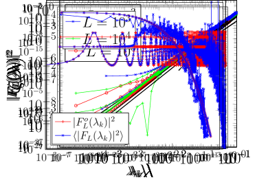
Figure 4: Comparison between $\expectationvalue{F_{L}(\lambda_{\mathbf{k}})}$ and $F_{L}^{o}(\lambda_{\mathbf{k}})$ for $E=0$ and $\mu=0$ with the size of the wire as $L=10^{3},~{}W=10^{4}$. We see that the two quantities show a good agreement as $\lambda_{\mathbf{k}}\rightarrow 0$. The data presented for $\expectationvalue{F_{L}(\lambda_{\mathbf{k}})}$ is averaged over $10^{3}$ realizations of the disorder chosen uniformly from the interval $(0,1)$, respectively. Other parameter values: $\gamma=0.25$.

The scaling of the conductance depends on how $F_{L}^{o}(\lambda_{\mathbf{k}})$ behaves around $\mathbf{k}=\mathbf{k}_{*}$ in the limit $L\rightarrow\infty$. From Eq. (29), if $q_{\mathbf{k}}$ is real then $F_{L}^{o}(\lambda_{\mathbf{k}})$ is highly oscillatory with $L$. However, under the integral sign it averages out to a smooth curve. It can be shown that in the limit $L\rightarrow\infty$, oscillations in $F_{L}^{o}(\lambda_{\mathbf{k}})$ averages out to $\bar{F}^{o}(q_{\mathbf{k}})$ given by,

$$\bar{F}^{o}(q_{\mathbf{k}})=\frac{\gamma}{2(1+\gamma^{2})}\sin q_{\mathbf{k}},$$ (31)

under the integral sign. For the derivation of this result see appendix C. Using this in Eq. (30) we have,

$$\expectationvalue{\tau(E)}\approx\frac{1}{\pi}\frac{2\gamma}{1+\gamma^{2}}\int_{\mathbf{k}_{*}-\mathbf{k}_{c}}^{\mathbf{k}_{*}+\mathbf{k}_{c}}d\mathbf{k}\sin q_{\mathbf{k}}$$ (32)

Substituting $\mathbf{k}_{c}$ to be $1/L^{ab}$, shifting the integral by $\mathbf{k}_{*}$ and dropping the factors independent of $L$ we have,

$$\expectationvalue{\tau(E)}\sim\int_{-1/L^{1/(ab)}}^{L^{1/(ab)}}d\mathbf{\bar{k}}\sin q_{\mathbf{\bar{k}}+\mathbf{k}_{*}}.$$ (33)

Note that going from Eq. (30) to Eq. (33) is valid only if $F_{L}^{o}(\lambda_{\mathbf{k}})$ behaves oscillatory around $\mathbf{k}=\mathbf{k}_{*}$, i.e. $\absolutevalue{-E+\lambda_{0}\expectationvalue{\epsilon}\mathbf{\bar{k}}^{b}}<2$ within the range of the integration. The term $\lambda_{0}\expectationvalue{\epsilon}\mathbf{\bar{k}}^{b}$ is of the order of $1/L^{1/{a}}$ and becomes important only when $|E|=2$ where the sign of $\lambda_{0}\expectationvalue{\epsilon}\mathbf{\bar{k}}^{b}$ also becomes important. We therefore have the following cases:

• $|E|<2$, $|\mu|<2$: In this case, $a=2$ and $b=1$ which gives $\mathbf{k}_{c}\sim 1/L^{1/2}$. Also, the integrand, $\sin q_{\mathbf{\bar{k}}+\mathbf{k}_{*}}$, in Eq. (33) is finite at $\mathbf{\bar{k}}=0$, therefore we have,

  $$\expectationvalue{\tau(E)}\sim\int_{-1/L^{1/2}}^{L^{1/2}}d\mathbf{\bar{k}}\sim\frac{1}{L^{1/2}},$$ (34)

  where we have dropped the pre-factors that do not depend on $L$.

• $|E|<2$, $|\mu|=2$: This case is the same as A1 except the behavior of $\lambda_{\mathbf{k}}$ around $\mathbf{k}=\mathbf{k}_{*}$ changes and therefore $b=2$ giving,

  $$\expectationvalue{\tau(E)}\sim\frac{1}{L^{1/4}}.$$ (35)

• $|E|=2$, $|\mu|<2$ and $\expectationvalue{\epsilon}\neq 0$: We discuss for $E=2$ as similar arguments can given for $E=-2$. As $|\mu|<2$, $b=1$ and therefore, $\absolutevalue{-E+\lambda_{0}\expectationvalue{\epsilon}\mathbf{\bar{k}}}<2$ only for $\expectationvalue{\epsilon}\mathbf{\bar{k}}\lambda_{0}>0$. Now for this case $\lambda_{0}<0$, therefore, $\expectationvalue{\epsilon}\mathbf{\bar{k}}\lambda_{0}>0$ only for $\expectationvalue{\epsilon}>0,\mathbf{\bar{k}}>0$ or $\expectationvalue{\epsilon}<0,\mathbf{\bar{k}}<0$. Therefore, for say $\expectationvalue{\epsilon}>0$, the Lyapunov exponents are given by $\lambda_{\mathbf{k}}$ and $\lambda_{\mathbf{k}}^{1/2}$, for $\mathbf{\bar{k}}>0$ and $\mathbf{\bar{k}}<0$, respectively because change in the sign of $\mathbf{\bar{k}}$ is effectively changing the sign of the disorder. This means that different contributions come from the positive and negative half of the integral in Eq. (33) as the cutoff limits of the integration are different. For the positive half $\mathbf{k}_{c}\sim 1/L$ and for the negative half , $\mathbf{k}_{c}\sim 1/L^{2}$. Therefore, we have

  $$\expectationvalue{\tau(E)} \sim\int_{0}^{1/L}d\mathbf{\bar{k}}\sin q_{\mathbf{\bar{k}}+\mathbf{k}_{*}}+\lim\limits_{L\rightarrow\infty}\int^{0}_{-1/L^{2}}d\mathbf{\bar{k}}|F_{L}^{o}(\lambda_{\mathbf{k}})|^{2}$$ (36)

  $$\sim\int_{0}^{1/L}d\mathbf{\bar{k}}~{}\mathbf{\bar{k}}^{1/2}\sim\frac{1}{L^{3/2}},$$ (37)

  where we have ignored the contribution from the negative part as it is subdominant. Similar arguments giving the same power-law can be made for $\expectationvalue{\epsilon}<0$. Note a key difference of this case from previous two cases, $\sin q_{\mathbf{k}_{*}}$ vanishes as $|E|=2$, so the leading term of the integrand is given by $\mathbf{\bar{k}}^{1/2}$, contributing to the power-law.

• $E=\mu=2$ or $E=\mu=-2$ and $\expectationvalue{\epsilon}>0$: We only discuss $E=\mu=2$, as similar arguments can be made for $E=\mu=-2$. For $\mu=2$, $\mathbf{k}_{*}=\pi$ therefore $b=2$ and $\lambda_{0}>0$. Hence, $|-E+\lambda_{0}\expectationvalue{\epsilon}\mathbf{\bar{k}}^{2}|<2$ only when $\expectationvalue{\epsilon}>0$. Also, $a=1$, and therefore,

  $$\expectationvalue{\tau(E)} \sim\int_{-1/L^{1/2}}^{1/L^{1/2}}d\mathbf{\bar{k}}\sin q_{\mathbf{\bar{k}}+\mathbf{k}_{*}}$$ (38)

  $$\sim\int_{-1/L^{1/2}}^{1/L^{1/2}}d\mathbf{\bar{k}}|\mathbf{\bar{k}}|~{}\sim\frac{1}{L},$$ (39)

• $E=-\mu=2$ or $-E=\mu=2$ and $\expectationvalue{\epsilon}<0$: Similar arguments as for A4 give $\expectationvalue{\tau(E)}\sim 1/L$ for this case also.

(a)  A1

(b)  A2

(c)  A3

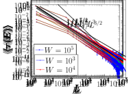
(d)  A4

Figure 5: Numerically observed power-laws for the cases A1-A4. We see a good agreement with the predicted values as the width of the wire is increased. The data presented is averaged over $10^{3}$ disorder realizations. Parameter values for A1 are $E=\mu=0$, for A2 $E=0,~{}\mu=2$, for A3 $\mu=0~{},E=2$ and for A4 $E=\mu=2$, $\gamma=0.25$.

A numerical computation of the conductance for these cases is shown in Fig. (5) and a very good agreement is seen between theoretically expected values and the numerically observed powerlaws.

(a)  B1

(b)   B1

(c)   B2

(d)   B2

(e)   B3

(f)   B3

Figure 6: Numerically observed power-laws for the cases B1-B3. We see that for B1 and B2 the numerically computed power laws are larger by a factor of $L$ compared to the theory. This is due to underestimation of $\expectationvalue{F_{L}(\lambda_{\mathbf{k}})}$ by the theory as can be seen in the corresponding adjacent plots for $W=10^{4}$ and $L=10^{3}$. The blue curve lies above the red curve which is the estimation from the theory. For the case B3, a good agreement is seen with the theory. The disorder is chosen uniformly from the interval $(-1,1)$ and $(-1,0)$ for B1/B2 and B3, respectively and the data presented is averaged over $10^{3}$ realizations. Other parameter values: for B1 $E=2$, $\mu=0$, for B2 $E=\mu=2$ and from B3 $E=\mu=2$, $\gamma=0.25$.

Let us now consider the cases where, $F_{L}^{o}(\lambda_{\mathbf{k}})$ is no longer oscillatory, this happens when $|-E+\expectationvalue{\epsilon}\lambda_{\mathbf{k}}|\geq 2$. The different cases are the following,

• $|E|=2$, $\mu<2$ and $\expectationvalue{\epsilon}$=0: In this case, $q_{\mathbf{k}_{*}}=\pi$ and therefore, $\lim\limits_{q_{\mathbf{k}_{*}}\rightarrow\pi}F_{L}^{o}(\lambda_{\mathbf{k}})=\gamma/(L+1+2i\gamma L-\gamma^{2}(L-1))$. In the limit, $L\rightarrow\infty$, $F_{L}^{o}(\lambda_{\mathbf{k}})\sim 1/L$. Using this in the integral of Eq. (30) and that $a=2/3$, $b=1$, we have

  $$\expectationvalue{\tau(E)}\sim\frac{1}{L^{2}}\int_{\mathbf{k}_{*}-L^{3/2}}^{\mathbf{k}_{*}+L^{3/2}}d\mathbf{k}\sim\frac{1}{L^{7/2}}.$$ (40)

• $|E|=|\mu|=2$ and $\expectationvalue{\epsilon}$=0: Using the same arguments as in the case B1, $F_{L}^{o}(\lambda_{\mathbf{k}})\sim L$, in the limit $L\rightarrow\infty$. Using this and that $b=2$ and $a=2/3$ in the integral of Eq. (30), we have

  $$\expectationvalue{\tau(E)}\sim\frac{1}{L^{2}}\int_{\mathbf{k}_{*}-L^{3/4}}^{\mathbf{k}_{*}+L^{3/4}}d\mathbf{k}\sim\frac{1}{L^{11/4}}$$ (41)

• $E=\mu=2$ or $E=\mu=-2$ and $\expectationvalue{\epsilon}<0$: For this case $\mathbf{k}_{c}\sim 1/L$ and a Taylor expansion of $F_{L}^{o}(\lambda_{\mathbf{k}})$ around $\mathbf{k}_{*}$ with $|\mathbf{k}_{*}-\mathbf{k}|<<1/L$ once again gives $F_{L}^{o}(\lambda_{\mathbf{k}})\sim 1/L$ as $L\rightarrow\infty$. This gives the power-law to be,

  $$\expectationvalue{\tau(E)}\sim\frac{1}{L^{2}}\int_{\mathbf{k}_{*}-(1/L)}^{\mathbf{k}_{*}+1/L}d\mathbf{k}\sim\frac{1}{L^{3}}.$$ (42)

• $-E=\mu=2$ or $E=-\mu=2$ and $\expectationvalue{\epsilon}>0$: This case is the same as B3.

Fig. (6) shows a comparison with the numerically calculated conductance for the above three cases. We see that the theoretical arguments underestimate the power-law approximately by a factor of $L$ for the above the cases where $\expectationvalue{\epsilon}=0$ i.e. B1 and B2. While the theory predicts $1/L^{7/2}$ and $1/L^{11/4}$ for the two cases, numerical data agrees with $1/L^{5/2}$ and $1/L^{7/4}$, respectively. The reason being that the approximation that $|F_{L}^{o}(\lambda_{\mathbf{k}})|=\expectationvalue{|F_{L}(\lambda_{\mathbf{k}})|}$ for $\lambda_{\mathbf{k}}\rightarrow 0$ fails and in fact it underestimates $\expectationvalue{|F_{L}(\lambda_{\mathbf{k}})|}$ as can be seen that the blue curve lies above the red curve in Fig. (6b) and Fig. (6d), respectively. The red curve is constant as for $\expectationvalue{\epsilon}=0$ the dependence on $\lambda_{\mathbf{k}}$ vanishes for $F_{L}^{o}(\lambda_{\mathbf{k}})$. It is not clear how to estimate $\expectationvalue{F_{L}(\lambda_{\mathbf{k}})}$ and predict the observed power-laws for these two cases, and therefore our work opens up an interesting question for further studies. A similar issue has also been pointed out for harmonic wires in presence of disordered magnetic fields . For the case B3, we see a perfect agreement between the theory and the numerical computations.

VI Conclusions

In conclusion, we looked at a model of a disordered Fermionic wire in two-dimensions and studied the scaling of conductance with the length of the wire along the direction of transport. In particular, we find that despite the disorder the conductance shows a super-diffusive scaling due to presence of eigenstates with diverging localization lengths within energies with absolute values less than some cutoff $E_{c}$. These eigenstates correspond to $\lambda_{\mathbf{k}}\rightarrow 0$, where $\lambda_{\mathbf{k}}$ are eigenvalues of the matrix $H_{0}$ defined in Eq. (2). Using heuristic arguments, we determined the super-diffusive behavior to be $1/L^{1/2}$ which agrees with the numerical computations. We also showed that at $E=E_{c}$ and at some special values of the parameters of the wire the conductance shows various sub-diffusive behaviors summarized in Fig. (2). The sub-diffusive power-laws are sensitive to the the sign of the expectation value of the disorder and are also different if the expectation value of the disorder vanishes.

Our theoretical arguments predict the sub-diffusive power-laws in all the cases except for the case where the disorder average vanishes. For this case, the key approximation that as $\lambda_{\mathbf{k}}\rightarrow 0$, the disorder parameter at each site can be replaced by its average breaks down and underestimates the numerically observed power-law by a factor of $L$. This case therefore requires further study in order to correctly predict the numerically observed power-laws.

VII Acknowledgments

I thank Marko Žnidarič and Yu-Peng Wang for useful discussions. I also acknowledge support by Grant No. J1-4385 from the Slovenian Research Agency.

Appendix A Simplification of NEGF Conductance

Since the contacts with the reservoirs are only along the edges i.e. at $x=1$, and $x=L$, the trace in Eq. (11) can be computed as,

$$T(E)=4\pi^{2}\Tr[\tilde{G}^{+}_{1L}\tilde{\Gamma}\tilde{G}^{-}_{L1}\tilde{\Gamma}],$$ (43)

where $\tilde{G}^{+}_{1L}=[P_{L}+\tilde{\Sigma}P_{L-1}+Q_{L-1}\tilde{\Sigma}+\tilde{\Sigma}Q_{L-2}\tilde{\Sigma}]^{-1}$ Bhat (2024). The tilde over the Green function and self energy matrices denotes that these are written in the diagonal basis of $H_{0}$ i.e. $\tilde{G}^{+}_{1L}[y,y^{\prime}]=-UG^{+}(E)[x=1,y;x^{\prime}=L,y^{\prime}]U^{\dagger}$ where $G^{+}(E)[x=1,y;x^{\prime}=L,y^{\prime}]$ is the $(1,L)$ block of the full Green’s function matrix, $G^{+}(E)$ and $U$ diagonalizes $H_{0}$. Similarly, $\tilde{\Sigma}[y,y^{\prime}]=U\Sigma[y,y^{\prime}]U^{\dagger}=U\Sigma_{R}[L,y;L,y^{\prime}]U^{\dagger}=U\Sigma_{L}[1,y;1,y^{\prime}]U^{\dagger}$, $\tilde{\Gamma}[y,y^{\prime}]=U\Gamma[y,y^{\prime}]U^{\dagger}=U\Gamma_{R}[L,y;L,y^{\prime}]U^{\dagger}=U\Gamma_{L}[1,y;1,y^{\prime}]U^{\dagger}$ are the only non-zero blocks of the matrices $\Sigma_{L/R}$ and $\Gamma_{L/R}$. It can be shown that $\Sigma=U_{L}\Sigma_{D}U_{L}^{\dagger}$, where $\Sigma_{D}$ is a diagonal matrix with components given by Dhar and Sen (2006),

$$\Sigma_{D}[k,k]=\begin{cases}\frac{\eta_{c}^{2}}{\eta_{bx}}[z_{k}+i\sqrt{1-z_{k}^{2}}];&|z_{k}|<1,\\ \frac{\eta_{c}^{2}}{\eta_{bx}}[z_{k}-\sqrt{z_{k}^{2}-1}];&z_{k}>1,\\ \frac{\eta_{c}^{2}}{\eta_{bx}}[z_{k}+\sqrt{z_{k}^{2}-1}];&z_{k}<-1,\end{cases}$$ (44)

where $z_{k}=\frac{\omega-\tilde{\lambda}_{k}}{2\eta_{bx}}$. $U_{L}$ is the unitary transformation that diagonalizes the intra-chain hopping matrix $\tilde{H}_{0}$ of the reservoirs and its eigenvalues are given by $\tilde{\lambda}_{k}$, $k=1,2,...,W$. We consider the limit where $|\eta_{bx}|>>|\omega-\tilde{\lambda}_{k}|$ for all $k$. In that case, $\tilde{\Sigma}\approx\Sigma\approx\Sigma_{D}\approx i\gamma I$ and $\Gamma\approx\frac{\gamma}{\pi}I$, where $\gamma=\eta_{c}^{2}/\eta_{bx}$. Thus, Eq. (43) reduces to,

$$T(E)\approx$$

$$4\sum_{k=1}^{W}\frac{\gamma^{2}}{|p_{L}(\lambda_{k})+i\gamma[p_{L-1}(\lambda_{k})+q_{L}(\lambda_{k})]-\gamma^{2}q_{L-1}(\lambda_{k})|^{2}}$$ (45)

$$=4\sum_{k=1}^{W}|F_{L}(\lambda_{k})|^{2}$$ (46)

which is the same as Eq. (12).

Appendix B Lyapunov Exponent Proof

We begin rewriting Eq. (24) as,

$$\zeta(\lambda) =\int_{-\pi/2}^{\pi/2}d\theta~{}\mathbf{P}[\theta,\lambda]\log\absolutevalue{\frac{\cos(\theta+h(\lambda,E))}{\cos\theta}}$$ (47)

$$=\int_{-\pi/2}^{\pi/2}d\theta~{}(\mathbf{P}[\theta-h(\lambda),\lambda]-\mathbf{P}[\theta,\lambda])\log|\cos\theta|$$ (48)

We have used the fact that $\mathbf{P}[\theta,\lambda]$ is periodic as the iteration equation, Eq. 22, is itself periodic in the variable $\theta$. We Taylor expand Eq. (48) around $\lambda=0$, to obtain the coefficients $\boldsymbol{\zeta}_{0}(\theta,E)$, $\boldsymbol{\zeta}_{1}(\theta,E)$ and $\boldsymbol{\zeta}_{2}(\theta,E)$ as,

$$\boldsymbol{\zeta}_{0}(\theta,E) =\big{[}\mathbf{P}_{0}(\theta-h_{0}(E))-\mathbf{P}_{0}(\theta)\big{]}$$ (49)

$$\boldsymbol{\zeta}_{1}(\theta,E) =-h_{1}(E)\partial_{\theta}\mathbf{P}_{0}(\theta-h_{0}(E))$$

$$~{}~{}~{}~{}~{}+\mathbf{P}_{1}(\theta-h_{0}(E))-\mathbf{P}_{1}(\theta)$$ (50)

$$\boldsymbol{\zeta}_{2}(\theta,E) =-h_{2}(E)\partial_{\theta}\mathbf{P}_{0}(\theta-h_{0}(E))+\frac{h_{1}(E)^{2}}{2}\partial_{\theta}^{2}\mathbf{P}_{0}(\theta-h_{0}(E))$$

$$-h_{1}(E)\partial_{\theta}\mathbf{P}_{1}(\theta-h_{0}(E))+\mathbf{P}_{2}(\theta-h_{0}(E))-\mathbf{P}_{2}(\theta).$$ (51)

Let us now Taylor expand the self consistency equation of $\mathbf{P}[\theta,\lambda]$ Eq. (26). We have,

$$\mathbf{P}_{0}(\theta)-\mathbf{P}_{0}(\theta-h_{0}(E))=0,$$ (52)

$$\mathbf{P}_{1}(\theta)-\bigg{[}\partial_{\theta}\mathbf{P}_{0}(\theta-h_{0}(E))\expectationvalue{\Theta_{1}}+\mathbf{P}_{1}(\theta-h_{0}(E))+\partial_{\theta}\expectationvalue{\Theta_{1}}\mathbf{P}_{0}(\theta-h_{0}(E))\bigg{]}=0,$$ (53)

$$\mathbf{P}_{2}(\theta)-\bigg{[}\mathbf{P}_{2}(\theta-h_{0}(E))+\partial_{\theta}\mathbf{P}_{0}(\theta-h_{0}(E))\expectationvalue{\Theta_{2}}+\frac{1}{2}\partial_{\theta}^{2}\mathbf{P}_{0}(\theta-h_{0}(E))\expectationvalue{\Theta_{1}^{2}}+\partial_{\theta}\mathbf{P}_{1}(\theta-h_{0}(E))\expectationvalue{\Theta_{1}}$$

$$+\mathbf{P}_{0}(\theta-h_{0}(E))\partial_{\theta}\expectationvalue{\Theta_{2}}+(\partial_{\theta}\mathbf{P}_{0}(\theta-h_{0}(E))\expectationvalue{\Theta_{1}}+\mathbf{P}_{1})(\partial_{\theta}\expectationvalue{\Theta_{1}})\bigg{]}=0,$$ (54)

where we assumed $\Theta[\theta,\lambda]=\theta-h_{0}(E)+\sum_{i=1}^{\infty}\Theta_{i}(\theta)\lambda^{i}$. Eq. (52) immediately gives $\boldsymbol{\zeta}_{0}(\theta,E)=0$. To show that $\boldsymbol{\zeta}_{1}(\theta,E)=0$, we consider the expansion of functions $\expectationvalue{\Theta[\theta,\lambda]}$ and $h(\lambda,E)$ around $\lambda=0$,

$$h(\lambda) =h_{0}(E)-\frac{\expectationvalue{\epsilon}\lambda}{(4-E^{2})^{1/2}}+\frac{E\expectationvalue{\epsilon}^{2}\lambda^{2}}{2(4-E^{2})^{3/2}}+\order{\lambda^{3}}$$ (55)

$$\expectationvalue{\Theta[\theta,\lambda]} =\theta-h_{0}(E)+\frac{\expectationvalue{\epsilon}\lambda}{(4-E^{2})^{1/2}}$$

$$-\left[\frac{E\expectationvalue{\epsilon}^{2}+8\sqrt{4-E^{2}}\sigma^{2}\cos^{3}\theta\sin\theta}{2(4-E^{2})^{3/2}}\right]\lambda^{2}+\order{\lambda^{3}}$$ (56)

where $\sigma^{2}=\expectationvalue{(\epsilon_{x}-\expectationvalue{\epsilon})^{2}}$ and $h_{0}(E)=\arccos[-E/2]$. Note that $\expectationvalue{\Theta_{1}}=-h_{1}(E)$ and $\partial_{\theta}\expectationvalue{\Theta_{1}}=0$. Using these two in Eq. (53) we get,

$$\mathbf{P}_{1}(\theta)+h_{1}(E)\partial_{\theta}\mathbf{P}_{0}(\theta-h_{0}(E))-\mathbf{P}_{1}(\theta-h_{0}(E))=0$$ (57)

and therefore $\boldsymbol{\zeta}_{1}(\theta,E)=0$. Let us now compute $\boldsymbol{\zeta}_{2}$, for this note that Eq. (52) implies that $\mathbf{P}_{0}(\theta)$ is a constant, as the equation holds for arbitrary $|E|<2$. Fixing $\mathbf{P}_{0}(\theta)$ using normalization to $\frac{1}{\pi}$, and substituting in Eq. (51) and Eq. (B) we get,

$$\boldsymbol{\zeta}_{2}(\theta,E)=-h_{1}(E)\partial_{\theta}\mathbf{P}_{1}(\theta-h_{0}(E))$$

$$~{}~{}~{}~{}~{}~{}~{}~{}~{}~{}~{}~{}~{}~{}~{}~{}+\mathbf{P}_{2}(\theta-h_{0}(E))-\mathbf{P}_{2}(\theta),$$ (58)

$$-\mathbf{P}_{2}(\theta)+\mathbf{P}_{2}(\theta-h_{0}(E))$$

$$~{}~{}~{}-h_{1}(E)\partial_{\theta}\mathbf{P}_{1}(\theta-h_{0}(E))+\frac{1}{\pi}\partial_{\theta}\expectationvalue{\Theta_{2}}=0$$ (59)

Comparing these two equations, we get $\boldsymbol{\zeta}_{2}(\theta,E)=-\frac{1}{\pi}\partial_{\theta}\expectationvalue{\Theta_{2}}$ where $\Theta_{2}$ is given by Eq. (56). Therefore, the Lyapunov exponent is given by,

$$\zeta(\lambda) =-\frac{\lambda^{2}}{\pi}\int_{-\pi/2}^{\pi/2}d\theta\log\cos|\theta|\partial_{\theta}\expectationvalue{\Theta_{2}}+\order{\lambda^{3}}$$ (60)

$$=\frac{\sigma^{2}}{2(4-E^{2})}\lambda^{2}+\order{\lambda^{3}}.$$ (61)

Note that the pre-factor of $\lambda^{2}$ is positive only in the domain of the applicability of the solution, $|E|<2$. At $|E|=2$ it diverges, reminiscent of the fact that at that point the behavior is different. Using similar steps one could derive for $|E|=2$, $\zeta(\lambda)\sim\lambda$ as long as $|-E+\expectationvalue{\epsilon}\lambda|<2$.

Appendix C Derivation of $\bar{F}^{o}(q_{\mathbf{k}})$

We start by rewriting $F_{L}^{o}(\lambda_{\mathbf{k}})$ as follows,

$$F_{L}^{o}(\lambda_{\mathbf{k}})=\frac{\gamma\sin q_{\mathbf{k}}}{A(q_{\mathbf{k}})\sin Lq_{\mathbf{k}}+B(q_{\mathbf{k}})\sin q_{\mathbf{k}}\cos Lq_{\mathbf{k}}},$$ (62)

where $A(q_{\mathbf{k}})=(1-\gamma^{2})\cos q_{\mathbf{k}}+2i\gamma$ and $B(q_{\mathbf{k}})=(1+\gamma^{2})$. Therefore, for a disorder free chain we have,

$$\tau_{0}(E)=\frac{4\gamma^{2}}{\pi}\int_{0}^{\pi}d\mathbf{k}\frac{\sin^{2}q_{\mathbf{k}}}{|A(q_{\mathbf{k}})\sin Lq_{\mathbf{k}}+B(q_{\mathbf{k}})\sin q_{\mathbf{k}}\cos Lq_{\mathbf{k}}|^{2}}$$ (63)

$$=\frac{8\gamma^{2}}{\pi}\int_{0}^{\pi}d\mathbf{k}\sin^{2}q_{\mathbf{k}}\frac{[|A(q_{\mathbf{k}})|^{2}+|B(q_{\mathbf{k}})|^{2}\sin^{2}q_{\mathbf{k}}]^{-1}}{1+R(q_{\mathbf{k}})\sin[2Lq_{\mathbf{k}}+\theta(q_{\mathbf{k}})]}$$ (64)

$$=\frac{8\gamma^{2}}{\pi}\int_{0}^{\pi}dq\absolutevalue{\frac{d\mathbf{k}}{dq}}\sin^{2}q\frac{[|A(q_{\mathbf{k}})|^{2}+|B(q_{\mathbf{k}})|^{2}\sin^{2}q_{\mathbf{k}}]^{-1}}{1+R(q)\sin[2Lq+\theta(q)]},$$ (65)

where, $R(q_{\mathbf{k}})$ and $\theta(q_{\mathbf{k}})$ are defined via the relations,

$$R(q_{\mathbf{k}})\cos[\theta(q_{\mathbf{k}})] =\frac{2\real[A(q_{\mathbf{k}})B^{*}(q_{\mathbf{k}})]\sin q_{\mathbf{k}}}{|A(q_{\mathbf{k}})|^{2}+|B(q_{\mathbf{k}})\sin q_{\mathbf{k}}|^{2}},$$ (66)

$$R(q_{\mathbf{k}})\sin[\theta(q_{\mathbf{k}})] =\frac{|A(q_{\mathbf{k}})|^{2}-|B(q_{\mathbf{k}})\sin q_{\mathbf{k}}|^{2}}{|A(q_{\mathbf{k}})|^{2}+|B(q_{\mathbf{k}})\sin q_{\mathbf{k}}|^{2}}.$$ (67)

In the limit $L\rightarrow\infty$, we have,

$$\bar{\tau}_{0}(E) =\frac{8\gamma^{2}}{\pi}\lim\limits_{L\rightarrow\infty}\int_{0}^{\pi}dq\absolutevalue{\frac{d\mathbf{k}}{dq}}\frac{\sin^{2}q}{1+R(q)\sin[2Lq+\theta(q)]}$$ (68)

$$=\frac{8\gamma^{2}}{\pi}\int_{0}^{\pi}dq\absolutevalue{\frac{d\mathbf{k}}{dq}}\frac{\sin^{2}q}{\sqrt{1-R^{2}(q)}},$$ (69)

where the last step follows from the identity Roy and Dhar (2008b),

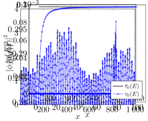
Figure 7: Convergence of $\tau_{0}(E)$ to $\bar{\tau}_{0}(E)$. Parameter values: $W=10^{4}$, $\expectationvalue{\epsilon}=1$, $E=0$ and $\gamma=0.25$.

$$\lim\limits_{N\rightarrow\infty}\int_{0}^{\pi}du\frac{g(u)}{1+h(u)\sin[2uN+r(u)]}=\int_{0}^{\pi}du\frac{g(u)}{\sqrt{1-h^{2}(u)}}.$$ (70)

Converting the integral in Eq. (69) back from $q$ to $k$ and then substituting $\frac{1}{\sqrt{1-R^{2}(q_{\mathbf{k}})}}=\frac{|A(q_{\mathbf{k}})|^{2}+|B(q_{\mathbf{k}})\sin q_{\mathbf{k}}|^{2}}{2\imaginary[A(q_{\mathbf{k}})B^{*}(q_{\mathbf{k}})]\sin q_{\mathbf{k}}}$ we have,

$$\bar{\tau}_{0}(E) =\frac{8\gamma^{2}}{\pi}\int_{0}^{\pi}d\mathbf{k}\frac{\sin q_{\mathbf{k}}}{2\imaginary[A(q_{\mathbf{k}})B^{*}(q_{\mathbf{k}})]}$$ (71)

$$=\frac{4}{\pi}\int_{0}^{\pi}d\mathbf{k}\bar{F}^{o}(q_{\mathbf{k}}).$$ (72)

We show in Fig. (7) the convergence of $\tau_{0}(E)$ to $\bar{\tau}_{0}(E)$ as $L$ is increased.