Learning from Linear Algebra: A Graph Neural Network Approach to Preconditioner Design for Conjugate Gradient Solvers

Abstract

Large linear systems are ubiquitous in modern computational science. The main recipe for solving them is iterative solvers with well-designed preconditioners. Deep learning models may be used to precondition residuals during iteration of such linear solvers as the conjugate gradient (CG) method. Neural network models require an enormous number of parameters to approximate well in this setup. Another approach is to take advantage of small graph neural networks (GNNs) to construct preconditioners of the predefined sparsity pattern. In our work, we recall well-established preconditioners from linear algebra and use them as a starting point for training the GNN. Numerical experiments demonstrate that our approach outperforms both classical methods and neural network-based preconditioning. We also provide a heuristic justification for the loss function used and validate our approach on complex datasets.

1 Introduction

Modern computational science and engineering problems are based on partial differential equations (PDEs). The lack of analytical solutions for typical engineering problems (heat transfer, fluid flow, structural mechanics, etc.) leads researchers to use advances in numerical analysis. Any numerical method for solving PDEs results in a system of linear equations $Ax=b,\,\,A\in\mathbb{R}^{n\times n}$,  $x\in\mathbb{R}^{n}$ and $b\in\mathbb{R}^{n}$. All these systems are usually sparse, meaning that the number of non-zero elements is $\ll n$.

Typically, the application of PDEs produces large linear systems and therefore poses significant computational challenges. This large linear systems are solved by methods that are based on searching for the solution in a Krylov subspace $\mathcal{K}_{r}(A,b)=\text{span}\{b,~{}Ab,~{}A^{2}b,\dots,~{}A^{r-1}b\}.$

The conjugate gradient (CG) is one of these methods. It can be used to solve large sparse systems, especially those with symmetric and positive definite matrices. CG has a well-established convergence theory and convergence guarantees for any symmetric matrix. However, the convergence rate of CG is bounded by $\sqrt{\kappa(A)}$. The condition number $\kappa(A)$ of symmetric positive definite (SPD) matrix $A$, defined in $2\text{-norm}$, is a ratio between maximum and minimum eigenvalues $\kappa(A)=\lambda_{\max}\big{/}\lambda_{\min}$.

Real-world applications with non-smooth high-contrast coefficient functions and/or high-dimensional linear systems separate eigenvalues and results into ill-conditioned problems. Decades of research in numerical linear algebra have been devoted to constructing preconditioners $P$ for ill-conditioned $A$ to improve the condition number in form (for left-preconditioned systems) $\kappa(P^{-1}A)\ll\kappa(A)$.

The well-designed preconditioner should tend to approximate $A$, be easily invertible and be sparse. The construction of a preconditioner is typically a trade-off between the quality of the approximation and the cost of storage/inversion of the preconditioner Saad (2003).

Recent papers on the application of neural networks to speed up iterative solvers include usage of neural operators as nonlinear preconditioner functions Rudikov et al. (2024); Shpakovych (2023) or within a hybrid approach to address low-frequencies Kopaničáková and Karniadakis (2024); Cui et al. (2022) and learning preconditioner decomposition with graph neural networks (GNN) Li et al. (2023); Häusner et al. (2023).

We suggest a GNN-based construction of preconditioners that produce better preconditioners than their classical analogous. Our contributions are as follows:

• We propose a novel scheme for preconditioner design based on learning correction for well-established preconditioners from linear algebra with the GNN.

• We suggest a novel understanding of the loss function used with accent on low-frequencies and provide experimental justification for the understanding of learning with such.

• We propose a novel approach for dataset generation with a measurable complexity metric that addresses real-world problems.

• We provide extensive studies with varying matrix sizes and dataset complexities to demonstrate the superiority of the proposed approach and loss function over classical preconditioners.

2 Neural design of preconditioner

Problem statement

We consider systems of linear algebraic equations from discretization of differential operators $Ax=b$ formed with a symmetric positive definite (SPD) matrices $A\succ 0$. One can use Gaussian elimination of complexity $\mathcal{O}(n^{3})$ to solve small linear systems, but not real-world problems that produce large systems. The CG iterative solver is well-suited for solving large linear systems with SPD matrices, but the CG converges poorly for ill-conditioned systems when $\kappa(A)$ is big.

Preconditioned linear systems

For the SPD linear system, one can form the preconditioner in form of Choletsky decomposition Trefethen and Bau (2022) $P=LL^{\top}$ with sparse $L$, to obtain preconditioned linear system $P^{-1}Ax=P^{-1}b$. If one knows sparsity pattern of $A$, then possible options are incomplete LU decomposition (ILU) Saad (2003): (i) with $p$-level of fill-in denoted as ILU($p$) and (ii) ILU decomposition with threshold with $p$-level of fill-in denoted as ILUt($p$).

Preconditioners with neural networks

Our final goal is to find such decomposition that $\kappa((L(\theta)L(\theta)^{\top})^{-1}A)\ll\kappa((LL^{\top})^{-1}A)\ll\kappa(A)$, where $L$ is classical numerical ILU decomposition and $L(\theta)=\mathcal{F}(A)$ is an approximated decomposition with some function $\mathcal{F}$. Several papers Li et al. (2023); Häusner et al. (2023) suggest to use GNN as function $\mathcal{F}$ to minimize a certain loss function:

$$L(\theta)=\text{GNN}(\theta,A,b)\,.$$ (1)

Loss function

The key question is which objective function to minimize in order to construct a preconditioner. A natural choice which is also used in Häusner et al. (2023) is:

$$\min\big{\|}P-A\big{\|}_{F}^{2}.$$ (2)

By design, this objective minimizes high-frequency components (large eigenvalues), which is not desired. The most important are low-frequency components (small eigenvalues) since they correspond to differentiating phenomenon, when high-frequency comes from discretization methods. We suggest to use $A^{-1}$ as a weight to the previous optimization objective to take into account low-frequency since $\lambda(A)=\lambda^{-1}(A^{-1})$:

$$\min\big{\|}(P-A)A^{-1}\big{\|}^{2}_{F}$$ (3)

Let us rewrite this objective with Hutchinson’s estimator Hutchinson (1989):

$$\big{\|}\big{(}P-A\big{)}A^{-1}\big{\|}^{2}_{F}=\big{\|}PA^{-1}-I\big{\|}_{F}^{2}=\operatorname{Tr}\Big{(}(PA^{-1}-I)^{\top}(PA^{-1}-I)\Big{)}\\ =\mathbb{E}_{\varepsilon}\Big{[}\varepsilon^{\top}(PA^{-1}-I)^{\top}(PA^{-1}-I)\varepsilon\Big{]}=\mathbb{E}_{\varepsilon}\big{\|}(PA^{-1}-I)\varepsilon\big{\|}_{2}^{2},\quad\varepsilon\sim\mathcal{N}(0,1).$$ (4)

Assume we have a dataset of linear systems $A_{i}x_{i}=b_{i}$, then the training objective with $\varepsilon=b_{i},~{}P=L(\theta)L(\theta)^{\top}$ and $A^{-1}_{i}b_{i}=x_{i}$ becomes:

$$\mathcal{L}=\frac{1}{N}\sum_{i=1}^{N}\big{\|}L(\theta)L(\theta)^{\top}x_{i}-b_{i}\big{\|}_{2}^{2}$$ (5)

This loss function previously appeared in related research Li et al. (2023) but with understanding of inductive bias from PDE data distribution. In experiment section we evidence our hypothesis, that loss (5) indeed mitigate low-frequency components.

3 Learn correction for ILU

Our main goal is to construct preconditioners that will reduce condition number of a SPD matrix greater, than classical preconditioners with the same sparisy pattern. We work with SPD matrices so ILU, ILU($p$) and ILUt($p$) results in incomplete Choletsky factorization IC, IC($p$) and ICt($p$).

3.1 Graph neural network with preserving sparsity pattern

Following the idea from Li et al. (2023), we use of GNN architecture Zhou et al. (2020) to preserve the sparsity pattern and predict the lower triangular matrix to create a preconditioner in a form of IC decomposition.

The duality between sparse matrices and graphs is used to obtain vertices and edges, such as $Ax=b\rightarrow\mathcal{G}=(\mathcal{V},\mathcal{E})$, where $a_{i,j}=e_{i,j}\in\mathcal{E},b_{i}=v_{i}\in\mathcal{V}$. The original GNN architecture from Li et al. (2023):

• First step is to use node and edge encoders to increase their dimensionality with multi-layer perceptrons (MLPs): $v_{i}=\text{MLP}_{v}(v_{i}),e_{i,j}=\text{MLP}_{e}(e_{i,j})$.

• Then the encoded graph is processed with $T$ rounds of message passing Brandstetter et al. (2022) ($t=1,\dots,T$) to transfer information between vertices and edges. During a single round, we update vertices with $v_{i,t+1}=\text{MLP}_{mp,v}(v_{i,t},\sum_{j}e_{i,j,t}v_{j,t})$, and then update the edges with $e_{i,j,t+1}=\text{MLP}_{mp,e}(e_{i,j,t},v_{i,t+1}v_{j,t+1}),\,\,\text{for}\,\,i\neq j$.

• Next step is to decode the lower triangular matrix while preserving the information in the upper triangular part of the matrix. To do this we average the bidirectional edges, decode them with MLP and then zero out the upper triangular part: $e_{i,j,T}=\big{(}e_{i,j,T}+e_{j,i,T}\big{)}/2$ and $L_{i,j|i\leq j}=\text{MLP}_{\text{decod}}(e_{i,j,T}),L_{i,j|i>j}=0$.

• After all round of message passing the diagonal of the decomposition inherited as the diagonal from original matrix to ensure SPD property in resulting decomposition $\text{diag}(L(\theta)):=\sqrt{\text{diag}(A)}$.

• Finally, we assemble preconditioners in a form of Choletsky decomposition $P:=L(\theta)L(\theta)^{\top}$.

3.2 PreCorrector

Instead of passing left-hand side matrix $A$ as an input to GNN (1), we propose: (i) to pass $L$ from IC decomposition to the GNN and (ii) to train GNN to predict a correction for this decomposition (Figure 1). We name our approach as PreCorrector (Preconditioner Corrector):

$$L(\theta)=L+\alpha\cdot\text{GNN}(\theta,L,b).$$ (6)

The correction coefficient $\alpha$ is also a learning parameter that is updated during gradient descent training. At the beginning of training, we set $\alpha=0$ to ensure that the first gradient updates come from pure IC factorization. Since we already start with a good initial guess, we observed that pinning the diagonal is redundant and limits the PreCorrector training. Moreover, GNN in (6) takes as input the lower-triangular matrix $L$ from IC instead of $A$, so we are not anchored to a single specific sparse pattern of $A$ and we can: (i) omit half of the graph and speed up the training process and (ii) use different sparsity patterns. In experiment section we show that the proposed approach with input $L$ from IC(0) and ICt(1) indeed produce better preconditioners compared to classical IC(0) and ICt(1).

Figure 1: PreCorrector scheme that starts with IC(0) decomposition. (a) Start with linear system $Ax=b$. (b) Obtain $L_{0}$ from IC(0) decomposition. (c) Input $L_{0}$ and $b$ to GNN. (d) Calculate $L(\theta)$ with (6) and construct preconditioner in form of IC. (Very right picture) Note that obtained preconditioner in form of IC(0) decomposition can be stored as initial matrix $A$.

4 Dataset

We want to validate our approach on the data that addresses real-world problems. We consider a 2D diffusion equation:

$$\begin{split}-&\nabla\cdot\big{(}k(x)\nabla u(x)\big{)}=f(x),~{}\text{in}~{}\Omega\\ &u(x)\Big{|}_{x\in\partial{\Omega}}=0\end{split}\,\,\,,$$ (7)

where $k(x)$ is a diffusion coefficient, $u(x)$ is a solution and $f(x)$ is a forcing term.

The diffusion equation is chosen because of its frequent appearance in many engineering applications, such as: composite modeling Carr and Turner (2016), geophysical surveys Oristaglio and Hohmann (1984), fluid flow modeling Muravleva et al. (2021). In these cases, the coefficient functions are discontinuous, i.e. they change rapidly within neighbouring cells. An example of this is the flow of fluids of different viscosities.

We propose to measure the complexity of the dataset by contrast of the coefficient function:

$$\text{contrast}=\exp\big{(}\max k(x)-\min k(x)\big{)},\quad x\in\Omega.$$ (8)

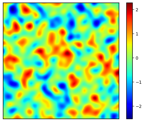
Figure 2: The Gaussian random field coefficient $k(x)$ for grid $128\times 128$ and variance $0.7$.

The higher the contrast (8), the more iterations are required in CG to achieve the desired tolerance, and the more complex the dataset. Condition number of resulting linear system depends on grid and the contrast, but usually high contrast is not taken into account.

As a coefficient function in diffusion equation we use Gaussian random field (GRF) with efficient realization in parafields library (Figure 2). The forcing term $f$ is sampled from the standard normal distribution and each PDE is discretized using the 5-point finite difference method.

We generate four different datasets with different complexity for each grid value from $\{32,64,128\}$. Contrast in datasets is controlled with a variance in coefficient function GRF and takes value in $\{0.1,0.5,0.7\}$. Datasets are discretized with finite difference method with five-point stencil. One can find greater details about datasets in Appendix A.1.

Table 1: Comparison of the PreCorrector with classical preconditioners on datasets $\text{Diff}_{0.1}$, $\text{Diff}_{0.5}$ and $\text{Diff}_{0.7}$. PreCor stands for PreCorrector.

		Grid $32\times 32$			Grid $64\times 64$			Grid $128\times 128$
Dataset	Method	$10^{-3}$	$10^{-6}$	$10^{-9}$	$10^{-3}$	$10^{-6}$	$10^{-9}$	$10^{-3}$	$10^{-6}$	$10^{-9}$
$\text{Diff}_{0.1}$	$\text{IC}(0)$	33	43	55	66	85	108	133	170	216
	PreCor$\big{[}\text{IC}(0)\big{]}$	22	30	37	34	44	57	52	66	84
	$\text{ICt}(1)$	21	27	35	40	52	66	81	104	131
	PreCor$\big{[}\text{ICt}(1)\big{]}$	16	21	27	24	31	41	39	50	64
$\text{Diff}_{0.5}$	$\text{IC}(0)$	38	49	62	75	95	122	149	194	246
	PreCor$\big{[}\text{IC}(0)\big{]}$	26	34	43	40	52	67	68	89	115
	$\text{ICt}(1)$	23	29	38	45	58	75	91	117	150
	PreCor$\big{[}\text{ICt}(1)\big{]}$	17	23	29	28	36	47	47	61	77
$\text{Diff}_{0.7}$	$\text{IC}(0)$	40	51	66	80	102	130	160	209	261
	PreCor$\big{[}\text{IC}(0)\big{]}$	27	36	46	45	59	76	76	99	125
	$\text{ICt}(1)$	24	31	40	48	61	79	97	128	159
	PreCor$\big{[}\text{ICt}(1)\big{]}$	19	25	31	30	40	51	53	69	88

5 Experiments

In our approach, we use both IC(0) and ICt(1) as starting points for training. In the next section, we will use following notations:

• IC(0), ICt(1), ICt(5) are classical preconditioners from linear algebra with a corresponding level of fill-in $k$.

• PreCorrector$\big{[}$IC(0)$\big{]}$ and PreCorrector$\big{[}$ICt(1)$\big{]}$ are the proposed approach with corresponding preconditioner as input.

The complexity of solving sparse linear systems with matrices in form of Choletsky decomposition defined by the number of non-zero elements $\mathcal{O}(\text{nnz})$. This value also illustrates the storage complexity and the complexity of the preconditioner construction.

The construction of a classical preconditioner for large linear systems may also be a problem so we estimated time of IC preconditioner construction and inference time of the proposed PreCorrector. To construct classical preconditioners we use an efficient realization of those in ilupp library Mayer (2007).Precompute time averaged over 200 test samples of $A\in\mathbb{R}^{16\cdot 10^{4}\times 16\cdot 10^{4}}$:

• $5\cdot 10^{-4}$ sec for IC(0).

• $4\cdot 10^{-3}$ sec for ICt(1).

• $8\cdot 10^{-3}$ sec for ICt($5$).

• $1\cdot 10^{-1}$ sec for PreCorrector$\big{[}$IC(0)$\big{]}$ and PreCorrector$\big{[}$ICt(1)$\big{]}$.

5.1 Experiment environment

Each dataset from the Section 4 consists of $1000$ training and $200$ test linear systems. Full datasets are used for experiments unless otherwise stated. We train the neural network model with batch size in $\{8,~{}16\}$, learning rate in $\{10^{-3},~{}5\cdot 10^{-3}\}$ using the Adam optimizer. For a fair comparison, we set the GNN architecture to $5$ message passing rounds and $2$ hidden layers with $16$ hidden features in all MLPs (see Section 3.1) in each experiment. PreCorrector’s training always starts with the parameter $\alpha=0$ in (6). We use a single GPU Nvidia A40 48Gb for training.

5.2 Comparison with classical preconditioners

The proposed approach construct better preconditioner with increasing complexity of linear systems (Table 1). As the variance and/or grid size of the dataset grows, PreCorrector$\big{[}$IC(0)$\big{]}$ preconditioner, made with IC(0) sparsity pattern, outperform the same vanilla preconditioner up to a factor of $3$. This effect is particularly important for memory/efficiency trade-off. If one can afford memory, the PreCorrector$\big{[}$ICt(1)$\big{]}$ preconditioner produces speed-up up to a factor of $2$ compared to ICt(1).

While it is not completely fair to compare results of preconditioners with different densities, we observed that PreCorrector can outperform classical preconditioners with greater nnz values. The PreCorrector$\big{[}$IC(0)$\big{]}$ outperform ICt(1) up to a factor of $1.2-1.5$, meaning we can achieve better approximation $P\approx A$ with less nnz value. Moreover, the effect of the PreCorrector$\big{[}$ICt(1)$\big{]}$ preconditioner is comparable to the ICt(5) preconditioner, which has $1.5$ times larger nnz value than initial matrix $A$ (A.2.

Architecture of the PreCorrector opens for interpretations value of the correction coefficient $\alpha$ in (6). In our experiments, the value of $\alpha$ is always negative and its values are clustered in intervals $[-0.135,-0.095]$ and $[-0.08,-0.04]$. One can find greater details about values of coefficient $\alpha$ in Appendix A.3.

Figure 3: Test loss during training of PreCorrector$\big{[}$IC(0)$\big{]}$ on the $\text{Diff}_{0.5}$ dataset

5.3 Loss function

The equivalence of (3) and (5) allows to avoid explicit inverse materialization and provides maximum complexity of the matrix-vector product in the loss during training. Now recall that $A$ comes from the 5-point finite difference discretization of the diffusion equation 4. $A$ tends to a diagonal matrix with $n\rightarrow\infty$ and we can assume that $A$ is a diagonal matrix for sufficiently large linear systems. Then minimizing a matrix product between the preconditioner and $A^{-1}$ in (3) makes the eigenvalues tend to $1$.

As stated in Section 2, one should focus on approximation of low frequency components. In the Table 2 we can see that the proposed loss does indeed reduce the distance between extreme eigenvalues compared to IC(0). Moreover, the gap between the extreme eigenvalues is covered by the increase in the minimum eigenvalue, which supports the hypothesis of low frequency cancellation. Maximum eigenvalue also grows but with way less order of magnitude.

At the same time, preconditioner trained with the loss function (2) without $A^{-1}$ provides worse effect on the CG and suffers to produce the same effect on spectrum (Table 3).

Table 2: Condition number, spectrum and value of loss 3 for a sampled model from dataset $\text{Diff}_{0.7}$ with grid $64\times 64$.

Matrix	$\kappa(P^{-1}A)$	$\lambda_{\text{min}}$	$\lambda_{\text{max}}$	$\big{\|}LL^{\top}A^{-1}-I\big{\|}^{2}_{F}$
$A$	$15888$	$21.7043$	$344834.41$	—
$\big{(}L_{0}L_{0}^{\top}\big{)}^{-1}A$	$270$	$0.0055$	$1.22$	$69445$
$\big{(}L(\theta)L(\theta)^{\top}\big{)}^{-1}A$	$55$	$0.2324$	$7.21$	$447$

Table 3: Loss comparison. Number of CG iterations on the dataset $\text{Diff}_{0.7}$ with grid $32\times 32$. ¹Condition number and eigenvalues are calculated on a single sampled linear system.

Loss	$10^{-3}$	$10^{-6}$	$10^{-9}$	$\kappa(P^{-1}A)^{1}$	$\lambda_{\text{min}}^{1}$	$\lambda_{\text{max}}^{1}$
2	$45$	$58$	$74$	$88$	$0.0169$	1.17
3 $(\textbf{Ours})$	27	36	49	25	0.2889	$3.92$

5.4 Generalization to different grids and datasets

We also observe a good generalization of our approach when transferring our preconditioner between grids and datasets (Figure 4). The transfer between datasets of increasing and decreasing complexity does not lead to a loss of quality. This means that we can train the model with simple PDEs and then use it with complex ones for inference. If we fix the complexity of the dataset and try to transfer the learned model to other grids, we observe a loss of quality of only about $10\%$.

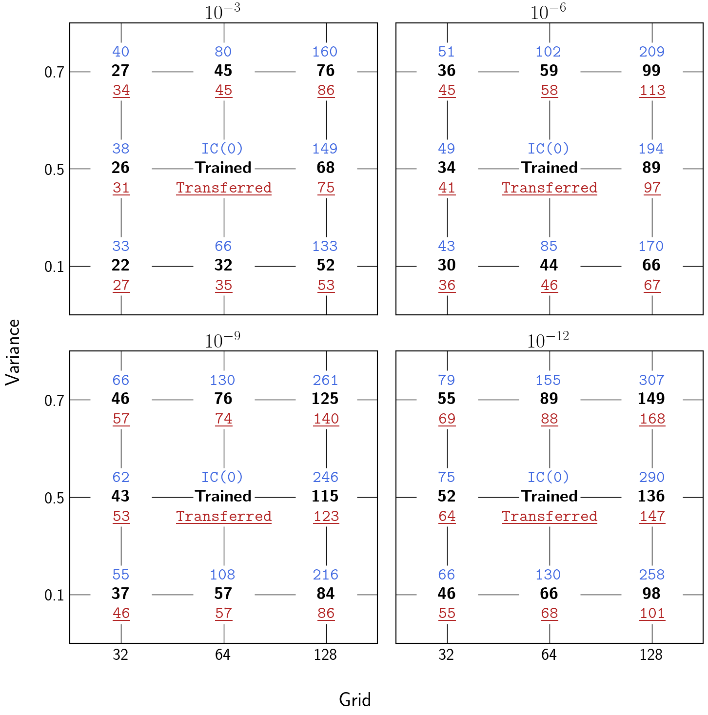
Figure 4: The proposed approach generalizes on unseen datasets. Values are number of CG iterations to achieve required tolerance, which specified in the title of each plot. Blue – IC(0) is used as preconditioner. Black – PreCorrector$\big{[}$IC(0)$\big{]}$; trained and inferenced on the same dataset. Red – PreCorrector$\big{[}$IC(0)$\big{]}$; trained on the dataset $\text{Diff}_{0.5}$ with grid $64\times 64$; inferenced on the dataset, that is described by axes values.

6 Related work

In this section, we discuss the most important research on learning-based preconditioners that helped us to properly organise our work. While there is a dozen of different preconditioners in linear algebra, for example Saad (2003); Axelsson (1996): block Jacobi preconditioner, Gauss-Seidel preconditioner, sparse approximate inverse preconditioner, algebraic multigrid methods, etc. The choice of preconditioner depends on the specific problem and practitioners often rely on a combination of theoretical understanding and numerical experimentation to select the most effective preconditioner. Even a brief description of all of them is beyond the scope of a single research paper. One can refer to related literature for more details

The authors of Li et al. (2023) present a novel approach to preconditioner design using GNN and a new loss function that incorporates inductive bias from PDE data distributions. This learning-based method aims to approximate the matrix factorization and use it as a preconditioner, exploiting the common sparsity pattern between the left-hand side $A$ and the output of GNN. The proposed approach is shown to be more efficient than classical linear algebra preconditioners when their pre-computation time is much higher than GNN inference.

The recent FCG-NO Rudikov et al. (2024) approach to solving linear systems of PDEs by combining neural operators with the conjugate gradient method acts as a nonlinear preconditioner for the flexible conjugate gradient method. This approach exploits the strengths of both neural networks and the FCG method to create a computationally efficient, data-driven approach. The authors use the FCG with a proven convergence bound for a nonlinear preconditioner and use it as a training loss.

A paper Kopaničáková and Karniadakis (2024) introduces a novel class of hybrid preconditioners for solving parametric linear systems of equations by combining DeepONet with standard iterative methods. The proposed framework consists of two approaches: direct preconditioning (DP) and trunk basis (TB), which use DeepONet to address low-frequency error components and conventional iterative methods to mitigate high-frequency error components.

The in Zhang et al. (2022) proposed HINTS method combines traditional relaxation methods with the Deep Operator Network (DeepONet) to solve differential equations more efficiently and accurately. It targets different regions of the spectrum, ensuring a uniform convergence rate and exceptional performance. Authors reported that HINTS is fast, accurate and applicable to various differential equations, domains, discretizations and can be transferred to different discretizations.

7 Conclusion and further work

We proposed a novel learnable approach for preconditioner construction – PreCorrector. PreCorrector successfully demonstrated the potential of neural networks in the construction of effective preconditioners for solving linear systems, that can outperform classical numerical preconditioners. By learning the corrections to classical preconditioners, we developed a novel approach that combines the strengths of traditional preconditioning techniques with the flexibility of neural networks. We suggest that there exists a learnable transformation that will be universal for different sparse matrices for construction of ILU decomposition that will significantly reduce $\kappa(A)$.

Our observation about approximation of low-frequency components in the used loss function lacks theoretical analysis. Moreover we did not found any traces of the seeking relationship in the specialized literature. We suppose that this loss analysis is the key ingredient for successful learning general form transformation.

We also suggested a complexity metric for our dataset and showed superiority of the PreCorrector approach over classical preconditioners of ILU class on complex datasets.

Further work may be summarized as follows:

• Theoretical investigation of the used loss function.

• Analysis of possible variations of the target objective in other norms.

• Generalization of the PreCorrector to transformation in the space of sparse matrices with general sparsity pattern.

Appendix A Appendix

A.1 Details on training data

Table 4: Dataset specification.

Name	Grid	Variance	Min contrast	Mean contrast	Max contrast
$\text{Diff}_{0.1}$	$32$	$0.1$	$5$	$7$	$11$
	$64$		$5$	$8$	$12$
	$128$		$6$	$8$	$14$
$\text{Diff}_{0.5}$	$32$	$0.5$	$36$	$86$	$179$
	$64$		$45$	$103$	$200$
	$128$		$50$	$116$	$297$
$\text{Diff}_{0.7}$	$32$	$0.7$	$180$	$277$	$697$
	$64$		$200$	$318$	$742$
	$128$		$300$	$426$	$798$

Table 5: Size of linear systems and number of nonzero elements (nnz) for different grids and matrices.

	Grid $32\times 32$		Grid $64\times 64$		Grid $128\times 128$
Matrix	Size	nnz, $\%$	Size	nnz, $\%$	Size	nnz, $\%$
$A$	$1024$	0.4761	$4096$	0.1205	$16384$	0.0303
$L$ from IC($0$)		0.2869		0.0725		0.0182
$L$ from ICt($1$)		0.3785		0.0961		0.0242
$L$ from ICt($5$)		0.7547		0.1920		0.0485

A.2 Additional experiments with ICt($5$) preconditioner

Table 6: Comparison of the PreCorrector$\big{[}$ICt(1)$\big{]}$ and ICt(5) preconditioners on datasets $\text{Diff}_{0.5}$ and $\text{Diff}_{0.7}$. PreCor stands for PreCorrector.

		Grid $32\times 32$			Grid $64\times 64$			Grid $128\times 128$
Dataset	Method	$10^{-3}$	$10^{-6}$	$10^{-9}$	$10^{-3}$	$10^{-6}$	$10^{-9}$	$10^{-3}$	$10^{-6}$	$10^{-9}$
$\text{Diff}_{0.5}$	$\text{ICt}(5)$	11	15	20	22	29	37	47	61	78
	PreCor$\big{[}\text{ICt}(1)\big{]}$	17	23	29	28	36	47	47	61	77
$\text{Diff}_{0.7}$	$\text{ICt}(5)$	12	15	20	23	30	39	49	66	81
	PreCor$\big{[}\text{ICt}(1)\big{]}$	19	25	31	30	40	51	53	69	88

A.3 Details about correction coefficient $\alpha$

Table 7: Values of the learned coefficient alpha from 6.

	Grid $32\times 32$		Grid $64\times 64$		Grid $32\times 128$
PDE	IC(0)	ICt(1)	IC(0)	ICt(1)	IC(0)	ICt(1)
Poisson	$-0.1344$	$-0.0640$	$-0.1226$	$-0.0640$	$-0.0968$	$-0.0964$
$\text{Diff}_{0.1}$	$-0.0695$	$-0.0541$	$-0.1175$	$-0.0771$	$-0.0792$	$-0.0648$
$\text{Diff}_{0.5}$	$-0.0660$	$-0.0557$	$-0.0712$	$-0.0441$	$-0.0713$	$-0.0520$
$\text{Diff}_{0.7}$	$-0.0618$	$-0.0455$	$-0.0769$	$-0.0519$	$-0.0811$	$-0.0374$

References

- Saad (2003) Yousef Saad. Iterative methods for sparse linear systems. SIAM, 2003.
- Rudikov et al. (2024) Alexander Rudikov, Vladimir Fanaskov, Ekaterina Muravleva, Yuri M Laevsky, and Ivan Oseledets. Neural operators meet conjugate gradients: The fcg-no method for efficient pde solving. arXiv preprint arXiv:2402.05598, 2024.
- Shpakovych (2023) Maksym Shpakovych. Neural network preconditioning of large linear systems. PhD thesis, Inria Centre at the University of Bordeaux, 2023.
- Kopaničáková and Karniadakis (2024) Alena Kopaničáková and George Em Karniadakis. Deeponet based preconditioning strategies for solving parametric linear systems of equations. arXiv preprint arXiv:2401.02016, 2024.
- Cui et al. (2022) Chen Cui, Kai Jiang, Yun Liu, and Shi Shu. Fourier neural solver for large sparse linear algebraic systems. Mathematics, 10(21):4014, 2022.
- Li et al. (2023) Yichen Li, Peter Yichen Chen, Tao Du, and Wojciech Matusik. Learning preconditioners for conjugate gradient pde solvers. In International Conference on Machine Learning, pages 19425–19439. PMLR, 2023.
- Häusner et al. (2023) Paul Häusner, Ozan Öktem, and Jens Sjölund. Neural incomplete factorization: learning preconditioners for the conjugate gradient method. arXiv preprint arXiv:2305.16368, 2023.
- Trefethen and Bau (2022) Lloyd N Trefethen and David Bau. Numerical linear algebra. SIAM, 2022.
- Hutchinson (1989) Michael F Hutchinson. A stochastic estimator of the trace of the influence matrix for laplacian smoothing splines. Communications in Statistics-Simulation and Computation, 18(3):1059–1076, 1989.
- Zhou et al. (2020) Jie Zhou, Ganqu Cui, Shengding Hu, Zhengyan Zhang, Cheng Yang, Zhiyuan Liu, Lifeng Wang, Changcheng Li, and Maosong Sun. Graph neural networks: A review of methods and applications. AI open, 1:57–81, 2020.
- Brandstetter et al. (2022) Johannes Brandstetter, Daniel Worrall, and Max Welling. Message passing neural pde solvers. arXiv preprint arXiv:2202.03376, 2022.
- Carr and Turner (2016) EJ Carr and IW Turner. A semi-analytical solution for multilayer diffusion in a composite medium consisting of a large number of layers. Applied Mathematical Modelling, 40(15-16):7034–7050, 2016.
- Oristaglio and Hohmann (1984) Michael L Oristaglio and Gerald W Hohmann. Diffusion of electromagnetic fields into a two-dimensional earth: A finite-difference approach. Geophysics, 49(7):870–894, 1984.
- Muravleva et al. (2021) Ekaterina A Muravleva, Dmitry Yu Derbyshev, Sergei A Boronin, and Andrei A Osiptsov. Multigrid pressure solver for 2d displacement problems in drilling, cementing, fracturing and eor. Journal of Petroleum Science and Engineering, 196:107918, 2021.
- Mayer (2007) Jan Mayer. A multilevel crout ilu preconditioner with pivoting and row permutation. Numerical Linear Algebra with Applications, 14(10):771–789, 2007.
- Axelsson (1996) Owe Axelsson. Iterative solution methods. Cambridge university press, 1996.
- Zhang et al. (2022) Enrui Zhang, Adar Kahana, Eli Turkel, Rishikesh Ranade, Jay Pathak, and George Em Karniadakis. A hybrid iterative numerical transferable solver (hints) for pdes based on deep operator network and relaxation methods. arXiv preprint arXiv:2208.13273, 2022.