Massive MIMO-ISAC System With
1-Bit ADCs/DACs

Abstract

This paper investigates a hardware-efficient massive multiple-input multiple-output integrated sensing and communication (MIMO-ISAC) system with 1-bit analog-to-digital converters (ADCs)/digital-to-analog converters (DACs). The proposed system, referred to as 1BitISAC, employs 1-bit DACs at the ISAC transmitter and 1-bit ADCs at the sensing receiver, achieving significant reductions in power consumption and hardware costs. For such kind of systems, two 1BitISAC joint transceiver designs, i.e., i) quality of service constrained 1BitISAC design and ii) quality of detection constrained design, are considered and the corresponding problems are formulated. In order to address these problems, we thoroughly analyze the radar detection performance after 1-bit ADCs quantization and the communication bit error rate. This analysis yields new design insights and leads to unique radar and communication metrics, which enables us to simplify the original problems and employ majorization-minimization and integer linear programming methods to solve the problems. Numerical results are provided to validate the performance analysis of the proposed 1BitISAC and to compare with other ISAC configurations. The superiority of the proposed 1BitISAC system in terms of balancing ISAC performance and energy efficiency is also demonstrated.

I Introduction

Wireless communication and radar are two major applications of electromagnetic (EM) waves, where wireless communication uses EM waves to convey information, while radar utilizes EM waves to detect, estimate, and track targets. Although wireless communication and radar share many similarities, they have been developed independently over the past few decades [2]. Recently, future 5G-Advanced and 6G, are envisioned to simultaneously provide wireless communication services and environment-aware sensing [3]. This demand has spurred the research into integrated sensing and communications (ISAC), where communication and radar sensing functions are realized using a common hardware platform and waveform, opening a new era of jointly researching communication and radar technologies [4]. Benefiting from the ability to achieve spectrum sharing, reduce hardware requirements, and realize integration gains, ISAC has become a key technology in the next-generation wireless networks [5].

I-A Related Works

In general, the design approaches of ISAC can be roughly categorized into three types: communication-centric design (CCD), radar-centric design (RCD), and dual-function waveform design (DFWD).

i) Communication-Centric Design: The CCD aims to directly exploit the classical communication standards (waveforms) or perform some modifications to achieve the radar sensing as a secondary functionality [6, 7, 8, 9]. For example, the authors in [6] utilize the Wi-Fi standard to achieve indoor sensing, where indoor sensing is realized by carefully modifying the Wi-Fi standard to extract indoor environment information. Besides, the authors in [7] discuss using the IEEE 802.11p standard to support vehicular environment sensing. In addition to modifying IEEE 802.11p, modifications to the IEEE 802.11ad standard have been presented in [8] to enhance sensing capabilities in vehicular environment.

ii) Radar-Centric Design: Similar to CCD, the RCD aims to embedded communication symbols into existing radar waveforms to achieve the communication as a secondary functionality [10, 11, 12]. For instance, the authors in [10] propose to embed binary phase-shift keying (PSK) symbols into linear frequency modulation (LFM) waveforms. As a further step, it is proposed in [11] to embed PSK symbols into a frequency-hopping (FH) waveform, where the embedding strategy of communication symbols is carefully studied. To further enhance the communication rate, an innovative approach that embeds quadrature amplitude modulation signals into the sidelobes of radar waveforms has been developed in [12].

iii) Dual-Function Waveform Design: The CCD and RCD prioritize either communication or radar sensing capabilities in the ISAC system, treating the other functionality as secondary, which leads to performance losses on the secondary functionality. To overcome this drawback and achieve enhanced and balanced ISAC performance, the DFWD approaches have been investigated in [13, 14, 15, 16, 17, 18, 19, 20]. Specifically, DFWD aims to design waveforms (beamformers) that simultaneously optimize both radar sensing and communication metrics. Notably, common radar sensing metrics include radar signal-to-interference-plus-noise ratio (SINR) [13, 14], beampattern mean squared error (MSE) [15, 16], Cramér-Rao Bound (CRB) [17, 18], and mutual information [19, 20]. Additionally, communication metrics encompass communication achievable rate [19], communication user SINR [15], communication minimum MSE (MMSE) [20], constructive interference (CI) [16]. The resultant DFWD problem can be tackled using numerical optimization methods or machine learning.

I-B Motivations and Contributions

In the upcoming 5G-Advanced and 6G, massive multiple-input multiple-output (MIMO) is a compelling technology that supports hundredfold communication throughput improvements and achieves millimeter-level sensing. Therefore, synergizing ISAC with massive MIMO technology has become increasingly promising for achieving high-throughput communication and higher-precision radar sensing. However, directly extending the aforementioned approaches [13, 14, 15, 16, 17, 18, 19, 20] to massive MIMO ISAC systems presents significant challenges. Specifically, previous studies assume ISAC is equipped with a fully-digital beamforming (FD-BF) architecture, where each antenna is connected to one RF chain. The large number of antennas in massive MIMO ISAC systems necessitates a corresponding scale-up of RF chains, leading to prohibitively high power consumption and hardware costs. Therefore, investigating energy and hardware efficient solutions for massive MIMO ISAC systems has become imperative.

To tackle this challenge, the low-resolution massive MIMO (LowRes-MIMO) architecture has been proposed, where the RF chains utilize few-bit ADCs/DACs to significantly reduce both hardware cost and power consumption. LowRes-MIMO was first introduced in communication areas [21, 22, 23, 24, 25, 26] and has received significant research attention. Subsequently, it has been extended to radar applications [27, 28, 29, 30, 31, 32, 33]. Given the successful application of LowRes-MIMO in both communication and radar areas, researchers propose achieving massive MIMO ISAC by employing LowRes-MIMO architecture [34, 35]. Specifically, prior work conducted in [34] designs an ISAC system with 1-bit DACs by minimizing the CRB while guaranteeing the MMSE in communications. Following this, the authors in [35] propose an ISAC system with 1-bit DACs, designed by minimizing the weighted of radar beampattern MSE and communication MMSE.

Although [34, 35] achieve satisfactory ISAC performance, they have the following two limitations: i) The aforementioned works [34, 35] focus solely on the ISAC transmit design with 1-bit DACs. It is widely acknowledged that joint transceiver design can enhance ISAC performance. However, if the ISAC sensing receiver adopts 1-bit ADCs, the sensing performance may be adversely affected by quantization. This raises a critical question: “How much will 1-bit ADCs impact the radar sensing performance in ISAC systems?” ii) The aforementioned works [34, 35] measure communication performance using MMSE, which guarantees performance by alleviating multi-user interference (MUI). However, when the ISAC transmitter is equipped with 1-bit DACs, the flexibility for managing MUI becomes limited. This raises another critical question: “Is MMSE effective in measuring communication performance in ISAC systems with 1-bit DACs?”

To answer the above two questions, this paper proposes an ISAC system with 1-bit ADCs/DACs, termed as 1BitISAC, and thoroughly studies the sensing and communication performance based on theoretical analysis and optimizations. The contributions of this work can be summarized as follows:

Firstly, 1BitISAC Performance Analysis. The detection performance of 1BitISAC is comprehensively analyzed, revealing only 1.96dB performance loss caused by 1-bit ADC quantization in 1BitISAC system with massive MIMO. This analysis provides valuable insights for designing 1BitISAC system. Additionally, the BER performance of the considered 1BitISAC is analyzed. This analysis points out that as long as the received signal is pushed into the safe margin, communication BER performance can be guaranteed. This highlights a new perspective on ensuring high quality of service (QoS) communication in 1BitISAC system.

Secondly, Joint Transceiver 1BitISAC Design. Two 1BitISAC designs are proposed in this paper: the QoS-constrained 1BitISAC design and the quality of detection (QoD)-constrained 1BitISAC design. Specifically, the QoS-constrained 1BitISAC design aims to maximize radar detection performance while adhering to communication QoS constraints. Guided by insightful performance analysis, the QoS-constrained 1BitISAC design problem is reformulated into a more tractable form and subsequently solved using a proposed method that combines integer linear programming (ILP) and majorization-minimization (MM). Additionally, we extend the proposed QoS-constrained 1BitISAC design to a QoD-constrained 1BitISAC design, where radar detection performance is constrained while communication QoS is maximized.

Thirdly, Performance Validation and Comparison. Extensive simulation results are provided to verify the performance analysis of 1BitISAC. Additionally, the proposed 1BitISAC system is compared with other ISAC configurations (featuring either 1-bit ADCs or 1-bit DACs) to determine which is more promising for ISAC implementations with massive MIMO. Simulation results demonstrate that the proposed 1BitISAC achieves an effective trade-off between ISAC performance and energy efficiency.

I-C Organization and Notations

Organization: Section II presents the system model of the proposed 1BitISAC. Section III offers a comprehensive performance analysis of 1BitISAC. Section IV formulates a QoS-constrained 1BitISAC design problem and provides its solution. Section V extends to a QoD-constrained 1BitISAC design problem. Finally, Section VI present numerous simulation results and Section VII concludes this work.

Notations: Vectors and matrices are denoted by standard lower case boldface letter ${\bm{a}}$ and upper case boldface letter ${\bm{A}}$, respectively. $\mathbb{C}^{n}$ and $\mathbb{C}^{m\times n}$ denote the $n$-dimensional complex-valued vector space and $m\times n$ complex-valued matrix space, respectively. $(\cdot)^{T}$, $(\cdot)^{H}$, and $(\cdot)^{-1}$ denote the transpose, conjugate-transpose operations, and inversion, respectively. $\Re\{\cdot\}$ and $\Im\{\cdot\}$ denote the real and imaginary part of a complex number, respectively. $\|\cdot\|_{F}$ and $|\cdot|$ denote the Frobenius norm and magnitude, respectively. $\text{Tr}(\cdot)$ denotes the summation of diagonal elements of a matrix. $\mathsf{Diag}(\cdot)$ denotes a diagonal matrix.

II Signal Model

In this section, models for the 1BitISAC system are introduced and problem statements for the 1BitISAC designs are presented.

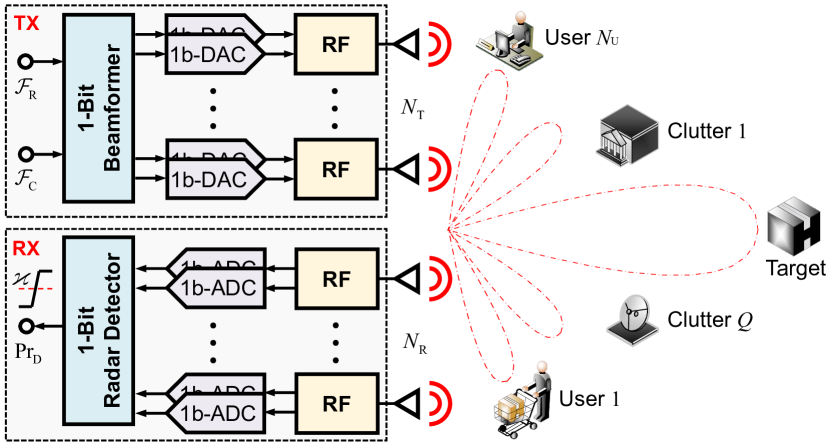
Figure 1: Diagram of the proposed 1BitISAC.

II-A System Model

As shown in Fig. 1, we consider a 1BitISAC scenario consisting of a dual-function BS (DFBS), a target, $Q$ clutter sources, and $N_{\mathrm{U}}$ single-antenna user equipments (UEs). The DFBS simultaneously transmits a dual-function waveform to probe the target of interest and provide communication services to the UEs. The DFBS receives the backscattered signal from the target and clutter sources to detect the target and suppress the clutter sources. We assume the transmitter and receiver of the DFBS are co-located. To reduce hardware costs and power consumption, the DFBS employs 1-bit DACs at its transmitter and 1-bit ADCs at its receiver.

In the 1BitISAC transmitter, according to the radar and communication functions, the communication signal ${\bm{s}}=[s_{1},\cdots,s_{N_{\mathrm{U}}}]^{T}$ is precoded into an unquantized transmit signal ${\bm{x}}_{\mathrm{o}}$ via a beamformer $\mathcal{B}$, i.e., ${\bm{x}}_{\mathrm{o}}=\mathcal{B}({\bm{s}})\in\mathbb{C}^{N_{\mathrm{T}}}$. With 1-bit DACs employed at the transmitter, the baseband signal ${\bm{x}}_{\mathrm{o}}$ is quantized by 1-bit DACs, then the transmit signal can be written as

$${\bm{x}}=\mathcal{Q}_{\text{DAC}}^{\text{1-Bit}}\left({\bm{x}}_{\mathrm{o}}\right)=\mathcal{Q}_{\text{DAC}}^{\text{1-Bit}}\left(\mathcal{B}\left({\bm{s}}\right)\right)\in\mathcal{X}_{\text{DAC}}^{\text{1-Bit}},$$ (1)

where $\mathcal{Q}_{\text{DAC}}^{\text{1-Bit}}(\cdot)$ represents the complex-valued 1-bit DACs quantization operator. The output of $\mathcal{Q}_{\text{DAC}}^{\text{1-Bit}}(\cdot)$ falls within the quantization alphabet $\mathcal{X}_{\text{DAC}}^{\text{1-Bit}}=\left\{\pm\sqrt{\frac{E}{2N_{\mathrm{T}}}},\pm\jmath\sqrt{\frac{E}{2N_{\mathrm{T}}}}\right\}$, where $E$ denotes the transmit power budget.

The above workflow is known as two-stage beamforming-quantized design [36]. Since the 1-bit DAC quantization in (1) introduces non-linear distortion, this beamforming-quantized design typically suffers from severe performance loss [36]. To address this issue, as suggested in [34, 35, 25, 23, 22, 36], we propose to directly design the 1-bit transmit signal ${\bm{x}}$, which will be detailed in Sections IV and V. In the following subsections, we will elaborate on the radar and communication functions.

II-B Radar Model

Suppose there exists a target of interest in the presence of $Q$ clutter sources, located at $\theta_{0}$ and $\theta_{q},\forall q$, respectively. Thus, the echo signals collected by the DFBS receiver can be expressed as

$${\bm{r}}= {\bm{r}}_{\mathrm{T}}+{\bm{r}}_{\mathrm{C}}+{\bm{n}}_{\mathrm{R}}=\underbrace{\gamma_{0}{\bm{G}}_{0}{{\bm{x}}}}_{{\bm{r}}_{\mathrm{T}}}+\sum\limits_{q=1}^{Q}\underbrace{{{\gamma_{q}}{\bm{G}}_{q}{{\bm{x}}}}}_{{\bm{r}}_{\mathrm{C},q}}+{\bm{n}}_{\mathrm{R}}.$$ (2a)

where ${\bm{n}}_{\mathrm{R}}$ is additive white Gaussian noise (AWGN) with ${\bm{n}}_{\mathrm{R}}\sim\left(0,\sigma_{\mathrm{R}}^{2}{\bm{I}}_{N_{\mathrm{R}}}\right)$. $\gamma_{0}$ represents the complex amplitude of target with ${\gamma_{0}}\sim{\mathcal{C}}{\mathcal{N}}\left({0,\varsigma_{0}^{2}}\right)$. Similarly, ${\gamma_{q}}$ denotes the complex amplitude of clutter source $q$ with ${\gamma_{q}}\sim{\mathcal{C}}{\mathcal{N}}\left({0,\varsigma_{q}^{2}}\right),\forall q$, where the DFBS only knows the $\varsigma_{q}^{2}$ without accurate value of ${\gamma_{q}}$. ${\bm{G}}_{0}={{{\bm{g}}}_{\mathrm{R}}}\left({{\theta_{0}}}\right){{\bm{g}}}_{\mathrm{T}}^{T}\left({{\theta_{0}}}\right)$ and ${\bm{G}}_{q}={{{\bm{g}}}_{\mathrm{R}}}\left({{\theta_{q}}}\right){{\bm{g}}}_{\mathrm{T}}^{T}\left({{\theta_{q}}}\right)$ respectively denote the equivalent radar channel for target and clutter $q$. ${\bm{g}}_{\mathrm{T}}(\theta)$ and ${\bm{g}}_{\mathrm{R}}(\theta)$ stand for transmit and receive steering vectors, respectively, given by:

$${\bm{g}}_{\mathrm{T}}(\theta) =\frac{1}{\sqrt{N_{\mathrm{T}}}}\left[1,e^{-\jmath\pi\sin{\theta}},\cdots,e^{-\jmath\pi(N_{\mathrm{T}}-1)\sin{\theta}}\right]^{T},$$ (3a)

$${\bm{g}}_{\mathrm{R}}(\theta) =\frac{1}{\sqrt{N_{\mathrm{R}}}}\left[1,e^{-\jmath\pi\sin{\theta}},\cdots,e^{-\jmath\pi(N_{\mathrm{R}}-1)\sin{\theta}}\right]^{T}.$$ (3b)

The received signal ${\bm{r}}$ is then quantized by 1-bit ADCs, the quantized output signal is given by

$$\widetilde{{\bm{r}}}=\mathcal{Q}_{\text{ADC}}^{\text{1-Bit}}\left({\bm{r}}\right)=\mathcal{Q}_{\text{ADC}}^{\text{1-Bit}}\left({\bm{r}}_{\mathrm{T}}+{\bm{r}}_{\mathrm{C}}+{\bm{n}}_{\mathrm{R}}\right),$$ (4)

where $\mathcal{Q}_{\text{ADC}}^{\text{1-Bit}}(\cdot)$ is the 1-bit quantization function, which can be mathematically described as $\mathcal{Q}_{\text{ADC}}^{\text{1-Bit}}(\cdot)=\mathrm{sign}[\Re(\cdot)]+\jmath\mathrm{sign}[\Im(\cdot)]$.

After 1-bit ADC quantization, the output signal is processed by a receive filter ${\bm{u}}\in\mathbb{C}^{N_{\mathrm{R}}}$. Then, the target detection problem leads to the following binary hypothesis test:

$$\left\{\begin{array}[]{ll}\mathcal{H}_{0}:&z={\bm{u}}^{H}\widetilde{{\bm{r}}}={\bm{u}}^{H}\mathcal{Q}_{\text{ADC}}^{\text{1-Bit}}({\bm{r}}_{\mathrm{C}}+{\bm{n}}_{\mathrm{R}})\\ \mathcal{H}_{1}:&z={\bm{u}}^{H}\widetilde{{\bm{r}}}={\bm{u}}^{H}\mathcal{Q}_{\text{ADC}}^{\text{1-Bit}}({\bm{r}}_{\mathrm{T}}+{\bm{r}}_{\mathrm{C}}+{\bm{n}}_{\mathrm{R}})\end{array}\right..$$ (5)

Finally, based on (5), the generalized likelihood ratio test (GLRT) for radar detection can be expressed as:

$$\frac{{{\mathrm{Pr}}\left({z|{{\mathcal{H}}_{1}}}\right)}}{{{\mathrm{Pr}}\left({z|{{\mathcal{H}}_{0}}}\right)}}\mathop{\gtrless}\limits_{{{\mathcal{H}}_{0}}}^{{{\mathcal{H}}_{1}}}\varkappa,$$ (6)

where $\varkappa$ is the detection threshold and ${{\mathrm{Pr}}\left({z|{{\mathcal{H}}_{i}}}\right)},i\in\{0,1\}$ represents the probability density function (PDF) under $\mathcal{H}_{i}$.

In this paper, we aim to improve the target detection performance defined in (6) for the considered 1BitISAC system.

II-C Communication Model

In addition to the aforementioned radar sensing functionality, the waveform transmitted by the DFBS carries communication symbols to the UEs. Specifically, the received signal at UE-$u$ can be given by:

$$y_{u} ={\bm{h}}_{u}^{H}{\bm{x}}+n_{\mathrm{C},u},$$ (7)

where ${\bm{h}}_{u}$ is the communication channel from DFBS to UE-$u$, and ${n_{\mathrm{C},u}}$ is the AWGN with ${n_{\mathrm{C},u}}\sim{\mathcal{CN}}\left({0,\sigma_{\mathrm{C},u}^{2}}\right)$. Since the UEs are only equipped with a single antenna, and the hardware cost and power consumption of a single-antenna setup are low and acceptable, it is reasonable to assume that the UEs are equipped with high-resolution ADCs.

In this paper, we assume the communication symbol $s_{u}$ for UE-$u$ is selected from an $\mathcal{M}$-PSK alphabet with $\mathcal{S}_{\mathcal{M}}=\{e^{\jmath\frac{2\pi(m-1)}{\mathcal{M}}},m=1,\cdots,\mathcal{M}\}$. Therefore, UE-$u$ strives to estimate the desired symbol $s_{u}$ from the received signal $y_{u}$. Accordingly, the bit error rate (BER) for the 1BitISAC system can be measured via the pairwise symbol error probability (SEP), which is defined as

$$\mathrm{SEP}_{u}={\mathrm{Pr}}\left({{y_{u}}\nrightarrow{s_{u}}}\right)\triangleq{\mathrm{Pr}}\left({{y_{u}}\notin{\mathcal{R}}\left({{s_{u}}}\right)}\right),$$ (8)

where ${{\mathcal{R}}\left({{s_{u}}}\right)}$ denotes the detection region of ${{s_{u}}}$.

Note that as long as the pairwise SEP is relatively low, the BER of the considered 1BitISAC system will be minimal, thereby resulting in high-quality communication.

II-D Problem Statement

To achieve high-quality ISAC performance, it is desirable to enhance both the radar detection performance and the communication BER performance of the considered 1BitISAC. Towards this end, two 1BitISAC designs are proposed, i.e., the QoS-constrained 1BitISAC design and the QoD-constrained 1BitISAC design.

II-D1 QoS-Constrained 1BitISAC Design

In the first design, we aim to maximize the probability of detection $\mathrm{Pr}_{\mathrm{D}}$ while ensuring constant probability of false alarm $\mathrm{Pr}_{\mathrm{FA}}$ and maintaining BER performance as

$$\mathop{\max}\limits_{{\bm{x}}\in\mathcal{Q}_{\text{DAC}}^{\text{1-Bit}},{{\bm{u}}}}\;\mathrm{Pr}_{\mathrm{D}}\quad{\text{s}}.{\text{t}}.\;\mathrm{Pr}_{\mathrm{FA}}=\delta,\;\mathrm{SEP}_{u}\geq\lambda_{u},\forall u,$$ (9)

where $\delta\in[0,1]$ is the desired probability of false alarm, and $\lambda_{u}$ is the required BER threshold.

II-D2 QoD-Constrained 1BitISAC Design

To facilitate the comparison of communication performance, the second design criterion proposes minimizing the maximum communication SEP subject to the radar probability of detection $\mathrm{Pr}_{\mathrm{D}}$ requirement, which can be mathematically described as

$$\mathop{\min}\limits_{{\bm{x}}\in\mathcal{Q}_{\text{DAC}}^{\text{1-Bit}},{{\bm{u}}}}\;\max_{u}\;\{\mathrm{SEP}_{u}\}\quad{\text{s}}.{\text{t}}.\;\mathrm{Pr}_{\mathrm{D}}\geq\eta,\;\mathrm{Pr}_{\mathrm{FA}}=\delta,$$ (10)

where $\eta\in[0,1]$ is the required probability of detection.

Remark 1:

The proposed designs in (9) and (10) are general formulations without specifying the explicit expressions of $\mathrm{Pr}_{\mathrm{D}}$ and $\mathrm{Pr}_{\mathrm{FA}}$, while they are extremely difficult to tackle due to the following twofold difficulties: 1) The proposed designs depend on the probabilities of detection and false alarm, as well as communication SEP. However, given that we are considering 1BitISAC, the closed-form expressions for $\mathrm{Pr}_{\mathrm{D}}$ and $\mathrm{Pr}_{\mathrm{FA}}$ have not yet been determined. Furthermore, developing effective methods to measure and enhance communication SEP also warrants significant research. 2) The proposed designs restrict ${\bm{x}}$ to belong to $\mathcal{X}_{\text{DAC}}^{\text{1-Bit}}$, resulting in non-convex problems with discrete constraints. Additionally, the large number of antennas in massive MIMO systems further complicates the solutions to these designs.

To address the first difficulty, a comprehensive performance analysis, which leads to closed-form formulations of radar detection and communication metrics, is presented in Section III. Following the provided design guidelines, to tackle the second difficulty, the problem reformulation and solutions for the proposed designs (9)-(10) are detailed in Sections IV and V, respectively.

III Performance Analysis and Metrics

In this section, we first perform an analysis of radar detection after 1-bit ADC quantization to obtain design guidelines. Then, we focus on characterizing communication BER performance and derive the communication metric.

III-A Radar Sensing Performance and Metric

In this subsection, we comprehensively analyze radar detection performance. Following this analysis, some insights are summarized.

III-A1 Radar Detection Performance Analysis

The derivation of the detection performance comprises the following two steps:

Step 1: PDF Derivation. Unlike the $\infty$-bit ADC case, the received signal is quantized by 1-bit ADCs, which makes the conditional PDF of $z$ under $\mathcal{H}_{i}$ difficult to derive.

To address this challenge, the following property of ISAC system will be exploited:

Assumption 1 (Low SNR/CNR Property):

Let the element-wise signal-to-noise ratio (SNR) and clutter-to-noise ratio (CNR) at the $i$-th receive antenna be ${\rm SNR}_{\rm per}^{i}=\frac{|[\bm{r}_{\rm T}+\bm{r}_{\rm C}]_{i}|^{2}}{|[{\bm{n}}_{\rm R}]_{i}|^{2}}$ and ${\rm CNR}_{\rm per}^{i}=\frac{|[\bm{r}_{\rm C}]_{i}|^{2}}{|[{\bm{n}}_{\rm rR}]_{i}|^{2}}$, respectively. With the low SNR/CNR property, we have $|[\bm{r}_{\rm T}+\bm{r}_{\rm C}]_{i}|^{2}\ll\sigma_{\mathrm{R}}^{2}$ and $|[\bm{r}_{\rm C}]_{i}|^{2}\ll\sigma_{\mathrm{R}}^{2}$.

Assumption 1 always holds true in practical radar scenarios. Specifically, since the signal scattered back from the target reflects through a double loop and the target is usually far from the transceiver, significant path loss occurs. Consequently, the useful signal at radar sensing receiver is weak. This property also highlights the importance of conducting radar receive signal processing to extract target information.

Theorem 1:

Given the low SNR/CNR property, if $N_{\mathrm{R}}\to\infty$, then the asymptotic PDF of $z={\bm{u}}^{H}\widetilde{{\bm{r}}}={\bm{u}}^{H}\mathcal{Q}_{\text{ADC}}^{\text{1-Bit}}({\bm{r}}_{i}+{\bm{n}}_{\mathrm{R}})$ can be formulated as

$$\text{Pr}\left(z|\mathcal{H}_{i},{\bm{\gamma}}_{i}\right)=\frac{1}{2\pi\left\|{\bm{u}}\right\|_{F}^{2}}\exp\Bigg{(}-\frac{\big{|}z-\frac{2}{\sqrt{\pi\sigma_{\mathrm{R}}^{2}}}{\bm{u}}^{H}{\bm{r}}_{i}\big{|}^{2}}{2\left\|{\bm{u}}\right\|_{F}^{2}}\Bigg{)}.$$ (11)

Proof:

See Appendix A. ∎

Note that $\mathrm{Pr}(z|\mathcal{H}_{i})=\int{\mathrm{Pr}}\left(z|\mathcal{H}_{i},{\bm{\gamma}}_{i}\right){\mathrm{Pr}}\left({\bm{\gamma}}_{i}\right){\mathrm{d}}{\bm{\gamma}}_{i}$, ${\bm{\gamma}}_{0}\sim\mathcal{CN}({\bm{0}},\mathsf{Diag}(\varsigma_{1}^{2},\cdots,\varsigma_{Q}^{2}))$, ${\bm{\gamma}}_{1}\sim\mathcal{CN}({\bm{0}},\mathsf{Diag}(\varsigma_{0}^{2},\cdots,\varsigma_{Q}^{2}))$, we have

$$\mathrm{Pr}(z|\mathcal{H}_{i})=\frac{1}{\pi(2\left\|{\bm{u}}\right\|_{F}^{2}+\Pi_{i})}\exp\left(-\frac{\left|z\right|^{2}}{2\left\|{\bm{u}}\right\|_{F}^{2}+\Pi_{i}}\right),$$ (12)

where $\Pi_{1}=\frac{4\varsigma_{0}^{2}}{\pi\sigma_{\mathrm{R}}^{2}}|{\bm{u}}^{H}{{{\bm{G}}}_{0}}{{\bm{x}}}|^{2}+\sum_{q=1}^{Q}{\frac{4\varsigma_{q}^{2}}{\pi\sigma_{\mathrm{R}}^{2}}|{\bm{u}}^{H}{{{\bm{G}}}_{q}}{{\bm{x}}}|^{2}}$ and $\Pi_{0}=\sum_{q=1}^{Q}{\frac{4\varsigma_{q}^{2}}{\pi\sigma_{\mathrm{R}}^{2}}|{\bm{u}}^{H}{{{\bm{G}}}_{q}}{{\bm{x}}}|^{2}}$.

Step 2: GLRT Derivation. With the PDFs at hand, based on above derivations and (6), the 1BitISAC detector can be expressed as:

$$z_{\text{1Bit-G}}=\left|z\right|\mathop{\gtrless}\limits_{{{\mathcal{H}}_{0}}}^{{{\mathcal{H}}_{1}}}\varkappa_{\text{1Bit-G}}.$$ (13)

Since $\mathrm{Pr}(z|\mathcal{H}_{0})$ is a Gaussian variable with zero mean and variance $2\left\|{\bm{u}}\right\|_{F}^{2}+\Pi_{0}$, the $z_{\text{1Bit-G}}=\left|z\right|$ follows Rayleigh distribution. Therefore, the probability of false-alarm $\mathrm{Pr}_{\mathrm{FA}}$ is given by

$$\mathrm{Pr}_{\mathrm{FA}} =\int_{\varkappa_{\text{1Bit-G}}}^{\infty}{\mathrm{Pr}(z_{\text{G}}|\mathcal{H}_{0})}\text{d}z_{\text{G}}=\exp\left(-\frac{\varkappa_{\text{1Bit-G}}^{2}}{2\left\|{\bm{u}}\right\|_{F}^{2}+\Pi_{0}}\right).$$ (14)

According to (14), for a given $\mathrm{Pr}_{\mathrm{FA}}$, the GLRT detection threshold is expressed as

$$\varkappa_{\text{1Bit-G}}=\sqrt{-(2\left\|{\bm{u}}\right\|_{F}^{2}+\Pi_{0})\text{ln}(\mathrm{Pr}_{\mathrm{FA}})}.$$ (15)

Similarly, since $\mathrm{Pr}(z|\mathcal{H}_{1})$ is a Gaussian variable with zero mean and variance $2\left\|{\bm{u}}\right\|_{F}^{2}+\Pi_{1}$, the $z_{\text{1Bit-G}}=\left|z\right|$ follows Rayleigh distribution. The probability of detection $\mathrm{Pr}_{\mathrm{D}}$ with the $\varkappa_{\text{1Bit-G}}$ in (15) is

$$\mathrm{Pr}_{\mathrm{D}} =\exp\Bigg{(}\frac{-\varkappa_{\text{1Bit-G}}^{2}}{2\left\|{\bm{u}}\right\|_{F}^{2}+\Pi_{1}}\Bigg{)}=\exp\Bigg{(}\frac{\text{ln}(\mathrm{Pr}_{\mathrm{FA}})}{1+\text{QSCNR}({\bm{u}},{\bm{x}})}\Bigg{)},$$ (16)

where $\text{QSCNR}({\bm{u}},{\bm{x}})$ is given by

$$\text{QSCNR}({\bm{u}},{\bm{x}})=\frac{2}{\pi}\frac{\mathrm{SNR}_{\mathrm{R}}|{\bm{u}}^{H}{{{\bm{G}}}_{0}}{{\bm{x}}}|^{2}}{\sum\limits_{q=1}^{Q}{\mathrm{CNR}_{\mathrm{R},q}|{\bm{u}}^{H}{{{\bm{G}}}_{q}}{{\bm{x}}}|^{2}}+\left\|{\bm{u}}\right\|_{F}^{2}},$$ (17)

with $\mathrm{SNR}_{\mathrm{R}}=\varsigma_{0}^{2}/\sigma_{\mathrm{R}}^{2}$ and $\mathrm{CNR}_{\mathrm{R},q}=2\varsigma_{q}^{2}/\pi\sigma_{\mathrm{R}}^{2}$.

III-A2 Radar Sensing Metric

Based on above derivation, we have the following two insights:

Insight 1 (1BitISAC Radar Metric):

As indicated in (16), when $N_{\mathrm{R}}\to\infty$, the probability of detection $\mathrm{Pr}_{\mathrm{D}}$ for the considered 1BitISAC system with 1-bit ADCs is a function of QSCNR. Thus, designing the 1BitISAC to maintain a stationary QSCNR can directly enhance the radar detection performance.

Insight 2 (1BitISAC Performance Loss Caused by 1-Bit ADC Quantization):

The probability of detection $\mathrm{Pr}_{\mathrm{D}}$ for ISAC with $\infty$-bit ADCs and 1BitISAC with 1-bit ADCs follows the same form [37]. Upon examining the SCNR in [37] and QSCNR in (17), 1BitISAC incurs only about $\log(\pi/2)\approx 1.96$dB SCNR loss, due to 1-bit ADC quantization, when $N_{\mathrm{R}}\to\infty$.

Insight 1 reveals that it is reasonable to choose the QSCNR as the radar performance metric for 1BitISAC with massive MIMO. Furthermore, Insight 2 implies that equipping 1-bit ADCs leads to only about $1.96$dB SCNR loss, while significantly reducing the hardware cost and power consumption caused by massive MIMO, mathematically verifying the effectiveness of adopting 1-bit ADCs in massive MIMO.

III-B Communication BER Performance and Metric

To gain deeper insights, we firstly conduct an analysis of communication BER performance. Then, based on the insights obtained from this analysis, we derive the communication metric for 1BitISAC.

III-B1 Communication BER Performance Analysis

To perform the BER performance analysis, it is necessary to firstly specify the detection region $\mathcal{R}(s_{u})$ of $s_{u}$ in (8). Based on the conventional nearest neighbor decoding approach, the detection region $\mathcal{R}(s_{u})$ of $s_{u}$ is given by

$$\mathcal{R}(s_{u})=\left\{y_{u}|\angle(y_{u})\in\left(\angle(s_{u})-\frac{\pi}{\mathcal{M}},\angle(s_{u})+\frac{\pi}{\mathcal{M}}\right)\right\}$$ (18)

$$=\left\{y_{u}|\left|\Im\left(y_{u}e^{-\jmath\angle(s_{u})}\right)\right|<\tan\left(\frac{\pi}{\mathcal{M}}\right)\Re\left(y_{u}e^{-\jmath\angle(s_{u})}\right)\right\}.$$

With the detection region $\mathcal{R}(s_{u})$ of $s_{u}$ and communication receive model (7) at hand, the pairwise SEP of UE-$u$ can be given by

$$\mathrm{SEP}_{u}\triangleq{\mathrm{Pr}}\left({{y_{u}}\notin{\mathcal{R}}\left({{s_{u}}}\right)}\right)$$ (19)

$$\triangleq\mathrm{Pr}\left(\left|\Im\left(y_{u}e^{-\jmath\angle(s_{u})}\right)\right|\geq\tan\left(\frac{\pi}{\mathcal{M}}\right)\Re\left(y_{u}e^{-\jmath\angle(s_{u})}\right)\right).$$

To simplify (19) and provide more insights, we present the following theorem to bound the SEP.

Theorem 2:

The SEP in (19) is bounded as

$$\Psi\left(\frac{\sqrt{2}\sin(\frac{\pi}{\mathcal{M}})\alpha_{u}}{\sigma_{\mathrm{C},u}}\right)\leq\mathrm{SEP}_{u}\leq 2\Psi\left(\frac{\sqrt{2}\sin(\frac{\pi}{\mathcal{M}})\alpha_{u}}{\sigma_{\mathrm{C},u}}\right),$$ (20)

where $\Psi(x)=\frac{1}{\sqrt{2\pi}}\int_{x}^{\infty}e^{-t^{2}/2}\text{d}t$. Defining $\bar{{\bm{h}}}={\bm{h}}e^{\jmath\angle(s_{u})}$, $\kappa_{1}=1-e^{-\jmath\frac{\pi}{2}}\cot(\frac{\pi}{\mathcal{M}})$ , and $\kappa_{2}=1+e^{-\jmath\frac{\pi}{2}}\cot(\frac{\pi}{\mathcal{M}})$, the safe margin $\alpha_{u}$ can be expressed as

$$\alpha_{u}=\min\{\Re(\kappa_{1}\bar{{\bm{h}}}_{u}^{H}{\bm{x}}),\Re(\kappa_{2}\bar{{\bm{h}}}_{u}^{H}{\bm{x}})\}.$$ (21)

Proof:

See Appendix B. ∎

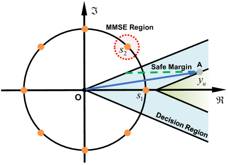
Figure 2: Illustration of the decision region, safe margin, and the MMSE region of a transmit symbol selected from the 8-PSK constellation.

From Theorem 2, the following interesting insights can be obtained:

Insight 3 (Design Guideline):

Since $\Psi(x)$ is a monotonically decreasing function, the communication BER performance can be enhanced by increasing the safe margin $\alpha_{u}$ or ensuring that $\alpha_{u}$ is greater than the lower SEP threshold. To facilitate understanding, we illustrate an 8-PSK constellation in Fig. 2. Suppose the received signal $y_{u}$ is at point A; the safe margin is then represented by the green dotted line. It is clear from Fig. 2 that if the safe margin of $y_{u}$ increases, $y_{u}$ moves farther away from the decision boundary, thereby decreasing the communication BER.

Insight 4 (Comparison to Conventional Metric):

In 1-bit communication scenarios, the MMSE is a widely used communication metric [34, 35, 22], aiming to ensure the received symbol $y_{u}$ is close to the desired symbol $s_{u}$ by mitigating multiuser interference (MUI). This restricts the received symbol $y_{u}$ within a circular region (red circular region in Fig. 2) around $s_{u}$, which limits design flexibility. In contrast, the Theorem 2 indicates that as long as the received signal remains within the safe margin, it can guarantee the communication BER performance, offering a new perspective to ensur communication BER performance.

III-B2 Communication Metric

Based on Insight 3, the communication performance of 1BitISAC can be guaranteed by maximizing $\alpha_{u}$. Alternatively, we can also constrain $\alpha_{u}$ to be greater than a threshold $\lambda_{u}$ to achieve communication BER performance that exceeds a desired bound. To flexibly control communication QoS performance, we set the threshold $\lambda_{u}$ as $\lambda_{u}=\sqrt{\Gamma_{u}\sigma_{\mathrm{C},u}^{2}}$ [38, 39, 23, 26], where $\Gamma_{u}$ is desired communication SNR.

To provide more insights on the meaning of (21) in communications, after some complex algebraic transformations, we equivalently re-express $\alpha_{u}$ in (21) as

$$\eqref{eq:27-n}\Leftrightarrow\alpha_{u}=\Re\left(\bar{{\bm{h}}}_{u}^{H}{\bm{x}}\right)-\cot\left(\frac{\pi}{\mathcal{M}}\right)\left|\Im\left(\bar{{\bm{h}}}_{u}^{H}{\bm{x}}\right)\right|.$$ (22)

From (22), we give the following remark:

Remark 2:

It is observed that (22) shares the same form as the constructive interference (CI)-based symbol level precoding (SLP) metric [38, 39, 23, 26]. Specifically, CI is defined as the interference that pushes the noise-free received signal away from the decision boundary. From (22), we note that the safe-margin mathematically quantifies the effectiveness of CI in pushing the noise-free received signal away from the decision boundary. This analysis establishes a relationship between communication BER performance, safe margin, and CI-based SLP, highlighting the essence of CI-based SLP.

Based on the previous analyses and guidelines, in the following two sections, we shall reformulate the QoS-constrained and QoD-constrained design problems, and present the proposed solutions, along with convergence analysis.

IV QoS-Constrained 1BitISAC Design

IV-A Problem Formulation

Based on the analysis and metrics discussed in Section III, the QoS-constrained 1BitISAC design problem in (9) can be recast d as follows

$$\mathop{\max}\limits_{{{\bm{x}}},{{\bm{u}}}}\quad \mu\frac{{{\bm{u}}}^{H}{{\bm{G}}}_{0}{{\bm{x}}}{{\bm{x}}}^{H}{{\bm{G}}}_{0}^{H}{{\bm{u}}}}{\sum_{q=1}^{Q}{\mathrm{CNR}_{\mathrm{R},q}{{\bm{u}}}^{H}{{\bm{G}}}_{q}{{\bm{x}}}{{\bm{x}}}^{H}{{\bm{G}}}_{q}^{H}{{\bm{u}}}}+\|{{\bm{u}}}\|_{F}^{2}}$$ (23a)

$${\text{s}}.{\text{t}}.\quad \min\{\Re(\kappa_{1}\bar{{\bm{h}}}_{u}^{H}{\bm{x}}),\Re(\kappa_{2}\bar{{\bm{h}}}_{u}^{H}{\bm{x}})\}\geq\lambda_{u},\forall u$$ (23b)

$${{\bm{x}}}\in\mathcal{X}_{\text{DAC}}^{\text{1-Bit}}=\left\{\frac{E}{{\sqrt{2{M_{\text{T}}}}}}({\pm 1\pm\jmath})\right\},$$ (23c)

where $\mu=2\mathrm{SNR}_{\mathrm{R}}/\pi$ is a constant.

Before detailing the solutions to problem (23), some transformations will be performed. It is clear that problem (23) involves two variables, ${\bm{x}}$ and ${\bm{u}}$. Additionally, we observe that the receive filter ${\bm{u}}$ is only present in the objective of problem (23). Therefore, updating the receive filter ${\bm{u}}$ leads to the following unconstrained problem

$$\mathop{\max}\limits_{{{\bm{u}}}}\quad\mu\frac{{{\bm{u}}}^{H}{{\bm{G}}}_{0}{{\bm{x}}}{{\bm{x}}}^{H}{{\bm{G}}}_{0}^{H}{{\bm{u}}}}{\sum_{q=1}^{Q}{\mathrm{CNR}_{\mathrm{R},q}{{\bm{u}}}^{H}{{\bm{G}}}_{q}{{\bm{x}}}{{\bm{x}}}^{H}{{\bm{G}}}_{q}^{H}{{\bm{u}}}}+\|{{\bm{u}}}\|_{F}^{2}},$$ (24)

which is a typical Rayleigh quotient problem with closed-form solutions as

$${{\bm{u}}}=\frac{{{\Big{[}{\sum\limits_{q=1}^{Q}{\mathrm{CNR}_{\mathrm{R},q}{{{\bm{G}}}_{q}}{{\bm{x}}}{{\bm{x}}}^{H}{{\bm{G}}}_{q}^{H}}+{{\bm{I}}}}\Big{]}^{-1}}{{{\bm{G}}}_{0}}{{\bm{x}}}}}{{{{{\bm{x}}}^{H}}{{\bm{G}}}_{0}^{H}{\Big{[}{\sum\limits_{q=1}^{Q}{\mathrm{CNR}_{\mathrm{R},q}{{{\bm{G}}}_{q}}{{\bm{x}}}{{\bm{x}}}^{H}{{\bm{G}}}_{q}^{H}}+{{\bm{I}}}}\Big{]}^{-1}}{{{\bm{G}}}_{0}}{{\bm{x}}}}}.$$ (25)

By substituting ${\bm{u}}$ from (25) into the objective function of (23), the problem (23) can be further formulated as follows

$$\mathop{\max}\limits_{{{\bm{x}}}}\;\; \text{QSCNR}({{\bm{x}}})$$ (26a)

$${\text{s}}.{\text{t}}.\;\; \min\{\Re(\kappa_{1}\bar{{\bm{h}}}_{u}^{H}{\bm{x}}),\Re(\kappa_{2}\bar{{\bm{h}}}_{u}^{H}{\bm{x}})\}\geq\lambda_{u},\forall u$$ (26b)

$${{\bm{x}}}\in\mathcal{X}_{\text{DAC}}^{\text{1-Bit}}=\left\{\frac{E}{{\sqrt{2{N_{\text{T}}}}}}({\pm 1\pm\jmath})\right\},$$ (26c)

where $\text{QSCNR}({{\bm{x}}})$ is given by

$$\text{QSCNR}({{\bm{x}}})$$ (27)

$$=\mu{{{{\bm{x}}}^{H}}{{\bm{G}}}_{0}^{H}{\Big{[}{\sum\limits_{q=1}^{Q}{\mathrm{CNR}_{\mathrm{R},q}{{{\bm{G}}}_{q}}{{\bm{x}}}{{\bm{x}}}^{H}{{\bm{G}}}_{q}^{H}}+{{\bm{I}}}}\Big{]}^{-1}}{{{\bm{G}}}_{0}}{{\bm{x}}}}.$$

Now, we end up with an optimization problem involving a single variable, i.e., ${\bm{x}}$. The remaining challenges in solving (26) lie in the complicated objective function and the discrete values of ${\bm{x}}$. In the next subsection, we will address these challenges and present the solution to problem (26).

IV-B Proposed Solution to Problem (26)

IV-B1 MM for Objective Function (26a)

The objective function (26a) is a complex fractional function with inverse operation. We apply MM approaches to simplify (26a) into more tractable linear function. Specifically, we first present the following proposition to address the inverse operation in (26).

Proposition 1:

Let ${{\bm{M}}}$ be a Hermitian matrix, a minorizer of ${\bm{s}}^{H}{\bm{M}}^{-1}{\bm{s}}$ is given by

$${\bm{s}}^{H}{\bm{M}}^{-1}{\bm{s}}\geq 2\Re\{{\bm{s}}_{t}^{H}{\bm{M}}_{t}^{-1}{\bm{s}}\}-\text{Tr}\left\{{\bm{M}}_{t}^{-1}{\bm{s}}_{t}{\bm{s}}_{t}^{H}{\bm{M}}_{t}^{-1}{\bm{M}}\right\},$$ (28)

where $({\bm{s}}_{t},{\bm{M}}_{t})$ represent the point at $t$-th iteration.

Proof:

See [40, Section III]. ∎

By submitting ${\bm{M}}={\sum_{q=1}^{Q}{\mathrm{CNR}_{\mathrm{R},q}{{{\bm{G}}}_{q}}{{\bm{x}}}{{\bm{x}}}^{H}{{\bm{G}}}_{q}^{H}}+{{\bm{I}}}}$ and ${\bm{s}}={\bm{G}}_{0}{\bm{x}}$ into Proposition 1, we have

$$\text{QSCNR}({{\bm{x}}})\geq-\mu\text{Tr}\left\{{\bm{M}}_{t}^{-1}{\bm{G}}_{0}{\bm{x}}_{t}{\bm{x}}_{t}^{H}{\bm{G}}_{0}^{H}{\bm{M}}_{t}^{-1}{\bm{M}}\right\}$$

$$\quad+2\mu\Re\left\{{\bm{x}}_{t}^{H}{\bm{G}}_{0}^{H}{\bm{M}}_{t}^{-1}{\bm{G}}_{0}{\bm{x}}\right\}+\text{const}_{1}$$ (29a)

$$=-\mu{\bm{x}}^{H}\widetilde{{\bm{M}}}_{t}{\bm{x}}+2\mu\Re\left\{{\bm{x}}_{t}^{H}{\bm{G}}_{0}^{H}{\bm{M}}_{t}^{-1}{\bm{G}}_{0}{\bm{x}}\right\}+\text{const}_{1}$$ (29b)

$$=\widehat{\text{QSCNR}}({{\bm{x}}}|{{\bm{x}}}_{t}),$$ (29c)

where $\text{const}_{1}=-\mu\text{Tr}\{{\bm{M}}_{t}^{-1}{\bm{G}}_{0}{\bm{x}}_{t}{\bm{x}}_{t}^{H}{\bm{G}}_{0}^{H}{\bm{M}}_{t}^{-1}\}$ and $\widetilde{{\bm{M}}}_{t}=\sum_{q=1}^{Q}\mathrm{CNR}_{\mathrm{R},q}{{\bm{G}}}_{q}^{H}{\bm{M}}_{t}^{-1}{\bm{G}}_{0}{\bm{x}}_{t}{\bm{x}}_{t}^{H}{\bm{G}}_{0}^{H}{\bm{M}}_{t}^{-1}{{\bm{G}}}_{q}$.

So far, we have transformed the complicated objective function in (26a) into a quadratic function $\widehat{\text{QSCNR}}({{\bm{x}}}|{{\bm{x}}}_{t})$ by using MM approach. To further simplify $\widehat{\text{QSCNR}}({{\bm{x}}}|{{\bm{x}}}_{t})$, we can apply the MM approach again and have the following proposition.

Proposition 2:

Let ${{\bm{J}}}$ be a Hermitian matrix, a majorizer of ${\bm{x}}^{H}{\bm{J}}{\bm{x}}$ can be given by

$${\bm{x}}^{H}\!{\bm{J}}{\bm{x}}\!\leq\!\varpi_{\text{m}}\!\left\|{\bm{x}}\right\|_{F}^{2}\!+\!2\Re\!\left\{{\bm{x}}_{t}({\bm{J}}\!-\!\varpi_{\text{m}}{\bm{I}}){\bm{x}}\right\}\!-\!{\bm{x}}_{t}({\bm{J}}\!-\!\varpi_{\text{m}}{\bm{I}}){\bm{x}}_{t},$$ (30)

where $\varpi_{\text{m}}$ represents the maximum eigenvalue of ${\bm{J}}$, and ${\bm{I}}$ denotes the identity matrix.

Proof:

See [40, Section III-C, Example 13]. ∎

Therefore, by defining ${\bm{J}}=\widetilde{{\bm{M}}}_{t}$ and recognizing $\|{\bm{x}}\|_{F}^{2}=E$, we have

$$\text{QSCNR}({{\bm{x}}})\geq\widehat{\text{QSCNR}}({{\bm{x}}}|{{\bm{x}}}_{t})$$

$$\geq-2\mu\Re\left\{{\bm{x}}_{t}^{H}(\widetilde{{\bm{M}}}_{t}-\ell_{\text{max}}{\bm{I}}){\bm{x}}\right\}+2\mu\Re\left\{{\bm{x}}_{t}^{H}{\bm{G}}_{0}^{H}{\bm{M}}_{t}^{-1}{\bm{G}}_{0}{\bm{x}}\right\}$$

$$\quad-\mu\ell_{\text{max}}E+\mu{\bm{x}}_{t}(\widetilde{{\bm{M}}}_{t}-\ell_{\text{max}}{\bm{I}}){\bm{x}}_{t}+\text{const}_{1}$$ (31a)

$$=\Re\left\{{\bm{w}}_{t}^{H}{\bm{x}}\right\}+\text{const}_{2}=\overline{\text{QSCNR}}({{\bm{x}}}|{{\bm{x}}}_{t}).$$ (31b)

where $\ell_{\text{max}}$ is maximum eigenvalue of $\widetilde{{\bm{M}}}_{t}$, ${\bm{w}}_{t}$ is defined as ${\bm{w}}_{t}=2\mu{\bm{G}}_{0}{\bm{M}}_{t}^{-1}{\bm{G}}_{0}^{H}{\bm{x}}_{t}-2\mu(\widetilde{{\bm{M}}}_{t}-\ell_{\text{max}}{\bm{I}}){\bm{x}}_{t}$ and $\text{const}_{2}=\text{const}_{1}-\mu\ell_{\text{max}}E+\mu{\bm{x}}_{t}(\widetilde{{\bm{M}}}_{t}-\ell_{\text{max}}{\bm{I}}){\bm{x}}_{t}$.

By the transformation from (29) to (31), we have simplified $\text{QSCNR}({{\bm{x}}})$ to a linear function $\overline{\text{QSCNR}}({{\bm{x}}}|{{\bm{x}}}_{t})$, significantly reducing the design complexity.

IV-B2 Rearrangement for QoS Constraint (26b)

We propose to rearrange (26b) to facilitate the design. To this end, by noting $\min\{a,b\}\geq c\Rightarrow\{a>c,b>c\}$, we have

$$\eqref{eq:32b} \Leftrightarrow\min\{\Re(\kappa_{1}\bar{{\bm{h}}}_{u}^{H}{\bm{x}}),\Re(\kappa_{2}\bar{{\bm{h}}}_{u}^{H}{\bm{x}})\}\geq\lambda_{u},$$ (32)

$$\Leftrightarrow\left\{\Re\left\{\kappa_{1}\bar{{\bm{h}}}_{u}^{H}{\bm{x}}\right\}\geq\lambda_{u},\Re\left\{\kappa_{2}\bar{{\bm{h}}}_{u}^{H}{\bm{x}}\right\}\geq\lambda_{u}\right\},$$

$$\Leftrightarrow\Re\left\{{\bm{A}}_{u}{\bm{x}}\right\}\geq\lambda_{u}{\bm{1}}_{2}={\bm{\lambda}}_{u},$$

where ${\bm{1}}_{N}\in\mathbb{R}^{N}$ is a summing vector with all entries 1, ${\bm{A}}_{u}=[\kappa_{1},\kappa_{2}]^{T}\otimes\bar{{\bm{h}}}_{u}^{H}$, and ${\bm{\lambda}}_{u}=\lambda_{u}{\bm{1}}_{2}$.

IV-B3 Integer Linear Programming (ILP) for (26)

Based on the above reformulations, the original problem (26) can be transformed into

$$\mathop{\max}\limits_{{{\bm{x}}}}\quad \Re\left\{{\bm{w}}_{t}^{H}{\bm{x}}\right\}$$ (33a)

$${\text{s}}.{\text{t}}.\quad \Re\left\{{\bm{A}}{\bm{x}}\right\}\geq{\bm{\lambda}}$$ (33b)

$${{\bm{x}}}\in\mathcal{X}_{\text{DAC}}^{\text{1-Bit}}=\left\{\frac{E}{{\sqrt{2{N_{\text{T}}}}}}({\pm 1\pm\jmath})\right\}.$$ (33c)

where ${\bm{A}}=[{\bm{A}}_{1}^{T},\cdots,{\bm{A}}_{U}^{T}]^{T}$ and ${\bm{\lambda}}=[{\bm{\lambda}}_{1}^{T},\cdots,{\bm{\lambda}}_{U}^{T}]^{T}$. Now, the challenge in solving (33) lies in the discrete constraint (33c). To address this, we reformulate problem (33) into its real form as follows

$$\mathop{\max}\limits_{\widetilde{{{\bm{x}}}}}\quad \Re\left\{\widetilde{{\bm{w}}}_{t}^{T}\widetilde{{\bm{x}}}\right\}$$ (34a)

$${\text{s}}.{\text{t}}.\quad\;\; \widetilde{{\bm{A}}}\widetilde{{\bm{x}}}\geq\widetilde{{\bm{\lambda}}}$$ (34b)

$$\widetilde{{{\bm{x}}}}\in\mathcal{X}_{\text{DAC},\Re}^{\text{1-Bit}}=\left\{-\frac{E}{{\sqrt{2{N_{\text{T}}}}}},+\frac{E}{{\sqrt{2{N_{\text{T}}}}}}\right\}.$$ (34c)

where $\widetilde{{\bm{x}}}=[\Re\{{\bm{x}}^{T}\},\Im\{{\bm{x}}^{T}\}]^{T}$, $\widetilde{{\bm{w}}}=[\Re\{{\bm{w}}^{T}\},-\Im\{{\bm{w}}^{T}\}]^{T}$ and $\widetilde{{\bm{A}}}=\left[\begin{array}[]{ll}\Re\{{\bm{A}}\}&-\Im\{{\bm{A}}\}\\ \Im\{{\bm{A}}\}&\Re\{{\bm{A}}\}\end{array}\right]$. Problem (34) is a standard ILP with binary constraint (34c), which can be optimally solved using many existing solvers, such as branch and bound (BnB), implicit enumeration methods, and others. Here, we adopt the BnB method to tackle (34). For details of the BnB method, interested readers are referred to [38, 41, 42].

Finally, we present the pseudo code of the proposed solution to QoS-constrained 1BitISAC design in Algorithm 1.

Input : System Parameter

Output : ${\bm{u}}$ and ${\bm{x}}$

1 Initialization: Set ${\bm{x}}_{0}$ and $t=0$;

2 while No Convengence do

3       $t=t+1$;

4       Update ${{\bm{x}}}_{t}$ by solving (34) ;

5      

6 end while

7${{\bm{x}}}={{\bm{x}}}_{t}$;

${{\bm{u}}}=\frac{{{{\left[{\sum_{q=1}^{Q}{\mathrm{CNR}_{\mathrm{R},q}{{{\bm{G}}}_{q}}{{\bm{x}}}{{\bm{x}}}^{H}{{\bm{G}}}_{q}^{H}}+{{\bm{I}}}}\right]}^{-1}}{{{\bm{G}}}_{0}}{{\bm{x}}}}}{{{{{\bm{x}}}^{H}}{{\bm{G}}}_{0}^{H}{{\left[{\sum_{q=1}^{Q}{\mathrm{CNR}_{\mathrm{R},q}{{{\bm{G}}}_{q}}{{\bm{x}}}{{\bm{x}}}^{H}{{\bm{G}}}_{q}^{H}}+{{\bm{I}}}}\right]}^{-1}}{{{\bm{G}}}_{0}}{{\bm{x}}}}}$ .

Algorithm 1 Proposed solution to QoS-constrained 1BitISAC design problem (23).

IV-C Convergence Analysis

The following theorem is essential to show the convergence of the proposed Algorithm 1.

Theorem 3:

Assume that the sequence of the objective values generated by Algorithm 1 is $\{\text{QSCNR}({\bm{x}}_{t})\}$, then sequence is non-decreasing and will converge to a local maximum.

Proof:

See Appendix C. ∎

V QoD-Constrained 1BitISAC Design

In this section, we extend the proposed method in Section IV to the QoD-constrained 1BitISAC design in (10).

V-A Problem Reformulation

Similarly, guided by the performance analysis in Section III, the QoD-constrained 1BitISAC design in (10) can be recast as

$$\mathop{\max}\limits_{{{\bm{x}}},{{\bm{u}}}} \;\min_{u}\{\Re(\kappa_{1}\bar{{\bm{h}}}_{u}^{H}{\bm{x}}),\Re(\kappa_{2}\bar{{\bm{h}}}_{u}^{H}{\bm{x}})\}$$ (35a)

$${\text{s}}.{\text{t}}.\; \frac{2}{\pi}\frac{\mathrm{SNR}_{\mathrm{R}}{{\bm{u}}}^{H}{{\bm{G}}}_{0}{{\bm{x}}}{{\bm{x}}}^{H}{{\bm{G}}}_{0}^{H}{{\bm{u}}}}{\sum_{q=1}^{Q}{\mathrm{CNR}_{\mathrm{R},q}{{\bm{u}}}^{H}{{\bm{G}}}_{q}{{\bm{x}}}{{\bm{x}}}^{H}{{\bm{G}}}_{q}^{H}{{\bm{u}}}}+\|{{\bm{u}}}\|_{F}^{2}}\geq\chi$$ (35b)

$${{\bm{x}}}\in\mathcal{X}_{\text{DAC}}^{\text{1-Bit}}=\left\{\frac{E}{{\sqrt{2{M_{\text{T}}}}}}({\pm 1\pm\jmath})\right\},$$ (35c)

where $\chi\geq 0$ represents the radar QSCNR threshold. For the desired $\ln\mathrm{Pr}_{\mathrm{FA}}$ and $\mathrm{Pr}_{\mathrm{D}}$, $\chi\geq 0$ can be determined by $\chi=\ln\mathrm{Pr}_{\mathrm{FA}}/\mathrm{Pr}_{\mathrm{D}}-1$.

V-B Proposed Solution to (35)

Similarly to problem (23), after introducing auxiliary variable $\lambda$, applying the MM to the constraint set (35b) and rearranging (35a), problem (35) can be transformed into a simpler form as follows

$$\mathop{\max}\limits_{{\bm{x}},\lambda}\quad \lambda$$ (36a)

$${\text{s}}.{\text{t}}.\quad \Re\left\{{\bm{A}}{\bm{x}}\right\}\geq\lambda{\bm{1}}_{2U}$$ (36b)

$$\overline{\text{QSCNR}}({{\bm{x}}}|{{\bm{x}}}_{t})=\Re\left\{{\bm{w}}_{t}^{H}{\bm{x}}\right\}+\text{const}_{2}\geq\chi$$ (36c)

$${{\bm{x}}}\in\mathcal{X}_{\text{DAC}}^{\text{1-Bit}}=\left\{\frac{E}{{\sqrt{2{N_{\text{T}}}}}}({\pm 1\pm\jmath})\right\},$$ (36d)

where ${\bm{w}}_{t}$, ${\bm{A}}$, and $\text{const}_{2}$ share the same formulas as those in Section IV. By converting problem (36) into its real-valued form, we have the following standard ILP problem

$$\mathop{\max}\limits_{\widetilde{{\bm{x}}},\lambda}\quad \lambda$$ (37a)

$${\text{s}}.{\text{t}}.\quad \widetilde{{\bm{A}}}\widetilde{{\bm{x}}}\geq\lambda{{\bm{1}}}_{2U}$$ (37b)

$$\Re\left\{\widetilde{{\bm{w}}}_{t}^{T}\widetilde{{\bm{x}}}\right\}+\text{const}_{2}\geq\chi$$ (37c)

$$\widetilde{{{\bm{x}}}}\in\left\{-\frac{E}{{\sqrt{2{N_{\text{T}}}}}},+\frac{E}{{\sqrt{2{N_{\text{T}}}}}}\right\},$$ (37d)

which can also be optimally solved by BnB solver. Since the algorithm workflow and convergence analysis to problem (35) follows the same procedure as described in Section IV, the details are omitted for simplicity.

VI Numerical Examples

In this section, numerical examples are provided to evaluate the performance of the 1BitISAC.

VI-A System Setup

Before presenting the simulation results, the parameter settings, benchmark approaches, and evaluation metrics are introduced in this subsection.

VI-A1 Parameter Settings

Unless otherwise specified, in all simulations, the parameters are set as follows. The DFRC BS equipped with ${M_{\rm T}}=128$ transmit and ${M_{\rm R}}=128$ receive antennas transmits data streams to serve $U=4$ downlink users. We set the available transmit power as $E=1\text{W}$. We assume the same noise power $\sigma_{\mathrm{C},u}^{2},\forall u$ at users, i.e., $\sigma_{\mathrm{C}}^{2}=\sigma_{\mathrm{C},u}^{2}$. Consider that DFRC BS detects a target located in angle $\theta_{0}=10^{\circ}$, in presence of $Q=2$ clutter sources, which are located in angles $\theta_{1}=-50^{\circ}$ and $\theta_{2}=30^{\circ}$, respectively. The radar SNR and CNR is set as $\mathrm{SNR}_{\mathrm{R}}=15\text{dB}$ and $\mathrm{CNR}_{\mathrm{R},q}=30\text{dB},\forall q$, respectively.

VI-A2 Benchmark Approaches

For comparison purposes, we include ISAC systems with different configurations as below:

i): ISAC with $\infty$-Bit DAC, $\infty$-Bit ADC. This configuration is known as the conventional fully-digital architecture. This benchmark can be obtained by modifying the proposed solutions in the following ways: replace the QSCNR with SCNR in [37] and replace ${\bm{x}}\in\mathcal{X}_{\text{DAC}}^{\text{1-Bit}}$ with $\|{\bm{x}}\|_{F}^{2}=E$.

ii): ISAC with $\infty$-Bit DAC, 1-Bit ADC. This benchmark can be obtained by replacing ${\bm{x}}\in\mathcal{X}_{\text{DAC}}^{\text{1-Bit}}$ with $\|{\bm{x}}\|_{F}^{2}=E$ in the proposed solutions.

iii): ISAC with 1-Bit DAC, $\infty$-Bit ADC. This benchmark can be obtained by replacing the QSCNR with SCNR in [37] in the proposed solutions.

For consistency in notation, we refer to the proposed 1BitISAC system as the ISAC with 1-Bit DAC and 1-Bit ADC.

VI-A3 Evaluation Metrics

To thoroughly evaluate the performance of ISAC systems with different configurations, we define three evaluation metrics as follows:

i): Radar Energy Efficiency. To compare the energy efficiency (EE) for ISAC with different configurations, we define the radar EE as below

$$\text{REE}={\text{SCNR}}/{E_{\text{tol}}},$$ (38)

where $E_{\text{tol}}=(N_{\mathrm{T}}+N_{\mathrm{R}})(E_{\text{RF}}+E_{\text{LNA}})+2E_{\text{BB}}+2N_{\mathrm{T}}E_{\text{ADC}}+2N_{\mathrm{R}}E_{\text{DAC}}$ is the total power consumption. $E_{\text{RF}}$, $E_{\text{LNA}}$, and $E_{\text{BB}}$ represent the power consumption of the RF chain, low-noise amplifier, and baseband signal processing, respectively. These are set at 40 mW, 20 mW, and 200 mW. The $E_{\text{ADC}}$ are modeled as $E_{\text{ADC}}=\text{FOM}_{w}\times f_{s}\times 2^{B}$, where $f_{s}=1$GHz is the Nyquist sampling rate, $B$ is the number of ADC bits, $\text{FOM}_{w}=500$ fJ/conversion-step is Walden’s figure-of-merit for evaluating ADC’s power efficiency with resolution and speed [43, 44]. We assume that the power consumption for the DAC $E_{\text{DAC}}$ follows the same model as that for the ADC $E_{\text{ADC}}$ [43, 44]. We use 10-bit ADC/DAC ($B=10$) to approximate the power consumption of $\infty$-bit ADC/DAC.

ii): Monte Carlo QSCNR. To validate the theoretical performance analysis (TA) presented in Section III-A, we employ Monte Carlo (MC) simulations to calculate the practical QSCNR. Specifically, the theoretical QSCNR (TA) is calculated using (17), while the practical QSCNR (MC) is determined through $N_{\mathrm{R}}^{\text{MC}}=1e^{6}$ MC simulations.

iii): Monte Carlo BER. Similarly, to validate the performance TA in Section III-B, the practical BER is calculated by MC with $N_{\mathrm{C}}^{\text{MC}}=1e^{6}$ being the number of MC simulations.

VI-B QoS-Constrained 1BitISAC Design

In this subsection, we examine the performance of the 1BitISAC design proposed in Section IV, where the communication QoS requirement is constrained to facilitate comparison and validate radar performance. We assume the 8-PSK modulated symbols are used in the simulations, i.e., $\mathcal{M}=8$. We set the $\text{SNR}_{\mathrm{C},u}={{P}}/{\sigma_{\mathrm{C},u}^{2}}=\text{5dB},\forall u$. The communication QoS threshold $\lambda_{u}$ are set the same, i.e., $\lambda_{u}=\sqrt{\sigma_{c}^{2}\Gamma},\forall u$ [38], with $\Gamma$ being the communication QoS threshold.

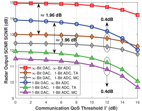
Figure 3: Radar output SCNR versus communication QoS threshold $\Gamma$.

Example 1. Impact of Communication QoS Threshold: In Fig. 3, we examine the radar output SCNR performance with different communication thresholds $\Gamma$. From Fig. 3, we can obtain the following observations: 1): A trade-off exists between radar output SCNR and communication QoS requirements. Specifically, as the communication QoS requirement $\Gamma$ increases, the radar output SCNR decreases for all methods. This occurs because the radar and communication systems compete for design resources. 2): With a small communication QoS threshold $\Gamma$, quantizing with 1-bit DACs results in a 1dB SCNR loss compared to the ideal $\infty$-Bit DACs. The performance gap between 1-bit and $\infty$-Bit DACs becomes more pronounced as the communication threshold $\Gamma$ increases. 3): Across all communication QoS thresholds $\Gamma$, the loss between ISAC systems with $\infty$-Bit ADCs and one-bit ADCs is about 1.96dB, which confirms Insight 1. Furthermore, the gap between the theoretical SCNR and the one obtained by MC simulations is only about 0.4dB.

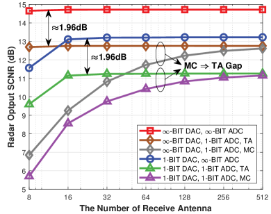
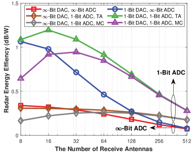
Figure 4: Radar performance with different number of receive antennas $N_{\mathrm{R}}$. (a) Radar output SCNR versus the number of receive antennas $N_{\mathrm{R}}$. (b) Radar EE versus the number of receive antennas $N_{\mathrm{R}}$.

Example 2. Impact of the Number of Receive Antennas $N_{\mathrm{R}}$: In Fig. 4, we present the radar output SCNR versus the number of receive antennas $N_{\mathrm{R}}$. From Fig. 4, we can obtain the following observations: 1): The gap between the TA of 1-bit ADCs and $\infty$-Bit ADCs remains consistently around 1.96dB. 2): The gap between the TA and MC for the 1-bit ADCs becomes increasingly negligible as the number of receive antennas $N_{\mathrm{R}}$ increases. To be more specific, when the number of receive antennas reaches $N_{\mathrm{R}}=128$, the gap between TA and MC is less than 0.4dB. Combining the above two observations, we can conclude that the performance analysis and Insight 2 presented in Section III are accurate.

In Fig. 4, we present the radar EE versus the number of receive antennas $N_{\mathrm{R}}$. It is evident that for ISAC with all configurations, increasing the number of receive antennas leads to a degradation in radar EE. Furthermore, the ISAC system with $\infty$-Bit ADCs and $\infty$-Bit DACs exhibits the worst radar EE performance, while the ISAC system with 1-bit ADCs and 1-bit DACs outperforms all other ISAC configurations. These results demonstrate that the ISAC system with 1-bit ADCs and 1-bit DACs is the most energy efficient strategy among the ISAC systems evaluated.

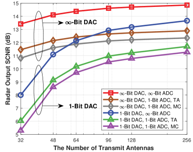
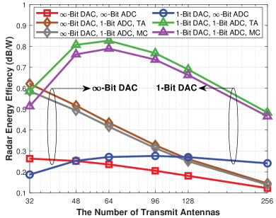
Figure 5: Radar performance with different number of transmit antennas $N_{\mathrm{T}}$. (a) Radar output SCNR versus the number of transmit antennas $N_{\mathrm{T}}$. (b) Radar EE versus the number of transmit antennas $N_{\mathrm{T}}$.

Example 3. Impact of the Number of Transmit Antennas $N_{\mathrm{T}}$: In Fig. 5, we study the radar output SCNR versus the the number of transmit antennas $N_{\mathrm{T}}$. From Fig. 5, we can obtain the following observations: 1): For all ISAC systems, with the increase in the number of transmit antennas $N_{\mathrm{T}}$, the radar output SCNR firstly improves significantly, and tends to saturate. This result indicates that a moderately large number of $N_{\mathrm{T}}$ is sufficient to achieve satisfactory performance, while further increasing the number of $N_{\mathrm{T}}$ does not result in further performance improvements, and instead causing significant power consumption and hardware cost. 2): Compared with the $\infty$-Bit DACs, the performance for ISAC systems with 1-bit DACs improves more remarkably with the number of the $N_{\mathrm{T}}$. This is because the quantization by 1-bit DACs results in a discrete sequence $\mathcal{X}_{\text{DAC}}^{\text{1-Bit}}$, which has fewer degrees of freedom and is more sensitive to changes in the number of $N_{\mathrm{T}}$.

In Fig. 5, we present the radar EE versus the number of transmit antennas $N_{\mathrm{R}}$. Similar to the trends observed in Fig. 4, as the number of transmit antennas $N_{\mathrm{T}}$ increases, all ISAC systems show a decreasing trend in radar EE performance. Notably, the ISAC system with 1-bit ADC and 1-bit DAC outperforms those with other configurations, validating the effectiveness of adopting this architecture in massive MIMO scenarios. Additionally, the ISAC system with 1-bit ADC and 1-bit DAC reaches its peak performance at $N_{\mathrm{T}}=64$, demonstrating that a moderate number of transmit antennas can effectively balance performance and EE.

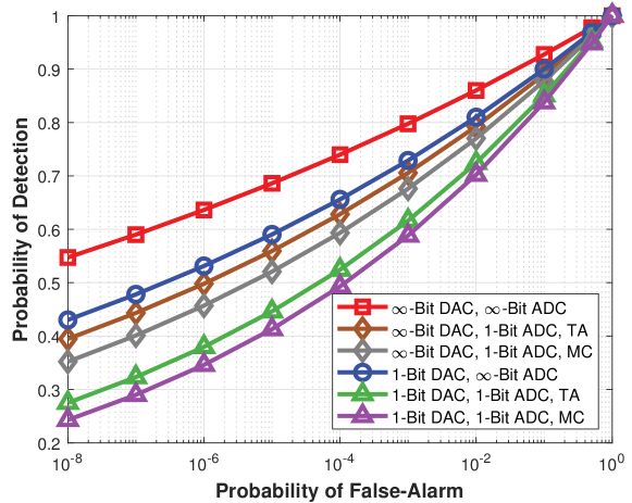
Figure 6: ROC of the ISAC detector with $\Gamma=12$dB.

Example 4. Radar Detection Performance: In Fig. 6, we show the radar receiver operating characteristic (ROC) of the ISAC detector proposed in Section III with communication QoS threshold $\Gamma=12$dB. We observe that the probability of detection $\mathrm{Pr}_{\mathrm{D}}$ for all ISAC systems increases with the probability of false-alarm $\mathrm{Pr}_{\mathrm{FA}}$. In addition, the probability of detection gap decreases with increasing probability of false-alarm. Moreover, by combining the data from Figs. 3 and 6, we can conclude that higher SCNR yields better detection performance. This observation validates the radar detection performance analysis presented in Section III-A.

VI-C QoD-Constrained 1BitISAC Design

In this subsection, we examine the performance of the 1BitISAC design proposed in Section V, where the radar SNCR requirement is constrained to facilitate comparison and validate communication performance. In the validation simulations, we use 8-PSK modulation with a radar SCNR threshold of $\chi=12$ dB and $N_{\mathrm{T}}=32$ transmit antennas.

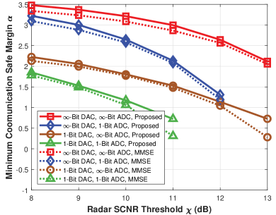
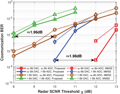
Figure 7: Communication performance evaluation with $\text{SNR}_{\mathrm{C}}=15$dB. (a) Minimum communication safe margin $\alpha$ (objective value in (35)) versus radar SCNR threshold $\chi$. (b) Communication BER versus radar SCNR threshold.

Example 5. Impact of Radar SCNR Threshold: In Fig. 7, we study the impact of radar SCNR threshold $\chi$ to communication performance. From Fig. 7, we observe that as the radar SCNR threshold increases, the minimum communication safe margin $\alpha$ decreases for all ISAC systems. Additionally, across all considered radar SCNR thresholds, the minimum communication safe margin $\alpha$ for the adopted proposed metric is consistently larger than that of the conventional MMSE-based design. This validates the effectiveness of the proposed safe margin metric in pushing the received signal within the safe margin. As expected, from Fig. 7, we observe that as the radar SCNR threshold increases, the communication BER also increases for all ISAC systems. Additionally, the ISAC systems employing safe margin technology are able to achieve lower BER performance compared to those using the MMSE-based design. Fig. 7 highlights the advantages and effectiveness of the proposed safe margin-based design in guaranteeing communication BER performance in ISAC.

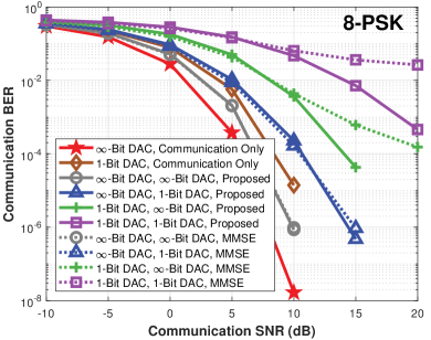
(a) 8-PSK

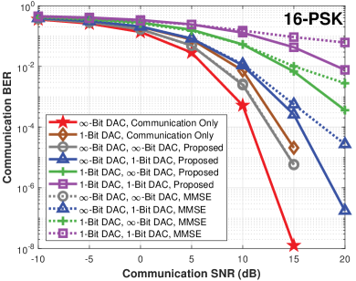
(b) 16-PSK

Figure 8: Communication BER versus the communication $\text{SNR}_{\mathrm{C}}$ with different modulation order $\mathcal{M}$.

Example 6. Impact of Modulation Order: In Fig. 8, we present the communication BER performance versus the communication $\text{SNR}_{\mathrm{C}}$ with different PSK modulation order. From Fig. 8, we obtain the following three observations: 1): For all PSK modulation orders and methods, as the communication $\text{SNR}_{\mathrm{C}}$ gradually increases, the communication BER performance improves. 2): When the communication $\text{SNR}_{\mathrm{C}}$ is 10dB or less, safe margin and MMSE-based ISAC systems can achieve nearly the same communication performance. However, when the communication $\text{SNR}_{\mathrm{C}}$ exceeds 10dB, the safe margin-based design in ISAC systems with a 1-bit architecture can achieve better performance than the MMSE-based design. 3): Increasing the PSK modulation order $\mathcal{M}$ leads to worse communication BER performance. This is because higher-order modulation results in smaller PSK decision regions, making the system more sensitive to noise and interference.

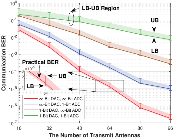
Figure 9: Communication BER versus the number of transmit antennas $N_{\mathrm{T}}$.

Example 8. Validation of SEP boundary: In Fig. 9, we show the communication BER versus the number of transmit antennas $N_{\mathrm{T}}$ with $\text{SNR}_{\text{C}}=5$dB. From Fig. 9, we observe the same trends as in Fig. 5, where increasing the number of transmit antennas $N_{\mathrm{T}}$ leads to more favorable communication BER performance. Additionally, for all ISAC systems, the practical BER consistently falls within the lower-bound (LB) and upper-bound (UB) region. These results validate Theorem 2 and verify that maximizing the safe margin is an effective strategy to guarantee communication BER performance.

VI-D Convergence Performance

In this subsection, we examine the performance of convergence performance of the proposed algorithms. Parameter settings are the same as those used in the above two subsections.

TABLE I: CPU Time (Seconds) Versus the Number of Receive Antennas

ISAC Configurations		The Number of Receive Antennas $N_{\mathrm{R}}$
DAC	ADC	16	32	64	128	256	512
$\infty$-Bit	$\infty$-Bit	1.08	1.43	1.55	1.88	1.97	2.26
	1-Bit	1.38	1.61	1.67	1.89	1.98	2.27
1-Bit	$\infty$-Bit	5.17	5.19	4.86	6.21	6.73	6.89
	1-Bit	4.91	4.96	5.00	6.55	6.75	7.10

TABLE II: CPU Time (Seconds) Versus the Number of Transmit Antennas

ISAC Configurations		The Number of Receive Antennas $N_{\mathrm{T}}$
DAC	ADC	32	48	64	96	128	256
$\infty$-Bit	$\infty$-Bit	0.64	0.64	0.64	0.64	0.65	0.67
	1-Bit	0.65	0.64	0.64	0.65	0.65	0.67
1-Bit	$\infty$-Bit	0.56	1.04	2.86	4.61	5.48	6.92
	1-Bit	0.55	1.02	2.55	4.75	5.64	7.02

Example 9. Comparison of Computational Efficiency: Tables I and II present the CPU time (in seconds) versus the number of receive antennas $N_{\mathrm{R}}$ and transmit antennas $N_{\mathrm{T}}$ for QoS-constrained design, respectively. As expected, we observe that as the number of receive antennas $N_{\mathrm{R}}$ and transmit antennas $N_{\mathrm{T}}$ increase, the CPU time required also increases. Compared with ISAC systems with $\infty$-Bit DACs, ISAC systems with 1-bit DACs take more time to converge. This increased time is due to the binary optimization required by the 1-bit ADC, which is computationally intensive. Additionally, we find that ISAC systems with either 1-bit or $\infty$-Bit DACs does not impact the convergence time significantly. Furthermore, the proposed method can converge within 10 seconds, which verifies the computational efficiency of the proposed approach.

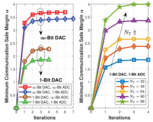
Figure 10: Convergence property of all ISAC systems with $\chi=8$dB.

Example 10. Comparison of Convergence Efficiency: In Fig. 10, we present the convergence behavior of the proposed solutions for the QoD-constrained design. From the left side of Fig. 10, it is evident that for all ISAC systems, the objective function becomes stationary after several iterations, which verifies the convergence efficiency of the proposed algorithm. Additionally, we observe similar trends where $\infty$-Bit DACs provide more degrees of freedom, allowing convergence to larger values, while 1-bit DACs converge to lower values. From the right side of Fig. 10, as expected, increasing the number of transmit antennas $N_{\mathrm{T}}$ leads to convergence to higher values, which aligns with the results observed in Fig. 9. Furthermore, for ISAC systems with different numbers of transmit antennas $N_{\mathrm{T}}$, the proposed algorithm can always converge within 10 iterations, demonstrating again the efficiency of the proposed algorithm.

VII Conclusion

In this paper, we investigated the joint transceiver design for an 1BitISAC system with massive MIMO. Two 1BitISAC designs, i.e., QoS-constrained 1BitISAC design and QoD-constrained 1BitISAC design, were considered. To guide the design of the 1BitISAC system, we first analyzed the radar detection performance following 1-bit ADC quantization. Subsequently, the communication BER performance was also analyzed, providing a new design perspective for measuring the communication performance in the 1BitISAC sysrem. Based on insights from these analyses, the design problems were reformulated and solved. Numerous simulation results were provided, revealing the following insights:

• After 1-bit ADC quantization, the proposed 1BitISAC system suffers from roughly a 1.98 dB performance loss, aligning with the performance analysis. These results highlight the feasibility of adopting 1-bit ADCs in massive MIMO ISAC systems, with an predictable and acceptable level of performance loss.

• Compared with the conventional communication MMSE, the derived safe margin-based method achieves better communication BER performance. These results verifies the BER analysis and supports the new design perspective in 1BitISAC.

• Compared with other ISAC configurations, the proposed 1BitISAC achieves the best EE performance in massive MIMO ISAC systems, albeit at the cost of slight performance sacrifices. These results indicate that the proposed 1BitISAC successfully balances the trade-off between EE and ISAC performance.

Appendix A Proof of Theorem 1

Defining $\widetilde{\bm{r}}^{\Re}=\Re\{\widetilde{\bm{r}}\}$ and $\widetilde{\bm{r}}^{\Im}=\Im\{\widetilde{\bm{r}}\}$, $\text{Pr}(\widetilde{\bm{r}}^{\Re}|\mathcal{H}_{i})$ and $\text{Pr}(\widetilde{\bm{r}}^{\Im}|\mathcal{H}_{i})$ can be given by [45]

$$\text{Pr}(\widetilde{\bm{r}}^{\Re}|\mathcal{H}_{i}) =\prod\limits_{n=1}^{2{M_{\text{R}}}}{{\left[{{\text{Pr}}\left({[\widetilde{\bm{r}}^{\Re}]_{n}=1|{\mathcal{H}_{i}}}\right)}\right]}^{\frac{{[\widetilde{\bm{r}}^{\Re}]_{n}+1}}{2}}}$$

$$\qquad\quad\times{{\left[{{\text{1}}-{\text{Pr}}\left({[\widetilde{\bm{r}}^{\Re}]_{n}=1|{\mathcal{H}_{i}}}\right)}\right]}^{\frac{{1-[\widetilde{\bm{r}}^{\Re}]_{n}}}{2}}},$$ (39a)

$$\text{Pr}(\widetilde{\bm{r}}^{\Im}|\mathcal{H}_{i}) =\prod\limits_{n=1}^{2{M_{\text{R}}}}{{\left[{{\text{Pr}}\left({[\widetilde{\bm{r}}^{\Im}]_{n}=1|{\mathcal{H}_{i}}}\right)}\right]}^{\frac{{[\widetilde{\bm{r}}^{\Im}]_{n}+1}}{2}}}$$

$$\qquad\quad\times{{\left[{{\text{1}}-{\text{Pr}}\left({[\widetilde{\bm{r}}^{\Im}]_{n}=1|{\mathcal{H}_{i}}}\right)}\right]}^{\frac{{1-[\widetilde{\bm{r}}^{\Im}]_{n}}}{2}}},$$ (39b)

where ${{\text{Pr}}\left({[\widetilde{\bm{r}}^{\Re}]_{n}=1|{\mathcal{H}_{i}}}\right)}$ and ${{\text{Pr}}\left({[\widetilde{\bm{r}}^{\Im}]_{n}=1|{\mathcal{H}_{i}}}\right)}$ represent the probabilities of $[\widetilde{\bm{r}}^{\Re}]_{n}=1$ and $[\widetilde{\bm{r}}^{\Im}]_{n}=1$ under $\mathcal{H}_{i}$, respectively. Then, according to definitions of ${{\text{Pr}}\left({[\widetilde{\bm{r}}^{\Re}]_{n}=1|{\mathcal{H}_{i}}}\right)}$ and ${{\text{Pr}}\left({[\widetilde{\bm{r}}^{\Im}]_{n}=1|{\mathcal{H}_{i}}}\right)}$, we have

$${{\text{Pr}}\left({[\widetilde{\bm{r}}^{\Re}]_{n}=1|{\mathcal{H}_{i}}}\right)}=1-\Phi\left(\frac{-[{\bm{r}}_{i}^{\Re}]_{n}}{\sqrt{\sigma_{\mathrm{R}}^{2}/2}}\right),$$ (40a)

$${{\text{Pr}}\left({[\widetilde{\bm{r}}^{\Im}]_{n}=1|{\mathcal{H}_{i}}}\right)}=1-\Phi\left(\frac{-[{\bm{r}}_{i}^{\Im}]_{n}}{\sqrt{\sigma_{\mathrm{R}}^{2}/2}}\right),$$ (40b)

where ${\bm{r}}_{i}^{\Re}=\Re\{{\bm{r}}_{i}\}$, ${\bm{r}}_{i}^{\Im}=\Im\{{\bm{r}}_{i}\}$ and $\Phi(x)=\frac{1}{\pi}\int_{-\infty}^{x}{e^{-t^{2}}}\text{d}t$.

According to (39), we can obtain the expectation $\mathbb{E}\{[\widetilde{\bm{r}}]_{n}|\mathcal{H}_{i}\}$ of $[\widetilde{\bm{r}}]_{n}$ under $\mathcal{H}_{i}$, which is

$$\mathbb{E} \{[\widetilde{\bm{r}}]_{n}|\mathcal{H}_{i}\}=\mathbb{E}\{[\widetilde{\bm{r}}^{\Re}]_{n}|\mathcal{H}_{i}\}+\jmath\mathbb{E}\{[\widetilde{\bm{r}}^{\Im}]_{n}|\mathcal{H}_{i}\}$$ (41)

$$=1-\Phi\left(\frac{-[{\bm{r}}_{i}^{\Re}]_{n}}{\sqrt{\sigma_{\mathrm{R}}^{2}/2}}\right)+\jmath\left(1-\Phi\left(\frac{-[{\bm{r}}_{i}^{\Im}]_{n}}{\sqrt{\sigma_{\mathrm{R}}^{2}/2}}\right)\right)$$

$$=\text{erf}\left(\frac{[{\bm{r}}_{i}^{\Re}]_{n}}{\sqrt{\sigma_{\mathrm{R}}^{2}}}\right)+\jmath\text{erf}\left(\frac{[{\bm{r}}_{i}^{\Im}]_{n}}{\sqrt{\sigma_{\mathrm{R}}^{2}}}\right).$$

The function $\text{erf}(\cdot)$ in (41) is complicated, which is not friendly for further derivation. To facilitate the formulation, recall the low SNR/CNR property in property 1, we observe that $\frac{[\widetilde{\bm{r}}_{i}^{\Re}]_{n}}{\sqrt{\sigma_{\mathrm{R}}^{2}}}\to 0$ and $\frac{[\widetilde{\bm{r}}_{i}^{\Im}]_{n}}{\sqrt{\sigma_{\mathrm{R}}^{2}}}\to 0$. Since $\text{erf}(\cdot)$ is a continuous function with $\text{erf}(x)=\text{erf}^{\prime}(0)x+o(x)=\frac{2}{\sqrt{\pi}}x+o(x)$, we can derive the asymptotic expectation $\mathbb{E}\{[\widetilde{\bm{r}}]_{n}\}$ as

$$\mathbb{E} \{[\widetilde{\bm{r}}]_{n}|\mathcal{H}_{i}\}=\text{erf}\left(\frac{[{\bm{r}}_{i}^{\Re}]_{n}}{\sqrt{\sigma_{\mathrm{R}}^{2}}}\right)+\jmath\text{erf}\left(\frac{[{\bm{r}}_{i}^{\Im}]_{n}}{\sqrt{\sigma_{\mathrm{R}}^{2}}}\right)$$ (42)

$$=\frac{2}{\sqrt{\pi}}\left(\frac{[{\bm{r}}_{i}^{\Re}]_{n}}{\sqrt{\sigma_{\mathrm{R}}^{2}}}+\jmath\frac{[{\bm{r}}_{i}^{\Im}]_{n}}{\sqrt{\sigma_{\mathrm{R}}^{2}}}\right)+o\left(\frac{[{\bm{r}}_{i}^{\Re}]_{n}}{\sqrt{\sigma_{\mathrm{R}}^{2}}}\right)+\jmath o\left(\frac{[{\bm{r}}_{i}^{\Im}]_{n}}{\sqrt{\sigma_{\mathrm{R}}^{2}}}\right)$$

$$=\frac{2}{\sqrt{\pi}}\frac{[{\bm{r}}_{i}]_{n}}{\sqrt{\sigma_{\mathrm{R}}^{2}}}+o\left(\frac{[{\bm{r}}_{i}]_{n}}{\sqrt{\sigma_{\mathrm{R}}^{2}}}\right).$$

Based on (42), the variance $\mathbb{D}\{[\widetilde{\bm{r}}_{i}]_{n}|\mathcal{H}_{i}\}$ can be given by

$$\mathbb{D}\{[\widetilde{\bm{r}}]_{n}|\mathcal{H}_{i}\} =\mathbb{E}\{\left|[\widetilde{\bm{r}}]_{n}\right|^{2}|\mathcal{H}_{i}\}-\left|\mathbb{E}\{[\widetilde{\bm{r}}]_{n}|\mathcal{H}_{i}\}\right|^{2}$$ (43)

$$=2-\left|\mathbb{E}\{[\widetilde{\bm{r}}]_{n}|\mathcal{H}_{i}\}\right|^{2}\mathop{\approx}\limits^{(a)}2,$$

where $(a)$ is based on

$$\lim_{\left|\hbar\right|\to 0}\frac{\left|\mathbb{E}\{[\widetilde{\bm{r}}]_{n}|\mathcal{H}_{i}\}\right|^{2}}{\left|\hbar\right|}=\frac{\frac{4}{\pi}\left|\hbar\right|^{2}+\frac{4\Re\{\hbar o(\hbar)\}}{\sqrt{\pi}}+\left|o(\hbar)\right|^{2}}{\left|\hbar\right|}=0.$$ (44)

with $\hbar={[{\bm{r}}_{i}]_{n}}/{\sqrt{\sigma_{\mathrm{R}}^{2}}}$.

Based on the analysis of the mean and variance of $\widetilde{\bm{r}}$, we can obtain:

$$\mathbb{E}\{\widetilde{{\bm{r}}}|\mathcal{H}_{i},{\bm{\gamma}}_{i}\}=\frac{2}{\sqrt{\pi\sigma_{\mathrm{R}}^{2}}}{\bm{r}}_{i},\quad\mathbb{D}\{\widetilde{{\bm{r}}}|\mathcal{H}_{i},{\bm{\gamma}}_{i}\}=2{\bm{I}}_{N_{\mathrm{R}}}.$$ (45)

Then, based on the central limit theorem, as $N_{\mathrm{R}}\to\infty$ and recalling $z={\bm{u}}^{H}\widetilde{{\bm{r}}}={\bm{u}}^{H}\mathcal{Q}_{\text{ADC}}^{\text{1-Bit}}({\bm{r}}_{i}+{\bm{n}}_{\mathrm{R}})$, thus we have

$$\mathbb{E}\{z|\mathcal{H}_{i},{\bm{\gamma}}_{i}\}=\frac{2}{\sqrt{\pi\sigma_{\mathrm{R}}^{2}}}{\bm{u}}^{H}{\bm{r}}_{i},\;\;\;\mathbb{D}\{z|\mathcal{H}_{i},{\bm{\gamma}}_{i}\}=2\|{\bm{u}}\|_{F}^{2}.$$ (46)

According to (46), we have

$$\text{Pr}\left(z|\mathcal{H}_{i},{\bm{\gamma}}_{i}\right)=\frac{1}{2\pi\left\|{\bm{u}}\right\|_{F}^{2}}\exp\Bigg{(}-\frac{\big{|}z-\frac{2}{\sqrt{\pi\sigma_{\mathrm{R}}^{2}}}{\bm{u}}^{H}{\bm{r}}_{i}\big{|}^{2}}{2\left\|{\bm{u}}\right\|_{F}^{2}}\Bigg{)}.$$ (47)

The proof is completed.

Appendix B Proof of Theorem 2

Since the $\mathcal{M}$-PSK constellation possesses the symmetry property, the SEP analysis for every symbol is identical and yields the same results. Without loss of generality, we assume $s_{u}=e^{\jmath\frac{2\pi\times 0}{\mathcal{M}}}=1$. Therefore the SEP in (19) can be simplified as

$$\mathrm{SEP}_{u}\triangleq\mathrm{Pr}\left(\left|\Im\left(y_{u}\right)\right|\geq\tan\left(\frac{\pi}{\mathcal{M}}\right)\Re\left(y_{u}\right)\right).$$ (48)

The SEP in (48) can be upper bounded by

$$\mathrm{SEP}_{u}\triangleq \mathrm{Pr}\left(\left|\Im\left(y_{u}\right)\right|\geq\tan\left(\frac{\pi}{\mathcal{M}}\right)\Re\left(y_{u}\right)\right)$$ (49)

$$\leq \mathrm{Pr}\left(\Im\left(y_{u}\right)\geq\tan\left(\frac{\pi}{\mathcal{M}}\right)\Re\left(y_{u}\right)\right)$$

$$+\mathrm{Pr}\left(-\Im\left(y_{u}\right)\geq\tan\left(\frac{\pi}{\mathcal{M}}\right)\Re\left(y_{u}\right)\right).$$

The SEP in (48) can be lower bounded by

$$\mathrm{SEP}_{u}\triangleq \mathrm{Pr}\left(\left|\Im\left(y_{u}\right)\right|\geq\tan\left(\frac{\pi}{\mathcal{M}}\right)\Re\left(y_{u}\right)\right)$$ (50)

$$\geq \max\left\{\mathrm{Pr}\left(\Im\left(y_{u}\right)\geq\tan\left(\frac{\pi}{\mathcal{M}}\right)\Re\left(y_{u}\right)\right)\right.,$$

$$\qquad\;\;\left.\mathrm{Pr}\left(-\Im\left(y_{u}\right)\geq\tan\left(\frac{\pi}{\mathcal{M}}\right)\Re\left(y_{u}\right)\right)\right\}.$$

Then, we turn our eyes to analyses $\mathrm{Pr}(\Im(y_{u})\geq\tan(\frac{\pi}{\mathcal{M}})\Re(y_{u}))$, and $\mathrm{Pr}(-\Im(y_{u})\geq\tan(\frac{\pi}{\mathcal{M}})\Re(y_{u}))$. Recalling that $y_{u}={\bm{h}}_{u}^{H}{\bm{x}}+n_{\mathrm{C},u}$ in (7), we have

$$\mathrm{Pr}\left(\Im\left(y_{u}\right)\geq\tan\left(\frac{\pi}{\mathcal{M}}\right)\Re\left(y_{u}\right)\right)$$ (51)

$$=\mathrm{Pr}\left(\begin{array}[]{l}\Im\left({\bm{h}}_{u}^{H}{\bm{x}}\right)+\Im\left(n_{\mathrm{C},u}\right)\\ \qquad\quad\geq\tan\left(\frac{\pi}{\mathcal{M}}\right)\Re\left({\bm{h}}_{u}^{H}{\bm{x}}\right)+\tan\left(\frac{\pi}{\mathcal{M}}\right)\Re\left(n_{\mathrm{C},u}\right)\end{array}\right)$$

$$=\mathrm{Pr}\left(\cot\left(\frac{\pi}{\mathcal{M}}\right)\Im\left(n_{\mathrm{C},u}\right)-\Re\left(n_{\mathrm{C},u}\right)\geq\alpha_{u}^{1}\right).$$

where $\alpha_{u}^{1}=\Re\left({\bm{h}}_{u}^{H}{\bm{x}}\right)-\cot\left(\frac{\pi}{\mathcal{M}}\right)\Im\left({\bm{h}}_{u}^{H}{\bm{x}}\right)=\Re(\kappa_{1}{\bm{h}}_{u}^{H}{\bm{x}})$ with $\kappa_{1}=1-e^{-\jmath\frac{\pi}{2}}\cot(\frac{\pi}{\mathcal{M}})$. Since ${n_{\mathrm{C},u}}$ is the AWGN with ${n_{\mathrm{C},u}}\sim{\mathcal{CN}}\left({0,\sigma_{\mathrm{C},u}^{2}}\right)$, we have $\cot(\frac{\pi}{\mathcal{M}})\Im(n_{\mathrm{C},u})-\Re(n_{\mathrm{C},u})\sim{\mathcal{N}}\left({0,\frac{\sigma_{\mathrm{C},u}^{2}}{2\sin^{2}(\frac{\pi}{\mathcal{M}})}}\right)$. Thus, (51) can be further simplified as

$$\mathrm{Pr}\left(\Im\left(y_{u}\right)\geq\tan\left(\frac{\pi}{\mathcal{M}}\right)\Re\left(y_{u}\right)\right)=\Psi\left(\frac{\sqrt{2}\sin(\frac{\pi}{\mathcal{M}})\alpha_{u}^{1}}{\sigma_{\mathrm{C},u}}\right).$$ (52)

where $\Psi(x)=\frac{1}{\sqrt{2\pi}}\int_{x}^{\infty}{e^{-x^{2}/2}}\text{d}x$. Similarly, we have

$$\mathrm{Pr}\left(-\Im\left(y_{u}\right)\geq\tan\left(\frac{\pi}{\mathcal{M}}\right)\Re\left(y_{u}\right)\right)=\Psi\left(\frac{\sqrt{2}\sin(\frac{\pi}{\mathcal{M}})\alpha_{u}^{2}}{\sigma_{\mathrm{C},u}}\right).$$ (53)

where $\alpha_{u}^{2}=\Re\left({\bm{h}}_{u}^{H}{\bm{x}}\right)-\cot\left(\frac{\pi}{\mathcal{M}}\right)\Im\left({\bm{h}}_{u}^{H}{\bm{x}}\right)=\Re(\kappa_{2}{\bm{h}}_{u}^{H}{\bm{x}})$ with $\kappa_{2}=1+e^{-\jmath\frac{\pi}{2}}\cot(\frac{\pi}{\mathcal{M}})$.

Noting the monotonically decreasing property of $\Psi(x)$, defining $\alpha_{u}=\min\{\alpha_{u}^{1},\alpha_{u}^{2}\}$, and combining (48)-(51), we have

$$\Psi\left(\frac{\sqrt{2}\sin(\frac{\pi}{\mathcal{M}})\alpha_{u}}{\sigma_{\mathrm{C},u}}\right)\leq\mathrm{SEP}_{u}\leq 2\Psi\left(\frac{\sqrt{2}\sin(\frac{\pi}{\mathcal{M}})\alpha_{u}}{\sigma_{\mathrm{C},u}}\right).$$ (54)

For $s_{u}\neq 1$, following the same procedure above-mentioned yields the same SEP as in (54). Accordingly, $\alpha_{u}$ is defined as $\alpha_{u}=\min\{\alpha_{u}^{1},\alpha_{u}^{2}\}$ with $\alpha_{u}^{1}=\Re(\kappa_{1}\bar{{\bm{h}}}_{u}^{H}{\bm{x}})$, $\alpha_{u}^{2}=\Re(\kappa_{2}\bar{{\bm{h}}}_{u}^{H}{\bm{x}})$ and $\bar{{\bm{h}}}={\bm{h}}e^{\jmath\angle(s_{u})}$.

The proof is completed.

Appendix C Proof of Theorem 3

To prove the convergence of algorithm 1, it is sufficient to illustrate the following two issues.

1. Monotonicity: Based on the property of MM, it follows that

   QSCNR $$({{\bm{x}}}_{t})=\overline{\text{QSCNR}}({{\bm{x}}}_{t}|{{\bm{x}}}_{t})$$ (55)

   $$\leq\overline{\text{QSCNR}}({{\bm{x}}}_{t+1}|{{\bm{x}}}_{t})\leq{\text{QSCNR}}({{\bm{x}}}_{t+1}).$$

   As the index $t$ increases, $\overline{\text{QSCNR}}({{\bm{x}}}|{{\bm{x}}}_{t})$ is monotonically improving.

2. Boundedness: The boundedness of $\text{QSCNR}\left({\bm{x}}\right)$ can be showed by following inequalities

   $$\text{QSCNR}\left({\bm{x}}\right)\mathop{\leq}\limits^{(a)}\text{QSCNR}_{wo}\left({\bm{x}}\right)$$ (56)

   $$=\frac{2}{\pi}\mathrm{SNR}_{\mathrm{R}}{{{{\bm{x}}}^{H}}{{\bm{G}}}_{0}^{H}{{{\bm{G}}}_{0}}{{\bm{x}}}}=\frac{2}{\pi}\mathrm{SNR}_{\mathrm{R}}\|{\bm{g}}_{\mathrm{T}}^{T}(\theta_{0}){{\bm{x}}}\|_{F}^{2}$$

   $$\mathop{\leq}\limits^{(b)}\frac{2E}{\pi}\mathrm{SNR}_{\mathrm{R}}.$$

   where $(a)$ is because the $\text{QSCNR}\left({\bm{x}}\right)$ in the presence of clutter sources is always lower than in scenarios without clutter sources $\text{QSCNR}_{wo}\left({\bm{x}}\right)$. $(b)$ is because the optimal solution of $\max_{{\bm{x}}}\|{\bm{g}}_{\mathrm{T}}^{T}(\theta_{0}){{\bm{x}}}\|_{F}^{2}$ is ${\bm{x}}=\sqrt{E}{\bm{g}}_{T}^{*}(\theta_{0})$ with optimal value $E$. Since the transmit power $E$ is limited, the $\text{QSCNR}\left({\bm{x}}\right)$ is always bounded.

Based on above two properties, we can conclude the sequence $\{\text{QSCNR}({\bm{x}}_{t})\}$ is non-decreasing and converges to a local maximum. This completes the proof.

References

• [1] B. Wang, H. Li, and Z. Cheng, “Joint transceiver design for massive MIMO DFRC systems with one-bit DACs/ADCs,” in Proc. of 2023 IEEE Globecom Workshops (GC Wkshps).   IEEE, 2023, pp. 649–654.
• [2] F. Liu, L. Zheng, Y. Cui, C. Masouros, A. P. Petropulu, H. Griffiths, and Y. C. Eldar, “Seventy years of radar and communications: The road from separation to integration,” IEEE Signal Process. Mag., vol. 40, no. 5, pp. 106–121, 2023.
• [3] J. A. Zhang, F. Liu, C. Masouros, R. W. Heath, Z. Feng, L. Zheng, and A. Petropulu, “An overview of signal processing techniques for joint communication and radar sensing,” IEEE J. Sel. Topics Signal Process., vol. 15, no. 6, pp. 1295–1315, 2021.
• [4] F. Liu, C. Masouros, A. P. Petropulu, H. Griffiths, and L. Hanzo, “Joint radar and communication design: Applications, state-of-the-art, and the road ahead,” IEEE Trans. Commun., vol. 68, no. 6, pp. 3834–3862, 2020.
• [5] Y. Xiong, F. Liu, K. Wan, W. Yuan, Y. Cui, and G. Caire, “From torch to projector: Fundamental tradeoff of integrated sensing and communications,” IEEE BITS the Inform. Theory Mag., 2024.
• [6] C. Feng, W. S. A. Au, S. Valaee, and Z. Tan, “Received-signal-strength-based indoor positioning using compressive sensing,” IEEE Trans. Mobile Comput., vol. 11, no. 12, pp. 1983–1993, 2011.
• [7] D. Jiang and L. Delgrossi, “IEEE 802.11 p: Towards an international standard for wireless access in vehicular environments,” in Proc. of 2008 IEEE veh. technol. conf. (VTC Spring).   IEEE, 2008, pp. 2036–2040.
• [8] P. Kumari, J. Choi, N. González-Prelcic, and R. W. Heath, “IEEE 802.11 ad-based radar: An approach to joint vehicular communication-radar system,” IEEE Trans. Veh. Technol., vol. 67, no. 4, pp. 3012–3027, 2017.
• [9] Y. Li, F. Liu, Z. Du, W. Yuan, Q. Shi, and C. Masouros, “Frame structure and protocol design for sensing-assisted NR-V2X communications,” IEEE Trans. Mobile Comput., 2024.
• [10] M. Nowak, M. Wicks, Z. Zhang, and Z. Wu, “Co-designed radar-communication using linear frequency modulation waveform,” IEEE Aerosp. Electron. Syst. Mag., vol. 31, no. 10, pp. 28–35, 2016.
• [11] K. Wu, J. A. Zhang, X. Huang, and Y. J. Guo, “Frequency-hopping MIMO radar-based communications: An overview,” IEEE Aerosp. Electron. Syst. Mag., vol. 37, no. 4, pp. 42–54, 2021.
• [12] A. Ahmed, Y. D. Zhang, and Y. Gu, “Dual-function radar-communications using QAM-based sidelobe modulation,” Digital Signal Process., vol. 82, pp. 166–174, 2018.
• [13] K. Meng, C. Masouros, G. Chen, and F. Liu, “Network-level integrated sensing and communication: Interference management and BS coordination using stochastic geometry,” arXiv preprint arXiv:2311.09052, 2023.
• [14] Z. Liao, F. Liu, A. Li, and C. Masouros, “Faster-than-nyquist symbol-level precoding for wideband integrated sensing and communications,” IEEE Trans. Wireless Commun., 2024.
• [15] X. Liu, T. Huang, N. Shlezinger, Y. Liu, J. Zhou, and Y. C. Eldar, “Joint transmit beamforming for multiuser MIMO communications and MIMO radar,” IEEE Trans. Signal Process., vol. 68, pp. 3929–3944, 2020.
• [16] R. Liu, M. Li, Q. Liu, and A. L. Swindlehurst, “Dual-functional radar-communication waveform design: A symbol-level precoding approach,” IEEE J. Sel. Topics Signal Process., vol. 15, no. 6, pp. 1316–1331, 2021.
• [17] F. Liu, Y.-F. Liu, A. Li, C. Masouros, and Y. C. Eldar, “Cramér-rao bound optimization for joint radar-communication beamforming,” IEEE Trans. Signal Process., vol. 70, pp. 240–253, 2021.
• [18] B. Guo, J. Liang, B. Tang, L. Li, and H. C. So, “Bistatic MIMO DFRC system waveform design via symbol distance/direction discrimination,” IEEE Trans. Signal Process., vol. 71, pp. 3996–4010, 2023.
• [19] Z. Wei, J. Piao, X. Yuan, H. Wu, J. A. Zhang, Z. Feng, L. Wang, and P. Zhang, “Waveform design for MIMO-OFDM integrated sensing and communication system: An information theoretical approach,” IEEE Trans. Commun., vol. 72, no. 1, pp. 496–509, 2024.
• [20] X. Wang, B. Tang et al., “Relative entropy-based waveform optimization for rician target detection with dual-function radar communication systems,” IEEE Sensors J., vol. 23, no. 10, pp. 10 718–10 730, 2023.
• [21] J. Zhang, L. Dai, X. Li, Y. Liu, and L. Hanzo, “On low-resolution ADCs in practical 5G millimeter-wave massive MIMO systems,” IEEE Commun. Mag., vol. 56, no. 7, pp. 205–211, 2018.
• [22] O. Castañeda et al., “1-bit massive MU-MIMO precoding in VLSI,” IEEE J. on Emerging and Sel. Topics in Circuits and Syst., vol. 7, no. 4, pp. 508–522, 2017.
• [23] A. Li, C. Masouros, A. L. Swindlehurst, and W. Yu, “1-bit massive mimo transmission: Embracing interference with symbol-level precoding,” IEEE Commun. Mag., vol. 59, no. 5, pp. 121–127, 2021.
• [24] J. Mo, P. Schniter, and R. W. Heath, “Channel estimation in broadband millimeter wave mimo systems with few-bit ADCs,” IEEE Trans. Signal Process., vol. 66, no. 5, pp. 1141–1154, 2017.
• [25] M. Shao et al., “A framework for one-bit and constant-envelope precoding over multiuser massive MISO channels,” IEEE Trans. Signal Process., vol. 67, no. 20, pp. 5309–5324, 2019.
• [26] Z. Wu, B. Jiang, Y.-F. Liu, M. Shao, and Y.-H. Dai, “Efficient CI-based one-bit precoding for multiuser downlink massive MIMO systems with PSK modulation,” IEEE Trans. Wireless Commun., vol. 23, no. 5, pp. 4861–4875, 2024.
• [27] Z. Cheng, L. Wu, B. Wang, J. Xie, and H. Li, “Relative entropy-based constant-envelope beamforming for target detection in large-scale MIMO radar with low-resoultion ADCs,” IEEE Trans. Veh. Technol., vol. 72, no. 8, pp. 10 090–10 106, 2023.
• [28] F. Xi, Y. Xiang, S. Chen, and A. Nehorai, “Gridless parameter estimation for one-bit MIMO radar with time-varying thresholds,” IEEE Trans. Signal Process., vol. 68, pp. 1048–1063, 2020.
• [29] Y.-H. Xiao, D. Ramírez, P. J. Schreier et al., “One-bit target detection in collocated MIMO radar and performance degradation analysis,” IEEE Trans. Veh. Technol., vol. 71, no. 9, pp. 9363–9374, 2022.
• [30] M. Deng et al., “One-bit ADCs/DACs based MIMO radar: Performance analysis and joint design,” IEEE Trans. Signal Process., vol. 70, pp. 2609–2624, 2022.
• [31] X. Shang, R. Lin, and Y. Cheng, “Mixed-ADC based PMCW MIMO radar angle-Doppler imaging,” IEEE Trans. Signal Process., vol. 72, pp. 883–895, 2024.
• [32] X. Huang and B. Liao, “One-bit MUSIC,” IEEE Signal Process. Lett., vol. 26, no. 7, pp. 961–965, 2019.
• [33] S. Sedighi, B. S. Mysore R, M. Soltanalian, and B. Ottersten, “On the performance of one-bit DoA estimation via sparse linear arrays,” IEEE Trans. Signal Process., vol. 69, pp. 6165–6182, 2021.
• [34] Z. Cheng, S. Shi, Z. He, and B. Liao, “Transmit sequence design for dual-function radar-communication system with one-bit DACs,” IEEE Trans. Wireless Commun., vol. 20, no. 9, pp. 5846–5860, 2021.
• [35] X. Yu, Q. Yang, Z. Xiao, H. Chen, V. Havyarimana, and Z. Han, “A precoding approach for dual-functional radar-communication system with one-bit DACs,” IEEE J. Sel. Areas Commun., vol. 40, no. 6, pp. 1965–1977, 2022.
• [36] S. Jacobsson, G. Durisi, M. Coldrey, T. Goldstein, and C. Studer, “Quantized precoding for massive MU-MIMO,” IEEE Trans. Commun., vol. 65, no. 11, pp. 4670–4684, 2017.
• [37] G. Cui, H. Li, and M. Rangaswamy, “MIMO radar waveform design with constant modulus and similarity constraints,” IEEE Trans. Signal Process., vol. 62, no. 2, pp. 343–353, 2013.
• [38] A. Li, F. Liu, C. Masouros, Y. Li, and B. Vucetic, “Interference exploitation 1-bit massive MIMO precoding: A partial branch-and-bound solution with near-optimal performance,” IEEE Trans. Wireless Commun., vol. 19, no. 5, pp. 3474–3489, 2020.
• [39] A. Li, C. Masouros, F. Liu, and A. L. Swindlehurst, “Massive MIMO 1-bit DAC transmission: A low-complexity symbol scaling approach,” IEEE Trans. Wireless Commun., vol. 17, no. 11, pp. 7559–7575, 2018.
• [40] Y. Sun, P. Babu, and D. P. Palomar, “Majorization-minimization algorithms in signal processing, communications, and machine learning,” IEEE Trans. Signal Process., vol. 65, no. 3, pp. 794–816, 2016.
• [41] L. T. Landau and R. C. de Lamare, “Branch-and-bound precoding for multiuser MIMO systems with 1-bit quantization,” IEEE Wireless Commun. Lett., vol. 6, no. 6, pp. 770–773, 2017.
• [42] S. Boyd and J. Mattingley, “Branch and bound methods,” Notes for EE364b, Stanford University, vol. 2006, p. 07, 2007.
• [43] J. Mo et al., “Hybrid architectures with few-bit ADC receivers: Achievable rates and energy-rate tradeoffs,” IEEE Trans. Wireless Commun., vol. 16, no. 4, pp. 2274–2287, 2017.
• [44] R. H. Walden, “Analog-to-digital converter survey and analysis,” IEEE J. Sel. Areas Commun., vol. 17, no. 4, pp. 539–550, 1999.
• [45] C. Gianelli, L. Xu, J. Li, and P. Stoica, “One-bit compressive sampling with time-varying thresholds: Maximum likelihood and the Cramér-Rao bound,” in 2016 50th Asilomar Conference on Signals, Systems and Computers.   IEEE, 2016, pp. 399–403.